On $\lambda$-Cent-Dians and Generalized-Center for Network Design

Abstract

In this paper, we extend the notions of $\lambda$-cent-dian and generalized-center from Facility Location Theory to the more intricate domain of Network Design. Our focus is on the task of designing a sub-network within a given underlying network while adhering to a budget constraint. This sub-network is intended to efficiently serve a collection of origin/destination pairs of demand.

The $\lambda$-cent-dian problem studies the balance between efficiency and equity. We investigate the properties of the $\lambda$-cent-dian and generalized-center solution networks under the lens of equity, efficiency, and Pareto-optimality. We provide a mathematical formulation for $\lambda\geq 0$ and discuss the bilevel structure of this problem for $\lambda>1$. Furthermore, we describe a procedure to obtain a complete parametrization of the Pareto-optimality set based on solving two mixed integer linear formulations by introducing the concept of maximum $\lambda$-cent-dian. We evaluate the quality of the different solution concepts using some inequality measures. Finally, for $\lambda\in[0,1]$, we study the implementation of a Benders decomposition method to solve it at scale.

1 Introduction

Center and median problems in graphs and Euclidean spaces constituted the core of Location Science in the late 50s and 60s of the past century. Whereas median problems aim at maximizing the system’s efficiency, center ones try to maximize the effectiveness or equity. In the median problem, the objective is to find one or more facility locations (points) in a given space, such that the normalized sum of weighted distances from the demand points to their closest facility is minimized. In contrast, the center problem seeks to find one or more facility locations to minimize the largest distance from a demand point to the nearest facility.

On the other hand, the median problem is well-suited for situations where the primary objective is cost minimization or profit maximization within the system. On the other hand, the center problem is ideal for scenarios where the goal is to ensure that the farthest point is as close as possible to the facility, as in locating emergency facilities. However, when taken separately, these two objectives do not adequately address many real-world problems that require balancing efficiency and equity.

In Halpern (1976), the term $\lambda$-cent-dian was first introduced for location problems whose objective is to minimize a linear convex combination of center and median objectives, denoted by $F_{c}$ and $F_{m}$ respectively, i.e. the $\lambda$-cent-dian objective is $H_{\lambda}=\lambda F_{c}+(1-\lambda)F_{m}$. Subsequently, in Halpern (1978), the author proved that the $\lambda$-cent-dian of a graph lies on a path connecting the center and the median, and provided a procedure to find the $\lambda$-cent-dians for all possible combinations given by the different values of $\lambda$. An $O(|N||E|\log(|N||V|))$ time algorithm to find all the $\lambda$-cent-dian points is proposed by Hansen et al. (1991). Moreover, they also introduced the concept of generalized-center as the minimizer of the difference function between the center and the median. In fact, when $\lambda\rightarrow\infty$, the ratio $\frac{H_{\lambda}}{\lambda}$ tends to the generalized-center. The generalized-center is an objective that favors the equity between O/D pairs. However, it could lead to inefficient solutions as noted by Ogryczak (1997). An axiomatic approach to the $\lambda$-cent-dian criterion was given in Carrizosa (1994).

The $\lambda$-cent-dian objective has also been considered in extensive facility location problems. A facility is called extensive if it is too large regarding its environment to be represented by isolated points. Examples of extensive facilities are paths, cycles, or trees on graphs and straight lines, circles, or hyperplanes in Euclidean spaces (see Mesa & Boffey (1996), Puerto et al. (2009)).

The importance of the $\lambda$-cent-dian criterion allows weight, in some way, two contradicting criteria. Thus, the decision-maker chooses the weight to allocate to the center criterion and to the median criterion. To the best of our knowledge, we are the first to investigate and formalize the $\lambda$-cent-dian network design problem. In this context, our focus diverges from traditional facility location problems by identifying an optimal sub-network instead of single-point facilities and considering the demand given by origin-destination pairs (O/D pairs).

Network Design problems have been applied to several fields, especially in telecommunications and transportation systems (Crainic et al., 2021). In some cases, the demand is not represented by individual points but rather by pairs of points (e.g., O/D pairs representing telephone calls), which produce flows that the network must manage. In transportation, the applications are diverse: air transportation, postal delivery systems, service networks, trucking, and transit systems. Often, there is only one network that handles the flows between origins and destinations. However, in some instances, more than one network is already in operation. In these situations, there is competition among the existing systems to capture demand. For instance, in mobile telephony, there is stiff competition among various providers. In urban and metropolitan mobility, a range of transportation modes, including private cars, bicycles, buses, and metros, compete for commuters’ preferences.

Most Network Design problems primarily revolve around objective functions centered on either cost or profit. Given the inherent cost dependency on distance, these objective functions effectively serve as surrogates for the classical median problems, characterized by the summation of (weighted) distances to the facility. Furthermore, certain scenarios require additional considerations, where the proximity of origins and destinations plays a key role. For instance, in densely populated metropolitan areas, the daily commute of individuals to their workplaces necessitates minimal travel time, reflecting their reluctance to endure extended daily journeys between their residences and workplaces. This concern over commuting time can be viewed as a proxy for distance. Another example is electricity distribution generated by (solar, hydro, or wind) mini-power facilities in rural areas. In these cases, the electricity is provided at low voltage, and power losses increase with the distance (see Gokbayrak (2022)). Thus, in these contexts, the center objective must be considered, combined with the median one.

In this article, we exploit the structure of the problem when $\lambda\in[0,1]$ by exploring a Benders Decomposition approach. This scheme has been extensively studied for Network Design problems (see Magnanti et al. (1986); Fortz & Poss (2009); Marín & Jaramillo (2009); Botton et al. (2013)). We also extend the strong cuts introduced by Conforti & Wolsey (2019) to this setting. These cuts have shown competitive results in many applications in Facility Location and Network Design Problems (see Cordeau et al. (2019); Bucarey et al. (2022)).

The contributions of this work are the following:

• We extend the solution concepts from the Facility Location Theory of the $\lambda$-cent-dian and generalized-center to the more intricate area of Network Design. In this setting, we study the $\lambda$-cent-dian concept by considering the demand as a set of origin/destination pairs to be connected through a solution network. Furthermore, this solution network must satisfy a budget constraint. The $\lambda$-cent-dian concept examines the balance between efficiency and equity. Notably, the generalized-center aligns with the specific case of the $\lambda$-cent-dian concept when $\lambda\rightarrow\infty$, emphasizing the variance between the measures of efficiency and equity. We delve into the properties of the $\lambda$-cent-dian and generalized-center solution networks, exploring equity, efficiency, and Pareto-optimality concerning the bicriteria center/median problem. Similar to findings in Facility Location, we ascertain that the Pareto-optimality solution set in the Network Design context is not always fully derived from minimizing the $\lambda$-cent-dian function for $\lambda\in[0,1]$. Examples illustrating these concepts are provided throughout the article for clarity.

• We provide a mathematical formulation for the $\lambda$-cent-dian problem with $\lambda\geq 0$. Furthermore, we address the bilevel structure when $\lambda>1$, and we adjust the formulation for this case.

• We outline a method to give a full parametrization of the Pareto-optimality set based on solving two linear formulations. Then, we evaluate and discuss the quality of the different solution concepts considered using some inequality measures. This evaluation incorporates the generalized-center concept, which has been under-explored in existing literature.

• Finally, we test a Benders decomposition approach to solve the problem for the case $\lambda\in[0,1]$. We tackle the problem using a Benders decomposition implementation and the ideas exposed in Conforti & Wolsey (2019).

The structure of the paper is as follows: In Section 2, we extend different concepts involving the median and center functions from Location Science to the more complex area of Network Design and analyze and compare the different solutions. In Section 3, we present a mathematical formulation for $\lambda\geq 0$. Besides, we discuss the bilevel structure when $\lambda>1$, and we adjust the formulation for this case. Then, we describe a procedure to give a complete parametrization of the Pareto-optimality set based on solving two linear formulations. Then, in Section 4 we investigate the quality of the solution concepts developed in this work. We develop a Benders decomposition approach to solve the problem for the case $\lambda\in[0,1]$ along with efficient tools for finding facet-defining cuts provided in Conforti & Wolsey (2019), shown in Section 5. Finally, our conclusions are presented in Section 6.

2 Problems definition

2.1 Setting description

In this paper, we address a network design problem using an underlying undirected graph to be $\mathcal{N}=(N,E)$, with associated costs for each node $i\in N$ and each link $e\in E$, denoted by $b_{i}\geq 0$ and $c_{e}\geq 0$, respectively. For every link $e=\{i,j\}\in E$, we define two arcs: $a=(i,j)$ and $\hat{a}=(j,i)$. We denote the set of resulting arcs as $A$. The length of each arc $a\in A$ is denoted by $d_{a}\geq 0$. We employ the notation $i\in e$ if node $i$ is a terminal node of $e$. Note that length can be substituted by time to traverse, generalized cost, or any other parameter assigned to each arc. We denote the set of edges incident to node $i$ by $\delta(i)\subseteq E$. Analogously, $\delta^{+}(i),\delta^{-}(i)\subseteq A$ denote the sets of arcs going out and in of node $i$.

We assume that the mobility patterns are known and represented by a set $W\subset N\times N$ of origin/destination pairs (called O/D pairs), and a matrix collecting the expected demand between each O/D pair in a given period of time. Note that couples with equal origin and destination are not included in $W$. Specifically, for any given pair $w=(w^{s},w^{t})\in W$ where $w^{s}\neq w^{t}$, the demand traveling from the origin node $w^{s}\in N$ to the destination node $w^{t}\in N$ is known and denoted by $g^{w}>0$. The aggregate demand is represented by $G=\sum\limits_{w\in W}g^{w}$.

We also consider a private utility, $u^{w}>0$, modeling that there already exists a (unique) mode, referred to as the private mode, for meeting the demand. This mode competes with the potential network to be built on an all-or-nothing basis. In other words, an O/D pair $(w^{s},w^{t})$ will utilize the new network only if it offers a path between $w^{s}$ and $w^{t}$ whose length or utility is equal to or shorter than the associated private utility $u^{w}$. If these conditions are met, we say the O/D pair is covered or served by the constructed network. Additionally, for each $w\in W$, the subgraph $\mathcal{N}^{w}=(N^{w},E^{w})$ comprises all nodes and edges that belong to a path in $\mathcal{N}$ with a length less than or equal to $u^{w}$. The corresponding arc set is represented by $A^{w}$.

We are interested in subgraphs, denoted as $\mathcal{S}=(N_{\mathcal{S}},E_{\mathcal{S}})$, of $\mathcal{N}$ that can be constructed respecting a budget constraint. We represent this budget as a fraction $\alpha$ of the total cost of building the potential graph $\mathcal{N}$, noted by $C_{total}$. Therefore, a subgraph $\mathcal{S}$ is feasible if the condition

$$\sum_{i\in N_{\mathcal{S}}}b_{i}+\sum_{e\in E_{\mathcal{S}}}c_{e}\leq\alpha\left(\sum_{i\in N}b_{i}+\sum_{e\in E}c_{e}\right)=\alpha\,C_{total}$$ (2.1)

is met. For a fixed value of $\alpha\in[0,1]$, we denote by $\mathbfcal{N}^{\alpha}$ the set of all subgraphs of $\mathcal{N}$ satisfying (2.1).

For a given subgraph $\mathcal{S}$ and an O/D pair $w\in W$, the term $d_{\mathcal{S}}(w)$ represents the length of the shortest path from $w^{s}$ to $w^{t}$ within the subgraph $\mathcal{S}$. If it is not possible to connect a pair $w\in W$ within $\mathcal{S}$, we assume that $d_{\mathcal{S}}(w)=+\infty$. Taking this into account and given that each pair has an associated utility, each demand will travel from its origin to the destination on a path of length $\ell_{\mathcal{S}}(w)=\min\{d_{\mathcal{S}}(w),u^{w}\}$.

2.2 Solution concepts

We now introduce extensions of two solution concepts derived from location science, which are central to this work: the median and the center. For a given $\alpha\in(0,1)$, the (weighted) median is defined as a subgraph $\mathcal{S}_{m}$ in $\mathbfcal{N}^{\alpha}$ that minimizes the objective function

$$F_{m}(\mathcal{S})=\frac{1}{G}\sum_{w\in W}g^{w}\ell_{\mathcal{S}}(w).$$ (2.2)

Given two subnetworks $\mathcal{S}_{1},\mathcal{S}_{2}\subseteq\mathcal{N}$, it is said that $\mathcal{S}_{1}$ is more efficient that $\mathcal{S}_{2}$ iff $F_{m}(\mathcal{S}_{1})<F_{m}(\mathcal{S}_{2})$.

A subgraph $\mathcal{S}_{c}$ is called a center if it is a minimizer of the following objective function

$$F_{c}(S)=\max_{w\in W}\ell_{\mathcal{S}}(w).$$ (2.3)

Related to the notion of center, it can be considered the weighted-center solution. The weighted-center solution is defined as the subgraph $\mathcal{S}_{c}^{G}$ in $\mathcal{N}^{\alpha}$ that minimizes the objective function

$$F_{c}^{G}(\mathcal{S})=\frac{\max\limits_{w\in W}\left\{g^{w}\ell_{\mathcal{S}}(w)\right\}}{g^{w_{0}}},\quad w_{0}=\operatorname*{arg\,max}_{w\in W}\left\{g^{w}\ell_{\mathcal{S}}(w)\right\}.$$

Given that the center minimizes the maximum travel time, it could lead to inefficient solutions. This inefficiency is produced by not considering feasible subgraphs in which travel time decreases for some users maintaining the center objective function value. We depict this situation in Example 1.

Example 1

Consider the following network with a budget $\alpha\,C_{total}=90$. Figure 1 represents the underlying network where the couple labeling the edges represents building cost and length, respectively. Table 1 shows O/D pairs, private utility and demand of this example.

Origin	Destination	$u^{w}$	$g^{w}$
1	6	92	200
2	5	92	50
4	1	92	50

Table 1: Data in Example 1. We consider $\alpha\,C_{total}=90$.

Figure 1: Network in Example 1.

We observe that, with the given bound on the total cost, it is impossible to cover the three O/D pairs simultaneously. Hence, the objective value for the center is $F_{c}(\mathcal{S}_{0})=92$. Note that the empty subgraph, $\mathcal{S}_{0}=\emptyset$, has a center value $F_{c}(\mathcal{S}_{0})=92$, and it is thus an optimal solution for the center problem. In other words, not constructing anything can be optimal for the center problem. Furthermore, this solution also yields a median value $F_{m}(\mathcal{S}_{0})=92$. Now let us consider the following two subgraphs:

• $\mathcal{S}_{1}$ composed by node set $N_{1}=\{1,2,4,6\}$ and edge set $E_{1}=\{(1,2),(2,4),(4,6)\}$ such that O/D pairs $(1,6)$ and $(4,1)$ are served; and

• $\mathcal{S}_{2}$ with $N_{2}=\{1,2,4,5\}$ and $E_{2}=\{(1,2),(2,4),(4,5)\}$ such that O/D pairs $(2,5)$ and $(4,1)$ are served.

The solutions above have an objective function value for the center $F_{c}(\mathcal{S}_{1})=F_{c}(\mathcal{S}_{2})=92$, but the median objective changes. Indeed, these values are $F_{m}(\mathcal{S}_{1})\approxeq 85.33$ and $F_{m}(\mathcal{S}_{2})\approxeq 81.33$ respectively.

Example 2

Using the aforementioned notation, we examine a network as outlined in Table 2 and illustrated in Figure 4. In this example, the solution that optimizes the median does not serve the most distant pair or those with low demand. By contrast, when minimizing the center objective, a significantly larger value for the median objective emerges.

The optimal median and center subgraphs are illustrated in Figure 2 and 3, respectively. The computed values for the median and center objectives are as follows:

$$F_{m}(\mathcal{S}_{m})=\frac{1}{120}(5\cdot 92+65\cdot 20+50\cdot 45)=\frac{4010}{120}\approxeq 38.19,\quad F_{c}(\mathcal{S}_{m})=92,$$

$$F_{m}(\mathcal{S}_{c})=\frac{1}{120}(5\cdot 80+65\cdot 40+50\cdot 50)=\frac{5500}{120}\approxeq 52.38,\quad F_{c}(\mathcal{S}_{c})=80.$$

For the respective networks, it is noteworthy that even when considering the weighted-center, the loss in efficiency may still persist in specific scenarios. For instance, in this particular case, the optimal weighted-center remains $\mathcal{S}_{c}$ with a value of $F_{c}^{G}(\mathcal{S}_{c})=40$.

Figure 2: Median network in Example 2.

Figure 3: Center network in Example 2.

Origin	Destination	$u^{w}$	$g^{w}$
1	6	92	5
2	3	40	65
4	1	50	50

Table 2: Data in Example 2. We consider $\alpha\,C_{total}=90$.

Figure 4: Network in Example 2.

Examples 1 and 2 show the necessity of having a refined conceptual framework to consider solutions that are not dominated and capture the trade-off between both solution concepts. While the median generally prioritizes users located at the network’s center, often to the detriment of those in distant regions, the center distinctly favors those in remote areas without necessarily considering the efficiency of the design. Recognizing this need for balanced solutions, researchers in the field of location science have, since the 1970s, explored the $\lambda$-cent-dian concept (refer to Halpern (1976)). This concept represents a convex combination of both the center and median objectives. In the realm of network design, for a given $\lambda\in[0,1]$, the $\lambda$-cent-dian is a subgraph that aims to minimize the following objective function:

$$H_{\lambda}(S)=\lambda F_{c}(\mathcal{S})+(1-\lambda)F_{m}(\mathcal{S})=\lambda\max_{w\in W}\ell_{\mathcal{S}}(w)+(1-\lambda)\frac{1}{G}\sum_{w\in W}g^{w}\ell_{\mathcal{S}}(w),$$ (2.4)

As it is mentioned in Ogryczak (1997), the problem of finding the $\lambda$-cent-dian can be seen as the weighted version of finding the solution to the bi-criteria problem of minimizing objectives (2.2) and (2.3).

Hansen et al. (1991) introduced the concept of the generalized-center for facility location. This concept was formulated to reduce discrepancies in accessibility among users as much as possible. In this work, the generalized-center corresponds to a subgraph, $\mathcal{S}_{gc}$, which minimizes the disparity between the center and median objectives, denoted as $F_{gc}(\mathcal{S})$. When one considers the difference between the function $F_{m}(\mathcal{S})$ and the function $F_{c}^{G}(\mathcal{S})$, instead of $F_{c}(\mathcal{S})$, the resultant solution network is named the weighted-generalized-center. The objective function for this is denoted by $F_{gc}^{G}(\mathcal{S})$.

As we have observed in Example 1, one generalized-center is the empty subgraph, which is an unreasonable solution from the point of view of the median value. Example 3 exemplifies a situation where the generalized-center worsens both the center and the median values. To avoid such solution networks, the optimal solution network is restricted to the set of solution networks so-called as Pareto-optimal concerning the distances (of the shortest paths). A subgraph $\mathcal{S}\in\mathbfcal{N}^{\alpha}$ is Pareto-optimal with respect to the distances (travel times) if there does not exist a subgraph $\mathcal{S}^{\prime}\in\mathbfcal{N}^{\alpha}$ such that $\ell_{\mathcal{S}^{\prime}}(w)\leq\ell_{\mathcal{S}}(w),$ for all $w\in W$ where at least one of these inequalities is strictly satisfied. We denote the set of subgraphs satisfying this definition of Pareto-optimality as $\mathbfcal{PO}^{\alpha}$. Thus, we redefine the generalized-center as the optimal solution to the problem

$$\min\{F_{c}(\mathcal{S})-F_{m}(\mathcal{S}):\mathcal{S}\in\mathbfcal{PO}^{\alpha}\}.$$ (2.5)

In the same way, the weighted-generalized-center is defined as the optimal solution to the problem

$$\min\{|F^{G}_{c}(\mathcal{S})-F_{m}(\mathcal{S})|:\mathcal{S}\in\mathbfcal{PO}^{\alpha}\}.$$ (2.6)

The following examples depict the discussion above.

Example 3

Let us consider the following example described in Table 3 and Figure 5.

The generalized-center $\mathcal{S}_{gc}$ is:

$F_{c}(\mathcal{S}_{gc})-F_{m}(\mathcal{S}_{gc})=92-\frac{1}{105}(50\cdot 92+5\cdot 70+50\cdot 92)\approxeq 92-90.95$.

Nevertheless, there exists a network, $\mathcal{S}_{1}$, more efficient in terms of the distances of the shortest paths than $\mathcal{S}_{gc}$:

$F_{c}(\mathcal{S}_{1})-F_{m}(\mathcal{S}_{1})=40-\frac{1}{105}(50\cdot 30+5\cdot 20+50\cdot 40)\approxeq 40-34.28$

In fact, $\mathcal{S}_{1}$ is simultaneously the center and the median. Even if we minimize $F_{gc}^{G}(\,\cdot\,)$, instead of $F_{gc}(\,\cdot\,)$, the optimal solution does not change, which is $\mathcal{S}_{gc}$. Network $\mathcal{S}_{1}$ is Pareto-optimal with respect to the distances, but $\mathcal{S}_{gc}$ is not. Even more, each of the O/D pairs has its shortest path shorter in $\mathcal{S}_{1}$ than in $\mathcal{S}_{gc}$. Locating $\mathcal{S}_{gc}$ can worsen the center and median values. This solution does not capture the trade-off between the center and the median values.

Origin	Destination	$u^{w}$	$g^{w}$
1	2	92	50
2	6	100	5
4	1	92	50

Table 3: Data in Example 3. We consider $\alpha\,C_{total}=90$.

Figure 5: Network in Example 3.

Even when the problem of the generalized-center is constrained to the set $\mathbfcal{PO}^{\alpha}$, there is potential for obtaining highly inefficient solution graphs as optimal solutions. This is illustrated in Example $4$. Specifically, when minimizing the difference $F_{c}(\,\cdot\,)-F_{m}(\,\cdot\,)$, if multiple solution networks have the same $F_{c}(\,\cdot\,)$ value, the network with the least favorable $F_{m}(\,\cdot\,)$ value will be chosen.

Example 4

We depict in Table 4 and Figure 6 a situation where the generalized-center in $\mathbfcal{PO}^{\alpha}$ leads to a very inefficient solution.

Origin	Destination	$u^{w}$	$g^{w}$
1	2	35	50
2	4	35	30
3	1	35	30
4	3	35	20

Table 4: Data in Example 4. We consider $\alpha\,C_{total}=50$.

Figure 6: Network in Example 4.

The set $\mathbfcal{PO}^{\alpha}$ consists of:

$$F_{c}(\mathcal{S}_{1})-F_{m}(\mathcal{S}_{1})=30-\frac{1}{130}(50\cdot 10+30\cdot 30+30\cdot 10+20\cdot 10)=30-\frac{1900}{130}\approxeq 15.38$$

$$F_{c}(\mathcal{S}_{2})-F_{m}(\mathcal{S}_{2})=30-\frac{1}{130}(50\cdot 30+30\cdot 10+30\cdot 10+20\cdot 10)=30-\frac{2300}{130}\approxeq 12.30$$

$$F_{c}(\mathcal{S}_{3})-F_{m}(\mathcal{S}_{3})=30-\frac{1}{130}(50\cdot 10+30\cdot 10+30\cdot 30+20\cdot 10)=30-\frac{1900}{130}\approxeq 15.38$$

$$F_{c}(\mathcal{S}_{4})-F_{m}(\mathcal{S}_{4})=30-\frac{1}{130}(50\cdot 10+30\cdot 10+30\cdot 10+20\cdot 30)=30-\frac{1430}{130}\approxeq 19$$

The four solution networks belong to $\mathbfcal{PO}^{\alpha}$, and each one is a center. While $\mathcal{S}_{2}$ is the generalized-center, $\mathcal{S}_{4}$ is the most efficient network. One might assume that the issues highlighted with the median and center values are resolved when considering the weighted function. However, this is not the case. It is easy to check that the generalized-weighted-center remains $\mathcal{S}_{2}$.

The last example shows the necessity to revisit the notion of Pareto-optimality. We perform this by extending the notion of Pareto-optimality to the bi-criteria setting: a subgraph $\mathcal{S}$ is Pareto-optimal if there no exists another subgraph $\mathcal{S^{\prime}}$ in $\mathbfcal{N}^{\alpha}$ for which

$$F_{m}(S^{\prime})\leq F_{m}(S)\quad\mbox{ and }\quad F_{c}(S^{\prime})\leq F_{c}(S),$$ (2.7)

with one of the inequalities being strict. We call denote the set of subgraphs satisfying this property $\mathbfcal{PO}^{\alpha}_{2}$. Hence, we define the restricted-generalized-center as an optimal solution to the problem

$$\min\{F_{c}(\mathcal{S})-F_{m}(\mathcal{S}):\mathcal{S}\in\mathbfcal{PO}^{\alpha}_{2}\}.$$ (2.8)

Remark 1.

In Example 4, $\mathbfcal{PO}^{\alpha}_{2}$ is composed only of $\mathcal{S}_{4}$, then it is the unique minimizer of (2.8). Furthermore, it is easy to check that always $\mathbfcal{PO}^{\alpha}_{2}\subseteq\mathbfcal{PO}^{\alpha}$.

Analogous to the restricted-generalized-center, we introduce the $\lambda$-restricted-cent-dian. It is defined as the optimal solution to the problem:

$$\min\{H_{\lambda}(\mathcal{S}):\mathcal{S}\in\mathbfcal{PO}^{\alpha}_{2}\}.$$ (2.9)

Remark 2.

For $\lambda\in(0,1)$, the corresponding $\lambda$-cent-dian always belongs to the set $\mathbfcal{PO}^{\alpha}_{2}$. This can be easily proved by Reductio ad absurdum. Thus, in this case, the $\lambda$-restricted-cent-dian is simply a $\lambda$-cent-dian.

The statement of Remark 2 is not necessarily true for $\lambda\geq 1$, specifically for the limiting case $\lambda\rightarrow\infty$. As shown in Example 4, the generalized-center does not necessarily belong to the set $\mathbfcal{PO}^{\alpha}_{2}$. Besides, we will show that for all $\lambda\geq 1$ the corresponding $\lambda$-restricted-cent-dian is always a center. Note that, given a bound $\alpha$, the center of a general network $\mathcal{N}$ may be non-unique and, in such cases, not all centers belong to $\mathbfcal{PO}^{\alpha}_{2}$. This issue is shown in Example $4$. We know that $\mathbfcal{PO}^{\alpha}=\{\mathcal{S}_{1},\mathcal{S}_{2},\mathcal{S}_{3},\mathcal{S}_{4}\}$, but $\mathcal{S}_{1},\mathcal{S}_{2},\mathcal{S}_{3}\notin\mathbfcal{PO}^{\alpha}_{2}$. To belong to $\mathbfcal{PO}^{\alpha}_{2}$, the center must be unique or it must be the center with the best value of $F_{m}(\,\cdot\,)$. Thus, the center belonging to $\mathbfcal{PO}^{\alpha}_{2}$ is an optimal solution of the following lexicographic problem

$$\mbox{lex}\min\{[F_{c}(\mathcal{S}),F_{m}(\mathcal{S})]:\,\,\mathcal{S}\in\mathbfcal{N}^{\alpha}\}.$$ (2.10)

The lexicographic minimization in (2.10) entails that we first minimize $F_{c}(\,\cdot\,)$ on the set $\mathbfcal{N}^{\alpha}$. Subsequently, we minimize $F_{m}(\,\cdot\,)$ on the optimal subnetworks set determined by $F_{c}(\,\cdot\,)$. This second minimization step is only necessary when the optimal solution of $F_{c}(\,\cdot\,)$ is not unique. We refer to the optimal solution of (2.10) as a lexicographic cent-dian. It is important to highlight that the lexicographic cent-dian is also a center, and in the case where the center is unique, this center is also the lexicographic cent-dian.

Proposition 1.

Consider $\lambda\geq 1.$ The restricted-generalized-center and the $\lambda-$ restricted-cent-dian are lexicographic cent-dian in $\mathcal{N}^{\alpha}$. Conversely, any lexicographic cent-dian is a restricted generalized center and a $\lambda-$ restricted-cent-dian.

Proof.

Let $\mathcal{S}$ be the lexicographic cent-dian. That is, $F_{c}(\mathcal{S})\leq F_{c}(\mathcal{S}^{\prime})$ for any $\mathcal{S}^{\prime}\in\mathbfcal{N}^{\alpha}$, or, if $\exists\,\mathcal{S}^{\prime}\in\mathbfcal{N}^{\alpha}$ such that $F_{c}(\mathcal{S})=F_{c}(\mathcal{S}^{\prime})$, then $F_{m}(\mathcal{S})\leq F_{m}(\mathcal{S}^{\prime})$. Firstly, observe that $\mathcal{S}\in\mathbfcal{PO}_{2}^{\alpha}$. To continue, we consider $\mathcal{S}^{\prime}\in\mathbfcal{N}^{\alpha}$ a solution network of $\mathbfcal{PO}_{2}^{\alpha}$. If $\mathcal{S}^{\prime}$ is not a lexicographic cent-dian, then $F_{c}(\mathcal{S})<F_{c}(\mathcal{S}^{\prime})$ or, if $F_{c}(\mathcal{S})=F_{c}(\mathcal{S}^{\prime})$ then $F_{m}(\mathcal{S})<F_{m}(\mathcal{S}^{\prime})$. This second situation is not possible since $\mathcal{S}^{\prime}\in\mathbfcal{PO}_{2}^{\alpha}$. Hence, being in $\mathbfcal{PO}_{2}^{\alpha}$, $\mathcal{S}^{\prime}$ has to satisfy inequalities

$$F_{c}(\mathcal{S})<F_{c}(\mathcal{S}^{\prime})\quad\text{ and }\quad F_{m}(\mathcal{S})>F_{m}(\mathcal{S}^{\prime}).$$

Thus, $F_{c}(\mathcal{S}^{\prime})-F_{m}(\mathcal{S}^{\prime})>F_{c}(\mathcal{S})-F_{m}(\mathcal{S})$, which means that the restricted-generalized-center is a lexicographic cent-dian. Aditionally, for $\lambda\geq 1$, this property holds:

$$H_{\lambda}(\mathcal{S}^{\prime})=F_{c}(\mathcal{S}^{\prime})+(\lambda-1)(F_{c}(\mathcal{S}^{\prime})-F_{m}(\mathcal{S}^{\prime}))>F_{c}(\mathcal{S})+(\lambda-1)(F_{c}(\mathcal{S})-F_{m}(\mathcal{S}))=H_{\lambda}(\mathcal{S}),$$

which proves that the corresponding $\lambda$-restricted-cent-dian is a lexicographic cent-dian.

To finish the proof, since all lexicographic cent-dians have the same center value and median value, they are all restricted-generalized-centers and $\lambda$-restricted-cent-dians with $\lambda>1$. ∎

Proposition 1 provides us with a very simple characteristic of the $\lambda$-restricted-cent-dian for $\lambda\geq 1$. From this, we conclude that the $\lambda$-restricted-cent-dians for $\lambda\geq 1$ are simply the centers with the best median value. On the other hand, it means that the solution concept of the restricted-generalized-center does not provide us with any compromise between the median and center values.

2.3 On the relationship of $\lambda$-cent-dians and Pareto optimal solutions

Pareto optimal solutions, denoted as $\mathbfcal{PO}^{\alpha}_{2}$, offer a set of sub-networks that efficiently strike a balance between spatial efficiency and equity. This is achieved by compromising between the median and center objectives. On the other hand, the concept of $\lambda-$cent-dian seeks to find this balance through a linear combination of both objectives. However, the sub-networks produced by the $\lambda-$cent-dian do not encompass all the sub-networks in $\mathbfcal{PO}^{\alpha}_{2}$.

Indeed, Example 5 illustrates the fact that networks containing cycles might have sub-networks that belong to $\mathbfcal{PO}^{\alpha}_{2}$ but differ from $\mathcal{S}_{c}$, $\mathcal{S}_{m}$ and any $\lambda$-cent-dian for $\lambda\in[0,1]$.

Example 5

Consider the following potential network with the fixed bound $\alpha\,C_{total}=70$:

Origin	Destination	$u^{w}$	$g^{w}$
1	2	70	90
3	4	55	20
5	6	92	5

Table 5: Data in Example 5. We consider $\alpha\,C_{total}=70$.

Figure 7: Network in Example 5.

The median $\mathcal{S}_{m}$ is

$F_{m}(\mathcal{S}_{m})=\frac{1}{115}(90\cdot 10+20\cdot 55+5\cdot 92)=\frac{2460}{115}\approxeq 21.39$

$F_{c}(\mathcal{S}_{m})=92$

The network has a unique center $\mathcal{S}_{c}$:

$F_{m}(\mathcal{S}_{c})=\frac{1}{115}(90\cdot 70+20\cdot 55+5\cdot 20)=\frac{7500}{115}\approxeq 65.21$

$F_{c}(\mathcal{S}_{c})=70$

There is another subnetwork belonging to $\mathbfcal{PO}^{\alpha}_{2}$. The following network $\mathcal{S}_{1}$ has a better value for the average of the shortest paths than $\mathcal{S}_{c}$ and its center value is lower than in $\mathcal{S}_{m}$.

$F_{m}(\mathcal{S}_{1})=\frac{1}{115}(90\cdot 60+20\cdot 35+5\cdot 80)=\frac{6500}{115}\approxeq 56.52$

$F_{c}(\mathcal{S}_{1})=80$

We can check that for any $0\leq\lambda\leq 1$, $H_{\lambda}(\mathcal{S}_{m})<H_{\lambda}(\mathcal{S}_{1})$ or $H_{\lambda}(\mathcal{S}_{c})<H_{\lambda}(\mathcal{S}_{1})$. That is, even though $\mathcal{S}_{1}\in\mathbfcal{PO}^{\alpha}_{2}$, it cannot be an $\lambda$-cent-dian for any $0\leq\lambda\leq 1$. This issue remains even if we use the weighted function $F_{c}^{G}(\,\cdot\,)$. We obtain that the weighted-center coincides with $\mathcal{S}_{m}$, since $F_{c}^{G}(\mathcal{S}_{m})=55$, $F_{c}^{G}(\mathcal{S}_{c})=70$ and $F_{c}^{G}(\mathcal{S}_{1})=60$. The same solution is obtained whatever the value of $\lambda\in[0,1]$ is. It does not result in any compromise between the value of the parameter $\lambda$ and the functions used. That is, the solution does not change according to the different values that the parameter $\lambda$ takes.

The scenario presented in Example $5$ is infeasible when considering a tree network, as demonstrated in Proposition 2. In other words, when dealing with a tree network, such a compromise is achievable. In Proposition 2, without loss of generality, we refer to $\mathcal{S}_{c}$ as either the sole center or the center possessing the optimal value of $F_{m}(\cdot)$.

Proposition 2.

On a tree network $\mathcal{T}$, the set $\mathbfcal{PO}^{\alpha}_{2}$ is composed only by $\mathcal{S}_{m}$ and $\mathcal{S}_{c}$.

Proof.

Let $w_{0}\in W$ be the O/D pair which satisfies that $w_{0}=\arg\max\limits_{w\in W}\{\min\{d_{\mathcal{T}}(w),u^{w}\}\}$. We will assume that $d_{\mathcal{T}}(w_{0})<u^{w}$ and $(\tilde{N}^{w_{0}},\tilde{E}^{w_{0}})\in\mathbfcal{T}^{\alpha}$ (its associated path is a feasible graph). Let us prove by Reductio ad absurdum. Thus, let us suppose that there exists $\mathcal{S}\in\mathbfcal{PO}^{\alpha}_{2}$ such that $\mathcal{S}\neq\mathcal{S}_{c}$ and $\mathcal{S}\neq\mathcal{S}_{m}$. Therefore, $F_{m}(\mathcal{S}_{m})<F_{m}(\mathcal{S})<F_{m}(\mathcal{S}_{c})$ and $F_{c}(\mathcal{S}_{c})<F_{c}(\mathcal{S})<F_{c}(\mathcal{S}_{m})$, since if $F_{m}(\mathcal{S})=F_{m}(\mathcal{S}_{c})$ or $F_{c}(\mathcal{S})=F_{c}(\mathcal{S}_{m})$ then $\mathcal{S}\notin\mathbfcal{PO}^{\alpha}_{2}$. With regard to $F_{c}(\mathcal{S}_{c})<F_{c}(\mathcal{S})<F_{c}(\mathcal{S}_{m})$, it means that

$$\min\{d_{\mathcal{S}_{c}}(w_{0}),u^{w_{0}}\}<\min\{d_{\mathcal{S}}(w_{0}),u^{w_{0}}\}<\min\{d_{\mathcal{S}_{m}}(w_{0}),u^{w_{0}}\}.$$

In order to satisfy the previous inequality, we have to set

$$\min\{d_{\mathcal{S}_{c}}(w_{0}),u^{w_{0}}\}=d_{\mathcal{S}_{c}}(w_{0})\text{ and }\min\{d_{\mathcal{S}}(w_{0}),u^{w_{0}}\}=d_{\mathcal{S}}(w_{0}).$$

Then,

$$d_{\mathcal{T}}(w_{0})\leq d_{\mathcal{S}_{c}}(w_{0})<d_{\mathcal{S}}(w_{0})<\min\{d_{\mathcal{S}_{m}}(w_{0}),u^{w_{0}}\},$$

which is not possible since in a tree network the path for each O/D pair $w\in W$ is unique since there are no cycles. Note that if $d_{\mathcal{T}}(w_{0})\geq u^{w}$, then $F_{c}(\mathcal{S}_{c})=F_{c}(\mathcal{S})=F_{c}(\mathcal{S}_{m})=u^{w_{0}}$. Besides, since $F_{m}(\mathcal{S}_{m})<F_{m}(\mathcal{S})$ and $F_{m}(\mathcal{S}_{m})<F_{m}(\mathcal{S}_{c})$, then $\mathcal{S},\mathcal{S}_{c}\notin\mathbfcal{PO}^{\alpha}_{2}$. ∎

As in Ogryczak (1997), with the purpose of identifying some compromise $\lambda$-cent-dians on a general network, we need a solution concept different from the one discussed so far. As explained for the case of a nonconvex problem in Location Theory (see Steuer (1986)), the set of Pareto-optimality concerning the bi-criteria center/median objective can be completely parametrized through the minimization of the weighted Chebychev norm. In the Network Design area, the Pareto-optimality set $\mathbfcal{PO}^{\alpha}_{2}$ can be completely parametrized through the minimization of the weighted function

$$\bar{H}_{\lambda}(\mathcal{S})=\max\{\lambda\,F_{c}(\mathcal{S}),(1-\lambda)\,F_{m}(\mathcal{S})\}.$$ (2.11)

In the case of a non-unique optimal solution, this optimization has to be subject to a second stage. Thus, we call a subgraph $\mathcal{S}\in\mathbfcal{N}^{\alpha}$ a maximum $\lambda$-cent-dian if it is an optimal solution of the following lexicographic (two-level) problem

$$\mbox{lex}\min\{[\bar{H}_{\lambda}(\mathcal{S}),H_{\lambda}(\mathcal{S})]:\,\,\mathcal{S}\in\mathbfcal{N}^{\alpha}\}.$$ (2.12)

The lexicographic minimization in (2.12) means that first we minimize $\bar{H}_{\lambda}(\,\cdot\,)$ on set $\mathbfcal{N}^{\alpha}$, and then we minimize $H_{\lambda}(\,\cdot\,)$ on the optimal subnetworks set of function $\bar{H}_{\lambda}(\,\cdot\,)$. Thus, function $H_{\lambda}(\,\cdot\,)$ is minimized only for regulation purposes, in the case of a nonunique minimum solution for the main function $\bar{H}_{\lambda}(\,\cdot\,)$. If the optimal solution is not unique, this regularization is necessary to guarantee that the maximum $\lambda$-cent-dian always belongs to $\mathbfcal{PO}^{\alpha}_{2}$. Besides, each subgraph $\mathcal{S}\in\mathbfcal{PO}^{\alpha}_{2}$ can be found as a maximum $\lambda$-cent-dian with $0\leq\lambda\leq 1$. The proofs of these last two statements are detailed below in Propositions 3 and 4. By construction of the functions used, they are similar to the ones exposed for Propositions 3 and 4 in Ogryczak (1997) for Location Theory.

Proposition 3.

For each $\lambda\in(0,1)$, the corresponding maximum $\lambda$-cent-dian belongs to $\mathbfcal{PO}^{\alpha}_{2}$.

Proof.

Let $\mathcal{S}\in\mathbfcal{N}^{\alpha}$ be a maximum $\lambda$-cent-dian for some $\lambda\in(0,1)$. Let us prove by Reductio ad absurdum. That is, suppose that $\mathcal{S}\notin\mathbfcal{PO}^{\alpha}_{2}$. This means that there exists $\mathcal{S}^{\prime}\in\mathbfcal{N}^{\alpha}$ such that

$$F_{c}(\mathcal{S}^{\prime})\leq F_{c}(\mathcal{S})\quad\text{ and }\quad F_{m}(\mathcal{S}^{\prime})\leq F_{m}(\mathcal{S}),$$

where at least one of the inequalities is satisfied strictly. Hence, since $\lambda\in(0,1)$,

$$\bar{H}_{\lambda}(\mathcal{S}^{\prime})\leq\bar{H}_{\lambda}(\mathcal{S})\quad\text{ and }\quad H_{\lambda}(\mathcal{S}^{\prime})\leq H_{\lambda}(\mathcal{S}),$$

which contradicts the fact that $\mathcal{S}$ is a maximum $\lambda$-cent-dian. Thus, a maximum $\lambda$-cent-dian solution network always belongs to $\mathbfcal{PO}^{\alpha}_{2}$. ∎

Proposition 4.

For each $\mathcal{S}\in\mathbfcal{PO}^{\alpha}_{2}$ there exists $\lambda\in(0,1)$ such that $\mathcal{S}$ is the corresponding maximum $\lambda$-cent-dian.

Proof.

Let us consider $\mathcal{S}\in\mathbfcal{PO}^{\alpha}_{2}$ and $\lambda=F_{m}(\mathcal{S})/(F_{c}(\mathcal{S})+F_{m}(\mathcal{S}))$. Observe that $\lambda\in(0,1)$ and $1-\lambda=F_{c}(\mathcal{S})/(F_{c}(\mathcal{S})+F_{m}(\mathcal{S}))$. Then,

$$\bar{H}_{\lambda}(\mathcal{S})=F_{c}(\mathcal{S})F_{m}(\mathcal{S})/(F_{c}(\mathcal{S})+F_{m}(\mathcal{S}))=\lambda F_{c}(\mathcal{S})=(1-\lambda)F_{m}(\mathcal{S}).$$ (2.13)

Let us prove it by Reductio ad absurdum. Let us suppose that $\mathcal{S}$ is not the corresponding maximum $\lambda$-cent-dian. This means that there exists $\mathcal{S}^{\prime}\in\mathbfcal{N}^{\alpha}$ such that

$$\bar{H}_{\lambda}(\mathcal{S}^{\prime})\leq\bar{H}_{\lambda}(\mathcal{S})\quad\text{ and }\quad H_{\lambda}(\mathcal{S}^{\prime})\leq H_{\lambda}(\mathcal{S}),$$

where at least one of the inequalities is satisfied strictly. That is,

$$\lambda F_{c}(\mathcal{S}^{\prime})\leq\bar{H}_{\lambda}(\mathcal{S})\quad\text{ and }\quad(1-\lambda)F_{m}(\mathcal{S}^{\prime})\leq H_{\lambda}(\mathcal{S}),$$ (2.14)

where at least one of the inequalities has to be satisfied strictly. By equation (2.13), it would mean that $\mathcal{S}\notin\mathbfcal{PO}^{\alpha}_{2}$. Thus, $\mathcal{S}$ has to be the corresponding maximum $\lambda$-cent-dian. ∎

Regarding Example $5$, we have shown that the subnetwork $\mathcal{S}_{1}$ cannot be a $\lambda$-cent-dian for any $0\leq\lambda\leq 1$ since $H_{\lambda}(\mathcal{S}_{m})<H_{\lambda}(\mathcal{S}_{1})$ or $H_{\lambda}(\mathcal{S}_{c})<H_{\lambda}(\mathcal{S}_{1})$. Note that $\bar{H}_{\lambda}(\mathcal{S}_{1})=\max\{80\,\lambda,56.52\,(1-\lambda)\}$, $\bar{H}_{\lambda}(\mathcal{S}_{c})=\max\{70\,\lambda,65.21\,(1-\lambda)\}$ and $\bar{H}_{\lambda}(\mathcal{S}_{m})=\max\{92\,\lambda,21.39\,(1-\lambda)\}$. Hence, $\bar{H}_{\lambda}(\mathcal{S}_{1})<\bar{H}_{\lambda}(\mathcal{S}_{c})$ and $\bar{H}_{\lambda}(\mathcal{S}_{1})<\bar{H}_{\lambda}(\mathcal{S}_{m})$ for any $0.4467<\lambda<0.4491$. In fact, subnetwork $\mathcal{S}_{1}$ is the maximum $\lambda$-cent-dian, for $\lambda\in(0.4467,\,0.4491)$.

As a conclusion, similar to the $\lambda$-cent-dian concept, the maximum $\lambda$-cent-dian generates the solution network depending on the value of $\lambda\in(0,1)$. Nevertheless, the difference between both concepts is that the maximum $\lambda$-cent-dian allows us to model all the existing compromises between $F_{c}(\,\cdot\,)$ and $F_{m}(\,\cdot\,).$

In the following example, we identify the $\mathbfcal{PO}_{2}^{\alpha}$ set for a given network.

Example 5 cont

Regarding the instance of Example 5 but considering $\alpha C_{total}=90$, the set of 17 points in Figure 8 represents the whole set $\mathcal{N}^{\alpha}$. That is, solutions whose construction cost is less than or equal to $\alpha\,C_{total}$. We have highlighted the only three solutions that are not dominated. They form the $\mathcal{PO}_{2}^{\alpha}$ set. Their construction cost is larger than or equal to the ones that are dominated. They are the corresponding maximum $\lambda$-cent-dians for $\lambda\in[0.0001,0.3805]$, $\lambda\in[0.3806,0.4354]$ and $\lambda\in[0.4355,0.9999]$.

Observing the whole set of feasible solutions, we identify that solutions labeled 2 and 7 are both center solutions. The difference is that in solution 2 we require a small percentage of efficiency with constraint (2.15). As this percentage grows, we will consequently obtain solution points 3, 6, 10 and 4. With respect to median solutions, point 4 is the most efficient one, it represents the median solution. Regarding the generalized-center solution, point 7 corresponds to the solution that has the smallest difference between the values of the center and the median. In this case, the generalized-center corresponds with the less efficient center. We can require also a percentage of efficiency for the generalized-center solution. As this percentage grows, we will consequently obtain solutions points 2, 3, 6, 10 and 4. The rest of the points are simply feasible solution networks whose cost is strictly less than the available budget. So, they do not correspond to the optimal solution for any of the three concepts studied.

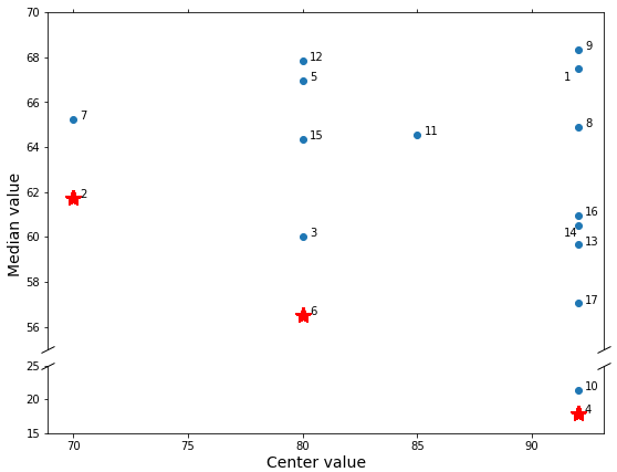
Figure 8: Identification of Pareto-optimality solutions for the given network of Example 5.

2.4 Adding efficiency to the generalized-center problem.

In our prior analysis, we observed peculiarities in the solutions of the generalized-center concerning to the center and median functions. When the search domain for the generalized-center is confined to the set $\mathcal{PO}^{\alpha}_{2}$, it aligns with the least efficient center network. We study the effect of imposing constraints that limit the degree of inefficiency of the sub-network, by adding the following constraint:

$$F_{m}(\mathcal{S}^{*})\leq(1+\Delta)\,F_{m}(\mathcal{S}_{m}),\quad\text{ with }\Delta\geq 0.$$ (2.15)

By setting $\Delta=0$, we ensure that the median objective value in $\mathcal{S}^{*}$ is precisely equivalent to that in $\mathcal{S}_{m}$. Note that, by definition, $F_{m}(\mathcal{S}_{m})\leq F_{m}(\mathcal{S}),\forall,\mathcal{S}\in\mathbfcal{N}^{\alpha}$. When $\Delta\in(0,1)$, we concede a certain percentage of efficiency. In other words, the median objective value in the optimal solution network can exceed the median network value by a specified percentage. Lastly, if $\Delta\geq 1$, we permit the efficiency value to surpass that of the median network by a multiple.

We have studied different solution concepts for the network design problem under the lens of two key solution concepts: the median and the center. We have further discussed the Pareto-optimality set of these two objectives. We have studied the weaknesses under this lens of the generalized-center. In Section 4, we will show that the generalized-center in the presence of efficiency constraints such as 2.15 are not dominated under some other inequality measures such as the mean absolute deviation and the percentage of the O/D pairs served by the network to be constructed (see Mesa et al. (2003)).

2.5 Complexity discussion

The problems addressed in this paper are NP-hard. The objective functions of the $\lambda$-cent-dians and generalized center problems are linear combinations of the median and center functions. Thus, if both network design problems are NP-hard, then so are the $\lambda$-cent-dians and generalized center problems. In Propositions 5 and 6 we show that the p-median and p-center problems are special cases of median and center subnetwork problems. It is known that the p-median and p-center problems are NP-hard (see Kariv & Hakimi (1979a) and Kariv & Hakimi (1979b)).

Proposition 5.

The problem of finding a median subnetwork from a given network is NP-hard.

Proof.

We show that the p-Median Problem reduces to the problem of finding a median subnetwork.

Given a set $I$ of demand nodes, let denote by $d_{ij}\geq 0$ the distance between demand nodes $i,j\in I$, with $d_{ij}=0$, if $i=j$. The decision version of the p-Median problem consists in determining a subset $S\subseteq I$, such that (i) $|S|=p$, and (ii) $f_{m}(S)=\sum_{i\in I}\min_{j\in S}d_{ij}\leq K$.

The corresponding median subnetwork problem is obtained as follows.

Regarding the network, the node set $N=I\cup\{t\}$ and the edge set $E=\{(i,j):i,j\in I\cup\{t\}\}$. The costs $c_{it}=1$ for all nodes $i\in I$ and the cost of all the other edges (linking pairs of nodes $i,j\in I$) are equal to zero. The cost $b_{i}=0$ for all nodes $i\in I\cup\{t\}$. The length of the edges linking pair of nodes i and j from $I$ is given by $d_{ij}$ and we set $d_{it}=0$ for all $i\in I$.

The set of O/D pairs $W=\{(i,t):i\in I\}$ and each pair $w$ has a unit demand, $g^{w}=1$ and an arbitrary large private utility, $u^{w}=M$. It is easy to see that there exists a subset $S$ satisfying the above conditions (i) and (ii) if and only if there exists a subnetwork $S^{\prime}$ with a cost lower than or equal to $\alpha C_{total}=p$ and $F_{m}(S^{\prime})\leq K$. The network $S^{\prime}$ contains all nodes in $I\cup\{t\}$, all edges between pairs of nodes in $I$ and $p$ edges linking the nodes in $S$ to the destination node $t$. Further, $f_{m}(S)=F_{m}(S^{\prime})$. ∎

Proposition 6.

The problem of finding a center subnetwork from a given network is NP-hard.

Proof.

The p-center problem reduces to the center subnetwork problem. The reduction is exactly the same as that of the median version given in the previous proposition. ∎

Propositions 6 and 7 are evidence that solving this family of problems is hard. In consequence, in the rest of the article, we focus on methods based on mathematical programming formulations to solve this problem at optimality.

3 Problem formulations

In this section, we present mixed-integer linear formulations for the $\lambda$-cent-dian problem as defined in equation (2.4). Initially, we introduce a mixed-integer formulation suitable for instances where $\lambda\in[0,1]$. However, this formulation becomes invalid for cases where $\lambda>1$. Consequently, we propose a general-case representation as a bilevel problem formulation. This includes consideration of the limit as $\lambda\rightarrow\infty$, which aligns with a valid formulation for the generalized-center problem (see equation (2.5)). We then convert the bilevel problem into a single-level valid formulation. Additionally, we integrate the criterion for efficiency, as specified in equation (2.15), into our proposed models. Finally, we describe a method for obtaining the set $\mathcal{PO}^{\alpha}_{2}$ by solving two distinct linear formulations.

3.1 Problem formulation for $\lambda\in[0,1]$

We present a mixed-integer formulation of the $\lambda$-cent-dian problem, (CD) in what follows, for the case $\lambda\in[0,1]$ by introducing the design variables $y_{i}$ and $x_{e}$ that represent the binary design decisions of constructing node $i$ and edge $e$, respectively. For each $w\in W$, a set of flow variables $f^{w}_{a},\,a\in A$ is used to model a path between $w^{s}$ and $w^{t}$, if possible. Variable $f_{a}^{w}$ takes value $1$ if arc $a$ belongs to the path from $w^{s}$ to $w^{t}$, and $0$ otherwise. We consider an extra artificial arc $r=(w^{s},w^{t})$ and its corresponding flow variable $f^{w}_{r}$ to model the alternative mode. Variable $f^{w}_{r}$ takes value $1$ if the length of the shortest path from $w^{s}$ to $w^{t}$ in the designed subgraph is larger than $u^{w}$ and 0 otherwise. In other words, $f^{w}_{r}=1$ represents the binary decision of the demand taking the alternative mode. Finally, we consider the continuous variable $\gamma^{max}$, taking the value of the maximum distance of any O/D pair in the graph.

$$\mbox{(CD)}\quad\min\, \quad\lambda\gamma^{max}+(1-\lambda)\frac{1}{G}\sum_{w\in W}g^{w}\left(\sum_{a\in A^{w}}d_{a}\,f_{a}^{w}+u^{w}\,f_{r}^{w}\right)$$ (3.1)

s.t. $$\quad\sum\limits_{e\in E}c_{e}\,x_{e}+\sum\limits_{i\in N}b_{i}\,y_{i}\leq\alpha\,C_{total},$$ (3.2)

$$\quad x_{e}\leq y_{i},\hskip 247.53888pte\in E,\,i\in e,$$ (3.3)

$$\quad f_{r}^{w}+\sum_{a\in\delta_{w}^{+}(i)}f^{w}_{a}-\sum_{a\in\delta_{w}^{-}(i)}f^{w}_{a}=\begin{cases}1,&\text{if $i=w^{s}$},\\ -1,&\text{if $i=w^{t}$},\\ 0,&\text{otherwise},\end{cases}\hskip 15.6491ptw=(w^{s},w^{t})\in W,\,i\in N,$$ (3.4)

$$\quad f_{a}^{w}+f_{\hat{a}}^{w}\leq x_{e},\hskip 128.0374ptw\in W,\,a=(i,j)\in A^{w}:e=\{i,j\},$$ (3.5)

$$\quad\sum_{a\in A}d_{a}\,f_{a}^{w}+u^{w}\,f_{r}^{w}\leq\gamma^{max},\hskip 190.63338ptw\in W,$$ (3.6)

$$\quad x_{e},\,y_{i},\,f_{r}^{w},\,f_{a}^{w}\,\in\{0,1\},\quad\gamma^{max}\geq 0,\hskip 59.75095pti\in N,\,e\in E,\,a\in A,\,w\in W.$$ (3.7)

The objective function (3.1) to be minimized represents a convex combination between the center and the median objectives. Constraint (3.2) limits the total construction cost, being $\alpha\in(0,1]$. Constraint (3.3) ensures that if an edge is constructed, then its terminal nodes are constructed as well. For each pair $w$, constraints (3.4), guarantee flow conservation and demand satisfaction. Constraints (3.5) are named capacity constraints and force each edge to be used in at most one direction by each O/D pair whenever such edge is built. Constraints (3.6), referenced as maximum distance constraints, determines the maximum length of the shortest path between all pairs $w=(w^{s},w^{t})\in W$. The structure of the objective function ensures that variable $f_{r}^{w}$ assumes the value of $0$ only if a path between $w^{s}$ and $w^{t}$ exists with a length not exceeding $u^{w}$ in the prospective network. This path is symbolized by the variables $f_{r}^{w}$. Subsequently, $\gamma^{max}$ denotes the greatest $\ell_{\mathcal{S}}(w)$ within the set $W$. Finally, constraints (3.7) specify that all variables are binary, with the exception of variable $\gamma^{max}$.

For $\lambda\in[0,1)$, the objective function of the above formulation is composed of two non-negative coefficients ($\lambda$ and $(1-\lambda)$) that multiply increasing functions of travel times. In consequence, at any optimal solution, the demand always chooses the shortest path without the necessity of enforcing this condition. That is, optimal solution vectors $\boldsymbol{f}^{w}$ correspond to shortest paths in the solution network.

For $\lambda\geq 1$, the variables $f$ are no longer mandated to represent the shortest path. In the specific instance where $\lambda=1$, the solution sub-network of (CD) serves as a center of the network, preserving the center objective’s correctness. This suggests that (CD) remains a valid formulation for the center problem. However, when $\lambda>1$, this no longer holds true. As the term ($1-\lambda$) is negative, each O/D pair $w$ within this formulation will opt for an arbitrary path between $w^{s}$ to $w^{t}$ in the designed network. We illustrate this situation in Example $6$.

Example 6

Let us consider the same potential network and its associated data from Example $3$ with $\alpha\,C_{total}=100$ and $\lambda=50\cdot 10^{4}$. One of the optimal $\lambda$-cent-dian solution networks for formulation (CD) is

with the flow vector $f^{w}_{r}=1,\,w\in\{(1,2),(4,1)\}$ and $f^{w}_{r}=0,\,w\in\{(2,6)\}$. The path selected for $w=(2,6)$ is $[2,1,3,5,6]$ but the path $[2,3,5,6]$ is shorter than the selected one. Besides, this solution does not assign the pairs $(1,2)$ and $(4,1)$ to the existing paths in the network although they are shorter than the utilities $u^{(1,2)}=92$ and $u^{(4,1)}=92$. Then, the objective value is $92-91.90$. Nevertheless, this is not the solution network that should be obtained, as you can check in Example 3.

3.2 Problem formulation for $\lambda>1$. General problem formulation

We introduce a bilevel formulation to ensure that each $w$ selects the shortest path in the solution network for any value of $\lambda\geq 0$, especially for cases where $\lambda>1$. This is called the bilevel $\lambda$-cent-dian formulation and is denoted as (BCD).

$$\mbox{(BCD)}\,\min \quad\lambda\gamma^{max}+(1-\lambda)\frac{1}{G}\sum_{w\in W}g^{w}\left(\sum_{a\in A^{w}}d_{a}\,f_{a}^{w}+u^{w}\,f_{r}^{w}\right)$$ (3.8)

s.t. $$\quad\sum\limits_{e\in E}c_{e}\,x_{e}+\sum\limits_{i\in N}b_{i}\,y_{i}\leq\alpha\,C_{total},$$ (3.9)

$$\quad x_{e}\leq y_{i},\hskip 241.84842pte\in E,\,i\in e,$$ (3.10)

$$\quad\sum_{a\in A}d_{a}\,f_{a}^{w}+u^{w}\,f_{r}^{w}\leq\gamma^{max},\hskip 179.25244ptw\in W,$$ (3.11)

$$\quad\boldsymbol{f}^{\prime w}\in sol(\mbox{(F)}^{w}),\hskip 230.46748ptw\in W,$$ (3.12)

$$\quad x_{e},\,y_{i},\,f_{a}^{w}\,\in\{0,1\},\quad\gamma^{max}\geq 0,\hskip 68.28644pti\in N,\,e\in E,\,a\in A,\,w\in W,$$ (3.13)

where

$$\mbox{(F)}^{w}=\arg\min\limits_{\boldsymbol{f}^{\prime}}\left\{\left(\sum_{a\in A^{w}}d_{a}\,f_{a}^{\prime w}+u^{w}\,f_{r}^{\prime w}\right):\,\text{ s.t.}\left.\begin{cases}\text{const.}(\ref{cons:flow})-(\ref{cons:capacity}),\kern-28.45274pt\\ f_{r}^{\prime w},f_{a}^{\prime w}\,\in\{0,1\},\,a\in A^{w}\kern-8.5359pt\end{cases}\right\}\right\}.$$ (3.14)

The bilevel formulation (BCD) consists in an upper-level task that designs a network to minimize the $\lambda$-cent-dian function, and a lower-level task for each O/D pair $w\in W$ that aims to identify the shortest path between $w^{s}$ and $w^{t}$ within the designed network. The optimal solutions for the lower-level problems are articulated in equation (3.14) and are denoted as $\mbox{(F)}^{w}$.

We reformulate the bilevel problem (BCD) as a single-level problem by imposing the optimality conditions of each problem (F)^w as constraints of the upper-level problem. To do so, we consider the dual of each problem (F)^w, denoted by (DF)^w:

$$\mbox{(DF)}^{w}\quad\max\limits_{\boldsymbol{\alpha},\boldsymbol{\sigma}} \quad\alpha^{w}_{w^{s}}-\sum_{e\in E}x_{e}\,\sigma^{w}_{e}$$ (3.15)

s.t. $$\quad\alpha^{w}_{i}-\alpha^{w}_{j}-\sigma^{w}_{e}\leq d_{a},\hskip 65.44142pta=(i,j)\in A^{w}:e=\{i,j\},$$ (3.16)

$$\quad\alpha^{w}_{w^{s}}\leq u^{w},$$ (3.17)

$$\quad\sigma^{w}_{e}\geq 0,\hskip 199.16928pte\in E^{w}.$$ (3.18)

As it is clear from the context, we omit the index $w$. Variables $\alpha_{i},i\in N$, are the dual variables related to the flow constraints (3.4) and $\sigma_{e},\,e\in E$, are the dual variables corresponding to the capacity constraints (3.5). Given that the set of flow constraints contains one linear dependent constraint, we set $\alpha_{w^{t}}=0$.

Since $d_{a}$ and $u^{w}$ are positive parameters, each $(F)^{w}$ has optimal finite solutions. In consequence, by strong duality, a feasible vector $\boldsymbol{f}^{w}$ for (F)^w is optimal if and only if there exist feasible vectors $\boldsymbol{\alpha}$ and $\boldsymbol{\sigma}$ for $\mbox{(DF)}^{w}$ such that:

$$\sum\limits_{a\in A}d_{a}\,f_{a}+u\,f_{r}=\alpha_{w^{s}}-\sum\limits_{e\in E}x_{e}\,\sigma_{e}.$$

Then, (BCD) can be cast as a single-level non-linear optimization problem:

$$\mbox{(BCD\_R)}\,\,\min \quad\lambda\gamma^{max}+(1-\lambda)\frac{1}{G}\sum_{w\in W}g^{w}\left(\sum_{a\in A^{w}}d_{a}\,f_{a}^{w}+u^{w}\,f_{r}^{w}\right)$$

s.t. $$\quad\sum\limits_{e\in E}c_{e}\,x_{e}+\sum\limits_{i\in N}b_{i}\,y_{i}\leq\alpha\,C_{total},$$

$$\quad x_{e}\leq y_{i},\quad\quad e\in E,\,i\in e,$$

$$\quad\sum_{a\in A}d_{a}\,f_{a}^{w}+u^{w}\,f_{r}^{w}\leq\gamma^{max},\hskip 182.09746ptw\in W,$$

$$\quad f_{r}^{w}+\sum_{a\in\delta_{w}^{+}(i)}f^{w}_{a}-\sum_{a\in\delta_{w}^{-}(i)}f^{w}_{a}=\begin{cases}1,&\text{if $i=w^{s}$},\\ 0,&\text{if }i\notin\{w^{s},w^{t}\},\end{cases}\quad w=(w^{s},w^{t})\in W,\,i\in N,$$

$$\quad f^{w}_{a}+f^{w}_{\hat{a}}\leq x_{e},\hskip 119.50148ptw\in W,\,e=\{i,j\}\in E^{w}:a=(i,j),$$

$$\quad\alpha^{w}_{i}-\alpha^{w}_{j}-\sigma^{w}_{e}\leq d_{a},\hskip 96.73918ptw\in W,\,a=(i,j)\in A^{w}:e=\{i,j\},$$

$$\quad\alpha^{w}_{w^{s}}\leq u^{w},\hskip 258.92024ptw\in W,$$

$$\quad\sum\limits_{a\in A^{w}}d_{a}\,f^{w}_{a}+u^{w}\,f^{w}_{r}=\alpha^{w}_{w^{s}}-\sum\limits_{e\in E^{w}}x_{e}\,\sigma^{w}_{e},\hskip 113.81102ptw\in W,$$ (3.19)

$$\quad x_{e},\,y_{i},\,f_{r}^{w},\,f_{a}^{w}\,\in\{0,1\},\quad\gamma^{max},\,\sigma^{w}_{e}\geq 0,\hskip 25.6073pti\in N,\,e\in E,\,a\in A,\,w\in W.$$ (3.20)

The model above is a mixed integer non-linear problem that can be linearized by replacing the non-linear terms in (3.19). We introduce the set of variables $\xi^{w}_{e}$, representing the product $x_{e}\,\sigma^{w}_{e}$ and we linearize them by using the following McCormick inequalities (see McCormick (1976)):

$$\xi_{e}\leq x_{e}\Sigma_{e},$$ (3.21)

$$\xi_{e}\leq\sigma_{e},$$ (3.22)

$$\xi_{e}\geq\sigma_{e}-\Sigma_{e}(1-x_{e}),$$ (3.23)

$$\xi_{e}\geq 0,$$ (3.24)

where $\Sigma_{e}$ is an upper bound of $\sigma_{e}$.

The computational efficiency of the McCormick reformulation relies on the availability of tight bounds of $\sigma^{w}_{e}$. To get such bounds, we consider the assumption that for each $w\in W$, $d_{\mathcal{N}}(w)\leq u^{w}$, meaning that there exists a possible path to be designed for each pair that improves its private utility. This is not a restrictive assumption since a pair not satisfying this condition will always prefer the private mode and can be eliminated from the analysis. Under this mild assumption, Propositions 7 and 8 establish an efficient way to compute the best bound on the dual variables $\sigma^{w}_{e}$.

Proposition 7.

The quantity $\Sigma^{w}_{e}=u^{w}-d_{\mathcal{N}}(w)$ is a valid bound for $\sigma_{e}^{w}$ in (BCD_R).

Proof.

For each $w\in W$, rewriting (3.19), we have that

$$\sum\limits_{e\in E^{w}}x_{e}\,\sigma^{w}_{e}=\alpha^{w}_{w^{s}}-\left(\sum\limits_{a\in A^{w}}d_{a}\,f^{w}_{a}+u^{w}\,f^{w}_{r}\right).$$

Using (3.17) and that $\sum\limits_{a\in A^{w}}d_{a}\,f^{w}_{a}+u^{w}\,f^{w}_{r}\geq d_{\mathcal{N}}(w)$, then

$$\sum\limits_{e\in E^{w}}x_{e}\,\sigma^{w}_{e}\leq u^{w}-d_{\mathcal{N}}(w).$$

Thus, we can conclude that $\sigma^{w}_{e}\leq u^{w}-d_{\mathcal{N}}(w)$. ∎

Proposition 8.

The bound given in Proposition 7 is tight.

Proof.

Let us fix a pair $w\in W$ and consider the particular situation for which there exists $e=\{w^{s},w^{t}\}\in E^{w}\subseteq E$ and $d_{\mathcal{N}}(w)=d_{(w^{s},w^{t})}$. Let us suppose that there exists a better bound for $\sigma_{\{w^{s},w^{t}\}}^{w}$ than $u^{w}-d_{\mathcal{N}}(w)$. That is, $\sigma_{\{w^{s},w^{t}\}}^{w}\leq u^{w}-d_{\mathcal{N}}(w)-\epsilon$. By (3.16), $\alpha_{w_{s}}^{w}\leq d_{a}+\sigma_{\{w^{s},w^{t}\}}^{w}\leq u^{w}-\epsilon$. Then, according to (3.19),

$$\alpha_{w_{s}}^{w}=\sum_{a\in A^{w}}d_{a}\,f^{w}_{a}+u^{w}\,f^{w}_{r}+\sum_{e\in E^{w}}x_{e}\,\sigma_{e}^{w}\leq u^{w}-\epsilon.$$ (3.25)

In order to satisfy the previous inequality, $f^{w}_{r}$ has to be set to $0$, which forces a solution network to have a path for $w$ (the corresponding flow variables take value equal to $1$). This situation can result in an infeasible solution by (3.14) if the length of the assigned path is larger than its $u^{w}$ or even if there is no path.

Let us show it with a small example. Let $\mathcal{N}$ be the following potential network.

Origin	Destination	$u^{w}$	$g^{w}$
1	2	24	181
1	4	34	168
2	4	20	43
3	2	32	121

Being $\lambda=20$ and $\alpha\,C_{total}=63$, the optimal solution for (Bilevel-CD) is

which means that $x_{\{1,2\}}=0$. By Proposition 8, it is set $f_{r}^{(1,2)}=0$, which forces to assign $w$ to the solution network. This solution network contains a path for $w$ but it is larger than its $u^{w}$, which results in an infeasibility by (3.14) for not taking the optimal mode. ∎

To conclude, as we discussed, the generalized-center tends to be suboptimal in efficiency and is not necessarily characterized as a center network. In Section 2.4, we introduced a constraint to enhance the efficiency of the generalized-center solution. Specifically, for cases where $\lambda>1$, we augment the (BCD) formulation with the following constraint:

$$\frac{1}{G}\sum_{w\in W}g^{w}\left(\sum_{a\in A^{w}}d_{a}\,f_{a}^{w}+u^{w}\,f_{r}^{w}\right)\leq(1+\Delta)F_{m}(\mathcal{S}_{m}),$$ (3.26)

being $F_{m}(\mathcal{S}_{m})$ the objective value of the median network (the objective value for (CD) for $\lambda=0$).

3.3 An algorithm to describe the set $\mathcal{PO}^{\alpha}_{2}$

Proposition 4 proves that the set $\mathcal{PO}^{\alpha}_{2}$ can be exhaustively described as a function of $\lambda\in(0,1)$ with minimization of the weighted function $\bar{H}_{\lambda}(\,\cdot\,)$. In the case of a non-unique optimal solution, we select the one that has minimum $H_{\lambda}(\,\cdot\,)$ value. That is, firstly, to minimize $\bar{H}_{\lambda}(\,\cdot\,)$ we solve the problem

$$\quad\min\, \quad\mu$$ (3.27)

s.t. $$\quad\mu\geq\lambda\,F_{c}(\mathcal{S}),$$ (3.28)

$$\quad\mu\geq(1-\lambda)\,F_{m}(\mathcal{S}),$$ (3.29)

$$\quad\mathcal{S}\in\mathcal{N}^{\alpha},$$ (3.30)

$$\quad\mu\geq 0.$$ (3.31)

Then, being $V^{*}$ the objective value of the problem formulation (3.27)-(3.31), the following second problem is solved for regulation purposes:

$$\quad\min\, \quad\lambda F_{c}(\mathcal{S})+(1-\lambda)F_{m}(\mathcal{S})$$ (3.32)

s.t. $$\quad\lambda\,F_{c}(\mathcal{S})\leq V^{*},$$ (3.33)

$$\quad(1-\lambda)\,F_{m}(\mathcal{S})\leq V^{*},$$ (3.34)

$$\quad\mathcal{S}\in\mathcal{N}^{\alpha},$$ (3.35)

In terms of sets $N$, $E$ and $W$, the previous formulations are equivalent to the following ones

$$\mbox{(MCD\_1)}\quad\min\, \quad\mu$$ (3.36)

s.t. $$\quad\mu\geq\lambda\,\left(\sum_{a\in A^{w}}d_{a}\,f_{a}^{w}+u^{w}\,f_{r}^{w}\right),\hskip 85.35826ptw\in W,$$ (3.37)

$$\quad\mu\geq(1-\lambda)\,\frac{1}{G}\sum_{w\in W}g^{w}\left(\sum_{a\in A^{w}}d_{a}\,f_{a}^{w}+u^{w}\,f_{r}^{w}\right),$$ (3.38)

$$\quad\mu\geq 0,$$ (3.39)

$$\quad\text{constraints }\eqref{cons:budget},\eqref{cons:location},\eqref{cons:flow},\eqref{cons:capacity},\eqref{cons:var}$$ (3.40)

$$\mbox{(MCD\_2)}\quad\min\, \quad\lambda\left(\sum\limits_{a\in A^{w}}d_{a}\,f_{a}^{w}+u^{w}\,f_{r}^{w}\right)+(1-\lambda)\frac{1}{G}\sum\limits_{w\in W}g^{w}\left(\sum\limits_{a\in A^{w}}d_{a}\,f_{a}^{w}+u^{w}f_{r}^{w}\right)$$ (3.41)

s.t. $$\quad 0\leq V^{*}-\lambda\,\left(\sum_{a\in A^{w}}d_{a}\,f_{a}^{w}+u^{w}\,f_{r}^{w}\right),\hskip 56.9055ptw\in W,$$ (3.42)

$$\quad 0\leq V^{*}-(1-\lambda)\,\frac{1}{G}\sum_{w\in W}g^{w}\left(\sum_{a\in A^{w}}d_{a}\,f_{a}^{w}+u^{w}\,f_{r}^{w}\right),$$ (3.43)

$$\quad\mu\geq 0,$$ (3.44)

$$\quad\text{constraints }\eqref{cons:budget},\eqref{cons:location},\eqref{cons:flow},\eqref{cons:capacity},\eqref{cons:var}.$$ (3.45)

To obtain all the existing correspondences between all the solution networks in $\mathcal{PO}^{\alpha}_{2}$ and its associated value $\lambda\in(0,1)$, we can use the bisection method for $\lambda$ parameter in the interval $(0,1)$. For that, at each iteration, the current solution network obtained is compared with the last two solutions computed previously.

4 Quality of the solutions with a numerical illustration

In this section, we illustrate the quality of the solutions for the different solution concepts developed in Section 2 through an example. The instance used in this part has been generated randomly in the same manner as in Section 5.2, being the network resultant of a planar graph consisting of 20 nodes, shown in Figure 9.

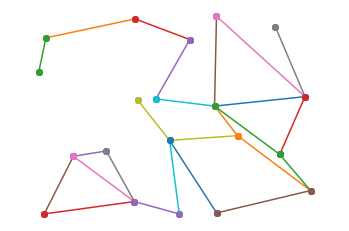
Figure 9: Potential graph used in Section 4.

The quality of the solution $\mathcal{S}$ is presented in terms of:

• the minimum length of a path among all the pairs: $\ell_{\mbox{min}}({\mathcal{S}})=\min_{w}\ell_{\mathcal{S}}(w)$,

• the maximum length of a path among all the pairs: $\ell_{\mbox{max}}({\mathcal{S}})=\min_{w}\ell_{\mathcal{S}}(w)$,

• the average length of the paths: $\overline{\ell}(\mathcal{S})=\frac{1}{|W|}\sum_{w}\ell_{\mathcal{S}}(w)$,

• the mean absolute difference of the path’s length:
  MAD$(\mathcal{S})=\frac{1}{2}\sum\limits_{w\in W}\sum\limits_{\begin{subarray}{c}w^{\prime}\in W:\\ w\neq w^{\prime}\end{subarray}}g^{w}g^{w^{\prime}}|\ell_{\mathcal{S}}(w)-\ell_{\mathcal{S}}(w^{\prime})|$,

• the O/D pairs served refers to the number of O/D pairs that prefer the solution network over the one provided by the private mode. This is denoted by O/D%.

$\lambda$	$\Delta$ (%)	$\ell_{\mbox{min}}$	$\ell_{\mbox{max}}$	$\overline{\ell}$	MAD	O/D%
0	-	4	100	45.037	12.351	28.187
0.25	-	4	100	45.037	12.351	28.187
0.5	-	4	96	47.149	12.375	27.516
0.75	-	4	96	47.149	12.375	27.516
1	-	4	96	47.383	12.187	6.375
1	0	4	100	45.037	12.351	28.187
1	3	4	100	45.981	12.322	24.832
1	5	4	96	47.149	12.375	23.154
1	10	4	96	47.383	12.187	8.389
1	15	4	96	47.383	12.187	8.389
500	-	4	96	48.655	12.535	21.476
500	0	4	100	45.037	12.351	28.187
500	3	5	100	46.386	12.279	24.832
500	5	4	96	47.283	12.859	26.174
500	10	4	96	48.655	12.535	21.476
500	15	4	96	48.655	12.535	21.476
lex	-	4	96	47.149	12.375	27.516

Table 6: Quality of solutions for $\lambda$-cent-dian and generalized-center problems using a random instance with $|N|=20$ and $\alpha=0.4$.

Table 6 summarizes the different values of the performance index mentioned above and is arranged as follows. The first set of rows corresponds to the $\lambda$-cent-dian problem for $\lambda\in\{0,0.25,0.5,0.75\}$. Secondly, we consider the center problem ($\lambda=1$). In the third set of rows, the approximation of the generalized-center concept with $\lambda=500$ is considered. For the center and generalized-center problems, the effect of adding the efficiency constraint (2.15) with $\Delta\in\{0\%,3\%,5\%,10\%,15\%\}$ is considered. In the last row, we consider the lexicographic cent-dian (2.10). Note that for the particular case with $\lambda=1$ and $\Delta=0$, we are solving the inverse lexicographic problem: first, we solve the median problem by optimizing $F_{m}(\cdot)$, and subsequently, we seek the best center among the optimal solutions of the median. We have solved formulations (CD) and (BCD) exposed in Section 3 with the direct use of Python 3.8 and the optimization solver CPLEX 12.10.

First, note that only two different solutions are obtained by solving the problem for range $\lambda\in(0,1)$. These solutions belong to the set $\mathcal{PO}_{2}^{\alpha}$ (Remark 2). In the first four rows of Table 6 is noted the compromise between the median and the center objectives. For $\lambda\in\{0,0.25\}$, the maximum travel time ($\ell_{\mbox{max}}$) is 100, which decreases to 96 when $\lambda\in\{0.5,0.75\}$ is considered. As it is expected, the opposite effect is observed with the median objective $\overline{\ell}(\mathcal{S})$, which increases from 45.037 to 47.149. We observe the same effect with the percentage of O/D pairs served.

For $\lambda=1$ and $\Delta=0$, the formulation seeks the median solution with the minimum center value. Similarly, when $\lambda=500$ and $\Delta=0$, the optimal solution corresponds to the median network with the lowest generalized-center value. These solution networks are exactly the solution for the configuration with $\lambda\in\{0,0.25\}$. Comparing configurations with $\Delta>0$ for both $\lambda=1$ and $\lambda=500$, we observe that with, $\lambda=1$ the average travel time increases, being greater than in the median solution (as expected) and smaller than in the generalized-center solutions. Additionally, in both cases, employing the efficiency constraint results in more O/D pairs being served than when it is not used, provided that the parameter $\Delta$ is not excessively large. Furthermore, for a fixed value of $\Delta$, the percentage of O/D pairs served by the generalized-center solution is either greater than or equal to that served by the center solution. Regarding the mean absolute difference measure, no distinct trend can be identified; we simply observe that, in this case, the center solution has the lowest value for this measure.

Besides, we observe that comparing the center solutions between them, there are some dominated ones. More specifically, the center solution without the efficiency constraint ($\Delta$= - ) is completely dominated by the solution where this constraint is used with $\Delta=15$. On the other hand, a similar situation arises when comparing the generalized-center solutions among themselves.

Making a general comparison, we highlight that there are some generalized-center solutions non-dominated by the rest. The generalized-center solution with $\Delta=3$ has smaller values of M.A.D than any of $\lambda$-cent-dian solutions with $\lambda<1$. If we compare it with the center solutions, we see that two situations can occur: i) the center solution has a smaller M.A.D value but a bigger average value and a lower percentage of demand covered, or ii) if the center has a worse M.A.D value, then it also has better values for some of the inequality measures evaluated.

In a general comparison, we emphasize that some generalized-center solutions are not dominated by the rest of the solutions in Table 6. The generalized-center solution with $\Delta=3$ has smaller values of M.A.D than any of the $\lambda$-cent-dian solutions with $\lambda<1$. When comparing it with the center solutions, two situations may arise: i) the center solution has a smaller M.A.D value but a larger Average value and a lower percentage of demand covered, or ii) if the center solution has a worse M.A.D value, it also has better values for some of the inequality measures evaluated.

5 Algorithmic discussion for $\lambda\in[0,1]$

In this section we present how for $\lambda\in[0,1]$, the formulation (CD) possesses the suitable separable structure needed for a Benders decomposition approach. Indeed, when the design variables of (CD), namely $x$, $y$ and $\gamma^{max}$, are fixed, the problem can be divided into $|W|$ sub-problems. Each of these sub-problems establishes the flow variables $f^{w}$ as a linear problem by relaxing their integrality condition.

However, it is important to note that this property is not present in (BCD), where the flow variables must also meet a non-convex optimality condition. Since (CD) is not a valid formulation for $\lambda>1$, the Benders decomposition developed in this section is only appropriate for $\lambda\in[0,1]$.

5.1 Benders Decomposition with facet-defining cuts for $\lambda\in[0,1]$

Formulation (CD) involves a large number of flow variables when the set of O/D pairs is extensive. To address this issue, we explore a stabilized Benders decomposition based on the concepts presented in Conforti & Wolsey (2019) to generate facet-defining cuts. This method has been previously examined and developed for covering problems in Cordeau et al. (2019) and Bucarey et al. (2022). We investigate an implementation of the branch-and-Benders-cut algorithm (B&BC) for the case $\lambda\in[0,1]$.

To generate such cuts, we first need to relax the integrality condition on the flow variables $f^{w}_{a}$ and $f^{w}_{r}$. Proposition 9 shows that this can be done without loss of generality. Let (CD_R) denote the formulation (CD) in which constraints $f_{a}^{w}\in\{0,1\},w\in W,a\in A\cup\{r\}$ are replaced by non-negativity constraints, i.e.

$$f^{w}_{a}\geq 0,w\in W,a\in A\cup\{r\}.$$ (5.1)

Let $Q$ be a set of points $(\boldsymbol{x},\boldsymbol{z})\in\mathbb{R}^{n}\times\mathbb{R}^{m}$. Then, the projection of $Q$ onto the $x$-space, denoted by $Proj_{x}(Q)$, is the set of points given by: $Proj_{\boldsymbol{x}}(Q)=\{\boldsymbol{x}\in\mathbb{R}^{m}:(\boldsymbol{x},\boldsymbol{z})\in Q\text{ for some }\boldsymbol{z}\in\mathbb{R}^{n}\}.$ Let us denote by $\mathcal{F}(CD)$ the set of feasible points of formulation $(CD)$.

Proposition 9.

The projections of (CD) and (CD_R) onto the $\boldsymbol{f}$-space coincide.

$$Proj_{\boldsymbol{x},\boldsymbol{y},\boldsymbol{\gamma^{max}}}(\mathcal{F}(CD))=Proj_{\boldsymbol{x},\boldsymbol{y},\boldsymbol{\gamma^{max}}}(\mathcal{F}(CD\_R)).$$

Proof.

First, $\mathcal{F}(CD)\subseteq\mathcal{F}(CD\_R)$ implies $Proj_{\boldsymbol{x},\boldsymbol{y},\boldsymbol{\gamma^{max}}}(\mathcal{F}(CD))\subseteq Proj_{\boldsymbol{x},\boldsymbol{y},\boldsymbol{\gamma^{max}}}(\mathcal{F}(CD\_R))$. Second, let $(\boldsymbol{x},\boldsymbol{y},\boldsymbol{\gamma^{max}})$ be a point belonging to $Proj_{\boldsymbol{x},\boldsymbol{y},\boldsymbol{\gamma^{max}}}(\mathcal{F}(CD\_R))$. Due to the structure of the objective function, every O/D pair will select one of the two modes, the shortest one. That is, $f^{w}_{r}$ will take the value of $0$ or $1$. If $f_{r}^{w}=1$ then $\boldsymbol{f}^{w}=0$. In the case where $f_{r}^{w}=0$, there exists a flow $f^{w}_{a}\geq 0$ satisfying (3.4) and (3.5) that can be decomposed into a convex combination of flows on paths from $w^{s}$ to $w^{t}$ plus possibly some cycles. Further, $x_{e}=1$ for all edges belonging to these paths which have the same length. Given that the flow $f_{a}^{w}$ also satisfies (3.6), then a flow of value $1$ on one of the paths in the convex combination must satisfy this constraint. Hence, by taking $f_{a}^{w}$ equal to $1$ for the arcs belonging to this path and to $0$ otherwise, we show that $(\boldsymbol{x},\boldsymbol{y},\boldsymbol{\gamma^{max}})$ also belongs to $Proj_{\boldsymbol{x},\boldsymbol{y},\boldsymbol{\gamma^{max}}}(\mathcal{F}(CD))$. ∎

Based on Proposition 9, we propose a Benders decomposition where variables $f^{w}_{a}$ and $f^{w}_{r}$ are projected out from the model and replaced by Benders facet-defining cuts, generated on-the-fly. Following the Benders decomposition Theory, since flow variables appear in the objective function of (CD), we have introduced an incumbent variable $\zeta^{w}$ for each O/D pair $w\in W$ to denote the expression $\sum_{a\in A^{w}}d_{a}\,f_{a}^{w}+u^{w}\,f_{r}^{w}$. Then, the master problem that we solve is

$$\mbox{(M\_CD)}\quad\min \quad\lambda\gamma^{max}+(1-\lambda)\frac{1}{G}\sum_{w\in W}g^{w}\zeta^{w}$$ (5.2)

s.t. $$\quad\sum\limits_{e\in E}c_{e}\,x_{e}+\sum\limits_{i\in N}b_{i}\,y_{i}\leq\alpha\,C_{total},$$ (5.3)

$$\quad x_{e}\leq y_{i},\hskip 142.26378pte\in E,\,i\in\{e^{s},e^{t}\},$$ (5.4)

$$\quad\zeta^{w}\leq\gamma^{max},\hskip 182.09746ptw\in W,$$ (5.5)

$$\quad+\{\mbox{Benders Cuts }(\boldsymbol{x},\boldsymbol{y},\boldsymbol{f},\boldsymbol{\zeta})\}.$$

$$\quad x_{e},\,y_{i}\,\in\{0,1\},\hskip 14.22636pt\gamma^{max},\zeta^{w}\geq 0,\hskip 25.6073pti\in N,\,e\in E,\,w\in W.$$ (5.6)

In Conforti & Wolsey (2019), the authors derive a cut-generating LP, the optimal solution of which almost surely induces a facet-defining Benders feasibility cut. To achieve this, it is necessary to generate a feasible solution in the interior of the convex hull of the feasible domain. Then, this cut-generating LP scheme finds the best cut that lies in the convex combination of such interior point and the point to be separated.

We obtain this interior point by first performing a preprocessing method to delete all the O/D pairs in the network that will not be served by any feasible solution of (CD). This is equivalent to eliminating all the O/D pairs that induce the implicit equality $f^{w}_{r}=1$. We then show that the convex hull of the resulting problem is full-dimensional by exposing a sufficient number of linearly independent feasible points. The average of such points is a point living in the interior of the convex hull of the feasible space.

We briefly describe the preprocessing scheme as follows. The first part involves constructing, for each pair $w\in W$, a subgraph $\mathcal{N}^{w}$ that includes only those nodes and edges present in any path from $w^{s}$ to $w^{t}$ that is shorter than or equal to $u^{w}$. In the second part, we identify the set of O/D pairs deemed too expensive to serve, denoted as $\bar{W}$. Specifically, these are pairs without a path from $w^{s}$ to $w^{t}$ in $\mathcal{N}^{w}$ that satisfies both: i) its building cost is less than $\alpha\,C_{total}$; and ii) its length is less than $u^{w}$. The mode choice decision for this set is fixed to $f_{r}^{w}=1$ and deleted from $W$. For a more detailed explanation, we refer to Bucarey et al. (2022).

The following Proposition 10 and its proof gives us a way to compute $|N|+|E|+|W|+2$ linearly independent points. In consequence, the average of these points is an interior point of the convex hull of $Proj_{\boldsymbol{x},\boldsymbol{y},\boldsymbol{\gamma^{max}},\boldsymbol{\zeta}}(\mathcal{F}(CD\_R))$.

Proposition 10.

After preprocessing, the convex hull of $Proj_{\boldsymbol{x},\boldsymbol{y},\boldsymbol{\gamma^{max}},\boldsymbol{\zeta}}(\mathcal{F}(\text{CD}\_R))$ is full-dimensional.

Proof.

See A. ∎

Given an interior point $(\boldsymbol{x}^{in},\boldsymbol{y}^{in},\boldsymbol{\gamma^{max}}^{in},\boldsymbol{\zeta}^{in})$ and an exterior point $(\boldsymbol{x}^{out},\boldsymbol{y}^{out},\boldsymbol{\gamma^{max}}^{out},\boldsymbol{\zeta}^{out})$, which is a solution to the LP relaxation of the current restricted master problem $Proj_{\boldsymbol{x},\boldsymbol{y},\boldsymbol{\gamma^{max}}}(\mathcal{F}(CD\_R))$, we generate a cut that induces either a facet or an improper face of the polyhedron defined by the LP relaxation of $Proj_{\boldsymbol{x},\boldsymbol{y},\boldsymbol{\gamma^{max}},\boldsymbol{\zeta}}\mathcal{F}(CD)$. We denote the difference $\boldsymbol{x}^{out}-\boldsymbol{x}^{in}$ by $\Delta\boldsymbol{x}$ and define $\Delta\boldsymbol{y}$, $\Delta\boldsymbol{\gamma^{max}}$, and $\Delta\boldsymbol{\zeta}$ analogously. The goal is to find the point furthest from the interior point that is feasible to the LP-relaxation of $Proj_{\boldsymbol{x},\boldsymbol{y},\boldsymbol{z}}\mathcal{F}(CD)$ and lies on the line segment between the interior point and the exterior point. This point takes the form $(\boldsymbol{x}^{sep},\boldsymbol{y}^{sep},\boldsymbol{\gamma^{max}}^{sep},\boldsymbol{\zeta}^{sep})=(\boldsymbol{x}^{out},\boldsymbol{y}^{out},\boldsymbol{\gamma^{max}}^{out},\boldsymbol{\zeta}^{out})-\mu(\Delta\boldsymbol{x},\Delta\boldsymbol{y},\Delta\boldsymbol{\gamma^{max}},\Delta\boldsymbol{\zeta})$. For each O/D pair $w$, we cast the cut-generation problem as:

$$\mbox{(SP)}^{w}\,\min\limits_{\boldsymbol{f},\mu} \,\mu$$ (5.7)

s.t. $$\,\,f_{r}+\sum\limits_{a\in\delta^{+}(i)}f_{a}-\sum\limits_{a\in\delta^{-}(i)}f_{a}=\begin{cases}1,&\text{if $i=w^{s}$},\\ 0,&\text{otherwise},\end{cases}\hskip 51.21504pti\in N,$$ (5.8)

$$\,\,f_{a}+f_{a^{\prime}}\leq x_{e}^{out}-\mu\,\Delta x_{e},\hskip 14.22636pte=\{i,j\}\in E:a=(i,j),a^{\prime}=(j,i),$$ (5.9)

$$\,\,\sum_{a\in A^{w}}d_{a}\,f_{a}+u\,f_{r}\leq\zeta^{out}-\mu\,\Delta\zeta,$$ (5.10)

$$\,\,0\leq\mu\leq 1,$$ (5.11)

$$\,\,f_{a}\geq 0,\hskip 219.08612pta\in A.$$ (5.12)

In order to obtain the Benders feasibility cut we solve its associated dual. Given that (SP)^w is always feasible ($\mu=1$ is feasible) and that its optimal value is lower bounded by 0, then, both (SP)^w and its associated dual problem have always finite optimal solutions. Whenever the optimal value of $\mu$ is 0, $(\boldsymbol{x}^{out},\boldsymbol{y}^{out},\boldsymbol{\gamma^{max}}^{out},\boldsymbol{\zeta}^{out})$ is feasible. A cut is added if the optimal value of the dual subproblem is strictly greater than 0. This cut has the form

$$-\sum\limits_{e\in E}\sigma_{e}\,x_{e}-\upsilon\,\zeta\leq-\phi_{w^{s}},$$ (5.13)

being $\phi_{i}$, $\sigma_{e}$ and $\zeta$ the optimal dual variables associated to constraints (5.8), (5.9) and (5.10), respectively.

5.2 Computational results

We conduct our experiments on a computer equipped with an Intel Core i$5$-$7300$ CPU processor, with $2.50$ gigahertz $4$-core, and $16$ gigabytes of RAM memory. The operating system used was 64-bit Windows 10. The codes were implemented in Python 3.8 and executed using the CPLEX 12.10 solver through its Python interface. The CPLEX parameters were set to their default values, and the model was optimized in single-threaded mode.

We generate random instances to test the computational experience as follows. We consider planar networks with a set of $n=40$ nodes. Nodes are placed in a grid of $n$ square cells, each measuring 10 units per side. For each cell, a point is randomly generated near the center. We construct a planar graph with the maximum number of edges, deleting each edge with a probability of 0.2. This procedure is replicated 10 times to ensure the number of nodes remains constant while the number of edges may vary, resulting in 10 underlying networks. Once a random instance $\mathcal{N}$ is generated, construction costs $b_{i}$, for $i\in N$, are randomly generated according to a uniform distribution $\mathcal{U}(7,13)$, yielding an average cost of 10 monetary units per node. The construction cost of each edge $e\in E$, denoted $c_{e}$, is set to its Euclidean length, implying that building the links costs 1 monetary unit per length unit. The node and edge costs are rounded to integer numbers. Regarding the budget, we set $\alpha\in\{0.25,0.4\}$, meaning that the available budget equals 25% or 50% of the cost of building the entire underlying network considered. Additionally, to construct the set of O/D pairs $W$, all possible pairs are taken into account, resulting in a set $W$ composed of $n(n-1)$ elements. For each $w\in W$, parameter $u^{w}$ is set to twice the Euclidean length between $w^{s}$ and $w^{t}$. Finally, the demand $g^{w}$ for each O/D pair $w$ is randomly generated according to the uniform distribution $\mathcal{U}(10,300)$.

$\alpha$	Block	$\lambda$
		0	0.25	0.5	0.75	1
0.25	A	0	1	2	3	0
	B	3	2	2	0	0
	C	7	7	6	7	10
0.4	A	2	2	3	3	0
	B	4	4	4	3	0
	C	4	4	3	4	10

Table 7: Instances solved for (CD) within a time limit of 1 hour.

Our preliminary experiments show that including cuts only at integer nodes of the branch-and-bound tree is more efficient than including them in nodes with fractional solutions. Thus, in our experiments, we only separate integer solutions unless we specify the opposite. We used the LazyConstraintCallback function of CPLEX to separate integer solutions. Fractional solutions were separated using the UserCutCallback function.

We evaluate the implementation of the branch-and-Benders-cut algorithm (B&BC) proposed in Section 5.1 that generates facet-defining cuts (equation (5.13)). We will use the nomenclature of BD_CW to refer to this routine. In addition, we have added cuts to the root node because we have verified that this is profitable. We compare our BD_CW implementation with the direct use of CPLEX and with the automatic Benders procedure proposed by CPLEX, noted by Auto_BD. CPLEX provides three configurations related to the decomposition. We have set the one that attempts to decompose the model strictly according to the decomposition provided by the user.

We perform the experiments with a limit of one hour of CPU time considering $10$ instances. Tables in this section show average values obtained for solution times in seconds, relative gaps in percent, and number of cuts needed. To determine these averages, for each value of $\lambda$ we have classified the instances into three blocks: block A contains those instances that have been solved to optimality with the three routines, block B contains those that have not been solved to optimality without any of the routines and block C is composed of those routines solved to optimality with one or two of routines proposed. Table 7 shows this information.

		CPLEX	Auto_BD		BD_CW
$\alpha$	$\lambda$	t	t	cuts	t	cuts
0.25	0	-	-	-	-	-
	0.25	650.11	593.75	9423	399.88	17910
	0.5	565.71	376.23	8101	436.89	16963
	0.75	1784.65	1391.18	8747	395.65	15774
	1	304.72	139.57	266	178.77	13038
0.4	0	781.80	553.34	6190	2463.12	16697
	0.25	2658.41	703.57	9703	1464.16	18700
	0.5	1960.28	904.24	17592	1186.19	25258
	0.75	1824.15	1240.95	11272	915.15	17235
	1	1392.97	147.06	505	751.05	18882

Table 8: Comparing the performance of the three algorithms for (CD) considering those instances in block A.

By observing Tables 8, 9 and 10 in this section, we have observed similar conclusions for the two values considered for $\alpha$.

• If $\lambda=0$, our Branch-and-Benders cut approach that generates facet-defining cuts is not competitive. The direct use of CPLEX is the best option, except for those instances that belong to block B and being $\alpha=0.25$. In this case, the Auto_BD is the best option.

• If $\lambda=1$, Auto_BD is the most competitive. In this case, all the instances were solved to optimality. It seems that solving the center problem takes less time than for the median problem.

• If $\lambda=0.25$ and $\alpha=0.25$, our Branch-and-Benders cut approach BD_CW is the most competitive for any of the blocks of instances considered. In this case, the resolution times are almost at least 200 seconds shorter and gaps are at least 1.9% smaller. Nevertheless, if $\lambda=0.25$ and $\alpha=0.4$, auto_BD is the best option in blocks A and C.

• If $\lambda=0.5$, our BD_CW is the most competitive for blocks B and C. That is, for those instances in B its associated gaps are at least 4.6% percent smaller. Besides, all of the instances in C were solved to optimality using BD_CW, but not all using Auto_BD. Auto_BD is the best option for those instances in block A, which are a minority.

• If $\lambda=0.75$, our Branch-and-Benders cut approach BD_CW is the most competitive for any of the blocks of instances considered. In block A, the resolution times are 315 seconds shorter. In B, gaps are at least 4% smaller. Almost all the instances in C were solved to optimality using BD_CW and in less time.

		CPLEX	Auto_BD		BD_CW
$\alpha$	$\lambda$	gap	gap	cuts	gap	cuts
0.25	0	1.94	2.72	11465	3.80	18672
	0.25	5.98	3.99	20490	2.33	23217
	0.5	8.05	5.68	12026	0.98	22555
	0.75	-	-	-	-	-
	1	-	-	-	-	-
0.4	0	1.76	3.88	11488	5.57	20765
	0.25	6.92	5.89	14723	4.85	23050
	0.5	9.40	8.54	17592	3.96	25358
	0.75	11.55	12.03	19758	7.46	26672
	1	-	-	-	-	-

Table 9: Comparing the performance of the three algorithms for (CD) considering those instances in block B.

		CPLEX		Auto_BD			BD_CW
$\alpha$	$\lambda$	t	gap	t	gap	cuts	t	gap	cuts
0.25	0	1910.51	0.21	2311.26	0.08	8986	3600	2.15	18084
	0.25	2706.31	0.60	2440.15	0.89	9665	2188.04	0.53	19471
	0.5	3037.74	4.78	2837.76	2.88	11502	934.64	0	19979
	0.75	2999.38	1.36	3145.60	3.91	10778	1042.03	0	20805
	1	-	-	-	-	-	-	-	-
0.4	0	1051.13	0	3199.12	0.99	8132	3600	3.19	17395
	0.25	3483.18	4.02	1546.28	0	10234	2462.57	0.36	20010
	0.5	3600	7.36	1822.76	1.38	11915	2254.52	0	23132
	0.75	3600	7.67	2324.73	1.84	12707	1882.99	0.13	21696
	1	-	-	-	-	-	-	-	-

Table 10: Comparing the performance of the three algorithms for (CD) considering those instances in block C.

6 Conclusions

In this paper, we introduced and studied the $\lambda$-cent-dian and the generalized-center problems in Network Design for the first time. Both problems aim to minimize a linear combination of the maximum and average traveled distances. The $\lambda$-cent-dian problem, where $\lambda\in[0,1]$, minimizes a convex combination of these objectives, while the generalized-center problem minimizes the difference between them. We explored these concepts under two versions of Pareto-optimality: the first version considers the shortest paths of each origin/destination (O/D) pair, while the second version addresses both objective functions simultaneously. Regarding the second version, we found that introducing the new concept of maximum $\lambda$-cent-dian is necessary to generate the entire set of Pareto-optimal solutions.

The solutions for the generalized-center problem can often be deemed inefficient, as they tend to inflate the median value artificially. To address this, we introduce an efficiency constraint to the problem, ensuring that the median value does not deviate significantly from the median value observed in the median network. This modified approach to the generalized-center problem can be likened to conducting a lexicographic optimization of both the median and generalized-center objectives.

Additionally, we illustrated the $\lambda$-cent-dian, where $\lambda\in[0,1]$, and the generalized-center solutions using various inequality measures. In scenarios where the efficiency constraint is considered, we have confirmed that the generalized-center solution is not consistently dominated.

Finally, given the hardness of these problems, for the case $\lambda\in[0,1]$, we have studied and formulated a branch-and-Benders-cut method. Our computational results show that our method for (CD) is competitive against the one proposed by CPLEX for medium size instances with 40 nodes.

Appendix A Proof of Proposition 10

Proof.

we define the subgraph $(\tilde{N}^{w},\tilde{E}^{w})$ of $N^{w}$ induced by a feasible path from $w^{s}$ to $w^{t}$. To prove the result, we exhibit $|N|+|E|+|W|+2$ affinely independent feasible points:

• $y_{i}=0,\,i\in N$,  $x_{e}=0,\,e\in E$,  $\zeta^{w}=u^{w},\,w\in W$,  $\gamma^{max}=\max\limits_{w\in W}\{\zeta^{w}\}$.

• $y_{i}=0,\,i\in N$,  $x_{e}=0,\,e\in E$,  $\zeta^{w}=u^{w},\,w\in W$,  $\gamma^{max}=2\,\max\limits_{w\in W}\{\zeta^{w}\}$.

• For each $i\in N$, the points:

  $$y_{i}=1,\,y_{i^{\prime}}=0,\,i^{\prime}\in N\setminus\{i\},\quad x_{e}=0,\,e\in E,\quad\gamma^{w}=u^{w},\,w\in W,\gamma^{max}=\max\limits_{w\in W}\{\zeta^{w}\}.$$

• For each $e=\{i,j\}\in E$, the point:

  $$y_{k}=1,\,k\in e,\,y_{k}=0,\,k\in N\setminus\{i,j\},\quad x_{e}=1,\,x_{e^{\prime}}=0,\,e^{\prime}\in E\setminus\{e\},$$

  $$\zeta^{w}=u^{w},\,w\in W,\quad\gamma^{max}=\max\limits_{w\in W}\{\zeta^{w}\}.$$

• For each $w\in W$, the point:

  $$y_{i}=1,\,i\in\widetilde{N}^{w},\,y_{i}=0,\,i\in N\setminus\widetilde{N}^{w},\quad x_{e}=1,\,e\in\widetilde{E}^{w},\,x_{e}=0,\,e\in E\setminus\widetilde{E}^{w},$$

  $$\zeta^{w}=2\,u^{w},\,\zeta^{w^{\prime}}=u^{w},\,w^{\prime}\in W\setminus\{w\},\quad\gamma^{max}=\max\limits_{w\in W}\{\zeta^{w}\}.$$

If we write them as rows of a matrix of dimension $(|N|+|E|+|W|+2)\times(|N|+|E|+|W|+1)$, using elementary row operations we obtain a lower echelon form in which all its columns are pivots. ∎

References

- Botton et al. (2013) Botton, Q., Fortz, B., Gouveia, L., & Poss, M. (2013). Benders decomposition for the hop-constrained survivable network design problem. INFORMS journal on computing, 25, 13–26.
- Bucarey et al. (2022) Bucarey, V., Fortz, B., González-Blanco, N., Labbé, M., & Mesa, J. A. (2022). Benders decomposition for network design covering problems. Computers & Operations Research, 137, 105417.
- Carrizosa (1994) Carrizosa, E. (1994). An axiomatic approach to the cent-dian criterion. Location Science, 2, 165–171.
- Conforti & Wolsey (2019) Conforti, M., & Wolsey, L. A. (2019). “Facet” separation with one linear program. Mathematical Programming, 178, 361–380.
- Cordeau et al. (2019) Cordeau, J.-F., Furini, F., & Ljubić, I. (2019). Benders decomposition for very large scale partial set covering and maximal covering location problems. European Journal of Operational Research, 275, 882–896.
- Crainic et al. (2021) Crainic, T. G., Gendreau, M., & Gendron, B. (2021). Network Design with Applications to Transportation and Logistics. Springer.
- Fortz & Poss (2009) Fortz, B., & Poss, M. (2009). An improved benders decomposition applied to a multi-layer network design problem. Operations research letters, 37, 359–364.
- Gokbayrak (2022) Gokbayrak, K. (2022). A two-level off-grid electric distribution problem on the continuous space. Computers & Operations Research, 144, 105853.
- Halpern (1976) Halpern, J. (1976). The location of a center-median convex combination on an undirected tree. Journal of Regional Science, 16, 237–245.
- Halpern (1978) Halpern, J. (1978). Finding minimal center-median convex combination (cent-dian) of a graph. Management Science, 24, 535–544.
- Hansen et al. (1991) Hansen, P., Labbé, M., & Thisse, J.-F. (1991). From the median to the generalized center. RAIRO-Operations Research-Recherche Opérationnelle, 25, 73–86.
- Kariv & Hakimi (1979a) Kariv, O., & Hakimi, S. L. (1979a). An algorithmic approach to network location problems. i: The p-centers. SIAM journal on applied mathematics, 37, 513–538.
- Kariv & Hakimi (1979b) Kariv, O., & Hakimi, S. L. (1979b). An algorithmic approach to network location problems. ii: The p-medians. SIAM Journal on Applied Mathematics, 37, 539–560.
- Magnanti et al. (1986) Magnanti, T. L., Mireault, P., & Wong, R. T. (1986). Tailoring benders decomposition for uncapacitated network design. In G. Gallo, & C. Sandi (Eds.), Netflow at Pisa (pp. 112–154). Berlin, Heidelberg: Springer Berlin Heidelberg.
- Marín & Jaramillo (2009) Marín, Á. G., & Jaramillo, P. (2009). Urban rapid transit network design: accelerated benders decomposition. Annals of Operations Research, 169, 35–53.
- McCormick (1976) McCormick, G. P. (1976). Computability of global solutions to factorable nonconvex programs: Part i—convex underestimating problems. Mathematical programming, 10, 147–175.
- Mesa & Boffey (1996) Mesa, J. A., & Boffey, T. B. (1996). A review of extensive facility location in networks. European Journal of Operational Research, 95, 592–603.
- Mesa et al. (2003) Mesa, J. A., Puerto, J., & Tamir, A. (2003). Improved algorithms for several network location problems with equality measures. Discrete Applied Mathematics, 130, 437–448.
- Ogryczak (1997) Ogryczak, W. (1997). On cent-dians of general networks. Location Science, 5, 15–28.
- Puerto et al. (2009) Puerto, J., Ricca, F., & Scozzari, A. (2009). Extensive facility location problems on networks with equity measures. Discrete Applied Mathematics, 157, 1069–1085.
- Steuer (1986) Steuer, R. E. (1986). Multiple-criteria optimization: Theory, computation and applications. John Wiley and Sons, New York.