Analysis of a combined Filtered/phase-field approach to topology optimization in elasticity

Abstract.

We advance a combined filtered/phase-field approach to topology optimization in the setting of linearized elasticity. Existence of minimizers is proved and rigorous parameter asymptotics are discussed by means of variational convergence techniques. Moreover, we investigate an abstract space discretization in the spirit of conformal finite elements. Eventually, stationarity is equivalently reformulated in terms of a Lagrangian.

1. Introduction

Topology optimization is concerned with the determination of optimal shapes with respect to a given target. In the elastic setting, it often consists in identifying the portion of a given design domain $\Omega\subset{\mathbb{R}}^{3}$ (open, smooth, connected) to be occupied by an elastic solid, so that the compliance corresponding to its equilibrium state is minimal. The order parameter $\phi:\Omega\to[0,1]$ describes the presence of material in the domain. In particular, the set $\{\phi=1\}$ is the solid to be identified, whereas $\{\phi=0\}$ is interpreted as a very compliant Ersatz material, still assumed to be elastic.

The elastic response is modeled by the continuously differentiable elasticity tensor $\phi\mapsto{\mathbb{C}}(\phi)$, taking values in the symmetric, isotropic 4-tensors, with $c_{0}{\mathbb{I}}\leq{\mathbb{C}}(\cdot)\leq{\mathbb{I}}/c_{0}$ for some $c_{0}>0$, where ${\mathbb{I}}$ is the identity 4-tensor and ${\mathbb{A}}\leq{\mathbb{B}}$ if and only if ${\mathbb{B}}-{\mathbb{A}}$ is positive semidefinite. A classical choice for ${\mathbb{C}}$ would be ${\mathbb{C}}(\phi)={\mathbb{C}}_{0}+\phi^{q}({\mathbb{C}}_{1}-{\mathbb{C}}_{0})$ with ${\mathbb{C}}_{1}\geq{\mathbb{C}}_{0}\geq c_{0}{\mathbb{I}}$ and $q\geq 1$. This would correspond to associate the tensors ${\mathbb{C}}_{0}$ and ${\mathbb{C}}_{1}$ to the phases $\phi=0$ and $\phi=1$, respectively. The equilibrium of the body is described by the system

$$\nabla\cdot{\mathbb{C}}(\phi)\varepsilon(u)+\phi f=0\quad \text{in}\ \Omega,$$ (1.1)

$${\mathbb{C}}(\phi)\varepsilon(u)n=g\quad \text{in}\ \Gamma_{\rm N},$$ (1.2)

$$u=0\quad \text{in}\ \Gamma_{\rm D}.$$ (1.3)

Here, $\Gamma_{\rm D}$ and $\Gamma_{\rm N}$ are two distinct portions (open in the topology of $\partial\Omega$, such that $\overline{\Gamma}_{\rm D}\cup\overline{\Gamma}_{\rm N}=\partial\Omega$) of the boundary $\partial\Omega$ where the body is clamped and a traction is exerted, respectively. In particular, $g:\Gamma_{\rm N}\to{\mathbb{R}}^{3}$ is a surface traction density, and $n$ is the outward unit normal to $\partial\Omega$, while $f:\Omega\to{\mathbb{R}}^{3}$ is a force density per unit $\phi$. We assume that $f\in L^{2}(\Omega;{\mathbb{R}}^{3})$ and $g\in L^{2}(\Gamma_{\rm N};{\mathbb{R}}^{3})$.

Our goal is to minimize the compliance

$$C(\phi,u):=\int_{\Omega}\phi f\cdot u\,{\rm d}x+\int_{\Gamma_{N}}g\cdot u\,\mathrm{d}\Gamma,$$

with respect to the order parameter $\phi$. Here, $\phi$ is assumed to take values in $[0,1]$ almost everywhere with $\int_{\Omega}\phi(x)\,\mathrm{d}x=v_{0}$, where $0<v_{0}<|\Omega|$ is a specified volume, and $u$ is the unique solution of the equilibrium system (1.1)-(1.3), given $\phi$. We can put this topology optimization problem in variational terms as the bilevel minimization problem

$$\min_{\phi\in\Phi}\Big{\{}C(\phi,u):\ u=\operatorname*{arg\,min}_{v\in U}\big{(}E(\phi,v)-C(\phi,v)\big{)}\Big{\}}.$$ (1.4)

Here, $E$ indicates the elastic energy

$$E(\phi,u) =\frac{1}{2}\int_{\Omega}{\mathbb{C}}(\phi)\varepsilon(u):\varepsilon(u)\,{\rm d}x$$

and we have used the notation

$$\Phi =\left\{\phi\in L^{\infty}(\Omega)\ :\ 0\leq\phi\leq 1\ \text{a.e.},\ \int_{\Omega}\phi(x)\,\mathrm{d}x=v_{0}\right\},$$

$$U :=\{u\in H^{1}(\Omega;{\mathbb{R}}^{3})\ :\ u=0\ \text{on}\ \Gamma_{\rm D}\}$$

for the state spaces.

The topology optimization problem (1.4) cannot be expected to be solvable, since minimizing sequences may develop fine-scaled oscillations. Some examples in this direction are already in [23], even in the simpler purely elliptic case. This lack of compactness may be tamed by weakening the solution concept, namely, by dropping the functional dependence $\phi\mapsto{\mathbb{C}}(\phi)$ and considering the order parameter $\phi$ and the elastic strain ${\mathbb{C}}$ as independent variables. This corresponds to the so-called homogenization method, see the classical monograph [1] for a comprehensive discussion on its theory and application.

If one is interested in retaining the functional dependence $\phi\mapsto{\mathbb{C}}(\phi)$, problem (1.4) calls for a regularization. Two prominent possibilities in this direction are the Filtered (F) method [9, 10] and the Phase-Field (PF) approach [11, 13]. In the former, the dependence of the elastic tensor on the material is usually combined with the action of a filter, which essentially amounts to a regularization. A very effective and adapted approach within the family of filtered methods is the so called SIMP method [6, 7], which is nowadays often exploited due to its performance and simplicity. In the PF approach, variations of $\phi$ are additionally penalized.

The purpose of this note is to present a combination of F and PF in a single method, which we term combined F/PF method in the following. Such a combination is meant to set ground to a flexible approach, where the features of the two methods are blended. In particular, given the parameters $\alpha,\,\beta,\,\gamma\geq 0$, we investigate the bilevel minimization problem

$$\boxed{\min_{\phi\in\Phi}\left\{C(\phi,u)+\alpha P_{\gamma}(\phi):\ u=\operatorname*{arg\,min}_{v\in U}\big{(}E(\alpha\phi+\beta K\phi,v)-C(\phi,v)\big{)}\right\}}$$ (1.5)

where the PF functional $P_{\gamma}$ for $\gamma>0$ or $\gamma=0$ is given by

$$P_{\gamma}(\phi) =\left\{\begin{array}[]{ll}\displaystyle\eta\left[\frac{\gamma}{2}\int_{\Omega}|\nabla\phi|^{2}\,\mathrm{d}x+\frac{1}{\gamma}\int_{\Omega}\phi^{2}(1-\phi)^{2}\,\mathrm{d}x\right]&\quad\text{if}\ \phi\in H^{1}(\Omega)\\[2.84526pt] \infty&\quad\text{otherwise},\end{array}\right.$$

$$P_{0}(\phi) =\left\{\begin{array}[]{ll}\displaystyle\frac{\eta\sqrt{2}}{3}\,{\rm Per}(\{\phi=1\})&\quad\text{if}\ \phi\in BV(\Omega,\{0,1\})\\[8.53581pt] \infty&\quad\text{otherwise},\end{array}\right.$$

respectively. Different choices of the parameters $\alpha$ and $\beta$ correspond to different combinations of F and PF, the reference choice being $\beta=1-\alpha$, see also Figure 1. In the following, we resort in keeping these two parameters independent, for the sake of maximal generality.

In the definition of $P_{0}$, the symbol ${\rm Per}(\{\phi=1\})$ stands for the perimeter in $\Omega$ of the finite-perimeter set $\{\phi=1\}$ and corresponds to the total variation $|{\rm D}\phi|(\Omega)$ of the Radon measure ${\rm D}\phi$. The constant $\sqrt{2}/3$ in the definition of $P_{0}$ is explicitly computed from the specific form of the second term in $P_{\gamma}$ as $\sqrt{2}/3=2\int_{0}^{1}\sqrt{2s^{2}(1-s)^{2}}\,\mathrm{d}s$. The positive parameter $\eta$ is a weight factor required for unit consistency (and properly scaling the compliance and the PF functional), while $\gamma$ governs the thickness of the phase-field.

Throughout the paper, we work with a linear compact operator $K:L^{\infty}(\Omega)\to L^{1}(\Omega)$. A typical example would be

$$(K\phi)(x)=\int_{\Omega}k(x,y)\,\phi(y)\,\mathrm{d}y$$ (1.6)

with $k\in W^{1,1}(\Omega^{2})$. Although not strictly needed for the analysis, one may ask $k$ to be symmetric and $\int_{\Omega}k(x,y)\,\mathrm{d}x=1$ for all $y\in\Omega$. By additionally assuming that $\beta=1-\alpha$, this would entail that pure phases are conserved by the filter, namely $K1=1$ and $K0=0$. Moreover, one would have that the volume constraint is also conserved, as $\int_{\Omega}K\phi\,\mathrm{d}x=\int_{\Omega}\phi\,\mathrm{d}x=v_{0}$ for all $\phi\in\Phi$.

The above notation and assumptions are considered in the following, with no further explicit mention. The choice of the space dimension $3$ is motivated by the application only. The arguments can be easily recast in any dimension.

The choice $\alpha=0$, $\beta=1$ returns the problem

$$\min_{\phi\in\Phi}\left\{C(\phi,u):\ u=\operatorname*{arg\,min}_{v\in U}\big{(}E(K\phi,v)-C(\phi,v)\big{)}\right\}$$

corresponding to the F method, where the filtering is enacted by the compact operator $K$. The purely filtered model $\alpha=0$ has been already investigated numerically in [12] and theoretically in [9, 10], see also [20, 27, 29, 31]. The effect of boundaries in connection with the filtering is discussed in [15, 30]. The filter radius as an additional design variable is treated in [4].

By choosing $\beta=0$, $\alpha=1$ we instead obtain

$$\min_{\phi\in\Phi}\left\{C(\phi,u)+P_{\gamma}(\phi):\ u=\operatorname*{arg\,min}_{v\in U}\big{(}E(\phi,v)-C(\phi,v)\big{)}\right\}$$

which is nothing but the PF method. The purely phase-field approach $\beta=0$ has been introduced in [11, 13] and developed in [8, 19] for multimaterials. Numerical investigations are in [17, 28]. See also [5] and for some extension to graded materials and [2, 3] for some extension to graded materials and elastoplasticity, respectively.

Both the F and the PF method are usually regarded as robust and efficient. Still, their performance can significantly vary in specific cases. Compared with its non-filtered version, the F method does not show the occurrence of so-called checkerboard modes, namely fine oscillations of solid and void, [25]. However, the geometry of the optimal shape can be affected by a too coarse filter, also leading to disconnections when defining a cut-off level set for the definition of the solid domain. This issue is also referred to as the occurrence of grey transition regions. In addition, the geometry itself might depend on the filter radius $r_{f}$, which for instance determines the size of the details defined by the minimum feature sizes appearing in the final structure, [25]. Eventually, the choice of the threshold identifying the solid from the gray-scale computational output may strongly influence the final topology.

The PF method does not require the introduction of a filter, thus overcoming the afore-mentioned issues. At the same time, it generally shows more robustness with respect to the choice of the thresholding from the gray scale. On the other hand, the topology of the optimal shape is strongly affected by the choice of the phase-field parameter $\gamma$, which is usually just heuristic, see Figure 1.

The combined F/PF method (1.5) seems in some cases to be able to mitigate the criticalities of the underlying pure methods. In sharp contrast with the pure F and PF methods, in the combined F/PF method the optimal topology seems to be little affected by the choice of the radius $r_{f}$ of the filter and by that of the phase-parameter $\gamma$. We find this feature particularly important, for the parameters $r_{f}$ and $\gamma$ are merely user-defined. The enhanced robustness of the combined F/PF method with respect to different choices of $r_{f}$ and $\gamma$ is probably the most interesting feature of this approach.

In order to illustrate the robustness of the combined F/PF method, we present in Figure 1 a first numerical case study. We address a 2D cantilever beam: a rectangular design region ($2\times 1$ m, finite element size: $0.02\times 0.02$ m) is clamped on the left side and loaded with a constant surface normal (downward) traction of 1 MPa acting upon the rightmost 10% of the bottom side. The topology optimization problem is solved by employing a finite element space discretization in a Lagrangian formulation (see the following Sections 4 and 5). Minimization is tackled via an Allen-Cahn gradient-based approach, adding a fixed global constraint on the final volume (i.e., $\int_{\Omega}\phi=\bar{v}\,|\Omega|$ for some $\bar{v}\color[rgb]{0,0,0}=0.4\color[rgb]{0,0,0}$) and suitably penalizing the constraint $\phi\in[0,1]$, see [21]. The filter in equation (1.6) is built by means of radial basis functions with support and observation points located in the middle of finite elements (see, e.g., [24]) and radius $r_{f}$. Furthermore, the functional dependence $\phi\mapsto\mathbb{C}(\phi)$ is introduced with a classical SIMP power-law expression with power index equal to 3 and void $10^{-3}$ times softer than the solid material, [25]. More precisely, by letting the material constants of the solid be $E=10$ GPa (Young’s modulus) and $\nu=0.25$ (Poisson’s ratio), we let $\mathbb{C}(\phi)=\mathbb{C}_{0}+\phi^{3}(\mathbb{C}_{1}-\mathbb{C}_{0})$ with

$$\mathbb{C}_{1}=\frac{E\nu}{1-\nu^{2}}\mathbb{I}_{2}\otimes\mathbb{I}_{2}+\frac{E}{1+\nu}\mathbb{I}\quad\text{and}\quad\mathbb{C}_{0}=10^{-3}\mathbb{C}_{1}$$

where $\mathbb{I}_{2}$ is the identity 2-tensor. By choosing $\beta=1-\alpha$, we report in Figure 1 the optimal shapes obtained for the pure F method ($\alpha=0$, $\beta=1$), the pure PF method ($\alpha=1$, $\beta=0$) and the combined F/PF method ($\alpha=\beta=0.5$) employing different values of the filter radius $r_{f}$ (for F and F/PF) and of the phase-field parameter $\gamma$ (for F/PF and PF).

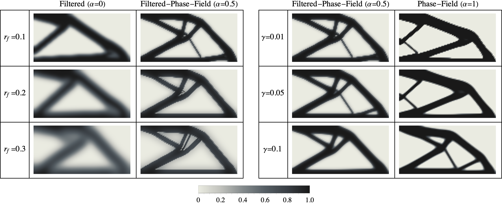
Figure 1. Cantilever beam topology optimization: optimal field $(\alpha\phi+\beta K\phi)$ obtained for $\alpha=1-\beta=0$ (F method), $\alpha=\beta=0.5$ (combined F/PF) and $\alpha=1-\beta=1$ (PF method) employing different values of the filter radius $r_{f}$ (for F and F/PF, left) and of the phase-field parameter $\gamma$ (for F/PF and PF, right). Simulation parameters (if not differently specified): $\eta=1$ N/m, $r_{f}=0.1$ m, and $\gamma=0.01$ m.

Let us firstly compare the first two columns of Figure 1, respectively corresponding to the F and the F/PF method, for different values of the filter radius $r_{f}$. The optimal phase distribution $\alpha\phi+\beta K\phi$ obtained with the F method depends on the radius $r_{f}$ of the filter. Moreover, the choice of the threshold level used to define the solid highly affects the final geometry of the structure, possibly leading to disconnections for coarse filters. The combined F/PF shows to be less influenced by the filter radius $r_{f}$, as In fact, the main geometrical features of the final topology are insensitive to the choice of this parameter. Moreover, even employing filters with large radii, grey transition regions are significantly less present in the F/PF solution than in the corresponding F solution, thus leading to a minor risk of creating disconnections when setting the threshold for the definition of the solid. Remarkably, the minimum feature sizes appearing in the final topology remain detailed and small compared to the filter radius. It is noteworthy that no post-processing technique has been employed for showing the solution fields in Figure 1. Such techniques (see, e.g., [25]) would allow to treat the issues of the F method, at the price of introducing an (undesirable) dependency of the final solution on user choices.

We now compare the last two columns of Figure 1, respectively corresponding to the F/PF and the PF method, for varying values of the user-defined parameter $\gamma$. Optimal shapes from the PF method are highly affected by the value of $\gamma$. On the contrary, final topologies from the F/PF approach seem to be much less sensitive to the different choices of the parameter. As $\gamma$ is usually fixed heuristically, we find the robustness the F/PF method with respect to this parameter particularly valuable.

In this note, we focus on the analytical aspects of method (1.5), while numerical and algorithmic considerations, as well as some simulation campaigns, will be presented in a forthcoming publication. At first, we prove that optimal shapes exist for any choice of parameters $\alpha$, $\beta$, and $\gamma$ (Theorem 2.1). This existence proof is closely reminiscent of that of [10].

We then prove that optimal shapes depend continuously (up to subsequences) on the parameters. In particular, letting $\phi_{n}$ be optimal for parameters $(\alpha_{n},\beta_{n},\gamma_{n})$, if $(\alpha_{n},\beta_{n},\gamma_{n})\to(\alpha,\beta,\gamma)$ then (up to not relabeled subsequences) we have that $\phi_{n}\to\phi$, where $\phi$ is optimal for the parameters $(\alpha,\beta,\gamma)$ (Corollary 3.2). This convergence hinges on a more general variational approximation result of $\Gamma$-convergence type (Theorem 3.1).

Problem (1.5) is space-discretized by means of a Galerkin method in Section 4. In particular, we discuss finite-dimensional approximations of (1.5) and prove the existence of approximating optimal $\phi_{h}$. The convergence, up to subsequences, of $\phi_{h}$ to solutions to (1.5) is then recovered (Theorem 4.1).

Eventually, we show in Theorem 5.1 that the stationary points of the bilevel minimization functional $\phi\mapsto C(\phi,u)+\alpha P_{\gamma}(\phi)$ under the equilibrium constraint of (1.5) can be equivalently tackled by finding stationary points of the Hu-Washizu-type Lagrangian

$$L(\phi,u,e,\sigma) =C(\phi,u)+\frac{\alpha}{2}P_{\gamma}(\phi)-\frac{1}{2}\int_{\Omega}{\mathbb{C}}(\alpha\phi+\beta K\phi)e:e\,\mathrm{d}x$$

$$\quad+\int_{\Omega}\sigma:(e-\varepsilon(u))\,\mathrm{d}x.$$

This equivalent formulation seem new in this context and allows for an efficient numerical treatment of the topology optimization problem, that is currently under investigations from the authors.

2. Existence

The focus of this section is on proving the existence of solutions to problem (1.5). We have the following.

Theorem 2.1 (Existence).

Problem (1.5) admits a solution.

Before proving the result, let us collect notation on the equilibrium problem (1.1)-(1.3). Recall that for any $\phi\in\Phi$ one can find a unique $u\in U$ such that

$$E(\alpha\phi+\beta K\phi,u)-C(\phi,u)\leq E(\alpha\phi+\beta K\phi,\widehat{u})-C(\phi,\widehat{u})\quad\forall\widehat{u}\in U$$

or, equivalently,

$$\int_{\Omega}{\mathbb{C}}(\alpha\phi+\beta K\phi)\varepsilon(u):\varepsilon(v)\,\mathrm{d}x=\int_{\Omega}\phi f\cdot v\,\mathrm{d}x+\int_{\Gamma_{\rm N}}g\cdot f\,\mathrm{d}\Gamma\quad\forall v\in U.$$ (2.1)

This allows to define a solution operator $S_{\alpha\beta}:\Phi\to U$ as $S_{\alpha\beta}(\phi)=u$.

Standard estimates for the linear elastic system and the nondegeneracy of ${\mathbb{C}}$ entail that

$$c_{0}\|\varepsilon(u)\|_{L^{2}}^{2}\leq\|f\|_{L^{2}(\Omega;{\mathbb{R}}^{3})}\|u\|_{L^{2}(\Omega;{\mathbb{R}}^{3})}+\|g\|_{L^{2}(\Gamma_{\rm N};{\mathbb{R}}^{3})}\|u\|_{L^{2}(\Gamma_{\rm N};{\mathbb{R}}^{3})}.$$

Hence, an application of the Korn inequality ensures that $u$ is bounded in $H^{1}(\Omega;{\mathbb{R}}^{3})$. In particular,

$$\|S_{\alpha\beta}(\phi)\|_{H^{1}(\Omega;{\mathbb{R}}^{3})}\leq C,$$ (2.2)

where the constant $C$ depends on $\Omega$, $c_{0}$, $\|f\|_{L^{2}(\Omega;{\mathbb{R}}^{3})}$, and $\|g\|_{L^{2}(\Gamma_{\rm N};{\mathbb{R}}^{3})}$ but is independent of $\phi$. This in turn implies that, the compliance term $C(\phi,S_{\alpha\beta}(\phi))$ is bounded, independently of $\phi\in\Phi$.

By using the solution operator $S_{\alpha\beta}$ one can equivalently reformulate problem (1.5) as

$$\min_{\phi\in\Phi}\big{\{}C(\phi,S_{\alpha\beta}(\phi))+\alpha P_{\gamma}(\phi)\big{\}}.$$

Proof of Theorem 2.1.

Let $\phi_{n}$ be a minimizing sequence for $\phi\mapsto C(\phi,S_{\alpha\beta}(\phi))+\alpha P_{\gamma}(\phi)$ and let $u_{n}=S_{\alpha\beta}(\phi_{n})$. As $\phi_{n}\in[0,1]$ almost everywhere and $u_{n}$ is bounded in $H^{1}(\Omega;{\mathbb{R}}^{3})$ by (2.2), by passing to some not relabeled subsequence we have that $\phi_{n}\stackrel{{\scriptstyle\ast}}{{\rightharpoonup}}\phi$ in $L^{\infty}(\Omega)$ and $u_{n}\rightharpoonup u$ in $H^{1}(\Omega;{\mathbb{R}}^{3})$. By compactness we also have that $u_{n}\to u$ in $L^{6-}(\Omega;{\mathbb{R}}^{3})$. In particular, we have that $f\cdot u_{n}\to f\cdot u$ in $L^{3/2-}(\Omega)$ and we can conclude that

$$C(\phi_{n},u_{n})\to C(\phi,u).$$ (2.3)

We now proceed by considering separately the cases $\alpha>0$ and $\alpha=0$.

Case $\alpha>0$: The boundedness of $C(\phi_{n},S_{\alpha\beta}(\phi_{n}))+\alpha P_{\gamma}(\phi_{n})$ and the fact that $C(\phi_{n},S_{\alpha\beta}(\phi_{n}))$ is bounded entail that $\phi_{n}$ is bounded in $H^{1}(\Omega)$ (if $\gamma>0$) or $BV(\Omega)$ (if $\gamma=0$). In both cases, $\phi_{n}$ is precompact in $L^{1}(\Omega)$ so that one can assume with no loss of generality (or extract again, without relabeling) that $\phi_{n}\to\phi$ in $L^{1}(\Omega)$ as well. Hence, $\alpha\phi_{n}+\beta K\phi_{n}\to\alpha\phi+\beta K\phi$ in $L^{1}(\Omega)$, independently of the value of $\beta\geq 0$. Due to the Lipschitz continuity and the boundedness of ${\mathbb{C}}$ we hence have that

$${\mathbb{C}}(\alpha\phi_{n}+\beta K\phi_{n})\to{\mathbb{C}}(\alpha\phi+\beta K\phi)\quad\text{in}\ L^{q}(\Omega;{\mathbb{R}}^{3\times 3\times 3\times 3}),\ \forall q\in[1,\infty).$$ (2.4)

Since ${\mathbb{C}}$ is uniformly positive, we equivalently have that ${\mathbb{C}}(\alpha\phi_{n}+\beta K\phi_{n})^{1/2}\to{\mathbb{C}}(\alpha\phi+\beta K\phi)^{1/2}$ in $L^{q}(\Omega;{\mathbb{R}}^{3\times 3\times 3\times 3})$ for all $q\in[1,\infty)$, where the superscript ${1/2}$ denotes the square-root tensor. This convergence, as well as the boundedness of ${\mathbb{C}}$, allows us to conclude that

$${\mathbb{C}}(\alpha\phi_{n}+\beta K\phi_{n})^{1/2}\varepsilon(u_{n})\rightharpoonup{\mathbb{C}}(\alpha\phi+\beta K\phi)^{1/2}\varepsilon(u)\quad\text{in}\ L^{2}(\Omega;{\mathbb{R}}^{3\times 3}).$$ (2.5)

Let now $u^{*}\in U$ and choose $u_{m}^{*}\in U\cap W^{1,\infty}(\Omega,{\mathbb{R}}^{3})$ with $u_{m}^{*}\to u^{*}$ in $H^{1}(\Omega;{\mathbb{R}}^{3})$. Making use of (2.4)-(2.8) we obtain

$$E(\alpha\phi+\beta K\phi,u)-C(\phi,u)\leq\liminf_{n\to\infty}\Big{(}E(\alpha\phi_{n}+\beta K\phi_{n},u_{n})-C(\phi_{n},u_{n})\Big{)}$$

$$\quad\leq\liminf_{n\to\infty}\Big{(}E(\alpha\phi_{n}+\beta K\phi_{n},u_{m}^{*})-C(\phi_{n},u_{m}^{*})\Big{)}$$

$$\quad=E(\alpha\phi+\beta K\phi,u_{m}^{*})-C(\phi,u_{m}^{*}).$$ (2.6)

Passing to the limit for $m\to\infty$, we have proved that $u=S_{\alpha\beta}(\phi)$.

Recall that we have that $\phi_{n}\to\phi$ in $L^{1}(\Omega)$. Moreover, since $\phi_{n}\in[0,1]$ a.e., this entails that $\phi_{n}\to\phi$ in $L^{q}(\Omega)$ for all $q\in[1,\infty)$. In particular, if $\gamma>0$ one can pass the term $\int_{\Omega}\phi_{n}^{2}(1-\phi_{n})^{2}\,\mathrm{d}x$ to the limit and check that $P_{\gamma}(\phi)\leq\liminf P_{\gamma}(\phi_{n})$. If $\gamma=0$ one uses the lower semicontinuity if the perimeter in $BV$ to get $P_{0}(\phi)\leq\liminf P_{0}(\phi_{n})$. As we have already checked that $C(\phi_{n},u_{n})\to C(\phi,u)$ we conclude that

$$C(\phi,u)+\alpha P_{\gamma}(\phi)\leq\liminf_{n\to\infty}\Big{(}C(\phi_{n},u_{n})+\alpha P_{\gamma}(\phi_{n})\Big{)}$$

for all $\gamma\geq 0$ and $\phi$ is a solution of problem (1.5).

Case $\alpha=0$: As $\phi_{n}\stackrel{{\scriptstyle\ast}}{{\rightharpoonup}}\phi$ in $L^{\infty}(\Omega)$ and $K:L^{\infty}(\Omega)\to L^{1}(\Omega)$ is compact, we have that $\beta K\phi_{n}\to\beta K\phi$ in $L^{1}(\Omega)$, independently of the value of $\beta\geq 0$. Arguing as in (2.4) we have

$${\mathbb{C}}(\beta K\phi_{n})^{1/2}\to{\mathbb{C}}(\beta K\phi)^{1/2}\ \ \text{in}\ \ L^{q}(\Omega;{\mathbb{R}}^{3\times 3\times 3\times 3}),\ \forall q\in[1,\infty).$$ (2.7)

This entails that

$${\mathbb{C}}(\beta K\phi_{n})^{1/2}\varepsilon(u_{n})\rightharpoonup{\mathbb{C}}(\beta K\phi)^{1/2}\varepsilon(u)\quad\text{in}\ L^{2}(\Omega;{\mathbb{R}}^{3\times 3}).$$ (2.8)

Repeating the argument in (2.6) for $\alpha=0$ we get

$$E(\beta K\phi,u)-C(\phi,u)\leq E(\beta K\phi,u^{*})-C(\phi,u^{*})\quad\forall u^{*}\in U$$

so that $u=S_{0\beta}(\phi)$. As (2.3) holds, this concludes the proof that $\phi$ is a solution of problem (1.5). ∎

3. $\Gamma$-convergence and parameter asymptotics

In this section, we provide asymptotic results in relation with limits in the parameters. We argue within the classical frame of $\Gamma$-convergence [16]. To this aim, it is notationally advantageous to incorporate constraints into the definitions of the functionals by letting $G_{\alpha\beta\gamma}:L^{\infty}(\Omega)\times U\to(-\infty,\infty]$ be defined as

$$G_{\alpha\beta\gamma}(\phi,u)=\left\{\begin{array}[]{ll}C(\phi,u)+\alpha P_{\gamma}(\phi)&\quad\text{if}\ \phi\in\Phi\ \text{and}\ u=S_{\alpha\beta}(\phi)\\ \infty&\quad\text{otherwise}.\end{array}\right.$$

Our $\Gamma$-convergence result reads as follows.

Theorem 3.1 ($\Gamma$-convergence).

Let $(\alpha_{n},\beta_{n},\gamma_{n})\to(\alpha,\beta,\gamma)$ with $\alpha>0$ or $\beta>0$. Then, $G_{\alpha_{n}\beta_{n}\gamma_{n}}\to G_{\alpha\beta\gamma}$ in the sense of $\Gamma$-convergence with respect to the weak$\ast$ topology of $L^{\infty}(\Omega)\times U$.

Proof.

In order to prove the $\Gamma$-convergence $G_{\alpha_{n}\beta_{n}\gamma_{n}}\to G_{\alpha\beta\gamma}$ we check below the corresponding $\liminf$-inequality and we exhibit recovery sequences [16].

Liminf-inequality. Let $(\phi_{n},u_{n})$ be given in such a way that $(\phi_{n},u_{n})\stackrel{{\scriptstyle\ast}}{{\rightharpoonup}}(\phi,u)$ in $L^{\infty}(\Omega)\times U$ and assume with no loss of generality that

$$\sup_{n\in\mathbb{N}}G_{\alpha_{n}\beta_{n}\gamma_{n}}(\phi_{n},u_{n})<\infty.$$ (3.1)

In particular, $\phi_{n}\in\Phi$ and $u_{n}=S_{\alpha_{n}\beta_{n}}(\phi_{n})$ for all $n$, and, by possibly extracting without relabeling, we can assume that $u_{n}\to u$ in $L^{6-}(\Omega;{\mathbb{R}}^{3})$.

Let us now proceed by distinguishing cases.

Case $\alpha>0$ and $\gamma>0$: We have that $\phi_{n}$ are weakly precompact in $H^{1}(\Omega)$, hence strongly precompact in $L^{1}(\Omega)$. This entails that

$$\alpha_{n}\phi_{n}+\beta_{n}K\phi_{n}\to\alpha\phi+\beta K\phi\quad\text{in}\ L^{1}(\Omega)$$ (3.2)

along a not relabeled subsequence, independently of the value of $\beta\geq 0$. Moving from (3.2), the proof of Theorem 2.1 can be replicated verbatim, concluding that $u=S_{\alpha\beta}(\phi)$.

In order to establish the $\Gamma$-$\liminf$ inequality $G_{\alpha\beta\gamma}(\phi,u)\leq\liminf G_{\alpha_{n}\beta_{n}\gamma_{n}}(\phi_{n},u_{n})$ we just need to show that

$$C(\phi,u)+\alpha P_{\gamma}(\phi)\leq\liminf_{n\to\infty}\Big{(}C(\phi_{n},u_{n})+\alpha_{n}P_{\gamma_{n}}(\phi_{n})\Big{)}.$$ (3.3)

By following again the proof of Theorem 2.1, we obtain that $C(\phi_{n},u_{n})\to C(\phi,u)$. One can assume with no loss of generality that $\alpha_{n}\geq\alpha/2$ and $\gamma_{n}\geq\gamma/2>0$ for all $n$, so that, possibly extracting without relabeling, bound (3.1) entails that $\phi_{n}\rightharpoonup\phi$ in $H^{1}(\Omega)$. Hence, $P_{\gamma}(\phi)\leq\liminf P_{\gamma_{n}}(\phi_{n})$ and we have that (3.3) holds.

Case $\alpha>0$ and $\gamma=0$: We proceed as before in order to check that $u=S_{\alpha\beta}(\phi)$. Inequality (3.3) follows now by the classical Modica-Mortola result [22], yielding $P_{0}(\phi)\leq\liminf P_{\gamma_{n}}(\phi_{n})$.

Case $\alpha=0$: the compactness of $K$ suffices to conclude for

$$\alpha_{n}\phi_{n}+\beta_{n}K\phi_{n}\to\beta K\phi\quad\text{in}\ L^{1}(\Omega)$$ (3.4)

independently of the value of $\beta\geq 0$. This again ensures that $u=S_{0\beta}(\phi)$.

The argument of Theorem 2.1 entails that $C(\phi_{n},u_{n})\to C(\phi,u)$ and the $\Gamma$-$\liminf$ inequality

$$G_{0\beta\gamma}(\phi,u)=C(\phi,u)=\lim_{n\to\infty}C(\phi_{n},u_{n})$$

$$\quad\leq\liminf_{n\to\infty}\Big{(}C(\phi_{n},u_{n})+\alpha_{n}P_{\gamma_{n}}(\phi_{n})\Big{)}=\liminf_{n\to\infty}G_{\alpha_{n}\beta_{n}\gamma_{n}}(\phi_{n},u_{n})$$

trivially follows, independently of the values of $\beta\geq 0$ and $\gamma\geq 0$.

Recovery sequence. Let $(\phi^{*},u^{*})\in L^{\infty}(\Omega)\times U$ with $G_{\alpha\beta\gamma}(\phi^{*},u^{*})<\infty$ be given. We aim at finding a recovery sequence $(\phi_{n}^{*},u_{n}^{*})\stackrel{{\scriptstyle\ast}}{{\rightharpoonup}}(\phi^{*},u^{*})$ in $L^{\infty}(\Omega)\times U$ (at least) such that $G_{\alpha_{n}\beta_{n}\gamma_{n}}(\phi_{n}^{*},u_{n}^{*})\to G_{\alpha\beta\gamma}(\phi^{*},u^{*})$.

We distinguish here the two cases: $\gamma>0$ and $\gamma=0$.

Case $\gamma>0$: Independently of the values $\alpha,\,\beta\geq 0$, we simply exploit pointwise convergence and define $\phi_{n}^{*}=\phi^{*}$ and $u_{n}^{*}=S_{\alpha_{n}\beta_{n}}(\phi^{*})$. As $\alpha_{n}\phi^{*}+\beta_{n}K\phi^{*}\to\alpha\phi^{*}+\beta K\phi^{*}$ in $L^{1}(\Omega)$, it is standard to check that $u_{n}^{*}\rightharpoonup u^{*}$ in $H^{1}(\Omega;{\mathbb{R}}^{3})$, so that one has

$$C(\phi_{n}^{*},u_{n}^{*})+\alpha_{n}P_{\gamma_{n}}(\phi_{n}^{*})=C(\phi^{*},u_{n}^{*})+\alpha_{n}P_{\gamma_{n}}(\phi^{*})\to C(\phi^{*},u^{*})+\alpha F_{\gamma}(\phi^{*})$$

and the convergence $G_{\alpha_{n}\beta_{n}\gamma_{n}}(\phi_{n}^{*},u_{n}^{*})\to G_{\alpha\beta\gamma}(\phi^{*},u^{*})$ follows.

Case $\gamma=0$: For all $\alpha,\,\beta\geq 0$, we resort again to the classical Modica-Mortola construction [22] in order to find $\phi_{n}^{*}\to\phi^{*}$ such that $P_{\gamma_{n}}(\phi_{n}^{*})\to P_{0}y(\phi^{*})$. Correspondingly, we define again $u_{n}^{*}=S_{\alpha_{n}\beta_{n}}(\phi_{n}^{*})$. As one again has that $\alpha_{n}\phi_{n}^{*}+\beta_{n}K\phi_{n}^{*}\to\alpha\phi^{*}+\beta K\phi^{*}$ in $L^{1}(\Omega)$, one can still conclude that $u_{n}^{*}\rightharpoonup u^{*}$ in $H^{1}(\Omega;{\mathbb{R}}^{3})$. Hence, convergence

$$C(\phi_{n}^{*},u_{n}^{*})+\alpha_{n}P_{\gamma_{n}}(\phi_{n}^{*})\to C(\phi^{*},u^{*})+\alpha F_{0}(\phi^{*})$$

holds and $G_{\alpha_{n}\beta_{n}\gamma_{n}}(\phi_{n}^{*},u_{n}^{*})\to G_{\alpha\beta 0}(\phi^{*},u^{*})$ follows. ∎

The bound (2.2) readily entails that the functionals $G_{\alpha\beta\gamma}$ are equicoercive with respect to the weak$\ast$ topology in $L^{\infty}(\Omega)\times U$. The following is hence a straightforward consequence of Theorem 3.1.

Corollary 3.2 (Parameter asymptotics).

Let $\phi_{\alpha_{n}\beta_{n}\gamma_{n}}$ solve problem (1.5) with parameters $(\alpha_{n},\beta_{n},\gamma_{n})$. Moreover, let $(\alpha_{n},\beta_{n},\gamma_{n})\to(\alpha,\beta,\gamma)$. Then, $\phi_{\alpha_{n}\beta_{n}\gamma_{n}}\stackrel{{\scriptstyle\ast}}{{\rightharpoonup}}\phi_{\alpha\beta\gamma}$ in $L^{\infty}(\Omega)$ up to a not relabeled subsequence, where $\phi_{\alpha\beta\gamma}$ solves (1.5) with parameters $(\alpha,\beta,\gamma)$. If $\alpha>0$ then $\phi_{\alpha_{n}\beta_{n}\gamma_{n}}$ converges also strongly in $L^{q}(\Omega)$ for all $q\in[1,\infty)$. Moroever, it converges weakly in $H^{1}(\Omega)$ if $\gamma>0$, and weakly$\ast$ in $BV(\Omega)$ if $\gamma=0$.

4. Space discretization

We describe now a space-discretization procedure via a Galerkin method. Although our approach is abstract, assumptions are modeled on the case of conformal finite elements. Let $\Phi_{h}\subset\Phi$ and $U_{h}\subset U$ be two families of finite-dimensional subspaces with $\Phi_{h}\subset\Phi_{h^{\prime}}$ and $U_{h}\subset U_{h^{\prime}}$ for $h^{\prime}\leq h$, $\cup_{h}\Phi_{h}$ dense in $\Phi$, and $\cup_{h}U_{h}$ dense in $U$. We also assume that $\cup_{h}U_{h}$ is dense in $W^{1,\infty}(\Omega;{\mathbb{R}}^{3})$ with respect to its topology. These assumptions are fulfilled by choosing $\Phi_{h}$ and $U_{h}$ as spaces of piecewise polynomials of degree $0$ and $1$ on a given regular triangulation of $\Omega$ (assume it to be a polygon) with mesh size $h>0$.

For the sake of simplicity, we assume to be able to evaluate the functionals $E$, $P_{\gamma}$, and $C$ exactly on $\Phi_{h}$ and $U_{h}$. Note however that the analysis can be extended to the case of approximating $E_{h}$, $F_{\gamma h}$, and $C_{h}$ at the expense of some additional notational intricacy only, see [18, Sec. IV.27.4.2], as well as the classical references [14, 26]. On the contrary, we assume to be given a family of linear and continuous operators $K_{h}:\Phi_{h}\to\Phi_{h}$ fulfilling the continuous convergence requirement

$$\phi_{h}\stackrel{{\scriptstyle\ast}}{{\rightharpoonup}}\phi\ \ \text{in}\ L^{\infty}(\Omega)\quad\Rightarrow\quad K_{h}\phi_{h}\to K\phi\ \ \text{in}\ L^{1}(\Omega).$$ (4.1)

The latter can be readily met in practice, if $K$ is chosen to have form (1.6).

The space-discrete version of problem (1.5) reads as follows

$$\min_{\phi_{h}\in\Phi_{h}}\bigg{\{}C(\phi_{h},u_{h})+\alpha P_{\gamma}(\phi_{h}):$$

$$\quad u_{h}=\operatorname*{arg\,min}_{v_{h}\in U_{h}}\big{(}E(\alpha\phi_{h}+\beta K_{h}\phi_{h},v_{h})-C(\phi_{h},v_{h})\big{)}\bigg{\}}$$ (4.2)

Note that the latter makes sense, for $v_{h}\mapsto E(\alpha\phi_{h}+\beta K_{h}\phi_{h},v_{h})-C(\phi_{h},v_{h})$ admits a unique minimizer in $U_{h}$ for all $\phi_{h}\in\Phi_{h}$ due to the Lax-Milgram Lemma. In particular, this defines the discrete solution operator $S_{\alpha\beta h}:\Phi_{h}\to U_{h}$ as $u_{h}=S_{\alpha\beta h}(\phi_{h})$, allowing to equivalently rewrite problem (4.2) as follows

$$\min_{\phi_{h}\in\Phi_{h}}\big{\{}C(\phi_{h},S_{\alpha\beta h}(\phi_{h}))+\alpha P_{\gamma}(\phi_{h})\big{\}}.$$ (4.3)

The main result of this section is the following.

Theorem 4.1 (Space discretization).

For all $h>0$ problem (4.3) admits a solution $\phi_{h}$. There exists a positive constant $C$ depending on $c_{0}$, $\Omega$, $\|f\|_{L^{2}(\Omega;{\mathbb{R}}^{3})}$, and $\|g\|_{L^{2}(\Gamma_{\rm N};{\mathbb{R}}^{3})}$ but independent of $h$, $\alpha$, and $\beta$ such that $\|u_{h}\|_{H^{1}(\Omega;{\mathbb{R}}^{3})}\leq C$, for $u_{h}=S_{\alpha\beta h}(\phi_{h})$. As $h\to 0$, one can find not relabeled subsequences such that $\phi_{h}\stackrel{{\scriptstyle\ast}}{{\rightharpoonup}}\phi$ in $L^{\infty}(\Omega)$ and $u_{h}\rightharpoonup u$ in $H^{1}(\Omega;{\mathbb{R}}^{3})$, where $\phi$ solves the limiting problem (1.5) and $u=S_{\alpha\beta}(\phi)$. If $\alpha>0$ then $\phi_{h}$ converges also strongly in $L^{q}(\Omega)$ for all $q\in[1,\infty)$, weakly in $H^{1}(\Omega)$ if $\gamma>0$, and weakly$\ast$ in $BV(\Omega)$ if $\gamma=0$.

Proof.

The existence of space-discrete solutions $\phi_{h}$ follows by the same argument as in Theorem 2.1. The situation is even simpler here, for the finite dimensionality of the problem entails that, for $h$ fixed, a minimizing sequence $\phi_{hn}$ for (4.3) is strongly compact in $L^{\infty}(\Omega)$ (and, for $\alpha>0$, in $H^{1}(\Omega)$ or $BV(\Omega)$, depending on $\gamma$).

Let now $\phi_{h}$ solve (4.3) and $u_{h}=S_{\alpha\beta h}(\phi_{h})$. The bound on $\|u_{h}\|_{H^{1}(\Omega;{\mathbb{R}}^{3})}$ can be obtained as in (2.2). As $\phi_{h}\in[0,1]$ a.e., as $h\to 0$ one can extract (without relabelling) and have $\phi_{h}\stackrel{{\scriptstyle\ast}}{{\rightharpoonup}}\phi$ in $L^{\infty}(\Omega)$ and $u_{h}\rightharpoonup u$ in $H^{1}(\Omega;{\mathbb{R}}^{3})$. Moreover, the above bounds ensure that $C(\phi_{h},u_{h})$ is bounded, independently of $h$. Hence, if $\alpha>0$ one can assume that $\phi_{h}$ converges also strongly in $L^{q}(\Omega)$ for all $q\in[1,\infty)$, weakly in $H^{1}(\Omega)$ if $\gamma>0$, and weakly$\ast$ in $BV(\Omega)$ if $\gamma=0$.

In all cases, by using the continuous-convergence assumption (4.1) we have that $\alpha\phi_{h}+\beta K_{h}\phi_{h}\to\alpha\phi+\beta K\phi$ in $L^{1}(\Omega)$. By following the argument of Theorem 2.1, we again obtain that

$${\mathbb{C}}(\alpha\phi_{h}+\beta K_{h}\phi_{h})\to{\mathbb{C}}(\alpha\phi+\beta K\phi)\quad\text{in}\ L^{q}(\Omega;{\mathbb{R}}^{3\times 3\times 3\times 3})\quad\forall q\in[1,\infty),$$ (4.4)

$${\mathbb{C}}(\alpha\phi_{h}+\beta K_{h}\phi_{h})^{1/2}\varepsilon(u_{h})\rightharpoonup{\mathbb{C}}(\alpha\phi+\beta K\phi)^{1/2}\varepsilon(u)\quad\text{in}\ L^{2}(\Omega;{\mathbb{R}}^{3\times 3}).$$ (4.5)

Let now $v_{m}\in W^{1,\infty}(\Omega;{\mathbb{R}}^{3})$ be given and approximate it via $v_{h}\in U_{h}$ such that $v_{h}\to v_{m}$ in $W^{1,\infty}(\Omega;{\mathbb{R}}^{3})$ as $h\to 0$. Using the convergences (4.4)-(4.5) and the fact that $C(\phi_{h},u_{h})\to C(\phi,u)$ we deduce that

$$E(\alpha\phi+\beta K\phi,u)-C(\phi,u)\leq\liminf_{h\to 0}\Big{(}E(\alpha\phi_{h}+\beta K_{h}\phi_{h},u_{h})-C(\phi_{h},u_{h})\Big{)}$$

$$\quad\leq\liminf_{h\to 0}\Big{(}E(\alpha\phi_{h}+\beta K_{h}\phi_{h},v_{h})-C(\phi_{h},v_{h})\Big{)}=E(\alpha\phi+\beta K\phi,v_{m})-C(\phi,v_{m}).$$

Eventually, for all $v\in U$ one can find a sequence $v_{m}\in W^{1,\infty}(\Omega;{\mathbb{R}}^{3})$ such that $v_{m}\to v$ in $H^{1}(\Omega;{\mathbb{R}}^{3})$ as $m\to\infty$. By passing to the limit as $m\to\infty$ in the above inequality ensures that $u\in S_{\alpha\beta}(\phi)$.

The last step of the proof consists in remarking that

$$C(\phi,u)+\alpha P_{\gamma}(\phi)\leq\liminf_{h\to 0}\Big{(}C(\phi_{h},u_{h})+\alpha P_{\gamma}(\phi_{h})\Big{)}$$

independently of the values of the parameters $(\alpha,\beta,\gamma)$. In fact, one has that $\color[rgb]{0,0,0}\alpha\color[rgb]{0,0,0}P_{\gamma}(\phi)\leq\liminf_{h\to 0}\alpha P_{\gamma}(\phi_{h})$, for any $\alpha\geq 0$. Eventually, we have checked that $\phi$ solves (4.3). ∎

Before closing this section, let us remark that the above analysis can be extended to include parameter asymptotics, in the same spirit of Section 3.

5. Lagrangian formulation

The actual implementation of the bilevel minimization of problem (1.5) is computationally demanding. On the contrary, stationary points of the bilevel minimization functional $\phi\mapsto C(\phi,S_{\alpha\beta}(\phi))+\alpha P_{\gamma}(\phi)$ can be efficiently tackled by equivalently reformulating the problem in terms of stationarity of the Lagrangian $L:\Phi\times U\times L^{2}(\Omega;{\mathbb{R}}^{3\times 3})\times L^{2}(\Omega;{\mathbb{R}}^{3\times 3})\to{\mathbb{R}}$ given by

$$L(\phi,u,e,\sigma) =C(\phi,u)+\frac{\alpha}{2}P_{\gamma}(\phi)-\frac{1}{2}\int_{\Omega}{\mathbb{C}}(\alpha\phi+\beta K\phi)e:e\,\mathrm{d}x$$

$$\quad+\int_{\Omega}\sigma:(e-\varepsilon(u))\,\mathrm{d}x.$$

The fact that stationary points of $\phi\mapsto C(\phi,S_{\alpha\beta}(\phi))+\alpha P_{\gamma}(\phi)$ and (the first component of) stationary points of the Lagrangian $L$ coincide was already used without proof in [21] in the setting of the PF method ($\alpha=1$, $\beta=0$). On the other hand, such monolithic formulation seems to be new in the frame of the F method ($\alpha=0$, $\beta=1$).

Note that, for the purposes of simplifying the presentation, the constraints $\phi\in[0,1]$ and $\int_{\Omega}\phi\,\mathrm{d}x=v_{0}$ are neglected throughout this section. Our main result is the following.

Theorem 5.1 (Lagrangian formulation).

$\phi$ is a stationary point of $C(\phi,S_{\alpha\beta}(\phi))+\alpha P_{\gamma}(\phi)$ if and only if the Lagrangian $L$ is stationary at $(\phi,S_{\alpha\beta}(\phi),\varepsilon(S_{\alpha\beta}(\phi)),{\mathbb{C}}(\alpha\phi+\beta K\phi)\varepsilon(S_{\alpha\beta}(\phi)))$.

Proof.

By computing variations of (2.1) for $u=S_{\alpha\beta}(\phi)$ in direction $\tilde{\phi}\in L^{\infty}(\Omega)$ (in the case with constraints we would require $\int_{\Omega}\tilde{\phi}\,\mathrm{d}x=0$ and $\phi+t\tilde{\phi}\in[0,1]$ a.e., for $t$ small enough), we get that

$$\int_{\Omega}{\mathbb{C}}(\alpha\phi+\beta K\phi)\varepsilon(DS_{\alpha\beta}(\phi)[\tilde{\phi}]):\varepsilon(v)\,\mathrm{d}x$$

$$\qquad+\int_{\Omega}D{\mathbb{C}}(\alpha\phi+\beta K\phi)[\alpha\tilde{\phi}+\beta K\tilde{\phi}]\varepsilon(S_{\alpha\beta}(\phi)):\varepsilon(v)\,\mathrm{d}x$$

$$\quad=\int_{\Omega}\tilde{\phi}f\cdot v\,\mathrm{d}x\quad\forall v\in U.$$ (5.1)

Here, $DS_{\alpha\beta}(\phi)[\tilde{\phi}]\in U$ and $D{\mathbb{C}}(\alpha\phi+\beta K\phi)[\alpha\tilde{\phi}+\beta K\tilde{\phi}]$ are the Gateaux derivatives of $\phi\mapsto S_{\alpha\beta}(\phi)$ and $\phi\mapsto{\mathbb{C}}(\alpha\phi+\beta K\phi)$ at $\phi$ in direction $\tilde{\phi}$, respectively.

Compute now the variations of $L$ at $(\phi,u,e,\sigma)$ in directions $(\tilde{\phi},\tilde{u},\tilde{e},\tilde{\sigma})$ and get

$$\delta_{\phi}L(\phi,u,e,\sigma)[\tilde{\phi},\tilde{u},\tilde{e},\tilde{\sigma}] =\int_{\Omega}\tilde{\phi}f\cdot u\,\mathrm{d}x+\frac{\alpha}{2}\delta P_{\gamma}(\phi)[\tilde{\phi}]$$

$$\quad-\frac{1}{2}\int_{\Omega}D{\mathbb{C}}(\alpha\phi+\beta K\phi)[\alpha\tilde{\phi}+\beta K\tilde{\phi}]e:e\,\mathrm{d}x,$$

$$\delta_{u}L(\phi,u,e,\sigma)[\tilde{\phi},\tilde{u},\tilde{e},\tilde{\sigma}] =\int_{\Omega}\phi f\cdot\tilde{u}\,\mathrm{d}x+\int_{\Gamma_{\rm N}}g\cdot\tilde{u}\,\mathrm{d}\Gamma+\int_{\Omega}\sigma:\varepsilon(\tilde{u}),$$

$$\delta_{e}L(\phi,u,e,\sigma)[\tilde{\phi},\tilde{u},\tilde{e},\tilde{\sigma}] =-\int_{\Omega}\big{(}{\mathbb{C}}(\alpha\phi+\beta K\phi)e-\sigma\big{)}:\tilde{e}\,\mathrm{d}x,$$

$$\delta_{\sigma}L(\phi,u,e,\sigma)[\tilde{\phi},\tilde{u},\tilde{e},\tilde{\sigma}] =\int_{\Omega}\tilde{\sigma}:(e-\varepsilon(u))\,\mathrm{d}x.$$

Note that

$$\delta_{e}L(\phi,u,e,\sigma)=0\quad \Leftrightarrow\quad\sigma={\mathbb{C}}(\alpha\phi+\beta K\phi)e\quad\text{a.e.},$$

$$\delta_{\sigma}L(\phi,u,e,\sigma)=0\quad \Leftrightarrow\quad e=\varepsilon(u)\quad\text{a.e}.$$

Indeed, stationarity in $e$ and $\sigma$ deliver the constitutive equation and the kinematic compatibility, respectively. On the other hand, stationarity in $u$ corresponds to equilibrium. In particular, $u=S_{\alpha\beta}(\phi)$ turns out to be equivalent to $\delta_{u}L=0$, $\delta_{e}L=0$, and $\delta_{\sigma}L=0$ at the point $(\phi,u,e,\sigma)=(\phi,S_{\alpha\beta}(\phi),\varepsilon(S_{\alpha\beta}(\phi)),{\mathbb{C}}(\alpha\phi+\beta K\phi)\varepsilon(S_{\alpha\beta}(\phi)))$.

In order to conclude the proof, we compute the variation of $\phi\mapsto C(\phi,S_{\alpha\beta}(\phi))+\alpha P_{\gamma}(\phi)$ in direction $\tilde{\phi}$ getting

$$\delta\big{(}C(\phi,S_{\alpha\beta}(\phi))+\alpha P_{\gamma}(\phi)\big{)}[\tilde{\phi}]=\int_{\Omega}\tilde{\phi}f\cdot S_{\alpha\beta}(\phi)\,\mathrm{d}x+\int_{\Omega}\phi f\cdot DS_{\alpha\beta}(\phi)[\tilde{\phi}]\,\mathrm{d}x$$

$$\quad+\int_{\Gamma_{\rm N}}g\cdot DS_{\alpha\beta}(\phi)[\tilde{\phi}]\,\mathrm{d}\Gamma+\alpha\delta P_{\gamma}(\phi)[\tilde{\phi}].$$

By using relation (5.1) and setting $u=S_{\alpha\beta}(\phi)$ we obtain that

$$\delta\big{(}C(\phi,S_{\alpha\beta}(\phi))+\alpha P_{\gamma}(\phi)\big{)}[\tilde{\phi}]$$

$$\quad=\int_{\Omega}\tilde{\phi}f\cdot S_{\alpha\beta}(\phi)\,\mathrm{d}x+\int_{\Omega}{\mathbb{C}}(\alpha\phi+\beta K\phi)\varepsilon(DS_{\alpha\beta}(\phi)[\tilde{\phi}]):\varepsilon(u)\,\mathrm{d}x+\alpha\delta P_{\gamma}(\phi)[\tilde{\phi}]$$

$$\quad=2\int_{\Omega}\tilde{\phi}f\cdot S_{\alpha\beta}(\phi)\,\mathrm{d}x-\int_{\Omega}D{\mathbb{C}}(\alpha\phi+\beta K\phi)[\alpha\tilde{\phi}+\beta K\tilde{\phi}]\varepsilon(u):\varepsilon(u)\,\mathrm{d}x$$

$$\qquad+\alpha\delta P_{\gamma}(\phi)[\tilde{\phi}]$$

$$\quad=2\delta_{\phi}L(\phi,u,e,\sigma)[\tilde{\phi},\tilde{u},\tilde{e},\tilde{\sigma}]$$

and the assertion follows. ∎

References

• [1] G. Allaire. Shape optimization by the homogenization method. Applied Mathematical Sciences, 146. Springer-Verlag, New York, 2002.
• [2] S. Almi, U. Stefanelli. Topology optimization for incremental elastoplasticity: a phase-field approach. SIAM J. Control Optim. 59 (2021), no. 1, 339–364.
• [3] S. Almi, U. Stefanelli. Topology optimization for quasistatic elastoplasticity. ESAIM Control Optim. Calc. Var. 28 (2022), art. 47.
• [4] O. Amir, B. S. Lazarov. Achieving stress-constrained topological design via length scale control. Struct. Multidiscip. Optim. 58 (2018), no. 5, 2053–2071.
• [5] F. Auricchio, E. Bonetti, M. Carraturo, D. Hömberg,A. Reali, E. Rocca. A phase-field-based graded-material topology optimization with stress constraint. Math. Models Methods Appl. Sci. 30 (2020), no. 8, 1461–1483.
• [6] M. P. Bendsøe, N. Kikuchi. Generating optimal topologies in strutural design using a homogenization method. Comput. Methods Appl. Mech. Engrg. 71 (1988), 2:197–224.
• [7] M. P. Bendsøe, O. Sigmund. Topology optimization. Theory, methods and appliations. Springer-Verlag, Berlin, 2003.
• [8] L. Blank, M. H. Farshbaf-Shaker, H. Garcke, V. Styles. Relating phase field and sharp interface approaches to structural topology optimization. ESAIM Control Optim. Calc. Var. 20 (2014), 4:1025–1058.
• [9] T.  Borrvall, J. Petersson. Topology optimization using regularized intermediate density control. Comput. Methods Appl. Mech. Engrg. 190 (2001), no. 37–38, 4911–4928.
• [10] B. Bourdin. Filters in topology optimization. Internat. J. Numer. Methods Engrg. 50 (2001), no. 9, 2143–2158.
• [11] B. Bourdin, A. Chambolle. Design-dependent loads in topology optimization. ESAIM Control Optim. Calc. Var. 9 (2003), 19–48.
• [12] T. E.  Bruns, D. A. Tortorelli. Topology optimization of geometrically nonlinear structures and compliant mechanisms. Proceedings 7th AIAA/USAF/NASA/ISSMO Symposium on Multidisciplinary Analysis and Optimization, St. Louis, MI, 2–4 September 1998; 1874–1882.
• [13] M. Burger, R. Stainko. Phase-field relaxation of topology optimization with local stress constraints. SIAM J. Control Optim. 45 (2006), no. 4, 1447–1466.
• [14] P. G. Ciarlet. The finite element method for elliptic problems. Studies in Mathematics and its Applications, Vol. 4. North-Holland Publishing Co., Amsterdam-New York-Oxford, 1978.
• [15] A. Clausen, E. Andreassen. On filter boundary conditions in topology optimization. Struct. Multidiscip. Optim. 56 (2017), no. 5, 1147–1155.
• [16] G. Dal Maso. An introduction to $\Gamma$-convergence. Progress in Nonlinear Differential Equations and their Applications, 8. Birkhäuser Boston Inc., Boston, MA, 1993.
• [17] L. Dedè, M. J. Borden, T. J. R. Hughes. Isogeometric analysis for topology optimization with a phase field model. Arch. Comput. Methods Eng. 19 (2012), no. 3, 427–465.
• [18] A. Ern, J.-L. Guermond. Finite elements II – Galerkin approximation, elliptic and mixed PDEs. Texts in Applied Mathematics, 73. Springer, Cham, 2021.
• [19] H. Garcke, P. Hüttl, P. Knopf. Shape and topology optimization involving the eigenvalues of an elastic structure: a multi-phase-field approach. Adv. Nonlinear Anal. 11 (2022), no. 1, 159–197.
• [20] B. S. Lazarov, O. Sigmund. Filters in topology optimization based on Helmholtz-type differential equations. Internat. J. Numer. Methods Engrg. 86 (2011), no. 6, 765–781.
• [21] M. Marino, F. Auricchio, A. Reali, E. Rocca, U. Stefanelli. Mixed variational formulations for structural topology optimization based on the phase-field approach. Struct. Multidiscip. Optim. 64 (2021), 2627–2652.
• [22] L. Modica, S. Mortola. Un esempio di $\Gamma^{-}$-convergenza. Boll. Un. Mat. Ital. B (5), 14 (1977), 285–299.
• [23] F. Murat. Contre-exemples pour divers problèmes où le contrôle intervient dans les coefficients. Ann. Mat. Pura Appl. (4), 112 (1977), 49–68.
• [24] S. Shi, P. Zhou, Z. Lü. A density-based topology optimization method using radial basis function and its design variable reduction. Struct. Multidisc. Optim. 64 (2021), 2149–2163.
• [25] O. Sigmund, Morphology-based black and white filters for topology optimization. Struct. Multidisc. Optim. 33 (2007), 401–424.
• [26] G. Strang. Variational crimes in the finite element method. In The mathematical foundations of the finite element method with applications to partial differential equations (Proc. Sympos., Univ. Maryland, Baltimore, Md., 1972), pp. 689–710. Academic Press, New York, 1972.
• [27] K. Svanberg, H. Svärd. Density filters for topology optimization based on the Pythagorean means. Struct. Multidiscip. Optim. 48 (2013), no. 5, 859–875.
• [28] A. Takezawa, S. Nishiwaki, M. Kitamura. Shape and topology optimization based on the phase field method and sensitivity analysis. J. Comput. Phys. 229 (2010), no. 7, 2697-2718.
• [29] E. Wadbro, L. Hägg, On quasi-arithmetic mean based filters and their fast evaluation for large-scale topology optimization. Struct. Multidiscip. Optim. 52 (2015), 5:879–888.
• [30] M. Wallin, N. Ivarsson, O. Amir, D. Tortorelli. Consistent boundary conditions for PDE filter regularization in topology optimization. Struct. Multidiscip. Optim. 62 (2020), no. 3, 1299–1311.
• [31] M. Y. Wang, S.  Wang. Bilateral filtering for structural topology optimization. Internat. J. Numer. Methods Engrg. 63 (2005), no. 13, 1911–1938.