The polarization of the solar Ba ii D₁ line with partial frequency redistribution
and its magnetic sensitivity

Abstract

We investigate the main physical mechanisms that shape the intensity and polarization of the Ba ii D₁ line at $4934$ Å via radiative transfer numerical experiments. We focus especially on the scattering linear polarization arising from the spectral structure of the anisotropic radiation in the wavelength interval spanned by the line’s hyperfine structure (HFS) components in the odd isotopes of barium. After verifying that the presence of the low-energy metastable levels only impacts the amplitude, but not the shape, of the D₁ linear polarization, we relied on a two-term atomic model that neglects such metastable levels but includes HFS. The D₁ fractional linear polarization shows a very small variation with the choice of atmospheric model, enhancing its suitability for solar magnetic field diagnostics. Tangled magnetic fields with strengths of tens of gauss reduce the linear polarization and saturation is reached at roughly $300$ G. Deterministic inclined magnetic fields produce a $U/I$ profile and, if they have a significant longitudinal component, a $V/I$ profile, whose modeling requires accounting for HFS and the Paschen-Back effect. Because of the overlap between HFS components, the magnetograph formula cannot be applied to infer the longitudinal magnetic field. Accurately modeling the D₁ intensity and polarization requires an atomic system that includes the metastable levels and the HFS, the detailed spectral structure of the radiation field, the incomplete Paschen-Back regime for magnetic fields, and an accurate treatment of collisions.

1 Introduction

High-precision spectropolarimetric observations in quiet regions close to the solar limb reveal a wealth of linearly polarized features in spectral lines, known as the second solar spectrum (e.g., Ivanov, 1991; Stenflo & Keller, 1997). Such polarization signals arise from the scattering of anisotropic radiation (i.e., scattering polarization) within the solar atmosphere. Through measurements of the scattering polarization, valuable information on the properties of the solar atmosphere can be obtained. Indeed, the scattering polarization in spectral lines is generally sensitive to the magnetic field via the Hanle effect (e.g., Stenflo, 1994; Landi Degl’Innocenti & Landolfi, 2004), which enables practical diagnostics of solar magnetic fields, especially in the upper chromosphere and transition region as well as in solar prominences or spicules (e.g., the review by Trujillo Bueno & del Pino Alemán, 2022), or at sub-resolution scales (e.g., Trujillo Bueno et al., 2004) which cannot easily be accessed with more widespread techniques such as those based on the Zeeman effect.

The D lines of Ba ii encode valuable information on the atmospheric properties of the lower solar chromosphere (see Appendix B for the formation height of D₁). Over the last two decades, a considerable volume of spectropolarimetric observations of the Ba ii D₂ lines has been acquired (e.g., Faurobert et al., 2009; López Ariste et al., 2009; Ramelli et al., 2009) and several theoretical investigations on its large scattering polarization signal and its sensitivity to the Hanle effect have been carried out (e.g., Belluzzi et al., 2007b; Faurobert et al., 2009; Smitha et al., 2013). The first observations of the linear polarization of the solar Ba ii D₁ line revealed two positive peaks, with the blue (red) one above (below) the continuum level (see Stenflo & Keller 1997; also Stenflo et al. 2000). The fact that, in quiet regions, this line and the D₁ line of Na i did not simply present a depolarized feature was regarded as surprising, because the upper and lower fine-structure (FS) levels of these lines have angular momentum $J=1/2$ (i.e., they are intrinsically unpolarizable). A compelling explanation for these features was eventually put forward by Belluzzi & Trujillo Bueno (2013), which relied on the HFS present in all sodium isotopes and in the odd barium isotopes (¹³⁵Ba and ¹³⁷Ba, which represent $18\%$ of the total). Their modeling took into account the frequency correlations between the incident and scattered radiation, that is, including partial frequency redistribution (PRD) effects. Thus, they could account for the spectral structure of the anisotropic radiation field over the wavelength intervals spanned by these lines’ HFS components and showed that this gives rise to linear polarization signals comparable to the observed ones. Subsequently, Alsina Ballester et al. (2021) modeled the Na i D lines accounting for this spectral structure and additionally considering the frequency redistribution effects of elastic collisions and magnetic fields. Their calculations showed that scattering polarization signals of substantial amplitude can be produced in the intrinsically unpolarizable D₁ lines, even in the presence of gauss-strength magnetic fields typical of the quiet Sun. Moreover, the D₁ line was also shown to be sensitive to such magnetic fields, adding to its diagnostic interest.

In this work, we carry out an analogous investigation for the Ba ii D₁ line in which, for the first time, we jointly account for scattering polarization with PRD effects, the HFSof the atom, quantum interference between atomic states belonging to the same term, and magnetic fields of arbitrary strength. The D lines of both Ba ii and Na i originate from resonance transitions between a lower $s$ term and an upper $p$ term. The upper FS levels of the D₁ and D₂ lines have $J=1/2$ and $3/2$, respectively, and the ground term has a single FS level with $J=1/2$. Nevertheless, there are important differences between the atomic structure of the two atomic species. The separation between the upper levels of the Ba ii D₁ line at $4934$ Å and of the D₂ line at $4554$ Å is much larger than the corresponding separation for the case of the Na i atom. Moreover, for the isotopes with nuclear spin, the HFS splitting of the upper and lower levels of Ba ii is roughly one order of magnitude larger than that of the corresponding levels of Na i. It is also noteworthy that the Ba ii system has a metastable term $5d\,^{2}\mathrm{D}$, whose two FS levels have significantly lower energies than the upper term of the D lines. To our knowledge, the impact of the metastable levels on the D₁ intensity and polarization has not been studied to date.

This paper is organized as follows. In Section 2, we introduce the basic assumptions and the most general atomic model considered in this work. In Section 3, we theoretically study the impact on the D₁ line of the metastable levels. Building on these results, Section 4 is focused on a series of numerical experiments on the Ba ii D₁ line, in which the metastable levels are neglected. We study how the intensity and polarization patterns of the line are impacted by the HFS splitting and the quantum interference between HFS and FS levels, as well as the sensitivity of the line to different atmospheric models and to magnetic fields, both isotropically distributed and deterministic. Conclusions are outlined in Section 5. Information about the atomic quantities used in this work and additional figures, including those pertaining to the Ba ii D₂ line, can be found in the appendices.

2 Formulation of the problem

Our theoretical investigation aims at highlighting the impact of various physical mechanisms on the intensity and polarization of the Ba ii D₁ line. Such investigations are based on a series of spectral syntheses, obtained through the numerical solution of the radiative transfer (RT) problem out of local thermodynamical equilibrium (LTE) conditions. We account for PRD effects, in order to suitably account for the spectral structure of the incident radiation field, which can introduce a linear polarization signal in the D₁ line as explained in Belluzzi & Trujillo Bueno (2013). For the sake of reducing computational cost, we decouple the angular and frequency dependence introduced by the Doppler effect in scattering processes by making the angle-averaged (AA) approximation (Rees & Saliba, 1982), except where otherwise noted. We considered one-dimensional (1D) semiempirical atmospheric models, namely those introduced in Fontenla et al. (1993) — hereafter FAL models — and the M${}_{\mbox{\scriptsize{CO}}}$ model of Avrett (1995) — hereafter FAL-X. In particular, we considered the FAL-C model except where otherwise noted. The lines of sight (LOS) for which we show the synthetic profiles are given by $\mu=\cos\theta$, where $\theta$ is the heliocentric angle. In order to consider scattering polarization profiles of substantial amplitude, we take $\mu=0.1$ except where otherwise noted. In all cases, we take the reference direction for positive $Q$ to be parallel to the nearest limb.

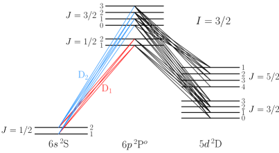
Figure 1: Grotrian diagram for the most general Ba ii model considered in this work, which includes three terms: $6s\,^{2}\mathrm{S}$ (ground term), $5d\,^{2}\mathrm{D}$ (metastable term), and $6p\,^{2}\mathrm{P}^{\mathrm{o}}$ (upper term for the D lines). The latter two consist of two FS levels each. The figure also displays the HFS for the case of the odd isotopes (energies not to scale). The solid lines show the permitted radiative transitions that couple the atomic states of the system. The red and blue lines indicate the transitions pertaining to the D₁ and D₂ lines, respectively.

Except where otherwise noted, we considered the seven stable isotopes of barium throughout this work. Of these, only the two odd isotopes (¹³⁵Ba and ¹³⁷Ba) have a nonzero nuclear spin with $I=3/2$ and thus HFS. Relevant atomic quantities, including the isotopic abundances and shifts and the HFS coefficients can be found in Appendix A. Outside sunspots, Ba i is a minority species and we thus consider all barium atoms to be in the Ba ii and Ba iii stages. In the most general case, we consider five FS levels of Ba ii, namely $6s\,^{2}\mathrm{S}_{1/2}$ (the ground level), $5d\,^{2}\mathrm{D}_{3/2}$ and $5d\,^{2}\mathrm{D}_{5/2}$ (the metastable levels), and $6p\,^{2}\mathrm{P}^{\mathrm{o}}_{1/2}$ and $6p\,^{2}\mathrm{P}^{\mathrm{o}}_{3/2}$ (the upper levels of D₁ and D₂, respectively). The other levels in this ionization stage, which have at least twice the energy of the $6p$ term, are not considered in this work. The Grotrian diagram for this atomic model, including the HFS, can be found in Figure 1. Each HFS level is indicated by its corresponding quantum number $F$. We observe that the energies of the HFS levels of the $5d\,^{2}\mathrm{D}_{5/2}$ metastable level decrease with $F$, as a consequence of its negative magnetic dipole HFS coefficient $\mathcal{A}$ (see Appendix A). The solid lines connecting the various $F$ levels indicate the permitted radiative transitions between them, with red and blue lines pertaining to the D₁ and D₂ lines, respectively. We only account for the ground level of Ba iii, which we consider suitable for determining the ionization balance.

The results of the RT calculations and the corresponding analysis are presented in the following two sections. In Section 3, we study the impact of the metastable levels on the D₁ linear polarization in the absence of magnetic fields, using the HanleRT (del Pino Alemán et al., 2016, 2020) synthesis code. After establishing that the metastable levels modify the amplitude but not the shape of the D₁ scattering polarization, in Section 4 we study the impact of the HFS, the atmospheric model, and the magnetic fields on the polarization patterns of the D₁ line, neglecting the metastable levels. Such numerical investigations were carried out using the RT code for a two-term model introduced in Alsina Ballester et al. (2022).

3 The impact of the 5$d$ metastable levels in the zero-field case

At present, no RT code exists that can simultaneously account for PRD effects, the five above-mentioned atomic levels of Ba ii, the quantum interference between levels belonging to the same term, the HFS, and magnetic fields in the incomplete Paschen-Back (IPB) effect regime. However, we can still gain valuable insights into the physics that shape the intensity and polarization patterns of the Ba ii D lines by employing different numerical approaches that can each account for most of the aforementioned phenomena.

In the present subsection, we made use of the HanleRT numerical code for the synthesis of the intensity and polarization of the D lines. The HanleRT code accounts for scattering processes with PRD effects following the formalism introduced by Casini et al. (2014, 2017a, 2017b) and, in its present version, can consider multi-term atomic systems without HFS. A multi-level modeling that includes the HFS and the quantum interference between the $F$ levels pertaining to a given $J$ level can be achieved with HanleRT by making the formal substitutions $S\rightarrow I$, $J\rightarrow F$, and $L\rightarrow J$, considering the HFS splitting introduced in Appendix A. This treatment neglects quantum interference between FS levels which, as confirmed in 4.2, is a reasonable assumption. This approach is otherwise correct in the absence of magnetic fields. However, in the presence of magnetic fields, the same substitution leads to an incorrect expression of the magnetic Hamiltonian (e.g., Janett et al., 2023). Thus, the calculations with HanleRT presented in this work are restricted to the nonmagnetic case.

For the calculations carried out with HanleRT, we considered only the five most abundant isotopes; we neglected the contribution from the two least abundant stable isotopes because data on the isotopic shifts of their corresponding metastable levels is, as far as we are aware, not presently available. The abundance of the remaining five isotopes was adjusted accordingly. We expect the error incurred to be negligible, because of the low abundance of the omitted isotopes which, moreover, have no nuclear spin.

The population of the ground term, $\mathcal{N}_{\ell}$, was kept fixed during the iterative solution of the non-LTE RT problem, while letting the overall population of the Ba ii levels evolve freely. The reason for this is two-fold. First, the population and ionization balance is calculated considering only the ¹³⁸Ba isotope. This population is then distributed among the isotopes according to their abundances and, for those with HFS, the populations in a given FS level are distributed among the $F$ levels according to their statistical weight. Secondly, the metastable levels are critical for the population balance of the atom. If we were to completely fix the populations, we would be prescribing the populations in the $F$ levels whereas, if we were to leave them completely free (thus ensuring mass conservation), we would not be able to analyze the actual impact on the linear polarization, because the population balance will significantly change the intensity profile. We consider this a reasonable approximation because the population of the lower level is much larger than that of the other levels of the system.

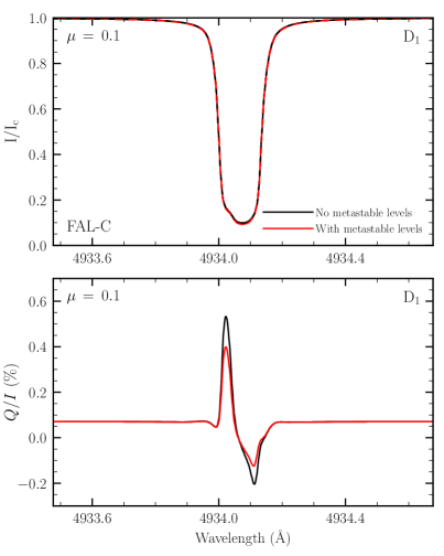
Figure 2: Stokes $I$, normalized to the continuum intensity $I_{\mathrm{c}}$ (upper panel), and fractional linear polarization $Q/I$ profiles (lower panel) of the D₁ line as a function of wavelength. The synthetic profiles are obtained from calculations using the HanleRT code, accounting for partial frequency redistribution (PRD) effects in the angle-averaged (AA) case and accounting for hyperfine structure (HFS) as discussed in the text. The black and red curves correspond to calculations including and neglecting the metastable levels, respectively. For all the figures presented in the main text, the spectral range is $1.2$ Å wide and is centered on the D₁ line. A line of sight (LOS) with $\mu=0.1$ is taken and the reference direction for positive Stokes $Q$ is parallel to the nearest limb.

In Figure 2, we compare the D₁ profiles obtained when including and excluding the $5d\,^{2}\mathrm{D}$ metastable levels in the atomic model. The figure shows the intensity normalized to the continuum intensity at $2$ Å to the red of the line center, $I_{c}$, and the fractional linear polarization pattern $Q/I$. We find an absorption profile in $I/I_{c}$, which is clearly broadened due to the HFS. The inclusion of the metastable levels does not appear to have any impact on the intensity profile (as long as the fixed lower term population is calculated considering the full atomic model); see also Appendix C, where the same behavior is found in the corresponding profile for D₂.

The $Q/I$ pattern presents a positive blue peak and a negative red one, whose amplitudes decrease when accounting for the metastable levels. This may be attributed to the transfer of population imbalances and quantum interference between magnetic sublevels (i.e., atomic polarization) from the $6p\,{}^{2}\mathrm{P}^{\mathrm{o}}_{1/2}$ upper level to the $5d\,^{2}\mathrm{D}_{3/2}$ metastable level. Indeed, we note that the $6p\,{}^{2}\mathrm{P}^{\mathrm{o}}_{1/2}$ level only presents atomic polarization due to the spectral structure of the incident radiation field. The overall shape of the profile obtained when including or neglecting the metastable levels is very similar, with the blue (red) peak remaining positive (negative). This similarity suggests that, if the aim is to qualitatively study the sensitivity of these profiles to specific physical mechanisms such as those driven by the magnetic field, one can reasonably model the Stokes profiles of the D₁ line with a two-term atomic model that neglects the metastable levels (but accounts for the atomic HFS). Indeed, this is the atomic model that is considered in the following sections of this work. Regardless, one must be aware that suitably reproducing spectropolarimetric observations of the Ba ii lines will require the inclusion of such metastable levels. We note that the shape of the D₂ scattering polarization profile is modified by the metastable levels to a far greater degree than that of D₁. The discussion of the D₂ line can be found in Appendix C.

HanleRT can also solve the non-LTE RT problem for polarized radiation accounting for PRD effects while relaxing the AA approximation (i.e., fully accounting for the frequency-angular coupling due to the Doppler effect). Figure 3 shows the comparison between the fractional linear polarization $Q/I$ profiles resulting from calculations with and without the AA approximation. For such calculations, we considered a three-level atomic system (i.e., without the metastable levels) with HFS. We find a good agreement between the two calculations, which highlights the suitability of the AA approximation for modeling the linear polarization pattern of the Ba ii D₁ line, at least in the absence of magnetic fields. This contrasts with the results of the analogous investigation for the Na i D₁ line reported in Janett et al. (2023), in which such approximation was found to have a clear impact on the shape of the $Q/I$ profile. Although it is not shown here, were able to reproduce such findings in the nonmagnetic case using HanleRT. Such differences may be attributed to the fact that the HFS splittings of the upper and lower levels of the Ba ii D₁ line (for the isotopes with nonzero nuclear spin) are more than one order of magnitude larger than those of the corresponding levels of Na i. The separation between the HFS components of the Ba ii D₁ line is proportionally larger, reducing potential spectral overlaps between them due to the Doppler effect. Making the full angle-dependent treatment of scattering processes likewise has no impact on the intensity profile of the Ba ii D₁ line. The synthetic profiles presented in the rest of this work were obtained under the AA approximation.

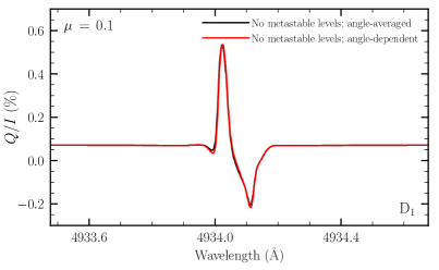
Figure 3: Fractional linear polarization $Q/I$ profiles for the Ba ii line as a function of wavelength. The synthetic profiles were computed using HanleRT, accounting for PRD effects both under the AA approximation (black curve) and considering the fully angle-dependent case (red curve). In the atomic model, the metastable levels were neglected but the HFS was taken into account.

4 The impact of the HFS, atmospheric model, and magnetic fields

In this section we continue investigating the formation of the intensity and polarization profiles of the Ba ii D₁ line in optically thick atmospheres. The numerical approach considered here assumes a two-term atomic model and does not allow for the inclusion of the metastable levels, whose impact on the amplitude of the D₁ scattering polarization is not negligible. On the other hand, it does allow for investigations accounting for the quantum interference between states within the same FS and/or HFS levels while in the presence of magnetic fields of arbitrary strength and orientation.

4.1 Numerical approach

The synthetic Stokes profiles presented in this section were obtained through the following two-step approach.

Step 1: Compute a number of quantities to be used as input for the second step, including the collisional rates, continuum quantities, and the population of the ground term $\mathcal{N}_{\ell}$. Such calculations are carried out by solving the non-LTE problem without polarization using the RH code of Uitenbroek (2001). The considered atomic system includes the ground level of Ba iii and the five levels of Ba ii discussed in Section 2, but not the HFS. Because the metastable levels are included in the calculations in this step, they yield a more accurate value for $\mathcal{N}_{\ell}$ than when considering a two-term atomic system. More details on such calculations can be found in Appendix A.

Step 2: Obtain the synthetic Stokes profiles for the D lines by solving the non-LTE RT problem in the polarized case via the numerical code described in Alsina Ballester et al. (2022). It is suitable for a two-term atomic system and thus does not account for the metastable levels of Ba ii, but it can include the HFS of the odd isotopes. Unless otherwise noted, all seven stable isotopes are considered. The code can account for scattering polarization with both PRD effects under the AA approximation and magnetic fields in the incomplete Paschen-Back effect regime. The ground term is assumed not to have atomic polarization, because elastic collisions with neutral hydrogen are expected to suppress the ground level atomic polarization, as they do for the metastable levels (see Derouich, 2008). Thus, each of the HFS levels of the ground term is populated according to the total $\mathcal{N}_{\ell}$ and its corresponding statistical weight. $\mathcal{N}_{\ell}$ is kept fixed throughout the iterative RT calculation for this step and, because all the RT coefficients are proportional to this value, the problem is linear. The thermal line emissivity is computed as explained in Alsina Ballester et al. (2022). The potential impact of the collisional transfer of atomic polarization between different FS or HFS levels is beyond the scope of this work, and was not taken into account in the calculations for the profiles presented below.

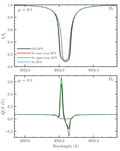
Figure 4: Stokes $I$, normalized to the continuum intensity $I_{\mathrm{c}}$ (upper panel), and $Q/I$ (lower panel) profiles of the D₁ line as a function of wavelength. In all the figures presented in this section, the profiles were calculated following the approach described at the beginning of this section. The colored curves indicate the results of calculations with different treatments of the hyperfine structure (HFS): fully accounting for it (black), accounting only for that of the upper (red) or lower (green) term, or neglecting it entirely (blue). Overlapping curves are dashed for the sake of visibility.

Because we are considering 1D atmospheric models without bulk velocities, the problem is axially symmetric along the local vertical (except in the presence of inclined magnetic fields; see Section 4.4.2). Under such symmetry conditions, and taking the reference direction for positive Stokes $Q$ parallel to the nearest limb, no Stokes $U$ or $V$ are produced and thus the corresponding figures are not shown.

4.2 The impact of HFS

The black curves in Figure 4 represent the D₁ intensity profile normalized to $I_{c}$ (top panel) and the $Q/I$ profile (bottom panel), obtained as described above. Such calculations were carried out in the absence of magnetic fields, considering the FAL-C model and accounting for the HFS of the odd isotopes, as well as for the quantum interference between all states of the upper term. Like in the case of the $Q/I$ profile obtained with HanleRT when neglecting the metastable levels (see Section 3), we find a positive $Q/I$ blue peak and a negative red one. The amplitude of the blue peak is roughly $0.6\%$ (slightly larger than that found with HanleRT) and the amplitude of the red one is just above $0.15\%$ (slightly smaller).

Figure 4 also highlights the impact of the HFS of barium on the intensity and scattering polarization patterns of the D₁ line, by presenting a comparison between the profiles discussed in the previous paragraph, in which the HFS splitting was fully taken into account, and the profiles obtained by neglecting it in the $6s\,^{2}\mathrm{S}$ ground term (red curve), the $6p\,^{2}\mathrm{P}^{\mathrm{o}}$ upper term (blue curve), or both (green curve). Such splittings were neglected by setting to zero the corresponding $\mathcal{A}$ and $\mathcal{B}$ HFS coefficients (see Appendix A).

Only $18\%$ of barium atoms have HFS, but this already leads to a substantial broadening of the D₁ intensity profile (in agreement with Belluzzi & Trujillo Bueno, 2013). This broadening is mostly due to the HFS splitting of the ground term, which is more than one order of magnitude larger than that for the upper level of D₁. The two-peak scattering polarization pattern can only be reproduced by accounting for the HFS and, specifically, that of the ground term. If the latter splitting is neglected, the spectral window spanned by the various HFS components of the D₁ line is very small and the radiation field is effectively flat within this range. As a result, the key mechanism pointed out by Belluzzi & Trujillo Bueno (2013), through which scattering polarization is produced in this intrinsically unpolarizable line, is inhibited. On the other hand, accounting for the HFS of the ground term but neglecting that of the upper level of D₁ leads to an enhancement of the amplitude of the polarization peaks. This enhancement occurs because the quantum interference between the various $F$ levels is maximum if there is no energy separation between them.

We also carried out calculations in which we fully accounted for the HFS but neglected the quantum interference between states pertaining to different $J$ levels of the upper term (i.e., $J$-state interference) and to different $F$ levels of the same $J$ level of the upper term (i.e., $F$-state interference), following Appendix C.7 of Alsina Ballester et al. (2022). Neither $J$- nor $F$-state interference have an appreciable impact on the scattering polarization of the D₁ line and the corresponding profiles are thus not shown. Such results were expected, because the separation between the upper FS levels of the D₁ and D₂ lines is extremely large and even the HFS splitting in the upper level of D₁ is considerably more than one order of magnitude larger than the natural width of the line.

4.3 The sensitivity to the atmospheric model

The semiempirical 1D atmospheric models considered in this work are representative of spatial averages of specific regions of the solar atmosphere and thus cannot account for the full three-dimensional (3D) complexity of the real solar atmosphere. Moreover, bulk velocities are not taken into account in this work, despite the dynamic nature of the Sun. Nevertheless, our modeling can provide valuable insights into the physics that shape the intensity and polarization patterns of non-LTE lines (see, e.g., Faurobert et al., 2009; Smitha et al., 2013, in which the Stokes profiles of the Ba ii D₂ line were synthesized considering various semiempirical models and compared them with observations). Here, we present the synthetic intensity and $Q/I$ profiles of the Ba ii D₁ line obtained with several FAL models other than FAL-C, which was used in the calculations presented above and is representative of an average region of the quiet solar atmosphere. The other considered semiempirical models are FAL-A, which represents relatively faint internetwork regions of the quiet Sun; FAL-F, representative of particularly bright network regions of the quiet Sun; and FAL-P, which corresponds to a typical plage region. We also considered FAL-X, which is representative of an average region of the quiet solar atmosphere, but with considerably lower temperatures than FAL-C in the photosphere and up to the middle chromosphere. Throughout the entire wavelength range taken for the problem (which includes the D₁ and D₂ lines and their nearby continuum), the intensity is highest for model P, then F, then C and X (having very similar values for both models), and is lowest for model A. However, the D₁ intensity profiles, when normalized to $I_{c}$, present a remarkably similar shape for all considered models. The most appreciable differences concern the width of the wings, but even these are minor and are thus not shown here.

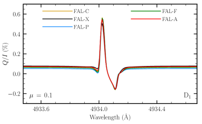
Figure 5: Synthetic $Q/I$ profiles of the D₁ line as a function of wavelength, obtained considering different 1D emiempirical atmospheric models. The colored curves correspond to calculations considering the atmospheric models indicated in the legend.

The differences between the D₁ fractional scattering polarization profiles for the various considered models are also quite modest, as can be seen in Figure 5. Indeed, the largest differences are found between the $Q/I$ profile obtained considering the FAL-X model (with a maximum amplitude of $\sim\!0.50\%$ in the blue peak) and the other models (whose blue peaks reach amplitudes between $\sim\!0.54$ and $0.56\%$).

In order to replicate the spectral smearing due to large-scale velocities typical of the lower chromosphere and the finite resolution of a typical instrument, we convolved the synthetic profiles with a Gaussian function with a FWHM of $70$ mÅ. After such smearing, the $Q/I$ profiles for the various models are indistinguishable at the plot level (figure not shown), and differences are only appreciable in the continuum polarization. We emphasize that even the smeared D₁ profiles still present a positive blue peak and a negative red one, in contrast to the observations reported in Figure 3 of Stenflo et al. (2000). None of the physical ingredients considered in this paper (including metastable levels, angle-dependent PRD, and the magnetic fields, discussed below) can produce a positive red $Q/I$ peak in the D₁ line. For further progress in this respect, we need high-precision spectropolarimetric observations of this line and to include in our theoretical modeling the non-coherent continuum scattering investigated by del Pino Alemán et al. (2014a, b).

Our results indicate that the D₁ line is largely insensitive to the thermodynamical structure of the solar atmosphere and, thus, observable variations in its scattering polarization should be attributed to other factors, such as the presence of a magnetic field. In the future, it will be of interest to investigate the possible sensitivity of the D₁ intensity and polarization signals to changes in atmospheric models that are 3D rather than 1D and dynamic rather than static.

4.4 Magnetic fields

The presence of a magnetic field modifies the energy of the magnetic states $f$ of the Ba ii atom (as illustrated in Figure 2 of Belluzzi et al. 2007b for the ¹³⁷Ba isotope; see also Figure 2 of Belluzzi et al. 2007a). This impacts the polarization of the spectral lines by producing a shift in the $\pi$ and $\sigma$ components of the line and by modifying the quantum interference between $f$ states. A main point of interest in this work is to evaluate the magnetic sensitivity of the polarization patterns of the Ba ii D₁ line, thus providing valuable insights into the potential of this spectral line for diagnostics of chromospheric magnetic fields. Here we present a series of numerical experiments, considering magnetic fields of increasing strength that are either isotropically distributed (see Sect. 4.4.1) or deterministic (see Sect. 4.4.2).

4.4.1 Tangled magnetic fields

We analyze the sensitivity of the D₁ scattering polarization to magnetic fields whose orientation changes at scales smaller than the mean free path of the photons of the line (following Appendix C.6 of Alsina Ballester et al., 2022, where such fields are called micro-structured), with no preferred direction. In particular, we consider such fields with an isotropic distribution of orientations and a fixed strength, which we hereafter refer to as tangled magnetic fields. Such fields do not break the axial symmetry of the problem, and thus they do not give rise to any Stokes $U$ or $V$ signal.

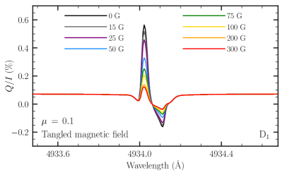
Figure 6: Synthetic $Q/I$ profiles of the D₁ line as a function of wavelength obtained in the presence of tangled magnetic fields. The various colored curves represent the calculations carried out considering the field strengths indicated in the legend.

We carried out calculations for tangled magnetic fields up to $500$ G, although in Figure 6 we only show the $Q/I$ profiles obtained for field strengths up to $300$ G. The intensity profile does not change appreciably within the considered range of field strengths, for which the magnetic splitting is much smaller than the Doppler width, and thus the corresponding figure is not shown. The amplitude of the D₁ scattering polarization begins to decrease appreciably in the presence of fields with strengths of about $15$ G. As the field strength increases further, the polarization amplitude decreases monotonically, but this trend begins to halt at about $200$ G. Although it is not shown in the figure, we also verified that further increases in the field strength beyond $300$ G barely modify the linear polarization amplitude (i.e., saturation is reached). At saturation, the $Q/I$ amplitude of the red peak is $\sim\!0.12\%$, which is approximately $1/5$ of the one obtained in the absence of magnetic fields (roughly $0.60\%$), as expected for the saturation value for isotropic micro-structured fields in a two-level atom (e.g., Trujillo Bueno & Manso Sainz, 1999). Recalling that the D₁ scattering polarization pattern is produced only by the $\sim\!18\%$ of barium isotopes that have nonzero nuclear spin (¹³⁵Ba and ¹³⁷Ba), we focus the discussion on such isotopes and their HFS. We verified numerically that neglecting the magnetic splitting of the ground level does not change the D₁ scattering polarization; its magnetic sensitivity can be mainly attributed to the splitting of the upper level. Indeed, the Larmor frequency at $15$ G is close to $1/5$ of the natural width of the line’s upper level; at that point the splitting between the magnetic states $f$ of any given HFS level of $6p\,^{2}\mathrm{P}^{\mathrm{o}}_{1/2}$ becomes large enough that their interference appreciably decreases, reducing their scattering polarization (the Hanle effect). As the magnetic field increases, so does the splitting between the $f$ states and thus the interference between them becomes weaker. At saturation field strengths, the separation between $f$ states of the same HFSlevel is large enough that the interference between them is negligible.

4.4.2 Deterministic magnetic fields

We also investigate the case of deterministic magnetic fields (i.e., those with a fixed direction rather than an isotropic distribution of orientations), considering first the specific case of horizontal magnetic fields contained in the plane defined by the local vertical and the LOS. For an LOS with $\mu=0.1$, such fields are almost longitudinal. In this case, the problem is no longer axially symmetric and nonzero $U$ and $V$ signals can arise.

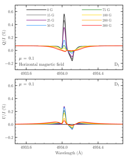
Figure 7: Synthetic $Q/I$ (upper panel) and $U/I$ (lower panel) profiles of the D₁ line as a function of wavelength, obtained in the presence of deterministic horizontal magnetic fields contained within the plane given by the local vertical and the LOS. The various colored curves represent the calculations carried out in the presence of fields with the strengths indicated in the legend.

Figure 7 shows a series of $Q/I$ and $U/I$ profiles obtained in the presence of horizontal magnetic fields with a positive projection onto the LOS and the same strengths considered in Section 4.4.1. Such magnetic fields reduce the amplitude of the $Q/I$ signal to a greater degree than tangled fields of the same strengths. For magnetic fields close to saturation (of $200$ G or stronger), a depolarization pattern is found in $Q/I$. For this geometry, the Hanle effect also gives rise to a $U/I$ signal, whose amplitude increases with magnetic field strength until about $35$ G. For stronger fields, the $U/I$ amplitude instead decreases as the magnetic field reduces the interference between $f$ states.

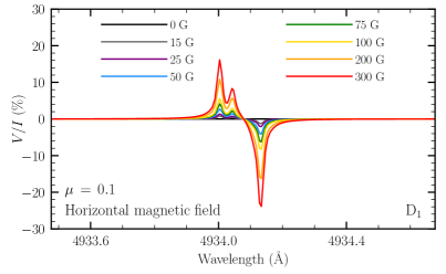
Figure 8: Synthetic $V/I$ profiles of the D₁ line as a function of wavelength, obtained in the presence of the same horizontal magnetic fields considered in the previous figure.

The considered horizontal fields also give rise to a $V/I$ pattern with two positive peaks to the blue of the line center and a negative peak to the red, as illustrated in Figure 8. In the presence of a 15 G magnetic field, the amplitudes of these peaks reach roughly $1\%$ and they increase linearly with field strength within the range considered in this work. This is the behavior typically associated with the Zeeman effect. The double-peak feature found to the blue of the line center is due to the large HFS splitting of the upper and lower levels of the D₁ line. Indeed, we verified that a $V/I$ pattern with a single blue peak is produced instead when the HFS is neglected. This contrasts with the $V/I$ signals found for the K i D₁ line, which arises from a transition between levels with the same $J$ and $F$ quantum numbers, but which could be suitably modeled without accounting for the HFS (see Alsina Ballester, 2022) because its splitting is much smaller than for the analogous levels of Ba ii. We also verified that one cannot suitably apply the magnetograph formula (e.g., Section 9.6 of Landi Degl’Innocenti & Landolfi, 2004) to the Ba ii D₁ line, calculating the Landé factors according to $L$-$S$ coupling (neglecting HFS).

Finally, we evaluated the suitability of the so-called linear Zeeman approximation, that is, neglecting the off-diagonal elements of the magnetic Hamiltonian, which are responsible for the mixing between states with different $J$ or $F$ eigenstates. We verified numerically that, although the mixing between $J$ states can be safely neglected, neglecting the mixing between $F$ states substantially underestimates the amplitude of the circular polarization patterns. The unsuitability of the linear Zeeman approximation had also been reported for spectral lines such as H i Lyman-$\alpha$ (see Alsina Ballester et al., 2019, Appendix A), the Mn i resonance multiplet around $2800$ Å (del Pino Alemán et al., 2022), or the K i D lines (Alsina Ballester, 2022), for which the $J$ or $F$ mixings due to the IPB effect are significant.

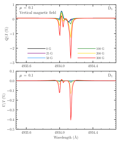
Figure 9: Synthetic $Q/I$ (upper panel) and $U/I$ (lower panel) profiles of the D₁ line as a function of wavelength, obtained in the presence of deterministic vertical magnetic fields. The various colored curves represent the calculations carried in the presence of fields with the strengths as indicated in the legend.

We also considered the case of a vertical deterministic magnetic field, which begins to appreciably impact the linear polarization patterns in the presence of magnetic fields of about $200$ G, as can be seen in Figure 9. Unlike the aforementioned horizontal fields, such vertical fields do not impact the interference between the $f$ states that are degenerate in the nonmagnetic case (the Hanle effect does not operate). Moreover, the energies of the two upper HFS levels of the D₁ line are too far apart for the interference between them to play a meaningful role. Instead, the linear polarization signals can be attributed to the Zeeman effect due to the transverse component of the magnetic field.

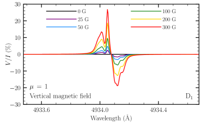
Figure 10: Synthetic $V/I$ profiles of the D₁ line as a function of wavelength, obtained in the presence of the same vertical magnetic fields considered in the previous figure. In order to consider a larger longitudinal component of the magnetic field, for this figure we took an LOS with $\mu=1$.

When considering LOS s close to the disk center, vertical magnetic fields are close to longitudinal and thus give rise to a $V/I$ pattern whose amplitude is proportional to the longitudinal component, as shown in Figure 10. Although the shape of the $V/I$ profile is noticeably different from the one shown in Figure 8 – presenting far wider wing lobes, for instance – there is also a clear double-peak feature due to the HFS. Of course, the magnetograph formula and the linear Zeeman approximation are not suitable for this geometry, either.

5 Conclusions

In this work, we carried out a series of numerical experiments to identify the main physical mechanisms that shape the intensity and polarization patterns of the D₁ line. We obtained the Stokes profiles of these lines through non-LTE RT calculations, considering semiempirical 1D models of the solar atmosphere and atomic models that account for both the D₁ and D₂ lines. Our modeling included both PRD effects and the HFS of the barium isotopes with nuclear spin ($18$ % of the total by abundance). This allowed us to study the scattering polarization arising from the spectral structure of the anisotropic radiation field over the wavelength interval spanned by the various HFS components of D₁. In order to consider relatively large scattering polarization signals, we displayed the resulting Stokes profiles at an LOS with $\mu=0.1$.

Here we evaluated the impact of the metastable levels on the D₁ line in the nonmagnetic case using the HanleRT non-LTE code (del Pino Alemán et al., 2016, 2020). This RT code is designed for a multi-term atomic system without HFS, but through some formal substitutions it can incorporate a multi-level atom with HFS, which neglects the quantum interference between FS levels but is otherwise suitable in the absence of magnetic fields. Although the inclusion of the metastable levels appreciably decreases the amplitude of the $Q/I$ pattern of D₁, they have little impact on its shape. We also verified with HanleRT that the D₁ scattering polarization signal can be suitably modeled making the AA approximation.

For the rest of our investigation, we considered synthetic Stokes profiles calculated using the non-LTE RT code described in Alsina Ballester et al. (2022). Although this code can account for PRD effects only under the AA approximation and cannot account for the metastable levels, it can jointly include the HFS of the odd isotopes of Ba ii and magnetic fields of arbitrary strength and orientation. We find that the very large HFS of the ground term substantially broadens the D₁ intensity profile and is responsible for its two-peak scattering polarization pattern. We also verified that the quantum interference between FS or HFS levels has no significant impact on the linear polarization.

Interestingly, our numerical experiments considering the various FAL semiempirical atmospheric models (which present different stratifications for parameters such as temperature or density) reveal that neither the D₁ continuum-normalized intensity nor the $Q/I$ fractional linear polarization pattern are strongly sensitive to the different models. Thus, most of the variation of its linear polarization can instead be attributed to the magnetic field, enhancing its value for diagnostics of chromospheric magnetic fields. In the future, the variation of the intensity and polarization of the D₁ line should be investigated when considering dynamic models of the solar atmosphere that fully account for its 3D complexity.

In this work we considered tangled and deterministic magnetic fields with strengths of up to $500$ G, although we did not show the Stokes profiles obtained for fields stronger than $300$ G. The considered fields have no appreciable impact on the intensity profile. On the other hand, the linear scattering polarization is clearly sensitive to tangled or horizontal magnetic fields of roughly $15$ G or stronger via the Hanle effect. Tangled magnetic fields of increasing strength progressively depolarize the $Q/I$ signal until reaching saturation at about $300$ G; the $Q/I$ saturation amplitude is approximately $1/5$ of the amplitude in the nonmagnetic case. Deterministic horizontal magnetic fields have a stronger depolarizing effect than tangled fields of the same strength and, at saturation, present an almost completely depolarized signal. In the presence of such fields, the problem is no longer axially symmetric, and thus they give rise to a $U/I$ signal. If the magnetic fields have a substantial longitudinal component, a $V/I$ pattern is produced through the Zeeman effect, with amplitudes that increase linearly with field strength and that reach roughly $1\%$ in the presence of longitudinal fields of $15$ G. Suitably modeling such circular polarization signals requires accounting for the Paschen-Back effect for HFS. The magnetograph formula, assuming $L$-$S$ coupling for the Landé factors, does not yield a reliable estimate of the longitudinal magnetic field from $V/I$. Magnetic fields with transverse components close to $200$ G or larger also produce appreciable linear polarization signals due to the Zeeman effect.

These findings highlight the diagnostic value of spectropolarimetric observations of the Ba ii D₁. However, none of the RT codes currently at our disposal meet all the requirements for a quantitative modeling of the D₁ Stokes profiles. In particular, it is necessary to account for scattering polarization with PRD effects, for the metastable levels and the HFS of the atomic system, for magnetic fields in the IPB effect regime, and for the collisional transfer of population and atomic polarization between all levels of the atomic system. Fortunately, we expect such a code to be developed in the near future. This would also make it possible to model the D₁ together with D₂, whose large scattering polarization is sensitive to considerably weaker magnetic fields, thus offering complementary information about the magnetism in the lower solar chromosphere.

We thank the anonymous reviewer for constructive comments that contributed to improve the manuscript. We gratefully acknowledge the financial support from the European Research Council (ERC) under the European Union’s Horizon 2020 research and innovation program (ERC Advanced grant agreement No. 742265). We also acknowledge support from the Agencia Estatal de Investigación del Ministerio de Ciencia, Innovación y Universidades (MCIU/AEI) under grant “Polarimetric Inference of Magnetic Fields” and the European Regional Development Fund (ERDF) with reference PID2022-136563NB-I00/10.13039/501100011033. T.P.A.’s participation in the publication is part of the Project RYC2021-034006-I, funded by MICIN/AEI/10.13039/501100011033, and the European Union “NextGenerationEU”/RTRP.

Appendix A Atomic quantities

The synthetic Stokes profiles presented in Section 4 were obtained through a two-step calculation in a similar manner as was done in Alsina Ballester et al. (2022). The purpose of the first (or preliminary) step is to provide a set of quantities that are required as input in the second step, in which a two-term atomic model is considered. Such quantities include the rates of elastic and inelastic collisions, continuum quantities (the thermal emissivity, absorption coefficient, and scattering cross-section), and the population of the lower term. They are computed while solving the non-LTE RT problem considering an atomic model with more levels than in the two-term system. For the sake of reducing the computational cost, the problem was solved in the case of unpolarized radiation, using the RH code of Uitenbroek (2001). The considered multilevel atomic system consists of five levels for Ba ii – namely the ground level, the two metastable levels discussed in the main text, and the upper levels of the D₁ and D₂ lines – and of the ground level of Ba iii. It thus includes $5$ continuum transitions and $5$ line transitions. PRD effects are taken into account for the D₁ and D₂ lines but not for the other transitions. We consider this approximation to be suitable for accurately computing the aforementioned quantities. The inelastic collisions (those that induce transitions between different terms) were computed taking into account only the contribution from free electrons, following Seaton (1962). We stored the rate of collisions that couples the upper level of the D₂ line and the ground level, and set it equal to the broadening rate due to inelastic collisions $\Gamma_{I}$, to be used in the second step. Regarding the rate of elastic collisions (those that induce transitions between states that belong to the same term), the quadratic Stark effect contribution from free electrons and singly charged ions was computed following Traving (1960) and the van der Waals contribution from neutral hydrogen and neutral helium was computed according to Unsöld (1955). The resulting broadening rate for the upper level of the D₂ line was stored as the $\Gamma_{E}$ broadening rate, to be used in the second step.

The second step of the calculation yields the synthetic Stokes profiles of the D₁ and D₂ lines shown in Section 4. Such profiles are obtained by solving the non-LTE RT problem in the polarized case using the code described in Alsina Ballester et al. (2022), which considers a two-term system with HFS but cannot account for the metastable levels. The lower term is the $6s\,^{2}\mathrm{S}$ ground term, which has a single FS level whose energy we take to be zero. The upper term $6p\,^{2}\mathrm{P}^{\mathrm{o}}$ consists of two FS levels: the upper level of the D₁ line, with $J=1/2$ and an energy of $20261.561$ cm^-1, and the upper level of the D₂ line, with $J=3/2$ and an energy of $21952.404$ cm^-1. These energies were taken from the NIST database (Kramida et al., 2021). In this framework, all transitions are assumed to have the same line broadening; in addition to the collisional contributions discussed above, this broadening has a radiative contribution $\Gamma_{R}$, which corresponds to the Einstein coefficient for spontaneous emission of the term. Because the D lines share the same lower level, the Einstein coefficient of the two lines are identical if one assumes $L$-$S$ coupling (e.g., Section 7.5 of Landi Degl’Innocenti & Landolfi, 2004). In reality, their experimental values differ substantially (see, e.g., Kramida et al., 2021). We take $\Gamma_{R}=1.03\times 10^{8}$ s^-1, which is the average of the Einstein coefficients for the two lines accounting for the statistical weights of the upper level of each line. In the second step, we take the damping parameter $a$ that enters the RT coefficients to be $a={(\Gamma_{R}+\Gamma_{E}+\Gamma_{I})}/{(4\pi\Delta\nu_{D})}$, where $\Delta\nu_{D}$ is the Doppler width in frequency units.

Table 1: Isotopic abundances and energy shifts

			Isotope shift (cm-1)
	Abundance ($\%$)	$I$	$6p\,^{2}\mathrm{P}^{\mathrm{o}}_{1/2}$	$6p\,^{2}\mathrm{P}^{\mathrm{o}}_{3/2}$
130 Ba	$0.106$	$0$	$1.185\!\times\!10^{-2}$	$1.242\!\times\!10^{-2}$
132 Ba	$0.101$	$0$	$9.303\!\times\!10^{-3}$	$9.837\!\times\!10^{-3}$
134 Ba	$2.417$	$0$	$7.425\!\times\!10^{-3}$	$7.825\!\times\!10^{-3}$
135 Ba	$6.592$	$3/2$	$1.163\!\times\!10^{-2}$	$1.203\!\times\!10^{-2}$
136 Ba	$7.854$	$0$	$5.984\!\times\!10^{-3}$	$6.234\!\times\!10^{-3}$
137 Ba	$11.232$	$3/2$	$9.043\!\times\!10^{-3}$	$9.036\!\times\!10^{-3}$
138 Ba	$71.698$	$0$	$0.000$	$0.000$

The HFS of the atomic system is also included in the second step, in which we account for the seven stable isotopes of barium. Their relative abundance, nuclear spin, and their corresponding isotopic shifts for the upper levels of the D₁ and D₂ lines are displayed in Table 1. The isotopic shifts are given relative to the ¹³⁸Ba. The quantities were taken from Table 1 of Belluzzi et al. (2007b), who themselves took the shifts from Wendt et al. (1984), except for those for the ¹³⁴Ba isotope, which were taken from Wendt et al. (1988).

Table 2: Hyperfine structure coefficients

	135Ba	137Ba
$\mathcal{A}_{6s\,^{2}\mathrm{S}_{1/2}}$ (cm-1)	$1.198\!\times\!10^{-1}$	$1.341\!\times\!10^{-1}$
$\mathcal{A}_{6p\,^{2}\mathrm{P}^{\mathrm{o}}_{1/2}}$ (cm-1)	$2.217\!\times\!10^{-2}$	$2.481\!\times\!10^{-2}$
$\mathcal{A}_{6p\,^{2}\mathrm{P}^{\mathrm{o}}_{3/2}}$ (cm-1)	$3.769\!\times\!10^{-3}$	$4.243\!\times\!10^{-3}$
$\mathcal{B}_{6p\,^{2}\mathrm{P}^{\mathrm{o}}_{3/2}}$ (cm-1)	$1.968\!\times\!10^{-3}$	$3.085\!\times\!10^{-3}$
$\mathcal{A}_{5d\,^{2}\mathrm{D}_{3/2}}$ (cm-1)	$5.567\!\times\!10^{-3}$	$6.329\!\times\!10^{-3}$
$\mathcal{B}_{5d\,^{2}\mathrm{D}_{3/2}}$ (cm-1)	$9.658\!\times\!10^{-4}$	$1.486\!\times\!10^{-3}$
$\mathcal{A}_{5d\,^{2}\mathrm{D}_{5/2}}$ (cm-1)	$-3.581\!\times\!10^{-4}$	$-4.012\!\times\!10^{-4}$
$\mathcal{B}_{5d\,^{2}\mathrm{D}_{5/2}}$ (cm-1)	$1.291\!\times\!10^{-3}$	$1.986\!\times\!10^{-3}$

For the isotopes with nonzero nuclear spin, the energies of the various atomic states depend on the $J$, $F$ and $I$ quantum numbers through the magnetic dipole ($\mathcal{A}$) and electric quadrupole ($\mathcal{B}$) HFS coefficients that enter the Hamiltonian for HFS. The nonzero values of such coefficients are displayed in the four first rows of Table 2, again taken from Table 1 of Belluzzi et al. (2007b), who themselves took the $\mathcal{A}$ coefficients for the ground level from Becker et al. (1981) and the other $\mathcal{A}$ and $\mathcal{B}$ coefficients from Villemoes et al. (1993). The only nonzero $\mathcal{B}$ coefficients correspond to the upper level of the D₂ line. Such coefficients were defined according to the American convention (the expressions of the elements of the HFS Hamiltonian for such convention can be found, for instance, in Appendix B of Alsina Ballester et al., 2022).

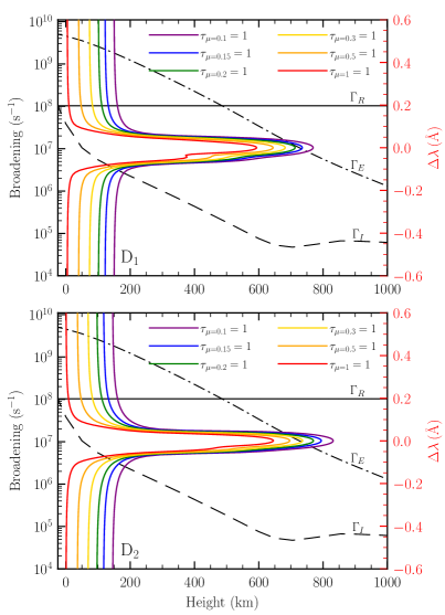
Figure 11: Height at which the optical depth is unity in the FAL-C semiempirical atmospheric model as a function of wavelength, in a $1.2$ Å spectral range centered on the D₁ (upper panel) and D₂ (bottom panel) lines, for the LOS s indicated by the colored curves (see the legend). The black curves represent the broadening due to radiative processes $\Gamma_{R}$ (solid curves), inelastic collisions $\Gamma_{I}$ (dashed curves), and elastic collisions $\Gamma_{E}$ (dashed-dotted curves), as a function of atmospheric height.

The profiles presented in Section 3 were carried out using the HanleRT code, and accounted for the metastable levels $5d\,^{2}\mathrm{D}_{3/2}$ and $5d\,^{2}\mathrm{D}_{5/2}$. Their HFS coefficients, taken from Silverans et al. (1986), are shown in the four bottom rows of Table 2. The isotopic shifts for the five most abundant isotopes, which were the ones considered in such same calculations, were obtained from Villemoes et al. (1993).

Appendix B Formation Height

Figure 11 shows the height in the FAL-C model at which the optical depth $\tau_{\nu}$ is equal to unity. It is shown in two $1.2$ Å-wide spectral ranges, centered on the D₁ (discussed in the main text) and the D₂ lines (discussed in Appendix C). This height is a proxy for the formation height of the line and it is shown for several LOS s. In a 1D atmospheric model, the optical depth is given by $\mathrm{d}\tau_{\nu}=-\eta_{I}\,\mathrm{d}z/\!\mu$, where $z$ is the atmospheric height. $\eta_{I}$ is the absorption coefficient, which was computed following Alsina Ballester et al. (2022), taking $\mathcal{N}_{\ell}$ as obtained in step $1$ of the approach described in Section 4.1. We note that the line core of the D₁ forms above the temperature minumum; the heights at which $\tau=1$ at line center are just below $600$ km in the FAL-C model for an LOS with $\mu=1$ and above $750$ km for $\mu=0.1$. The D₂ forms at slightly higher regions; the height at which its optical depth is equal to unity in the FAL-C model is above $600$ km for $\mu=1$ and above $800$ km for $\mu=0.1$. The $\Gamma_{R}$, $\Gamma_{E}$, and $\Gamma_{I}$ broadenings, shown in both panels as a function of height for reference, were obtained as explained in Appendix A.

Appendix C Analysis of the D₂ Stokes profiles

In the main text, we discussed how various features of the atomic system and properties of the solar atmosphere impact the intensity and linear polarization pattern of the Ba ii D₁ line, illustrated by the synthetic profiles displayed in Sections 3 and 4. The profiles presented therein were calculated considering atomic models that considered not only the D₁ line transitions at $4934$ Å, but also the D₂ line transitions at $4554$ Å. In this appendix, we show the synthetic profiles in the spectral range around the D₂ line instead of D₁. Many such profiles were obtained through the same calculations that yielded the profiles shown in the main text. The FAL-C atmospheric model was considered for all such calculation. Except where otherwise noted, the profiles are shown for an LOS with $\mu=0.1$, taking the reference direction for positive Stokes $Q$ parallel to the nearest limb.

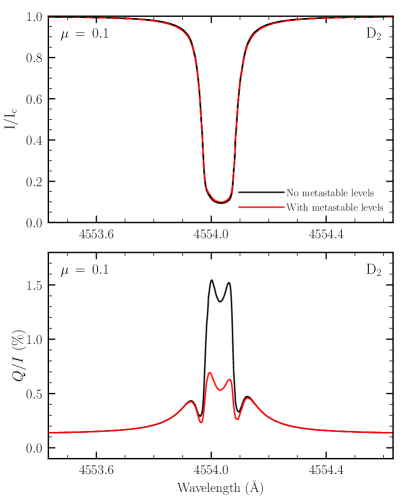
Figure 12: Stokes $I$ (upper panel), normalized to the continuum intensity $I_{\mathrm{c}}$, and $Q/I$ profiles (lower panel) of the D₂ line as a function of wavelength (i.e., in a $1.2$ Å-wide range centered on the D₂ line). The synthetic profiles are obtained from calculations using the HanleRT code, accounting for PRD effects and taking a line of sight (LOS) with $\mu=0.1$. The black curves correspond to the calculations considering a five-level atomic model, including the levels belonging to the $6s\,^{2}\mathrm{S}$ ground term, the $6p\,{}^{2}\mathrm{P}$ term that contains the upper levels of the D lines, and the $5d\,^{2}\mathrm{D}$ metastable term. The red curves correspond to the calculations in which the metastable term is neglected, for which a three-level atomic model is thus considered. In both cases, the HFS of the atomic system is taken into account. The population of the ground level, $\mathcal{N}_{\ell}$, is kept fixed during the iterative calculation.

The D₂ Stokes profiles show in Figure 12 were obtained simultaneously with those presented in Figure 2. Thus, the figure shows the profiles obtained with HanleRT using the atomic models discussed in Section 3, taking into account the HFS of the odd isotopes for all considered levels, both accounting for the metastable levels and neglecting them. Although the $5d\,^{2}\mathrm{D}$ levels do not substantially change the D₂ intensity profile, they have a crucial impact on its linear polarization, decreasing its line-core amplitude by roughly $60\%$. The depolarization due to the metastable levels is far greater than the one reported for the D₁ line, and also leads to a far more apparent change in the shape of its $Q/I$ pattern. For this reason, we deem the calculations presented in Section 4, for which the metastable levels were not included, to be less reliable for the D₂ line than for D₁. Despite this, they may still provide some insights into the sensitivity of this line to the HFS or to the magnetic field. We also verified that the dips found in the line center of the $Q/I$ profile are a consequence of making the AA approximation, implying that a strictly correct modeling of the D₂ line should be carried out through a fully angle-dependent calculation, in contrast to the case of the D₁ line.

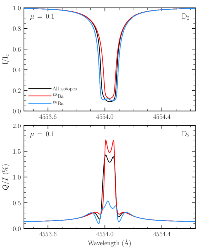
Figure 13: Stokes $I$ (upper panel), normalized to $I_{\mathrm{c}}$, and $Q/I$ profiles (lower panel) of the D₂ line as a function of wavelength. The profiles calculated considering different isotopes of barium are shown with different colored curves. The black curve corresponds to the case in which all seven stable isotopes are considered with their corresponding abundances, whereas the red and blue curves correspond to the cases in which only the ¹³⁸Ba and only the ¹³⁷Ba isotopes were considered, respectively.

In the rest of this appendix, we present profiles using the numerical code discussed in Alsina Ballester et al. (2022), most of them being analogous to those presented in Section 4 for the D₁ line. First, we study the impact of the HFS of the odd isotopes but, unlike in Section 4.2, we do not compare the intensity and linear polarization profiles obtained by accounting for the HFS splitting of different FS levels and neglecting it. Instead, as shown in Figure 13, we compare the profiles obtained considering all seven stable isotopes with their corresponding abundances (see Appendix A), considering only the ¹³⁷Ba isotope, which has nuclear spin $I=3/2$ and HFS, and only ¹³⁸Ba, for which $I=0$ and thus has no HFS. The inclusion of isotopes with HFS leads to a broadening of the absorption profile in intensity, much like what was reported in the D₁ line. A comparison between the linear polarization profiles obtained considering isotopes with $I=0$ and $3/2$ reveals that the very large HFS of barium depolarizes its line-core $Q/I$ by almost a factor $4$. This is consistent with the theoretical depolarization when the quantum interference between different $F$-levels of the upper term is negligible (e.g., Section 10.22 of Landi Degl’Innocenti & Landolfi, 2004). The full scattering polarization amplitude is thus mainly produced by the even isotopes (which have no HFS). This clearly contrasts with the linear polarization pattern of the D₁ line, which is a consequence of the wavelength separation between the HFS components of the odd isotopes.

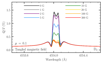
Figure 14: Synthetic $Q/I$ profiles of the D₂ line as a function of wavelength, obtained in the presence of tangled magnetic fields of the various strengths indicated in the legend.

In this Appendix, we also show the D₂ profiles obtained in the presence of both tangled and deterministic magnetic fields, as in Section 4.4, but considering different field strengths in the range between $0$ and $300$ G. The intensity profiles are not appreciably affected by fields of such strengths and thus they are not shown here. The sensitivity of the D₂ linear polarization to tangled magnetic fields (see Section 4.4.1) is illustrated in Figure 14. Such fields preserve the axial symmetry of the problem and thus no $U/I$ or $V/I$ signal is produced. For this line, a depolarization is clearly appreciable in $Q/I$ for fields as weak as $2$ G – considerably lower than those required to modify the D₁ signal. We note that, in contrast to the D₁ line, most of the contribution to the D₂ scattering polarization comes from the roughly $82\%$ of isotopes without HFS. Neglecting HFS, the magnetic field at which the Zeeman splitting of the upper level of D₂ is equal its the natural width (i.e., the Hanle critical field; see e.g., Stenflo, 1994) is approximately $9$ G. This is fully consistent with the behavior displayed in Figure 14. For magnetic fields stronger than $100$ G, the linear polarization amplitude slightly increases, due to the HFS of the odd isotopes, until reaching saturation (for a further discussion on this enhancement, see Section 10.22 of Landi Degl’Innocenti & Landolfi, 2004).

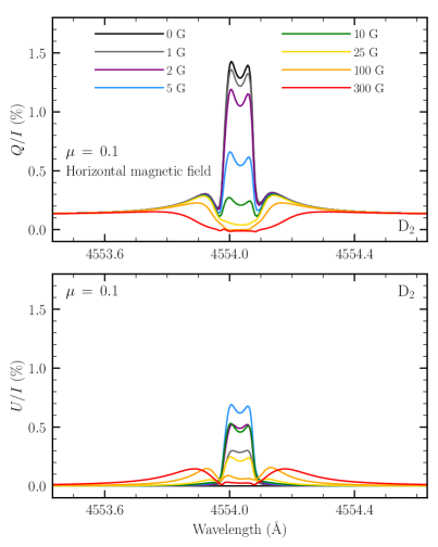
Figure 15: Synthetic $Q/I$ (top panel) and $U/I$ profiles (bottom panel) of the D₂ line as a function of wavelength, obtained in the presence of deterministic horizontal fields contained in the plane defined by the local vertical and the LOS. The various colored curves represent the calculations carried in the presence of magnetic fields of the strengths indicated in the legend.

The synthetic $Q/I$ and $U/I$ profiles of the D₂ line, obtained in the presence of deterministic horizontal magnetic fields, contained in the plane defined by the local vertical and the LOS, are shown in Figure 15. All the considered fields have a positive projection onto the LOS and the various curves indicate the same field strengths as in Figure 14. In the case of horizontal magnetic fields, we observe a stronger depolarization in the line core for a given field strength and a near-zero $Q/I$ value for fields larger than $100$ G, in contrast to the substantial saturation value found for tangled fields. Moreover, horizontal fields induce a rotation of the plane of linear polarization as the quantum interference between nearby $f$-states is modified (i.e., Hanle rotation). A maximum in the $U/I$ amplitude is reached for field strengths close to $5$ G; as the field becomes stronger, the interference between $f$ states becomes smaller and the linear polarization fraction decreases. We see no indication of the loop-like behavior in the polarization diagram (i.e., increases in the $U/I$ amplitude with field strength after having reached a first maximum) that is found in D₂ lines of K i (see Alsina Ballester, 2022) and of Na i (see Section 10.22 of Landi Degl’Innocenti & Landolfi, 2004). We attribute the absence of such loops to the fact that the HFS splitting of the Ba ii isotopes with nuclear spin (required for the loop-like behavior) is large enough that no level crossings are reached until field strengths of roughly $50$ G are considered, at which point the line is almost depolarized.

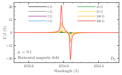
Figure 16: Synthetic $V/I$ profiles as a function of wavelength, in the spectral range centered on D₂, obtained in the presence of the same horizontal fields as in the previous figure.

The considered horizontal fields present a substantial longitudinal component for an LOS with $\mu=0.1$ and, thus, a clear $V/I$ pattern is produced, as shown in Figure 16. The amplitude of the signal increases linearly with the field strength, and reaches roughly $1\%$ for $10$ G fields. Like in the case of the D₁ line, reproducing the shape of the $V/I$ pattern requires accounting for the HFS of the barium atoms. We do not find two distinct blue peaks in the D₂ line, but the HFS splitting does contribute to broadening it appreciably.

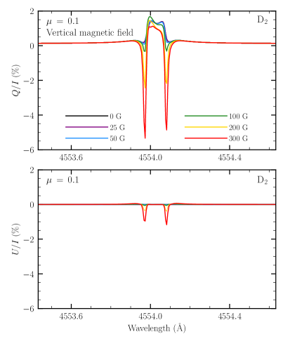
Figure 17: Synthetic $Q/I$ (top panel) and $U/I$ (bottom panel) profiles of the D₂ line as a function of wavelength, in the presence of a vertical magnetic field. The colored curves represent the results of calculations carried in the presence of magnetic fields of the strengths indicated in the legend.

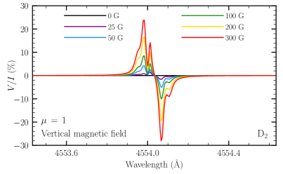
Figure 18: Synthetic $V/I$ profiles as a function of wavelength, in the spectral range centered on D₂, obtained in the presence of a vertical magnetic field, for an LOS with $\mu=1$. The colored curves represent the $V/I$ profiles obtained for the field strengths indicated in the legend.

We also considered the case of a vertical magnetic field, and the resulting linear polarization patterns for an LOS with $\mu=0.1$ are shown in Figure 17. Vertical magnetic fields only modify the quantum interference between states with the same quantum number $f$, and thus its impact on the scattering polarization is much more modest than that of tangled or horizontal magnetic fields. Magnetic fields of about $100$ G or stronger have a large transverse component and introduce a further linear polarization signal due to the Zeeman effect, whose clearest signature in the figure are the negative peaks at either side of the line core, with amplitudes that are noticeably larger than the signals found for the D₁ line for the same geometry and field strengths (see Figure 9). Moreover, vertical magnetic fields also give rise to a circular polarization pattern in the D₂ line due to the Zeeman effect, as is shown in Figure 18. An LOS with $\mu=1$ was selected for this figure in order to consider a completely longitudinal magnetic field. For this geometry, we do find a two-peak structure to the blue of the line center. In contrast to the D₁ $V/I$ profile, the bluemost peak of the D₂ presents a larger amplitude than the one closer to line center. The peak to the red of the line center is much sharper for the D₂ line than for D₁, but it also presents a secondary lobe. We also verified that the amplitude of the D₂ $V/I$ is also substantially underestimated when neglecting the elements of the magnetic Hamiltonian that are off-diagonal in $F$ (making the linear Zeeman approximation, see Section 4.4.2). Likewise, we also find the magnetograph formula to be unsuitable for reproducing the D₂ $V/I$ pattern while considering the $L$-$S$ coupling scheme for the effective Landé factor, although the error incurred is not as large as for the D₁ line.

References

- Alsina Ballester (2022) Alsina Ballester, E. 2022, A&A, 666, A178, doi: 10.1051/0004-6361/202244229
- Alsina Ballester et al. (2019) Alsina Ballester, E., Belluzzi, L., & Trujillo Bueno, J. 2019, ApJ, 880, 85, doi: 10.3847/1538-4357/ab1e41
- Alsina Ballester et al. (2021) —. 2021, Phys. Rev. Lett., 127, 081101, doi: 10.1103/PhysRevLett.127.081101
- Alsina Ballester et al. (2022) —. 2022, A&A, 664, A76, doi: 10.1051/0004-6361/202142934
- Avrett (1995) Avrett, E. H. 1995, in Infrared tools for solar astrophysics: What’s next?, ed. J. R. Kuhn & M. J. Penn, 303–311
- Becker et al. (1981) Becker, W., Blatt, R., & Werth, G. 1981, J. de Phys. Coll., 42, C8
- Belluzzi et al. (2007a) Belluzzi, L., Landi Degl’Innocenti, E., & Trujillo Bueno, J. 2007a, in Astronomical Society of the Pacific Conference Series, Vol. 368, The Physics of Chromospheric Plasmas, ed. P. Heinzel, I. Dorotovič, & R. J. Rutten, 311
- Belluzzi & Trujillo Bueno (2013) Belluzzi, L., & Trujillo Bueno, J. 2013, ApJ, 774, L28, doi: 10.1088/2041-8205/774/2/L28
- Belluzzi et al. (2007b) Belluzzi, L., Trujillo Bueno, J., & Landi Degl’Innocenti, E. 2007b, ApJ, 666, 588, doi: 10.1086/519078
- Casini et al. (2017a) Casini, R., del Pino Alemán, T., & Manso Sainz, R. 2017a, ApJ, 835, 114, doi: 10.3847/1538-4357/835/2/114
- Casini et al. (2017b) —. 2017b, ApJ, 848, 99, doi: 10.3847/1538-4357/aa8a73
- Casini et al. (2014) Casini, R., Landi Degl’Innocenti, M., Manso Sainz, R., Landi Degl’Innocenti, E., & Landolfi, M. 2014, ApJ, 791, 94, doi: 10.1088/0004-637X/791/2/94
- del Pino Alemán et al. (2022) del Pino Alemán, T., Alsina Ballester, E., & Trujillo Bueno, J. 2022, ApJ, 940, 78, doi: 10.3847/1538-4357/ac922c
- del Pino Alemán et al. (2016) del Pino Alemán, T., Casini, R., & Manso Sainz, R. 2016, ApJ, 830, L24, doi: 10.3847/2041-8205/830/2/L24
- del Pino Alemán et al. (2014a) del Pino Alemán, T., Manso Sainz, R., & Trujillo Bueno, J. 2014a, ApJ, 784, 46, doi: 10.1088/0004-637X/784/1/46
- del Pino Alemán et al. (2020) del Pino Alemán, T., Trujillo Bueno, J., Casini, R., & Manso Sainz, R. 2020, ApJ, 891, 91, doi: 10.3847/1538-4357/ab6bc9
- del Pino Alemán et al. (2014b) del Pino Alemán, T., Trujillo Bueno, J., & Uitenbroek, H. 2014b, in Astronomical Society of the Pacific Conference Series, Vol. 489, Solar Polarization 7, ed. K. N. Nagendra, J. O. Stenflo, Z. Q. Qu, & M. Sampoorna, 107
- Derouich (2008) Derouich, M. 2008, A&A, 481, 845, doi: 10.1051/0004-6361:20078888
- Faurobert et al. (2009) Faurobert, M., Derouich, M., Bommier, V., & Arnaud, J. 2009, A&A, 493, 201, doi: 10.1051/0004-6361:200810474
- Fontenla et al. (1993) Fontenla, J. M., Avrett, E. H., & Loeser, R. 1993, ApJ, 406, 319, doi: 10.1086/172443
- Ivanov (1991) Ivanov, V. V. 1991, Analytical Methods of Line Formation Theory: Are they Still Alive? (Dordrecht: Springer Netherlands), 81–104, doi: 10.1007/978-94-011-3554-2_9
- Janett et al. (2023) Janett, G., Alsina Ballester, E., Belluzzi, L., del Pino Alemán, T., & Trujillo Bueno, J. 2023, ApJ (submitted)
- Kramida et al. (2021) Kramida, A., Ralchenko, Y., Reader, J., & NIST ASD Team. 2021, NIST Atomic Spectra Database (version 5.9), Gaithersburg, MD, National Institute of Standards and Technology [Online]. Available: https://physics.nist.gov/asd
- Landi Degl’Innocenti & Landolfi (2004) Landi Degl’Innocenti, E., & Landolfi, M. 2004, Polarization in Spectral Lines, Vol. 307 (Dordrecht: Springer), doi: 10.1007/978-1-4020-2415-3
- López Ariste et al. (2009) López Ariste, A., Asensio Ramos, A., Manso Sainz, R., Derouich, M., & Gelly, B. 2009, A&A, 501, 729, doi: 10.1051/0004-6361/20078154
- Ramelli et al. (2009) Ramelli, R., Bianda, M., Trujillo Bueno, J., Belluzzi, L., & Landi Degl’Innocenti, E. 2009, in Astronomical Society of the Pacific Conference Series, Vol. 405, Solar Polarization 5: In Honor of Jan Stenflo, ed. S. V. Berdyugina, K. N. Nagendra, & R. Ramelli, 41, doi: 10.48550/arXiv.0906.2320
- Rees & Saliba (1982) Rees, D. E., & Saliba, G. J. 1982, A&A, 115, 1
- Seaton (1962) Seaton, M. J. 1962, Proceedings of the Physical Society, 79, 1105, doi: 10.1088/0370-1328/79/6/304
- Silverans et al. (1986) Silverans, R. E., Borghs, G., de Bisschop, P., & van Hove, M. 1986, Phys. Rev. A, 33, 2117, doi: 10.1103/PhysRevA.33.2117
- Smitha et al. (2013) Smitha, H. N., Nagendra, K. N., Sampoorna, M., & Stenflo, J. O. 2013, J. Quant. Spec. Radiat. Transf., 115, 46, doi: 10.1016/j.jqsrt.2012.09.002
- Stenflo (1994) Stenflo, J. 1994, Solar Magnetic Fields: Polarized Radiation Diagnostics, Vol. 189 (Dordrecht: Springer), doi: 10.1007/978-94-015-8246-9
- Stenflo & Keller (1997) Stenflo, J. O., & Keller, C. U. 1997, A&A, 321, 927
- Stenflo et al. (2000) Stenflo, J. O., Keller, C. U., & Gandorfer, A. 2000, A&A, 355, 789
- Traving (1960) Traving, G. 1960, ZAp, 49, 231
- Trujillo Bueno & del Pino Alemán (2022) Trujillo Bueno, J., & del Pino Alemán, T. 2022, ARA&A, 60, 415, doi: 10.1146/annurev-astro-041122-031043
- Trujillo Bueno & Manso Sainz (1999) Trujillo Bueno, J., & Manso Sainz, R. 1999, ApJ, 516, 436, doi: 10.1086/307107
- Trujillo Bueno et al. (2004) Trujillo Bueno, J., Shchukina, N., & Asensio Ramos, A. 2004, Nature, 430, 326, doi: 10.1038/nature02669
- Uitenbroek (2001) Uitenbroek, H. 2001, ApJ, 557, 389, doi: 10.1086/321659
- Unsöld (1955) Unsöld, A. 1955, Physik der Sternatmospharen, mit besonderer Berücksichtigung der Sonne. (Berlin: Springer)
- Villemoes et al. (1993) Villemoes, P., Arnesen, A., Heijkenskjold, F., & Wannstrom, A. 1993, Journal of Physics B Atomic Molecular Physics, 26, 4289, doi: 10.1088/0953-4075/26/22/030
- Wendt et al. (1984) Wendt, K., Ahmad, S. A., Buchinger, F., et al. 1984, ZAp, 318, 125, doi: 10.1007/BF01413460
- Wendt et al. (1988) Wendt, K., Ahmad, S. A., Ekström, C., et al. 1988, Zeitschrift fur Physik A Hadrons and Nuclei, 329, 407, doi: 10.1007/BF01294345