New Physics couplings from angular coefficient functions of
Pietro Colangelo
pietro.colangelo@ba.infn.itIstituto Nazionale di Fisica Nucleare, Sezione di Bari, via Orabona 4, 70126 Bari, Italy
Fulvia De Fazio
fulvia.defazio@ba.infn.itIstituto Nazionale di Fisica Nucleare, Sezione di Bari, via Orabona 4, 70126 Bari, Italy
Francesco Loparco
francesco.loparco1@ba.infn.itIstituto Nazionale di Fisica Nucleare, Sezione di Bari, via Orabona 4, 70126 Bari, Italy
Nicola Losacco
nicola.losacco@ba.infn.itIstituto Nazionale di Fisica Nucleare, Sezione di Bari, via Orabona 4, 70126 Bari, Italy
Dipartimento Interateneo di Fisica ”Michelangelo Merlin”, Università degli Studi di Bari, via Orabona 4, 70126 Bari, Italy
Abstract
The Belle Collaboration has recently measured the complete set of angular coefficient functions for the exclusive decays , with , in four bins of the parameter , with the lepton pair momentum [1].
Under the assumption that physics beyond the Standard Model does not contribute to such modes, the measurements are useful to determine the hadronic form factors describing the matrix elements of the Standard Model weak current, and to improve the determination of .
On the other hand, they can be used to assess the impact of possible new physics contributions. In a bottom-up approach, we extend the Standard Model effective Hamiltonian governing this mode with the inclusion of the full set of Lorentz invariant d=6 operators compatible with the gauge symmetry of the theory. The measured angular coefficient functions can tightly constrain the couplings in the generalized Hamiltonian. We present the first results of this analysis, discussing how improvements can be achieved when more complete data on the angular coefficient functions will be available.
††preprint: BARI-TH/754-24
I Introduction and framework
In the search of signals from physics beyond the Standard Model (SM), a few tensions between SM expectations and measurements have emerged in the flavour sector
[2, 3].
In particular, in addition to processes suppressed at tree-level in SM, which are highly sensitive to virtual contribution of heavy quanta [4], also charged current processes are under scrutiny after the emergence of anomalies in the ratios in BaBar Collaboration [5] and subsequent analyses [6, 2].
The possibility of relating such anomalies to the tensions for the different determinations of makes the investigation of such processes even more intriguing [7].
The angular coefficient functions in the fully differential decay distribution
are suitable observables to look for the effects of new physics (NP) [8, 9, 10, 11, 12].
The Belle Collaboration has recently reported the measurement of the complete set of such functions in four bins of the hadronic recoil parameter , with [1]. Here, we want to consider the role of NP in this process using theoretical expressions that can be applied also to other modes [13, 14].
We make use of the Standard Model Effective Field Theory (SMEFT) as a model-independent framework to analyze NP contributions to beauty hadron decays [15, 16]. If the NP scale is much larger than the electroweak scale, the new massive degrees of freedom can be integrated out providing an effective Hamiltonian in terms of SM fields, invariant under the SM gauge group.
In the extended Hamiltonian new operators not present in the SM appear, suppressed by powers of . At these are dimension-six operators. Among these, those relevant for the present study are four fermion operators.
To describe the modes , with a meson comprising an up-type quark , we consider the generalized effective Hamiltonian
with the Fermi constant and the relevant element of the Cabibbo-Kobayashi-Maskawa (CKM) matrix. Besides the SM term, the low energy Hamiltonian (I) comprises NP operators with complex lepton-flavour dependent coefficients. The scalar operator does not contribute if is a vector meson, as in the present case.
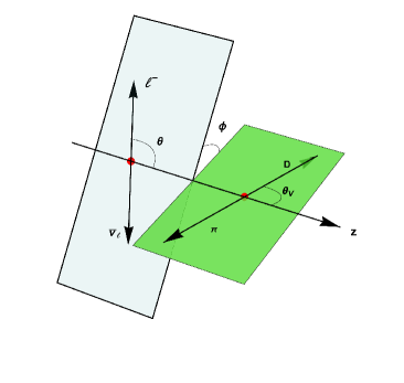
Figure 1: Kinematics of .
Choosing the kinematics indicated in fig. 1, the fully differential decay width reads:
with
and the three-momentum of the meson (here ) in the meson rest-frame.
The angular coefficient functions in (I) depend on the couplings , on (or ) and on the hadronic form factors:
for ,
and for
(5)
In SM such functions are expressed in terms of helicity amplitudes:
(6)
with the form factors defined in the appendix A.
For NP operators the amplitudes are also introduced:
(7)
The form factors are also defined in appendix A. The expressions of all coefficient functions are in the appendix B.
II Constraints on NP couplings from Belle measurement
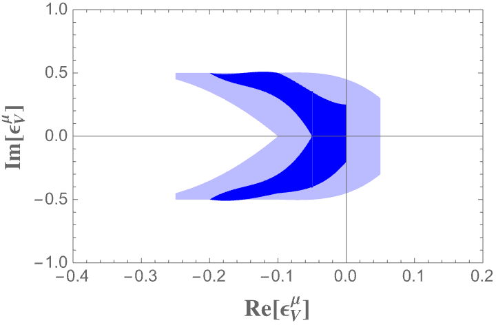
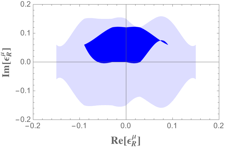
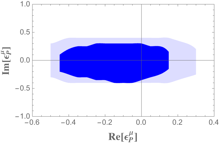
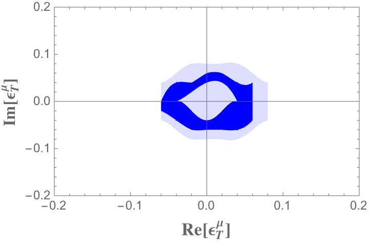
Figure 2: NP couplings obtained from the Belle measurement of the angular coefficient functions of . The light region corresponds to requiring that the theoretical results agree with the experimental data at 2.5 . The dark region corresponds to the values obtained minimizing the reduced .
The comparison of the Belle measurement [1] to the theoretical expressions in the previous section allows us to constrain the couplings in the generalized Hamiltonian (I).
Before presenting the analysis, we point out that
i) the coefficient functions defined in the previous section are related to the coefficient functions in [1], denoted as , through , with ; ii) the angle in [1] corresponds to in our notation, therefore we have for , and for all the other coefficients;
iii) the Belle Collaboration provides the angular coefficient functions in four bins of , defining and , where . The factor corresponds, modulo a constant, to the integrated width.
To get information on the effective couplings we proceed as follows. From fig. 1 of [1] we obtain the values of the coefficients in the four bins , , , (for such an information the Collaboration has not provided in [1] the table of numerical results and the error covariance matrix).
Next, we consider the products .
Using the results in appendix B and fixing the parameter to reproduce the measured branching ratio quoted in [17], we calculate the expressions of the integrals of the coefficient functions in each bin of , . The dependence of the hadronic form factors is needed to perform the integrals: we use the CLN parametrization [18] with the parameters obtained in [19]. The details on the reconstruction of the form factors and on the choice of the parameters can be found in [8].
We require that , with a number of standard deviations to be fixed; is the error of the Belle result for each multiplied by the corresponding bin width. We have a total of 48 constraints, i.e. the integrals over 4 bins for 12 angular coefficients. Since the data refer to the muon channel, we determine the set ) (set 1) that can simultaneously satisfy all constraints, within the inital ranges for . We find that the smallest value of for which all constraints are fulfilled is . Within this set of parameters we select those (set 2) corresponding to the minimum of the function , with and .
The results are in fig. 2: the light region corresponds to the parameters in set 1, while the dark region to the parameters in set 2.
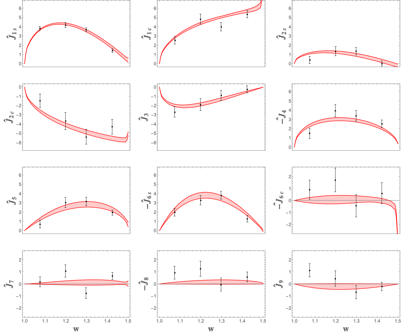
The agreement with data can be appreciated from fig. 3 which includes the Belle points together with the angular coefficient functions obtained using the determined couplings. The remarkable result is that, while the SM point with all new couplings equal to zero is allowed, it does not belong to the region of minimum , and there is the possibility of values different from zero in .
This observation will be strengthened when the table of measurements and the error covariance matrix will be available.
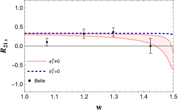
Other observables are sensitive to the effects of the new operators in (I). In particular, an interesting observable is the ratio
(8)
Figure 3: Angular coefficient functions in Eq. (I) for . The shaded regions correspond to the results obtained using the determined couplings, the points are the Belle measurements [1]. Figure 4: Ratio
in Eq. (8)
for (dashed line) and varying in the range displayed in fig. 2 (shaded region).
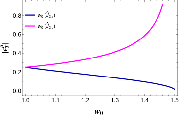
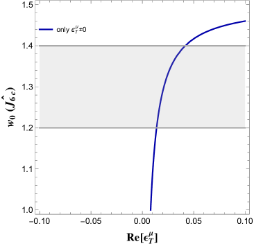
Figure 5: as a function of the position of the zero of the ratio (blue curve) and (magenta curve) for .
Indeed, as obtained using the expressions in appendix B, the angular coefficient functions , hence , do not depend on . For vanishing their ratio would be independent of the form factors and insensitive to . Therefore, the ratio (8) might signal the tensor operator. This is displayed in fig. 4 which shows that for non-vanishing the ratio can have a zero for in the range in the muon channel.
The structure of the angular coefficients provides insights on the possibility that
is the only non vanishing new coupling. In particular, for one finds that both and might have a zero. This is depicted in fig. 5. This figure shows that if should have a zero while should not, and viceversa. They cannot have a zero simultaneously.
Although the Belle data are not precise enough to draw definite conclusions, they seem to exclude the presence of a zero in and are compatible with the presence of a zero of in the last bin of .
Figure 6: as a function of the position of the zero of for , obtained from Eq. (9).
Other angular coefficient functions provide us with further information. If the only non-vanishing NP coupling is , would display a zero at a value given by the relation
(9)
The position of the zero of would fix . This is shown in fig. 6, where the continuous curve corresponds to the relation (9), while the gray band is the range of where the zero of should be found according to the Belle measurement. This corresponds to small values of , consistently with the results for and .
III Conclusions
The measurement of the full set of angular coefficient functions in constrains the set of NP coefficients in the generalized low energy Hamiltonian. In particular, the possibility that some NP coefficients are different from zero emerges as a first evidence on the basis of the information available in [1]. The public table of measurements and the covariance error matrix are eagerly waited, in order to corroborate this preliminary indication.
Acknowledgements.
We thank M. Prim and M. Rotondo for discussions.
This study has been carried out within the INFN project (Iniziativa Specifica) SPIF.
The research has been partly funded by the European Union – Next Generation EU through the research grant number P2022Z4P4B “SOPHYA - Sustainable Optimised PHYsics Algorithms: fundamental physics to build an advanced society” under the program PRIN 2022 PNRR of the Italian Ministero dell’Universitá e Ricerca (MUR).
Appendix A Hadronic matrix elements
The matrix elements are parametrized as:
(A.1)
with the condition
(A.2)
and
(A.3)
Appendix B Angular coefficient functions
Table 1: Angular coefficient functions in the 4d decay distribution for the SM.
Table 2: Angular coefficient functions for : NP term with the R operator, and interference SM-NP with R operator.
Table 3: Angular coefficient functions for : NP term with the P operator, and interference SM-NP with P operator.
0
0
0
0
Table 4: Angular coefficient functions for : NP term with the T operator and interference SM-NP with T operator.
0
0
0
0
Table 5: Angular coefficient functions for : P-R, R-T and P-T interferences.