Theory of momentum-resolved magnon electron energy loss spectra: The case of Yttrium Iron Garnet

Abstract

We explore the inelastic spectra of electrons impinging in a magnetic system. The methodology here presented is intended to highlight the charge-dependent interaction of the electron beam in a STEM-EELS experiment, and the local vector potential generated by the magnetic lattice. This interaction shows an intensity $10^{-2}$ smaller than the purely spin interaction, which is taken to be functionally the same as in the inelastic neutron experiment. On the other hand, it shows a strong scattering vector dependence ($\kappa^{-4}$) and a dependence with the relative orientation between the probe wavevector and the local magnetic moments of the solid. We present YIG as a case study due to its high interest by the community.

Keywords

Spintronics, Magnonics, antiferromagnetic, yttrium iron garnet, YIG

I Introduction

For quite some time, Moore’s Law, especially the concern about its potential end, has driven research into new computing approaches beyond traditional CMOS technology. One approach that has attracted attention is to use the spin degree of freedom to substitute or integrate with the current electronic computation. To this objective, magnonics has been extensively studied, it encompasses the study of fundamental properties of magnons, which are quanta of the dynamic eigen-excitation of magnetically ordered materials in the form of spin-waves Mahmoud2020 ; Barman_2021 .

To systematically investigate the generation, manipulation, and identification of spin-waves, or magnons, there is a requisite focus on improving the methodologies for both exciting and probing these phenomena. Magnons are commonly studied by inelastic neutron scattering (INS) techniques, time-resolved Kerr microscopy Kerr2017 , and Brillouin light scattering (BLS) BLS2015 . While these techniques probe the energy-momentum dispersion of magnons with high energy resolution, their spatial resolution is fundamentally limited to hundreds of nanometres.

Over the past decade, meV-level STEM-EELS has made significant strides, achieving atomic-level contrastHage2019 , detecting spectral signatures of individual impurity atoms Hage2020 , and conducting spatial- and angle-resolved measurements on defects in crystalline materials Hoglund2022-qm .

The method’s potential expansion into studying magnons is anticipated due to the overlapping energy range with vibrational modes in solid-state materials. Despite the weaker interaction of magnetic moments with the electron beam compared to the Coulomb potential, by up to 3 or 4 orders of magnitude, which makes their detection challenging,Loudon2012 ; Rusz2021 recent advancements in hybrid-pixel detectors, leading to a drastic improvement in the dynamic range and low background noise, with signals a mere 10^-7 of the full beam intensity readily detectable PLOTKINSWING2020 , and improved monochromator and spectrometer design, resulting in increased energy resolutions in particular at lower acceleration voltages (4.2meV at 30kV KRIVANEK201960 ), offer enhanced sensitivity and signal detection, making the exploration of magnon excitation feasible in experimental settings.

Theoretical approaches for evaluating the EEL spectra have focused on spin-polarized probes and Low-energy electrons in a surface reflection geometry (REELS), in bulk materials. In our case we will explore the effects of non-spin-polarized beam in the meV-level STEM-EELS apparatus, using YIG as a prototypical material, accounting for the electron’s interaction with the vector potential produced by the magnons in the system.

II Methods

The evaluation of the inelastic scattering of electrons by magnons requires the evaluation of the doubly differential cross-section, which evaluates the relative intensity of scattered particles into a solid angle $d\Omega$, with a wavevector in a small range around $\mathbf{k}_{1}$ given by $d\mathbf{k}_{1}$. Assuming N scatterers in the target, and a monochromatic beam with wavevector $\mathbf{k}_{o}$ in the z-direction with a current density $(J_{0})_{z}$. This relative intensity can be written as,

$$\frac{d^{2}\sigma}{d\Omega d\mathbf{k}_{1}}=\frac{1}{N}\frac{N_{0}V\sum_{n_{0},n_{1}}P_{n_{0}}\mathbf{k}_{1}^{2}|\langle n_{1},\mathbf{k}_{1}\rvert H_{inter}\lvert n_{0},\mathbf{k}_{0}\rangle|^{2}\delta(E_{n_{0}}+E_{0}-E_{n_{1}}-E_{1})}{(2\pi)^{2}\hbar(j_{0})_{z}}$$ (1)

where we are denoting a scattering process where the system undergoes a transition from state $n_{0}$ to $n_{1}$ with energies $E_{0}$ and $E_{1}$, respectively, simultaneously the scattered particle changed its momentum from $k_{0}$ with energy $E_{0}$ to $k_{1}$ with energy $E_{1}$. The interaction between the particle and the material is encapsulated by the interaction Hamiltonian $H_{inter}$, while the current density of the particle beam along the z-direction is denoted by $(j_{0})_{z}$. Here, $P_{n_{0}}$ signifies the probability of the material to be in state $n_{0}$ before any scattering event. While $N$, represents the number of statterers, $N_{0}$ is the number of particles in state $k_{0}$, and $V$ is the volume of the unit cell.

The choice of $H_{inter}$ is the central point of the discussion. In our case, we are interested in the interaction of an electron beam with the magnetic structure of the system. Disregarding the charge, the problem returns to a similar situation as to the INS, the usual interaction is taken in terms of an interaction between the magnetic field generated by the intrinsic magnetic moment of the electrons and the orbital angular momentum. This interaction leads to an exchange-like term and a term involving the sample’s electron motion. In the case of orbital quenched systems only the former terms is taken in account. In our approach, the interaction will be assumed to be given by the vector potential deriving from the magnons in the solid and its effect on the canonical momentum of the passing probe electrons. This interaction is only present in the case of electrons as a probe. We will then focus on the methodological development of this contribution to the total EELS by magnons.

The interaction can be written by ignoring the weaker $\hat{A}^{2}$ terms and assuming orbital quenching, we have Mendis2022 ,

$$H_{inter}=i\left(\frac{\mu_{0}\mu_{B}^{2}}{\pi}\right)\sum_{j}\left[\hat{S}_{j}\times\frac{\mathbf{r}-\mathbf{r}_{j}}{|\mathbf{r}-\mathbf{r}_{j}|^{3}}\right]\cdot\nabla_{r}$$ (2)

where we have the spin operator in site $N$ is given by $\hat{S}_{j}$, $\mu_{B}$ is the Bohr magneton and $\mu_{0}$ is the permeability of free space.

With a semi-classical approach to the spin operators, justified by assuming that $S>>1$, we can note our spins in the laboratory frame as:

$$\mathbf{S}_{i}=S(sin\theta_{i}cos\phi_{i},sin\theta_{i}sin\phi_{i},cos\theta_{i})$$ (3)

with $\displaystyle\theta$ being the polar angle in spherical coordinates and $\displaystyle\phi$ the azimuthal angle. We can perform a transformation to the local reference frame of the spin, given by:

$$\mathcal{R}_{j}^{-1}= \begin{pmatrix}cos\theta_{j}cos\phi_{j}&-sin\phi_{j}&sin\theta_{j}cos\phi_{j}\\ cos\theta_{j}sin\phi_{j}&cos\phi_{j}&sin\theta_{j}sin\phi_{j}\\ -sin\theta_{j}&0&cos\theta_{j}\end{pmatrix}$$ (4)

$$= \begin{pmatrix}A_{11}^{j}&A_{12}^{j}&A_{13}^{j}\\ A_{21}^{j}&A_{22}^{j}&A_{23}^{j}\\ A_{31}^{j}&A_{32}^{j}&A_{33}^{j}\end{pmatrix}$$

Which allows us to write $\overline{\mathbf{S}}_{i}=\mathrm{U}_{i}\cdot\mathbf{S}_{i}$. In this notation, $\overline{\mathbf{S}}_{i}$ refers to the local reference frame and $\mathbf{S}_{i}$ is the laboratory reference frame. Hence we can substitute in our interaction Hamiltonian$\mathbf{S}_{i}=\mathrm{U}_{i}^{-1}\cdot\overline{\mathbf{S}}_{i}$, such that,

$$H_{inter}=i\left(\frac{\mu_{0}\mu_{B}^{2}}{\pi}\right)\sum_{j}\left[\mathcal{R}_{j}^{-1}\cdot\overline{\mathbf{S}}_{j}\times\frac{\mathbf{r}-\mathbf{r}_{j}}{|\mathbf{r}-\mathbf{r}_{j}|^{3}}\right]\cdot\nabla_{r}$$ (5)

Assuming that the scattering particle doesn’t interact with the system before or after the scattering event, i.e., no multiple scattering events, we can write the total wave function as a product between a plane wave and the magnetic states,

$$\lvert\mathbf{k_{i}},n_{i}\rangle\rightarrow\lvert\mathbf{k_{i}}\rangle\lvert n_{i}\rangle$$ (6)

for $i=0,1$. Here we have, $\lvert\mathbf{k_{i}}\rangle=e^{-ik_{i}\cdotp r}$ being the state of the probing beam, while $\lvert n_{i}\rangle$, represents the state of the solid, which for our purposes is only transiting between magnetic states, such that $H_{0}\lvert n_{i}\rangle=E_{i}\lvert n_{i}\rangle$ with $H_{0}$ being the Heisemberg Hamiltonian.

To further our analysis, let’s focus on the interaction term. Substituting (2) in the Fermi’s Golden rule present in (1), while taking (6) into account we have,

$$\langle n_{0},\mathbf{k}_{0}\rvert H_{inter}\lvert n_{1},\mathbf{k}_{1}\rangle= \left(\frac{\mu_{0}\mu_{B}^{2}}{\pi}\right)\langle n_{1}\rvert i\int\sum_{j}e^{-i(\mathbf{k}_{1}-\mathbf{k}_{0})\cdot\mathbf{r}}$$ (7)

$$\left[\left(\mathcal{R}_{j}^{-1}\cdot\overline{\mathbf{S}}_{j}\right)\times\frac{\mathbf{r}-\mathbf{r}_{j}}{|\mathbf{r}-\mathbf{r}_{j}|^{3}}\right] \cdot\mathbf{k}_{0}d\mathbf{r}\lvert n_{0}\rangle$$

taking the integral over $d\mathbf{r}$ which is the same as taking the Fourier transform, where we used the result,

$$FT\left[\frac{\mathbf{r}-\mathbf{r}_{j}}{|\mathbf{r}-\mathbf{r}_{j}|^{3}}\right]=\frac{2i\mathbf{q}}{q^{2}}e^{i\mathbf{q}\cdot\mathbf{r}_{j}}$$ (8)

where we defined $\mathbf{q}=(\mathbf{k}_{1}-\mathbf{k}_{0})$. Then the summation over $j$ results in a discrete Fourier transform of the spin-operators, leading to the result,

$$\langle n_{0},\mathbf{k}_{0}\rvert H_{inter}\lvert n_{1},\mathbf{k}_{1}\rangle= -\left(\frac{\mu_{0}\mu_{B}^{2}\sqrt{N}}{\pi}\right)\langle n_{1}\rvert\sum_{r}e^{-i\mathbf{q}\cdot\mathbf{r}_{r}}$$ (9)

$$\left[\left(\mathcal{R}_{r}^{-1}\cdot\overline{\mathbf{S}}_{q}^{(r)}\right)\times\frac{2\mathbf{q}}{q^{2}}\right] \cdot\mathbf{k}_{0}\lvert n_{0}\rangle$$

where the summation over $r$ labels the sum of magnetic moments in the lattice within the unit cell. Finally, we will use the Holstein-Primakoff transformation in the spin-wave approximation, with $\displaystyle S_{r}$ as the magnitude of the spin angular momentum, given by, in Fourier space,

$$\begin{cases}S_{q}^{x(r)}&=\frac{\sqrt{2S^{(r)}}}{2}\left(a_{q}^{(r)}+a_{q}^{\dagger(r)}\right)\\ S_{q}^{y(r)}&=\frac{\sqrt{2S^{(r)}}}{2i}\left(a_{q}^{(r)}-a_{q}^{\dagger(r)}\right)\\ S_{q}^{z(r)}&=S^{(r)}-a_{q}^{\dagger(r)}a_{q}^{(r)}\end{cases}$$ (10)

Noting that $\displaystyle a_{q}^{\dagger(r)}\lvert n_{0}\rangle=\sqrt{N_{q}+1}\lvert n_{1}\rangle$ while $\displaystyle a_{q}^{(r)}\lvert n_{0}\rangle=0$. In this sense we have two separate contributions to the spectra, one coming from the creation of a magnon and one from the destruction of one, referring to the possibility of Stokes and anti-Stokes scattering, note that with this $S_{q}^{z(r)}$ doesn’t contribute to the inelastic scattering process. Focusing on Stakes scattering only we will only keep the creation operators. Finally, for a general unit cell for both colinear and non-colinear spin-structures, the application of the creation and annihilation operators presume a diagonal Hamiltonian, hence we need to make sure that we have a consistent diagonalisation method for all these cases. To achieve this we will use the method outlined in Thz_Spectroscopy Bearisto doNascimento2023 . In the case of the Heisenberg Hamiltonian in the second quantization under the spin-wave approximation, we can write,

$$H_{2}=v^{\dagger}_{\mathbf{q}}\cdot\textbf{L}\cdot v_{\mathbf{q}}$$ (11)

where we defined:

$$v^{\dagger}=(a^{(1)\dagger}_{\mathbf{q}},...,a^{(M)\dagger}_{\mathbf{q}}|a^{(1)}_{-\mathbf{q}},...,a^{(M)}_{-\mathbf{q}})$$ (12)

We diagonalize $L(q)$ with the unitary transformation $L^{\prime}(q)=UL^{\prime}(q)U^{\dagger}$, where $U^{\dagger}$ is a matrix which columns are the eigenvectors of $L$, this allow us to write:

$$H_{2}=\vec{v}^{\dagger}U^{\dagger}U\textbf{L}U^{\dagger}U\vec{v}=w^{\dagger}L^{\prime}w$$ (13)

having defined $w^{\dagger}=\vec{v}^{\dagger}U^{\dagger}$ given by:

$$w^{\dagger}=(\alpha^{(1)\dagger}_{\mathbf{q}},...,\alpha^{(M)\dagger}_{\mathbf{q}}|\alpha^{(1)}_{-\mathbf{q}},...,\alpha^{(M)}_{-\mathbf{q}})$$ (14)

while in real space we have:

$$a_{\mathbf{q}}^{(r)}=\sum_{m=1}^{M}\left(U_{r,m}^{\dagger}(\mathbf{q})\alpha_{\mathbf{q}}^{(m)}+U_{r,m+N}^{\dagger}\alpha_{-\mathbf{q}}^{\dagger(m)}\right)$$ (15)

$$a_{-\mathbf{q}}^{\dagger(r)}=\sum_{m=1}^{M}\left(U_{r+N,m}^{\dagger}\alpha_{\mathbf{q}}^{(m)}+U_{r+N,m+N}^{\dagger}\alpha_{-\mathbf{q}}^{\dagger(m)}\right)$$ (16)

with all these definitions in place, we can write (9) as,

$$\langle n_{0},\mathbf{k}_{0}\rvert H_{inter}\lvert n_{1},\mathbf{k}_{1}\rangle= -\left(\frac{\mu_{0}\mu_{B}^{2}\sqrt{N}}{\pi q^{2}V}\right)\sum_{r=1}^{M}\sum_{m=1}^{M}\sqrt{2S_{(m)}\left(N_{q}^{(m)}+1\right)}e^{-i\mathbf{q}\cdot\mathbf{r}_{r}}\left[\varepsilon_{\alpha\beta\gamma}\left\{V_{r\beta}^{-}U_{r,m+N}^{\dagger}+V_{r\beta}^{+}U_{r+N,m+N}^{\dagger}\right\}q{{}_{\gamma}}\right]k_{0\alpha}$$ (17)

$$= -\left(\frac{\mu_{0}\mu_{B}^{2}\sqrt{N}}{\pi q^{2}V}\right)\mathcal{S}^{\prime}(n_{0},\mathbf{k}_{0}\rightarrow n_{1},\mathbf{k}_{1})$$

where we used Einstein’s summation rule, where repeating Greek indexes are summed, for the vector operations, with $\varepsilon_{\alpha\beta\gamma}$ the Levi-Civita epsilon, defined $\mathcal{S}^{\prime}(n_{0},\mathbf{k}_{0}\rightarrow n_{1},\mathbf{k}_{1})$ as a short-hand notation for the summation terms, and $n_{0}$ and $n_{1}$ define the state of the solid without a magnon (ground state) and after the production of a magnon by the probe, respectivelly. We also defined,

$$V_{r\alpha}^{\pm}=(\mathcal{R}_{r})_{x\alpha}\pm i(\mathcal{R}_{r})_{y\alpha}$$ (18)

Finally using $(j_{0})_{z}=\frac{N_{0}}{V}\frac{\hbar k_{0}}{m}$ and $dE_{1}=\frac{\hbar^{2}k_{1}}{m}dk_{1}$ we can write (1)

$$\frac{d^{2}\sigma}{d\Omega dE_{1}}=\left(\frac{\mu_{0}\mu_{B}^{2}m}{2\hbar^{2}\pi^{2}}\right)^{2}\frac{1}{q^{4}}\frac{k_{1}}{k_{0}}\sum_{n_{0},n_{1}}P_{n_{0}}|\mathcal{S}^{\prime}(n_{0},\mathbf{k}_{0}\rightarrow n_{1},\mathbf{k}_{1})|^{2}\delta(E_{n_{0}}+E_{0}-E_{n_{1}}-E_{1})$$ (19)

where the coupling constant, in this case, $\left(\mu_{0}\mu_{B}^{2}m/2\hbar^{2}\pi^{2}\right)^{2}=0.002$ Barn. Note that similarly to the case of inelastic scattering of electrons by phonons, the magnon case exhibits a $q^{-4}$ dependence which, paired with the $q^{2}$ dependence of $\mathcal{S}^{\prime}(n_{0},\mathbf{k}_{0}\rightarrow n_{1},\mathbf{k}_{1})$ give an overall dependence of $q^{-2}$. Hence, corroborating with the discussion in Nicholls2019 we expect the signal to be strongest in the first Brillouin zone, in contrast with the cases when neutrons or photons are used, where the data has a stronger signal for larger $q$.

In the next section, we will compare EELS as an inelastic probe of magnons, and inelastic neutron scattering (INS) which is a well-regarded probing method for momentum-resolved analysis of quasi-particle dispersion relations HudsonINS .

For our analysis, we will use YIG as a prototypical material for study, due to the high interest of the community in its Thz magnons capability and high free-path length.

For the calculation of the underlying magnon dispersion, we will use the exchange parameters proposed from fitting inelastic neutron scattering in Princep2017 .

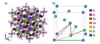
Figure 1: Crystal structure and magnetic exchange paths in Yttrium Iron Garnet (YIG). The conventional unit cell of YIG is represented, with the majority tetrahedral sites marked in green and the minority octahedral sites in blue. Yttrium is depicted as black spheres, and oxygen as red spheres. The first octant of the YIG unit cell is shown, highlighting the two distinct Fe3+ sites: tetrahedral sites in green and octahedral sites in blue Princep2017 .

Note that, for the third nearest neighbours, there are two possibilities of exchange parameters $J_{3a}$ and $J_{3b}$. These two exchange paths are dissimilar and can be distinguished due to the symmetry of the crystal when rotated about the bond vector. The $J_{3a}$ exchange path exhibits a 2-fold symmetry, while the $J_{3b}$ exchange path obey the higher D3 symmetry point group.

For the inelastic neutron scattering calculation, we used the method described in Thz_Spectroscopy , where the double-cross section is given by,

$$\frac{d^{2}\sigma}{d\Omega d\omega}=\left(\frac{\gamma e^{2}}{m_{e}c^{2}}\right)^{2}\left[\frac{g}{2}f(\kappa)\right]^{2}\frac{k_{f}}{k_{i}}\sum_{\alpha,\beta}\left(\delta_{\alpha\beta}-\frac{\kappa_{\alpha}\kappa_{\beta}}{\kappa^{2}}\right)S_{\alpha\beta}(\mathbf{\kappa},\omega)$$ (20)

where $\left(\gamma e^{2}/m_{e}c^{2}\right)^{2}=0.291$ barns is the coupling constant of the neutron to the unpaired electron spins (note the use of cgs units), $g$ is the Landé factor, and $f(\kappa)$ is the magnetic form factor. We also define $\kappa$, which is the scattering vector, such that $\mathbf{\kappa}=k_{f}-k_{i}$, which is the difference in momentum of the incoming and outgoing neutrons. Using the notation $q$ for the momentum of the magnons, we have the relation $\kappa=\mathbf{G}+q$, with $\mathbf{G}$ a reciprocal lattice vector.

We point out that the coupling constant for EELS is two orders of magnitude larger than the neutron’s. This difference is counteracted by the flux of particles in the two experiments. The neutron scattering experiment has a typical flux of $10^{14}$ neutrons cm^-2s^-1 NeutronFlux , which is $10^{5}$ times lower than the typical $10^{19}$ electrons cm^-2s^-1ElectronFlux in an electron microscope, leading to a lower exposition time required by the EELS experiment compared to the INS.

III Results

In figure 2 we compare the experimentally acquired INS given in Princep2017 with the calculated INS using Eq. 20 and the calculated charge-only EELS using Eq. 19. We can see the similarities between the experiment and the calculated spectra for the INS, and compared with the EELS, the same modes are active. Under the discussion made before, both the intensities given in the figures 2-b and 2-c coexist in the EELS spectra. The main differences between the interaction forms, arise from the $q$ dependence and the dependence between the intensity with the angle between the beam orientation and the local magnetic moments’ orientation.

Taking the definition of the spin orientation given in 3, we will keep $\phi=0$ and change the value of $\theta$. In figure 2 we kept the orientation of the magnetic moments aligned with oriented parallel to the axis of $\theta=\pi/2$ and $\phi=0$, while the electron/neutron beam is kept along the z-axis.

In figure 3 we see a strong dependence on the magnetic moments orientation. Here we see that the proposed interaction shows a dependence of the intensity as we change the polar angle $\theta$ of the orientation magnetic moments axis of orientation. In the path $\Gamma-H$ the intensity varies with a cossine relation with the angle between the spin and the beam angles.

(a)

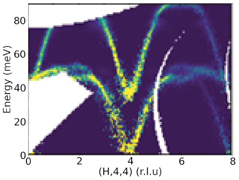
(b) INS

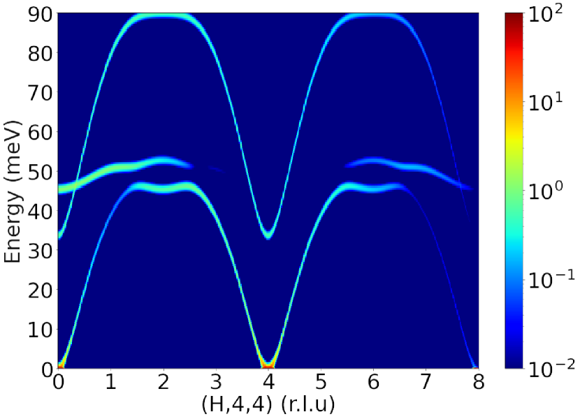
(c) EELS

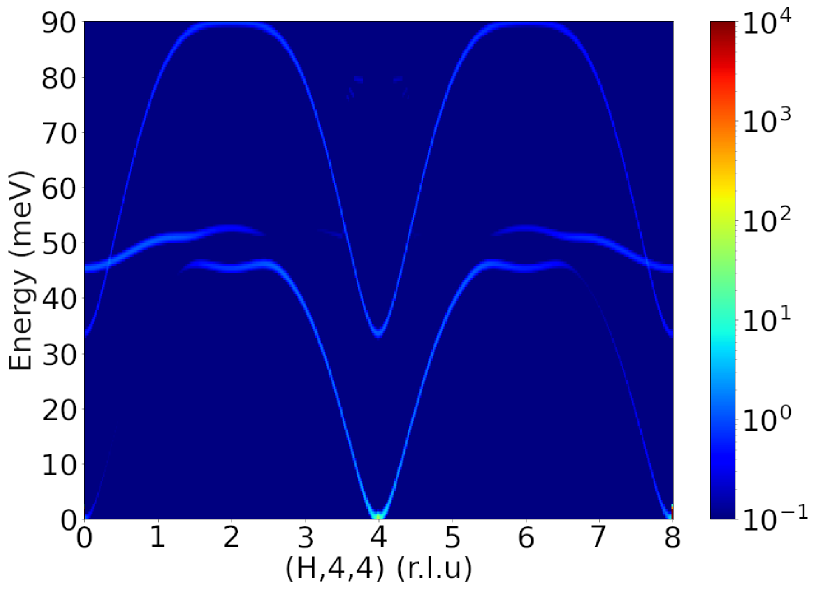
Figure 2: Inelastic scattering by magnons: a) Experimental inelastic neutron scattering Princep2017 , b) theoretical evaluation of inelastic neutron scattering, c) charge-related EELS. All the calculations were performed for a relative angle between the probe’s wave vector and the Nèel vector $\theta=\pi/2$.

(a) $\theta=0$

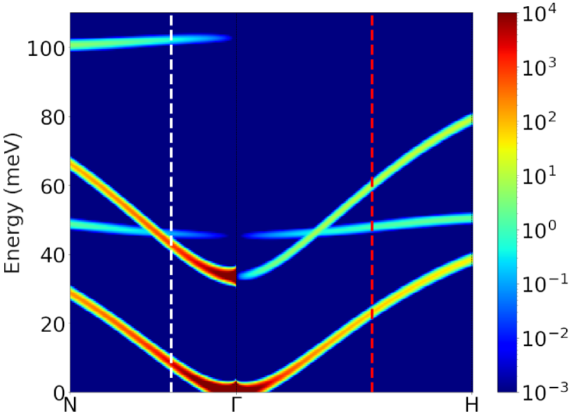
(b) $\theta=3\pi/10$

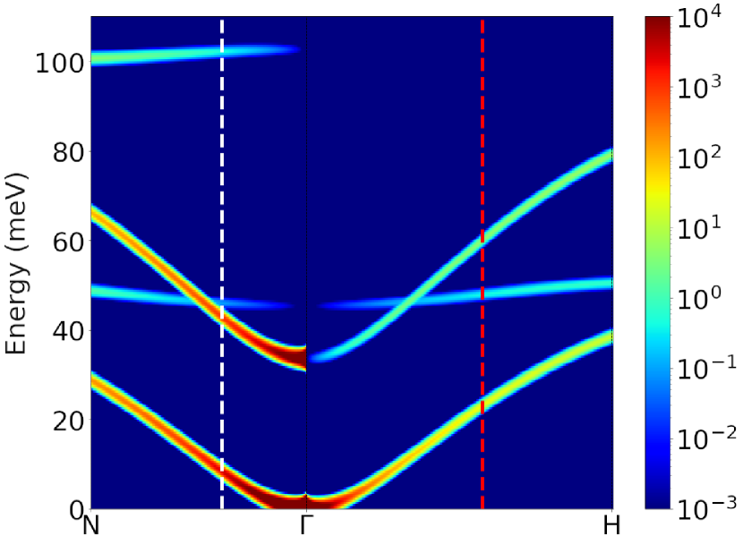
(c) $\theta=\pi/2$

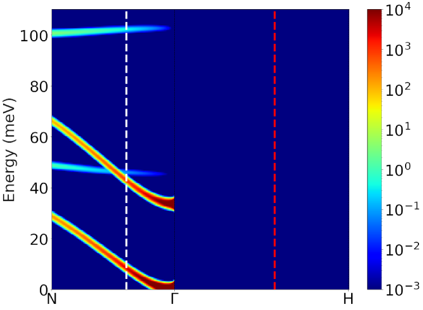
(d) $\theta=7\pi/10$

(e)

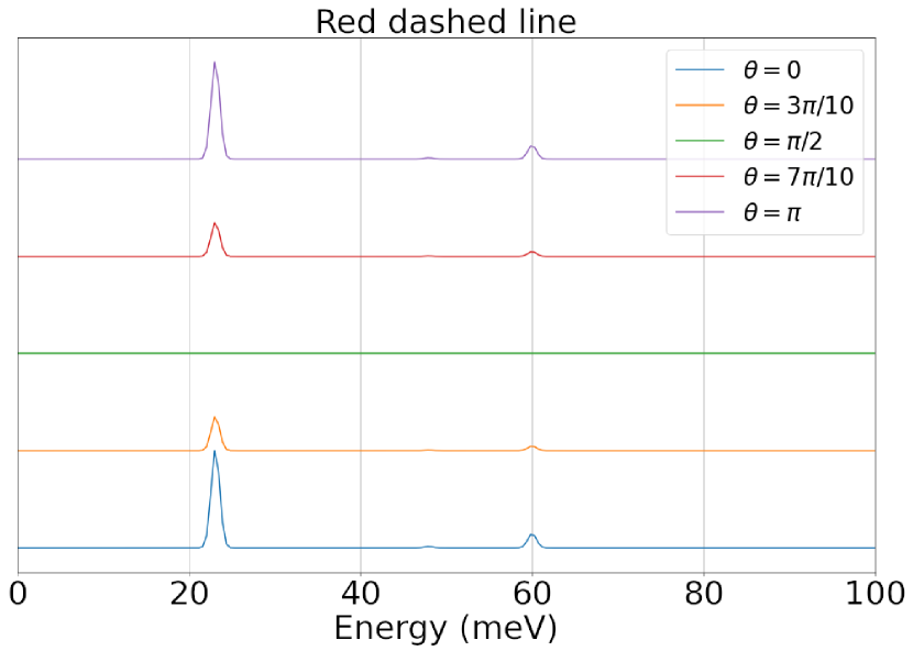
(f)

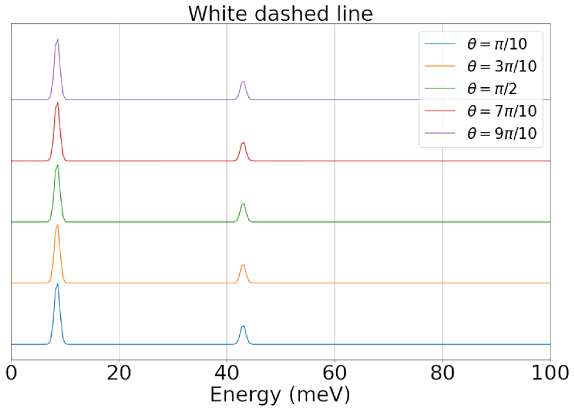
Figure 3: a-d) Charge-related EELS, for varying relative angles $\theta$ between the probe’s wave vector and the Nèel vector. e-f) Angle dependent intensity for a particular point in momentum space, showing a strong angle dependence on the point represented by the red dashed line, but not on the point represented by the white dashed line.

IV Conclusion

The proposed methodology is intended to facilitate the distinction of magnon-related pecks in the EELS experiments when paired with the evaluation of the phonon EEL spectrum. The high spatial resolution united with the magnetic moment orientation sensitive nature of the non-spin polarized EELS spectrum, and given the difference in $q$ dependence, a particular choice of spectra taken from different, but related, scattering vectors can be used to probe local differences in the orientation of the Curie/Neel vector relative to the electron beam momentum.

V Acknowledgement

This project was undertaken on the Viking Cluster, which is a high-performance computing facility provided by the University of York. We are grateful for computational support from the University of York High-Performance Computing service, Viking and the Research Computing team.

References

- [1] Abdulqader Mahmoud, Florin Ciubotaru, Frederic Vanderveken, Andrii V. Chumak, Said Hamdioui, Christoph Adelmann, and Sorin Cotofana. Introduction to spin wave computing. Journal of Applied Physics, 128(16), October 2020.
- [2] Anjan Barman, Gianluca Gubbiotti, S Ladak, A O Adeyeye, M Krawczyk, J Gräfe, C Adelmann, S Cotofana, A Naeemi, V I Vasyuchka, B Hillebrands, S A Nikitov, H Yu, D Grundler, A V Sadovnikov, A A Grachev, S E Sheshukova, J-Y Duquesne, M Marangolo, G Csaba, W Porod, V E Demidov, S Urazhdin, S O Demokritov, E Albisetti, D Petti, R Bertacco, H Schultheiss, V V Kruglyak, V D Poimanov, S Sahoo, J Sinha, H Yang, M Münzenberg, T Moriyama, S Mizukami, P Landeros, R A Gallardo, G Carlotti, J-V Kim, R L Stamps, R E Camley, B Rana, Y Otani, W Yu, T Yu, G E W Bauer, C Back, G S Uhrig, O V Dobrovolskiy, B Budinska, H Qin, S van Dijken, A V Chumak, A Khitun, D E Nikonov, I A Young, B W Zingsem, and M Winklhofer. The 2021 magnonics roadmap. Journal of Physics: Condensed Matter, 33(41):413001, aug 2021.
- [3] Paul S. Keatley, Thomas H. J. Loughran, Euan Hendry, William L. Barnes, Robert J. Hicken, Jeffrey R. Childress, and Jordan A. Katine. A platform for time-resolved scanning Kerr microscopy in the near-field. Review of Scientific Instruments, 88(12):123708, 12 2017.
- [4] Thomas Sebastian, Katrin Schultheiss, Björn Obry, Burkard Hillebrands, and Helmut Schultheiss. Micro-focused brillouin light scattering: imaging spin waves at the nanoscale. Frontiers in Physics, 3, 2015.
- [5] F. S. Hage, D. M. Kepaptsoglou, Q. M. Ramasse, and L. J. Allen. Phonon spectroscopy at atomic resolution. Phys. Rev. Lett., 122:016103, Jan 2019.
- [6] F. S. Hage, G. Radtke, D. M. Kepaptsoglou, M. Lazzeri, and Q. M. Ramasse. Single-atom vibrational spectroscopy in the scanning transmission electron microscope. Science, 367(6482):1124–1127, 2020.
- [7] Eric R Hoglund, De-Liang Bao, Andrew O’Hara, Sara Makarem, Zachary T Piontkowski, Joseph R Matson, Ajay K Yadav, Ryan C Haislmaier, Roman Engel-Herbert, Jon F Ihlefeld, Jayakanth Ravichandran, Ramamoorthy Ramesh, Joshua D Caldwell, Thomas E Beechem, John A Tomko, Jordan A Hachtel, Sokrates T Pantelides, Patrick E Hopkins, and James M Howe. Emergent interface vibrational structure of oxide superlattices. Nature, 601(7894):556–561, 2022.
- [8] J. C. Loudon. Antiferromagnetism in nio observed by transmission electron diffraction. Phys. Rev. Lett., 109:267204, Dec 2012.
- [9] Keenan Lyon, Anders Bergman, Paul Zeiger, Demie Kepaptsoglou, Quentin M. Ramasse, Juan Carlos Idrobo, and Ján Rusz. Theory of magnon diffuse scattering in scanning transmission electron microscopy. Phys. Rev. B, 104:214418, Dec 2021.
- [10] Benjamin Plotkin-Swing, George J. Corbin, Sacha De Carlo, Niklas Dellby, Christoph Hoermann, Matthew V. Hoffman, Tracy C. Lovejoy, Chris E. Meyer, Andreas Mittelberger, Radosav Pantelic, Luca Piazza, and Ondrej L. Krivanek. Hybrid pixel direct detector for electron energy loss spectroscopy. Ultramicroscopy, 217:113067, 2020.
- [11] O.L. Krivanek, N. Dellby, J.A. Hachtel, J.-C. Idrobo, M.T. Hotz, B. Plotkin-Swing, N.J. Bacon, A.L. Bleloch, G.J. Corbin, M.V. Hoffman, C.E. Meyer, and T.C. Lovejoy. Progress in ultrahigh energy resolution eels. Ultramicroscopy, 203:60–67, 2019. 75th Birthday of Christian Colliex, 85th Birthday of Archie Howie, and 75th Birthday of Hannes Lichte / PICO 2019 - Fifth Conference on Frontiers of Aberration Corrected Electron Microscopy.
- [12] B.G. Mendis. Quantum theory of magnon excitation by high energy electron beams. Ultramicroscopy, 239:113548, September 2022.
- [13] Randy S Fishman, Jaime A Fernandez-Baca, and Toomas Rõõm. Spin-Wave Theory and its Applications to Neutron Scattering and THz Spectroscopy. 2053-2571. Morgan and Claypool Publishers, 2018.
- [14] Seamus Beairsto, Maximilien Cazayous, Randy S. Fishman, and Rogério de Sousa. Confined magnons. Phys. Rev. B, 104:134415, Oct 2021.
- [15] Julio A. do Nascimento, Adam Kerrigan, S. A. Cavill, Phil J. Hasnip, Demie Kepaptsoglou, Quentin M. Ramasse, and Vlado K. Lazarov. Confined magnon dispersion in ferromagnetic and antiferromagnetic thin films in a second quantization approach: the case of fe and nio, 2023.
- [16] R. J. Nicholls, F. S. Hage, D. G. McCulloch, Q. M. Ramasse, K. Refson, and J. R. Yates. Theory of momentum-resolved phonon spectroscopy in the electron microscope. Phys. Rev. B, 99:094105, Mar 2019.
- [17] Bruce S. Hudson. Inelastic neutron scattering: A tool in molecular vibrational spectroscopy and a test of ab initio methods. The Journal of Physical Chemistry A, 105(16):3949–3960, 2001.
- [18] Andrew J. Princep, Russell A. Ewings, Simon Ward, Sandor Tóth, Carsten Dubs, Dharmalingam Prabhakaran, and Andrew T. Boothroyd. The full magnon spectrum of yttrium iron garnet. npj Quantum Materials, 2(1), November 2017.
- [19] Stewart F. Parker. Inelastic neutron scattering, instrumentation*. In John C. Lindon, editor, Encyclopedia of Spectroscopy and Spectrometry (Second Edition), pages 1035–1044. Academic Press, Oxford, second edition edition, 2010.
- [20] Martha Ilett, Mark S’ari, Helen Freeman, Zabeada Aslam, Natalia Koniuch, Maryam Afzali, James Cattle, Robert Hooley, Teresa Roncal-Herrero, Sean M. Collins, Nicole Hondow, Andy Brown, and Rik Brydson. Analysis of complex, beam-sensitive materials by transmission electron microscopy and associated techniques. Philosophical Transactions of the Royal Society A: Mathematical, Physical and Engineering Sciences, 378(2186):20190601, October 2020.