Learning Dynamics from Multicellular Graphs with Deep Neural Networks

Abstract

The inference of multicellular self-assembly is the central quest of understanding morphogenesis, including embryos, organoids, tumors, and many others. However, it has been tremendously difficult to identify structural features that can indicate multicellular dynamics. Here we propose to harness the predictive power of graph-based deep neural networks (GNN) to discover important graph features that can predict dynamics. To demonstrate, we apply a physically informed GNN (piGNN) to predict the motility of multicellular collectives from a snapshot of their positions both in experiments and simulations. We demonstrate that piGNN is capable of navigating through complex graph features of multicellular living systems, which otherwise can not be achieved by classical mechanistic models. With increasing amounts of multicellular data, we propose that collaborative efforts can be made to create a multicellular data bank (MDB) from which it is possible to construct a large multicellular graph model (LMGM) for general-purposed predictions of multicellular organization.

1 Introduction

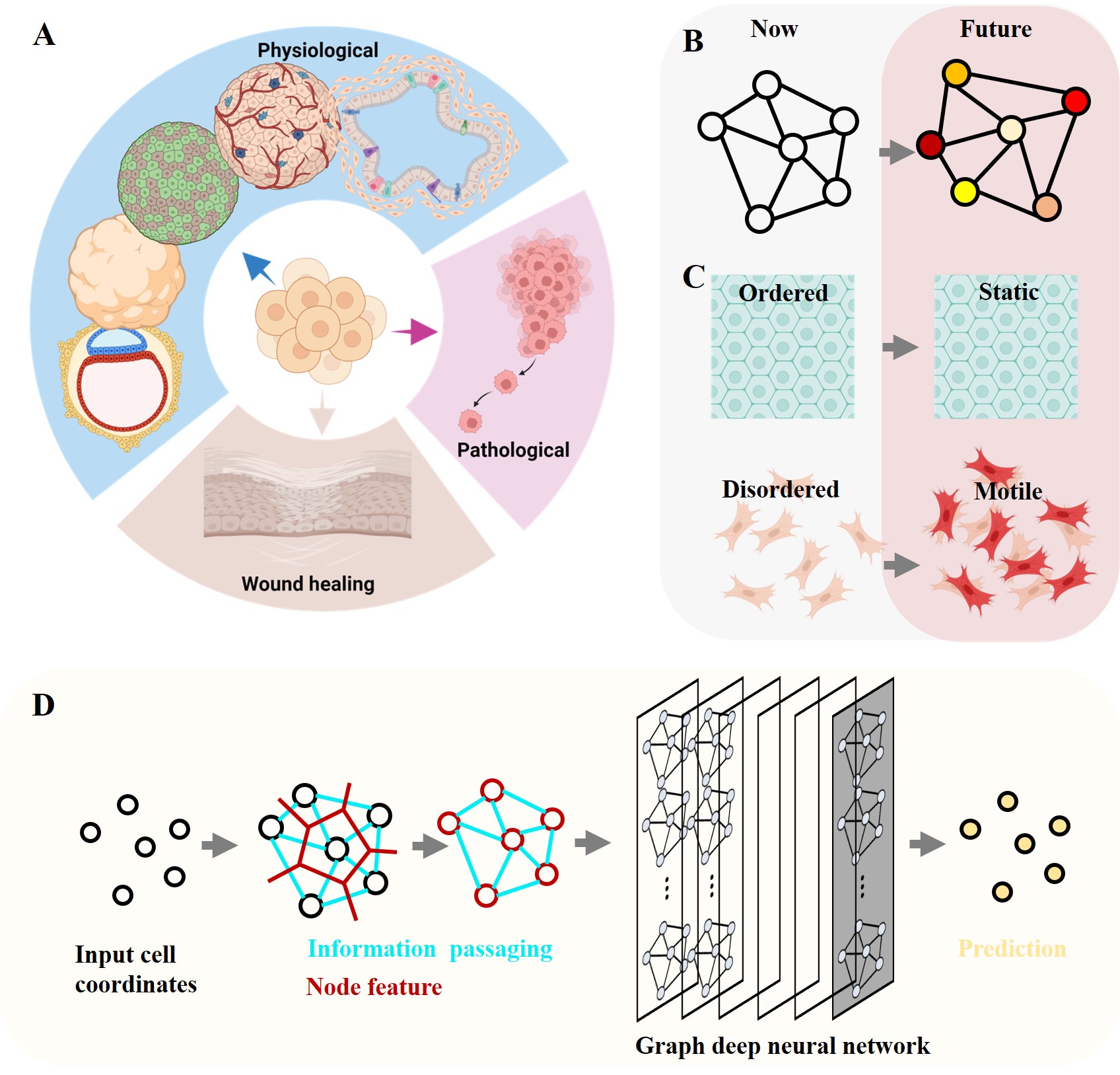
Figure 1: Schematics. (A) Multicellular positioning is the key to morphogenesis, for example (from left to right) embryo, brain, lung, liver and intestinal organoids, pathological processes such as tumors and cancers, as well as wound healing. (B) Multicellular positioning can be abstracted as mapping between current and future multicellular graphs. (C) A qualitative relation between multicellular graphs and dynamics is well known, that more ordered graphs are more static while more disordered graphs are more motile, a glassy behavior that cell monolayers are known to exhibit (Angelini et al., 2011; Bi et al., 2016). (D) piGNN (physically informed graph neural networks). From the input cell coordinates, Voronoi and Delaunay tesselations are performed. The area and perimeter of the Voronoi graphs are taken to be the node embedding, the Delaunay graphs are taken to be the edges for information passaging, and the length of edges are taken to be the edge attribute. (A and C) are created with biorender.com.

The inference of multicellular positioning is critical for our fundamental understanding of morphogenesis during many biological and pathological processes (Fig. 1A), including embryogenesis, vascularization, metastasis, healing, and biofilm formation (Keller, 2013; Xiong et al., 2014; McDole et al., 2018; Kasza et al., 2019; Wang et al., 2020; Atia et al., 2018; Tang et al., 2022; Park et al., 2015; Trepat et al., 2009; Han et al., 2020; Kang et al., 2021; Fuhs et al., 2022; Huang et al., 2022; Jeon et al., 2015; Zervantonakis et al., 2012; Xu et al., 2023; Skinner et al., 2021; Zhang et al., 2021). It has a broad impact on medical and engineering fields such as histology, organoid-on-chip, and 3D bio-printing for drug screening and disease models (Kamm et al., 2018). Despite that modern fluorescent optical microscopy has enabled visualization of the evolution of living multicellular structures in real-time, the principles they follow to self-organize into a complex living structure remain unclear (Keller, 2013; Kamm et al., 2018; Trepat & Sahai, 2018; Karsenti, 2008). While classical mechanistic active-matter models severely rely on the assumptions of symmetries and constitutive relations, data-driven inference methods can potentially bypass some of these biases (Cichos et al., 2020; Brückner & Broedersz, 2023; Brückner et al., 2019; Romeo et al., 2021; Brückner et al., 2021; LaChance et al., 2022; Supekar et al., 2023; Bhaskar et al., 2021; Frishman & Ronceray, 2020).

At the mesoscale, under a microscope, many multicellular living systems, such as embryos, organoids, tumors, and epithelia, are composed of closely packed cells forming cell-cell contact; in systems where cells such as fibroblasts and endothelial cells are embedded inside the extracellular matrices (ECM), they interact through the ECM via biophysical, biomechanical and biochemical cues; among neuron cells, they establish long-ranged information exchange through bioelectrical signals. All these systems can be abstracted as ‘graphs’ consisting of nodes (cells) with multi-modal node embedding (cell identities) and edges (cell-cell interactions) with multi-modal edge attributes (physical, mechanical, chemical, and electrical signals). It was not until recent years that the graph features of multicellular living systems were utilized to predict multicellular dynamics. Similar to glassy colloidal systems where tremendous efforts have also been made to predict dynamics from a snapshot of the system (Bapst et al., 2020; Biroli & Garrahan, 2013), it only becomes more difficult to identify metrics from snapshots that can predict multicellular positioning, given the open and active nature of living cells. Remarkably, research in the past decade has revealed that there indeed exist relations between multicellular graphs and multicellular dynamics, for example, cell shape index, aspect ratio, from the Voronoi graphs (Bi et al., 2016; Atia et al., 2018), and cell alignment, volume and shear order from the Delaunay graphs (Wang et al., 2020; Yang et al., 2021). Recently, it has also been proposed that topological features of Delaunay graphs contain important information that can distinguish living and nonliving materials (Skinner et al., 2022).

Nevertheless, the shortcomings of analytical graph features are still evident. Firstly, these analytical graph features significantly prune the information from the original degree of freedom, while more critical features can exist, and are not necessarily analytical. Secondly, statistics such as average and median are the most popular choices, while they are not necessarily adequate to fully characterize the probability distribution. Thirdly, analytical metrics are often ‘local’, in the sense that longer-ranged higher-order interactions are entirely ignored. Lastly, in more physiologically relevant multicellular systems consisting of cells with multi-modal identities, it will be almost impossible to expand the analytical criteria for cell dynamics from both configurational parameters and multi-modal biological identities. To ultimately make predictions for multicellular organization, it is critical to identify tools that are capable of capturing the comprehensive nonlinear interactions and spatial arrangement, and flexible of concatenating input and output channels for multi-modal biological information.

Recent developments in the graph-based deep neural networks (GNN) (Corso et al., 2020; Kipf & Welling, 2016) provide an opportunity to develop data-driven models of complex systems, especially focused on models that take advantage of known structural features. For instance, some studies have used graph-based modeling to capture complex multiscale materials phenomena in diverse materials ranging from proteins, crystalline materials, to spider webs (Yang & Buehler, 2022; Guo & Buehler, 2022; Lu et al., 2023), including dynamical properties. Other work has focused on dynamical materials phenomena (Buehler, 2022) using attention-based graph models in conjunction with denoising algorithms applied to model dynamic fracture. The key objective of this paper is to explore if and how we can develop a framework for general predictions of the dynamical behavior of multicellular living systems, here focused on graph-based methods that learn the relationship between geometry and movements.

We propose to harness the predictive power of GNN to discover from data the important graph features relating to multicellular dynamics. Graph-based neural networks are excellent options, especially for multicellular systems accounting for information passaging among node embeddings (cell identities) through edge embeddings (cell-cell interactions). Further, we also propose a physically informed GNN for multicellular systems (piGNN) to demonstrate how existing physical knowledge can be used to inform the graph deep neural network to improve its performance (Fig. 1). We demonstrate that a graph is a powerful way to represent multicellular data, and with the help of deep neural networks, it is possible to construct a large multicellular graph model (LMGM) for general predictions of morphogenesis.

2 Results

Here we apply the proposed graph neural network piGNN (Fig. 1D, see Materials and Methods for details) to predict the multicellular motility in both experiments and simulation, both with changing cell number densities and with constant cell number densities with perturbations on cell-cell interaction and self-propelling velocity. With a series ablation of input information, we show that the relative positioning among the cells is critical for predicting collective cell dynamics, and informing GNN with prior physical information can enhance its performance.

2.1 Learning multicellular dynamics from a graph snapshot

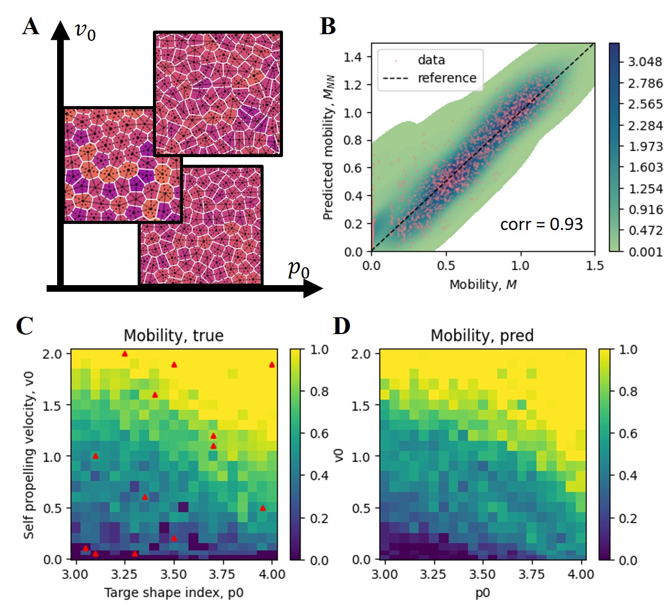
Figure 2: piGNN learns the implicit relation between graph and motility from partial information from simulated cell monolayers. (A) Representative input graphs. The color on the Voronoi polygons indicates the area. (B) Prediction vs. ground truth. The color map indicates probability density. (C) mobility landscape. Red markers, a small portion of the macroscopic state points ($N_{s}=13$) are provided for training. (D) Predicted mobility landscape.

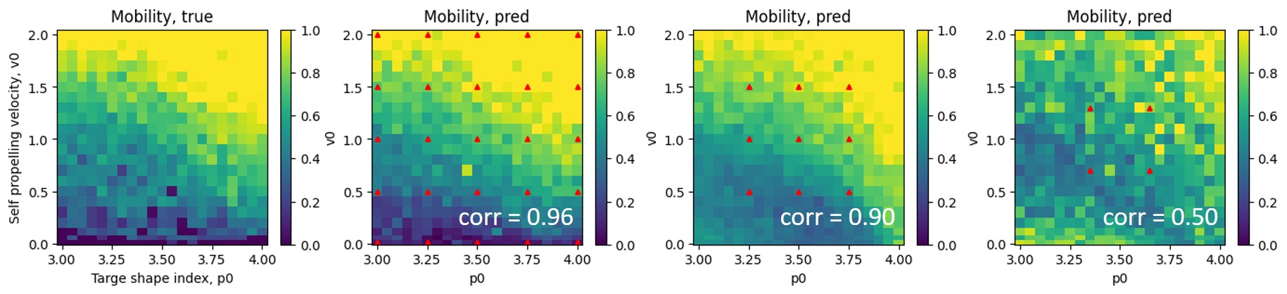
Figure S1: Dependency on the number of states of the train set (with piGNN). Red markers, state points provided for training.

We first demonstrate the power of deep neural networks in predicting multicellular dynamics with a systematical variation of cell-cell interaction and self-propelling strength at a constant cell number density. We seek to learn and predict cell mobility $M$ from static graphs consisting of nodes (cell positions) and edges (cell-cell contact). To do so, we use a dataset of simulated epithelial monolayers, containing steady-state 2D cell positions (Bi et al., 2016; Yang et al., 2021). Each simulation in the dataset is performed with different target shape index $p_{0}$ and self-propelling velocity $v_{0}$, and the dataset consists of 462 distinct sets of configurations with different $(p_{0},v_{0})$ (Fig. 2C). piGNN is trained on a small number of state points, and is used to make predictions for the whole dataset. Here, the graph neural network functions as a universal function approximator to interpolate from the graphs to the mobility. With 4 state points provided, the graph model achieves a correlation of 0.5, while 9 state points for training can increase the correlation to 0.9, and 25 state points is sufficient to increase the correlation to 0.96 (Fig. S1). Surprisingly, the graph neural network is capable of learning the relation from only 13 randomly selected state points (Fig. 2C). It achieves a high accuracy and recovers the mobility landscape (Fig. 2B&D).

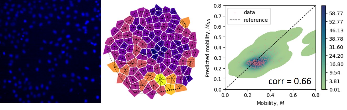
Figure 3: Predicting cell motility in experimental dataset. (Left) A representative snapshot of the dataset. Nuclei were stained (blue). (Middle) A representative input graph. The color of the Voronoi polygons indicates the area. The dashed lines indicate the edges generated from Delaunay triangulation. (Right) mobility prediction $M_{NN}$ vs ground truth $M$ in the validation set. The color map indicates probability density.

To test the same framework in experiments, we create the experimental dataset by culturing MCF-10A cells on collagen-coated substrate and imaging cell positions over time (the dataset consists of 797 train graphs and 352 validation graphs, see Materials and Methods for details regarding preparing the graph from raw videos). The piGNN is trained on the dataset (See Materials and Methods for details regarding the neural network architecture and the training procedure), and a reasonable prediction can be achieved (Fig. 3, bottom). Note that the train and validation sets are from entirely different locations, and none of the frames in the validation set come from the same videos as the train set.

To summarize, the predictions achieved by piGNN indicate that static multicellular configurations contain critical features that can be utilized to predict multicellular dynamics. While it has been an extremely difficult task for classical mechanistic models to regress from static graphs toward dynamics, graph-based deep neural networks provide a model-free solution.

2.2 What information is important?

	Type of information
Model	nonlinear relation	relative positions	physical info.
piGNN	✓	✓	✓
GNN	✓	✓
MLP	✓		✓
AS			✓

Table 1: Four typical models are compared, with different combinations of information provided. piGNN, physically informed graph neural nets. GNN, graph neural nets provided with constant node embedding. MLP, fully connected multi-layer perception with shape index input. AS, analytical statistics. Here we use the median of the cell shape index.

Intuitively, piGNN achieves good performance with a minimal amount of data because it is capable of considering relative positional information in a nonlinear way, as well as because it is physically informed with geometrical quantities that are known to be important in predicting multicellular dynamics. To understand what information is indeed important for its excellent performance, we perform a series of training tasks with the ablation of input information with the simulation dataset (Table 1, Fig. 4).

We first ablate the physical information by providing only constant node embedding into the GNN (GNN, Table 1). While the piGNN achieves a mean squared error ($MSE$) $\sim 0.01$ of and $corr\sim 0.96$, this ablation impairs its performance, raising $MSE$ to $\sim 0.05$, and decreasing $corr$ to $\sim 0.77$ (Fig. 4B&C). On the other hand, we ablate the information of relative position by using fully connected multi-layer perception (MLP, Table 1). Similarly, this ablation increases $MSE$ to $\sim 0.05$ and decreases $corr$ to $\sim 0.77$ (Fig. 4B&C). The impaired performance of both the regular GNN and the MLP models are comparable to a linear regression model using the analytical feature (AS, Table 1), i.e. the median of the SI (shape index, calculated as $perimeter/\sqrt{area}$ for each Voronoi polygon) (Fig. 4B&C). Remarkably, while either relative position or physical information is not adequate, providing both types of information into piGNN can achieve an excellent performance (Fig. 4).

This ablation experiment suggests that cell locations and their spatial interactions are critical to predicting multicellular dynamics. Beyond single-cell morphology, it proves that there exist complex features of the multicellular graphs that are useful for predicting multicellular dynamics. While classical mechanistic models heavily rely on intuitions and assumptions to distill a handful of structural metrics, graph-based deep neural networks are capable of bypassing these assumptions and discovering hidden relations from information of the whole graph.

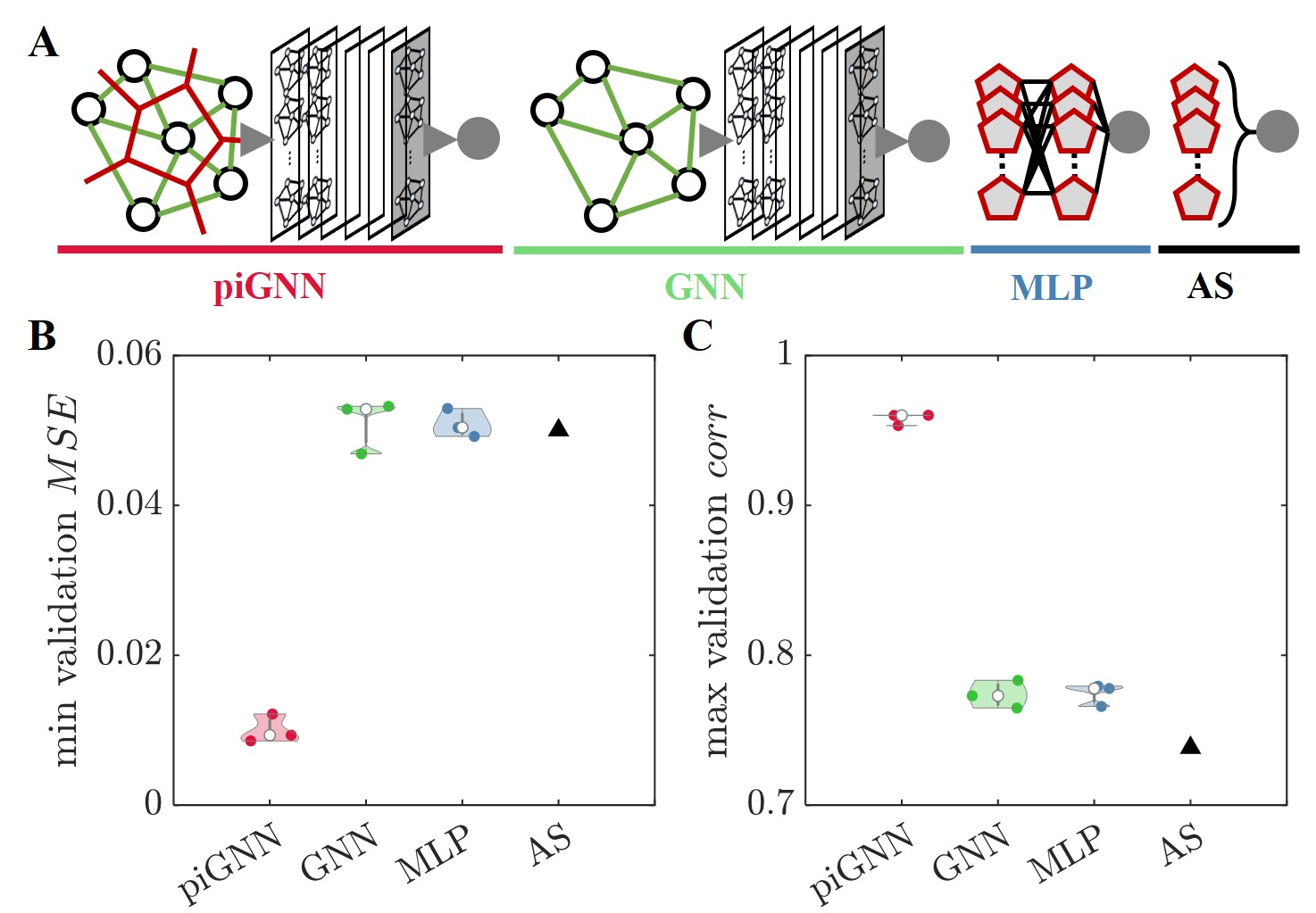
Figure 4: Comparing the performance of different models. (A) Different model architectures. piGNN, graph neural networks informed with physical information. GNN, graph neural networks with constant node embedding. MLP, fully connected multi-layer perception. AS, analytical statistics (i.e. median of shape index). We further compare the performance of different models with (B) min $MSE$ (C) max $corr$ on the validation set, where min and max are taken in one training across all epochs. The experiment with each model is performed 3 times, initialized with different random seed numbers. Training is performed on the simulation dataset with $N_{s}=25$ state points.

To further understand how graph-based learning might have gained additional insights into multicellular dynamics, we can consider a multi-body system whose dynamic equation is

$$\frac{d\mathbf{x}_{i}}{dt}=\mu\mathbf{F({\{\mathbf{x}_{i}}\})}+v_{0}\bm{\zeta},$$ (1)

where $\mathbf{x}_{i}$ is the Cartesian coordinates, $t$ is time, $\mathbf{F}$ is the interaction force that could in principle depend on all the degrees of freedom $\mathbf{x}_{i}$, $\bm{\zeta}$ is a unit noise term, $\mu$ is a coefficient and $v_{0}$ is the self-propelling velocity, $i=1,2,...N$ is the index of the $i$th cell. While this is still an oversimplification of multicellular living systems, we can gain some insight into how learning might benefit from a graph-based construction.

Here the multi-body force $\mathbf{F}(\{\mathbf{x}_{i}\})$ is the unknown, and we are given a number of observations of $\{\mathbf{x}_{i}\}$. The task of either mechanistic models or deep learning models can be regarded as inferring either an analytical approximation or a neural network approximation for $\mathbf{F}(\{\mathbf{x}_{i}\})$, which is highly complex in a multicellular living system. A common choice might be first to expand $\mathbf{F}(\{\mathbf{x}_{i}\})$ as a sum of multi-body interaction terms (Brückner & Broedersz, 2023):

$$\mathbf{F}(\{\mathbf{x}_{i}\}) \simeq\sum_{i}\mathbf{F}^{(1)}(\mathbf{x}_{i})$$ (2)

$$+\sum_{i}\sum_{j}\mathbf{F}^{(2)}(\mathbf{x}_{i},\mathbf{x}_{j})$$

$$+\sum_{i}\sum_{j}\sum_{k}\mathbf{F}^{(3)}(\mathbf{x}_{i},\mathbf{x}_{j},\mathbf{x}_{k})+...$$

In recent studies, several inference models have been constructed for active matter under this decomposition and a focus has been on estimating the two-body term $\sum_{i}\sum_{j}\mathbf{F}^{(2)}(\mathbf{x}_{i},\mathbf{x}_{j})$. The underlining assumption is that $|\mathbf{F}^{(n>2)}|\ll|\mathbf{F}^{(2)}|$. This assumption is generally true in classical systems, but in living systems, such interactions are multi-body in nature, meaning that $|\mathbf{F}^{(n>2)}|$ is not necessarily negligible compared to $|\mathbf{F}^{(2)}|$, but rather depends on the relative connections (edges) across many cells. Graph-based learning provides an alternative option through estimating $\mathbf{F}$ instead from graphs:

$$\mathbf{F}(\{\mathbf{x}_{i}\}) \simeq\mathbf{F}^{(0)}(g^{(0)})$$ (3)

$$+\sum_{n}\mathbf{F}^{(n)}(g^{(n)}),$$

where $g$ are graphs. In piGNN, a specific graph is chosen as the primary graph $g^{(0)}$, and learning is entirely based on $g^{(0)}$ (See Materials and Methods), while other graph structures can be further explored. Notably, in more realistic situations where $\mathbf{F}$ is not only a function of cell positions $\{\mathbf{x}_{i}\}$, but also a function of other multi-omics $\{\mathbf{o}_{i}\}$, the proposed framework is flexible enough to concatenate the information together as input embedding.

3 Discussions

With the help of graph-based deep neural networks, we propose that a collaborative effort can be made to create a multicellular data bank (MDB) from which it will be possible to construct a large multicellular graph model (LMGM) for general-purposed predictions of multicellular positioning (Fig. 5).

Efficient data representation and multicellular data bank (MDB). This century witnessed the fast growth of multicellular data for a variety of tissues and organs, yet it has been difficult to identify a universal model (either theoretical or computational) that can be predictive of the organization and dynamics of multicellular systems. Remarkably, it is still unclear what is a standard representation of multicellular data. Learning from data, the excellent performance of graph-based deep neural networks proves that multicellular graphs contain important hidden information that determines multicellular dynamics. On the other hand, from a technical aspect, the raw multicellular data are high-dimensional, typically z-stacked (3D), time-lapse (dynamical), and multi-channel (multi-omics). The data size for a single biological sample at acceptable resolution can typically be on the order of 1-10 gigabytes. A large-scale deep neural network based on video representation greatly exceeds the current data process, transfer, and storage capacity. For the purpose of LMGM, it is required to have a standard efficient data representation that can condense the data while retaining the important information. The graph-based representation proposed in this study provides a possible solution. We note that while the edge and edge attributes in the current analysis are ‘artificial’ given the data we have at hand, important biological edges such as cell junctions and even long-ranged neurological connections can be easily included in the framework. Nevertheless, the positions of the cell nuclei can be used as the ‘backbone’ of multicellular data, to which multi-omics data can be attached. While ideally dynamic multi-omic experiments can be performed in one round with multi-channel live staining, practically multiple experiments performed on one biological sample typically require multiple runs under multiple microscopes. Coordinate alignment can be first achieved using the coordinates of the cell nuclei (Fig. 5). With the graph-based data representation and graph-based deep neural network, the pipeline proposed in this work, along with the accompanying implementations shared via open source code, provide a paradigm for systematically organizing multicellular data into a multicellular data bank, and further condensed into graph-based deep neural networks for general predictions.

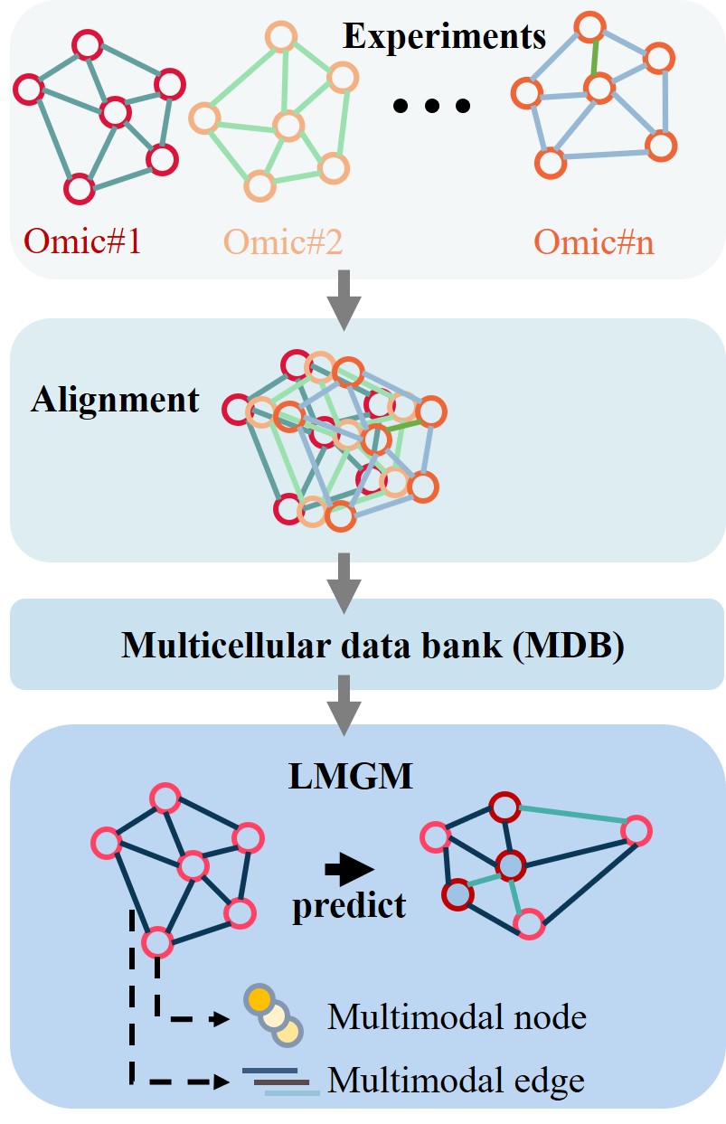
Figure 5: A blueprint for a unified large multicellular graph model (LMGM).

Large multicellular graph model (LMGM). At a smaller length scale, deep neural nets (e.g. AlphaFold) have successfully uncovered the folded structure of ‘graphs’ of proteins (Jumper et al., 2021).

Is it possible to train a large model for general predictions of multicellular organization?

The graph-based deep neural networks provide an excellent option that is capable of concatenating multi-omic biological inputs and outputs in an extremely flexible way. It is therefore possible to further include genetics, proteomics, and other in situ multi-omic data as node embeddings, while cell-cell junctions, mechanical interactions, and other interactions can be treated as edge-embedding; these multi-omics graphs can then be provided to a graph neural network for prediction of missing/future features on these multicellular graphs. Hence, we believe that this framework holds great potential for organizing fast-increasing multicellular data, and provides a possible solution to construct LMGM.

4 Materials and Methods

4.1 Problem Setup

The overall pipeline is shown in Fig. 1, and some details are discussed here.

Graph inputs.— While we focused on 2D systems in this paper for easier demonstration, the framework can be easily extended to 3D. In both the experiment and simulation datasets, the raw input data are multiple sets of cell coordinates over time

$$(x_{i,t},y_{i,t}),\,i=1,2,...,N(t),\,\mathrm{and}\quad t=1,2,...,T\,,$$ (4)

where $x_{i,t}$ and $y_{i,t}$ are Cartesian coordinates of the $i$th cell in the frame $t$, $N(t)$ is the total number of cells at frame $t$, and $T$ is the total number of frames.

Each input graph $g$ is defined through a set of nodes and a set of edges, as

$$g=\{\mathcal{N};\mathcal{E}\}\,,$$ (5)

where $\mathcal{N}$ is a set of nodes containing multi-modal node embedding, and $\mathcal{E}$ is a set of edges containing multi-modal edge attributes.

In each frame, Delaunay triangulation and Voronoi tesselation are performed. Unless otherwise noted, the cell positions are used as nodes, the area $a$ and perimeter $p$ of the Voronoi cells are used as node embeddings, the Delaunay edges $\mathbf{e}$ are used as edges and the length of the edges are used as the edge attribute $l$.

$$\mathcal{N} =\{(a,p)\}\,,$$ (6)

$$\mathcal{E} =\{l\}.$$

In the case that multi-omics data are collected, more information can be concatenated into $\mathcal{N}$ and $\mathcal{E}$.

mobility outputs.—The cell mobility $M$ can be calculated by comparing the $t$ frame with the $t+lag$ frame in its future time. The mobility is

$$M=\frac{1}{C}\left(\sum_{i}^{N(t)}\left[(x_{i,t+lag}-x_{i,t})^{2}+(y_{i,t+lag}-y_{i,t})^{2}\right]\right)^{1/2}$$ (7)

where $C$ is a constant for the whole dataset to normalize such that $M$ is distributed around 1.

Neural network prediction.—The neural network $\mathcal{G}$ is a function that maps $g$ towards the prediction $M_{NN}$, as

$$M_{NN}=\mathcal{G}(g).$$ (8)

Loss function.—Mean squared error ($MSE$) is used throughout the paper.

Evaluating performance by Pearson correlation.—Throughout this study, the Pearson correlation factor $corr$ is used to evaluate and compare the performance of the models. The Pearson correlation factor $corr$ between the truth and prediction vectors is calculated as

$$corr=\frac{\sum(M_{NN}-\bar{M}_{NN})(M-\bar{M})}{\sqrt{\sum(M_{NN}-\bar{M}_{NN})^{2}\sum(M-\bar{M})^{2}}}\,,$$ (9)

where the summation is taken over the whole validation set.

4.2 Experiments

Datasets.—We used the non-tumorigenic human breast epithelial cell line MCF-10A to create the experimental dataset. The cells were stained (SPY650-DNA) for fluorescent imaging of the cell nuclei. The cells were seeded at 10 different cell number densities (4 locations at each density, 3 for training and 1 for validation): 5,000 to 50,000 in steps of 5000 cells per well of 96-well plates. The substrates are collagen-coated (Serva, cat. No. 47254.01). The cells were allowed to rest overnight in the incubator to fully attach to the substrate. A total of 40 videos were recorded simultaneously every 3 minutes for 16 hours ( 300 frames). Imaging was performed using a WiScan Hermes High Content Imaging System (Idea Biomedical). Cell tracking was performed using TrackMate in ImageJ (Ershov et al., 2022). Delaunay triangulation and Voronoi tesselation were performed using scipy.spatial.delaunay and scipy.spatial.voronoi. We calculated the cell mobility $M$ by comparing the $t$ frame with the $t+lag$ frame in its future time with Eq. 7, with $lag=5$. A total of 5 frames (frames 50, 100, 150, 200, 250) are selected to construct the dataset. For each frame, we first selected the middle region of the field of view (0.25-0.75 the range of both axes), and picked 1 from every 50 cells as the center node of the graph; Then we selected all the cells within 100 pixel distance to the center node to construct the input graphs (Fig. 3, middle). In total, the train set consists of 797 graphs and the validation set consists of 352 graphs.

The simulation dataset was created with Self-Propelled Voronoi simulations (Bi et al., 2016; Yang et al., 2021). The simulation contains two important parameters, the target shape index $p_{0}$ which quantifies the relative strength of cell-cell interaction, and the self-propelling velocity $v_{0}$. The simulation was performed with $N=400$ cells. For each state point defined by $(p_{0},v_{0})$, 4000 frames of steady state cell coordinates were generated. In total, the dataset consists of 462 distinct state points, from which we subsampled 4 frames per state point for our task, resulting in a dataset consisting of 4*462 graphs. Delaunay triangulation and Voronoi tesselation were performed using scipy.spatial.delaunay and scipy.spatial.voronoi. To de-drift the raw data, instead of comparing cell positions at two frames, we took the variance of its position within a time window (assigned to be 10 frames here), thus $M=\frac{1}{C}\left(\sum_{i=1}^{N}\sum_{t}\left[(x_{i,t}-\bar{x}_{i})^{2}+(y_{i,t}-\bar{y}_{i})^{2}\right]\right)^{1/2}$, where $\bar{x_{i}}$ and $\bar{y_{i}}$ are the mean coordinates of cell $i$ within the frame window.

Training GNN.—The graph neural net was implemented with PyTorch Geometric (Fey & Lenssen, 2019). In a few closely related fields, it has been shown that GNN models are capable of uncovering these hidden relations in glassy systems (Bapst et al., 2020), as well as making predictions for graphs such as atomic structures, proteins, and spider-web structures (Yang & Buehler, 2022; Guo & Buehler, 2022; Lu et al., 2023). Here, the Permutation-equivariant Node Aggregation (PNA) layer was employed (Corso et al., 2020). We use [sum, mean, std, max, mean] aggregators, along with [identity, amplification, attenuation] scalers. Unless otherwise specified, the network consists of 5 layers with 15 channels and 3 towers; ReLU activation function was used and batch norm layers were applied after each PNA layer; global mean pooling and another linear layer were applied at the end of all the PNA layers to transform to the output dimension. In training the GNN with constant node embedding in Fig. 4, we replace the node embedding with 1. AdamW with learning rate 5e-4 and weight decay 1e-8 is used. The model was trained for 1000 epochs. All the machine learning experiments were performed on Google Colab with an NVIDIA T4 GPU.

Author contribution

H.Y., M.B., and M.G. conceptualized this study. H.Y. performed this study. H.Y., L.Y., and M.B. wrote the machine learning algorithm. F.M., C.L., and M.A.O. collected the experimental cell monolayer data, and S.H. performed cell tracking. H.Y., M.B., and M.G. wrote the paper.

Data availability

The machine-learning algorithm will be available on a GitHub repository. Trained model weights will be available on Hugging Face.

Supplemental Materials

layers	channels	max $corr$
3	9	0.95
4	9	0.96
5	15	0.96
9	15	0.95
9	36	0.94
20	36	0.81

Table S1: Predicting performance of piGNN with different numbers of layers and channels on the whole simulation dataset, with 25 state points for training. 5 layers and 15 channels are used throughout the paper unless otherwise noted.

$N_{g}$	max $corr$
4	0.956
8	0.957
20	0.966
40	0.962

Table S2: Performance of piGNN with different numbers of graphs per state point $N_{g}$ in the simulation dataset, with 25 state points for training. We use $N_{g}=4$ throughout the paper.

layers	channels	max $corr$
3	9	0.763
4	9	0.778
5	15	0.775
7	15	0.795
7	36	0.778
8	36	0.773
9	36	0.774

Table S3: Predicting performance of GNN with constant node embedding with different numbers of layers and channels on the whole simulation dataset, with 25 state points for training. 5 layers and 15 channels are used in the main text.

layers	channels	max $corr$
8	32	0.774
9	32	0.777
10	32	0.774
16	128	0.778
16	400	0.776

Table S4: Predicting performance of MLP with different numbers of layers and channels on the whole simulation dataset, with 25 state points for training. 16 layers and 128 channels are used in the main text.

References

- Angelini et al. (2011) Angelini, T. E., Hannezo, E., Trepat, X., Marquez, M., Fredberg, J. J., and Weitz, D. A. Glass-like dynamics of collective cell migration. Proceedings of the National Academy of Sciences, 108(12):4714–4719, 2011.
- Atia et al. (2018) Atia, L., Bi, D., Sharma, Y., Mitchel, J. A., Gweon, B., A. Koehler, S., DeCamp, S. J., Lan, B., Kim, J. H., Hirsch, R., et al. Geometric constraints during epithelial jamming. Nature physics, 14(6):613–620, 2018.
- Bapst et al. (2020) Bapst, V., Keck, T., Grabska-Barwińska, A., Donner, C., Cubuk, E. D., Schoenholz, S. S., Obika, A., Nelson, A. W., Back, T., Hassabis, D., et al. Unveiling the predictive power of static structure in glassy systems. Nature Physics, 16(4):448–454, 2020.
- Bhaskar et al. (2021) Bhaskar, D., Zhang, W. Y., and Wong, I. Y. Topological data analysis of collective and individual epithelial cells using persistent homology of loops. Soft matter, 17(17):4653–4664, 2021.
- Bi et al. (2016) Bi, D., Yang, X., Marchetti, M. C., and Manning, M. L. Motility-driven glass and jamming transitions in biological tissues. Physical Review X, 6(2):021011, 2016.
- Biroli & Garrahan (2013) Biroli, G. and Garrahan, J. P. Perspective: The glass transition. The Journal of chemical physics, 138(12), 2013.
- Brückner & Broedersz (2023) Brückner, D. B. and Broedersz, C. P. Learning dynamical models of single and collective cell migration: a review. arXiv preprint arXiv:2309.00545, 2023.
- Brückner et al. (2019) Brückner, D. B., Fink, A., Schreiber, C., Röttgermann, P. J., Rädler, J. O., and Broedersz, C. P. Stochastic nonlinear dynamics of confined cell migration in two-state systems. Nature Physics, 15(6):595–601, 2019.
- Brückner et al. (2021) Brückner, D. B., Arlt, N., Fink, A., Ronceray, P., Rädler, J. O., and Broedersz, C. P. Learning the dynamics of cell–cell interactions in confined cell migration. Proceedings of the National Academy of Sciences, 118(7):e2016602118, 2021.
- Buehler (2022) Buehler, M. J. Modeling atomistic dynamic fracture mechanisms using a progressive transformer diffusion model. Journal of Applied Mechanics, 89(12):121009, 2022.
- Cichos et al. (2020) Cichos, F., Gustavsson, K., Mehlig, B., and Volpe, G. Machine learning for active matter. Nature Machine Intelligence, 2(2):94–103, 2020.
- Corso et al. (2020) Corso, G., Cavalleri, L., Beaini, D., Liò, P., and Veličković, P. Principal neighbourhood aggregation for graph nets. Advances in Neural Information Processing Systems, 33:13260–13271, 2020.
- Ershov et al. (2022) Ershov, D., Phan, M.-S., Pylvänäinen, J. W., Rigaud, S. U., Le Blanc, L., Charles-Orszag, A., Conway, J. R., Laine, R. F., Roy, N. H., Bonazzi, D., et al. Trackmate 7: integrating state-of-the-art segmentation algorithms into tracking pipelines. Nature Methods, 19(7):829–832, 2022.
- Fey & Lenssen (2019) Fey, M. and Lenssen, J. E. Fast graph representation learning with pytorch geometric. arXiv preprint arXiv:1903.02428, 2019.
- Frishman & Ronceray (2020) Frishman, A. and Ronceray, P. Learning force fields from stochastic trajectories. Physical Review X, 10(2):021009, 2020.
- Fuhs et al. (2022) Fuhs, T., Wetzel, F., Fritsch, A. W., Li, X., Stange, R., Pawlizak, S., Kießling, T. R., Morawetz, E., Grosser, S., Sauer, F., et al. Rigid tumours contain soft cancer cells. Nature Physics, 18(12):1510–1519, 2022.
- Guo & Buehler (2022) Guo, K. and Buehler, M. J. Rapid prediction of protein natural frequencies using graph neural networks. Digital Discovery, 1(3):277–285, 2022.
- Han et al. (2020) Han, Y. L., Pegoraro, A. F., Li, H., Li, K., Yuan, Y., Xu, G., Gu, Z., Sun, J., Hao, Y., Gupta, S. K., et al. Cell swelling, softening and invasion in a three-dimensional breast cancer model. Nature physics, 16(1):101–108, 2020.
- Huang et al. (2022) Huang, J., Cochran, J. O., Fielding, S. M., Marchetti, M. C., and Bi, D. Shear-driven solidification and nonlinear elasticity in epithelial tissues. Physical Review Letters, 128(17):178001, 2022.
- Jeon et al. (2015) Jeon, J. S., Bersini, S., Gilardi, M., Dubini, G., Charest, J. L., Moretti, M., and Kamm, R. D. Human 3d vascularized organotypic microfluidic assays to study breast cancer cell extravasation. Proceedings of the National Academy of Sciences, 112(1):214–219, 2015.
- Jumper et al. (2021) Jumper, J., Evans, R., Pritzel, A., Green, T., Figurnov, M., Ronneberger, O., Tunyasuvunakool, K., Bates, R., Žídek, A., Potapenko, A., et al. Highly accurate protein structure prediction with alphafold. Nature, 596(7873):583–589, 2021.
- Kamm et al. (2018) Kamm, R. D., Bashir, R., Arora, N., Dar, R. D., Gillette, M. U., Griffith, L. G., Kemp, M. L., Kinlaw, K., Levin, M., Martin, A. C., et al. Perspective: The promise of multi-cellular engineered living systems. APL bioengineering, 2(4), 2018.
- Kang et al. (2021) Kang, W., Ferruzzi, J., Spatarelu, C.-P., Han, Y. L., Sharma, Y., Koehler, S. A., Mitchel, J. A., Khan, A., Butler, J. P., Roblyer, D., et al. A novel jamming phase diagram links tumor invasion to non-equilibrium phase separation. Iscience, 24(11), 2021.
- Karsenti (2008) Karsenti, E. Self-organization in cell biology: a brief history. Nature reviews Molecular cell biology, 9(3):255–262, 2008.
- Kasza et al. (2019) Kasza, K. E., Supriyatno, S., and Zallen, J. A. Cellular defects resulting from disease-related myosin ii mutations in drosophila. Proceedings of the National Academy of Sciences, 116(44):22205–22211, 2019.
- Keller (2013) Keller, P. J. Imaging morphogenesis: technological advances and biological insights. Science, 340(6137):1234168, 2013.
- Kipf & Welling (2016) Kipf, T. N. and Welling, M. Semi-supervised classification with graph convolutional networks. arXiv preprint arXiv:1609.02907, 2016.
- LaChance et al. (2022) LaChance, J., Suh, K., Clausen, J., and Cohen, D. J. Learning the rules of collective cell migration using deep attention networks. PLoS computational biology, 18(4):e1009293, 2022.
- Lu et al. (2023) Lu, W., Lee, N. A., and Buehler, M. J. Modeling and design of heterogeneous hierarchical bioinspired spider web structures using deep learning and additive manufacturing. Proceedings of the National Academy of Sciences, 120(31):e2305273120, 2023.
- McDole et al. (2018) McDole, K., Guignard, L., Amat, F., Berger, A., Malandain, G., Royer, L. A., Turaga, S. C., Branson, K., and Keller, P. J. In toto imaging and reconstruction of post-implantation mouse development at the single-cell level. Cell, 175(3):859–876, 2018.
- Park et al. (2015) Park, J.-A., Kim, J. H., Bi, D., Mitchel, J. A., Qazvini, N. T., Tantisira, K., Park, C. Y., McGill, M., Kim, S.-H., Gweon, B., et al. Unjamming and cell shape in the asthmatic airway epithelium. Nature materials, 14(10):1040–1048, 2015.
- Romeo et al. (2021) Romeo, N., Hastewell, A., Mietke, A., and Dunkel, J. Learning developmental mode dynamics from single-cell trajectories. Elife, 10:e68679, 2021.
- Skinner et al. (2021) Skinner, D. J., Song, B., Jeckel, H., Jelli, E., Drescher, K., and Dunkel, J. Topological metric detects hidden order in disordered media. Physical Review Letters, 126(4):048101, 2021.
- Skinner et al. (2022) Skinner, D. J., Jeckel, H., Martin, A. C., Drescher, K., and Dunkel, J. Topological packing statistics distinguish living and non-living matter. arXiv preprint arXiv:2209.00703, 2022.
- Supekar et al. (2023) Supekar, R., Song, B., Hastewell, A., Choi, G. P., Mietke, A., and Dunkel, J. Learning hydrodynamic equations for active matter from particle simulations and experiments. Proceedings of the National Academy of Sciences, 120(7):e2206994120, 2023.
- Tang et al. (2022) Tang, W., Das, A., Pegoraro, A. F., Han, Y. L., Huang, J., Roberts, D. A., Yang, H., Fredberg, J. J., Kotton, D. N., Bi, D., et al. Collective curvature sensing and fluidity in three-dimensional multicellular systems. Nature Physics, 18(11):1371–1378, 2022.
- Trepat & Sahai (2018) Trepat, X. and Sahai, E. Mesoscale physical principles of collective cell organization. Nature Physics, 14(7):671–682, 2018.
- Trepat et al. (2009) Trepat, X., Wasserman, M. R., Angelini, T. E., Millet, E., Weitz, D. A., Butler, J. P., and Fredberg, J. J. Physical forces during collective cell migration. Nature physics, 5(6):426–430, 2009.
- Wang et al. (2020) Wang, X., Merkel, M., Sutter, L. B., Erdemci-Tandogan, G., Manning, M. L., and Kasza, K. E. Anisotropy links cell shapes to tissue flow during convergent extension. Proceedings of the National Academy of Sciences, 117(24):13541–13551, 2020.
- Xiong et al. (2014) Xiong, F., Ma, W., Hiscock, T. W., Mosaliganti, K. R., Tentner, A. R., Brakke, K. A., Rannou, N., Gelas, A., Souhait, L., Swinburne, I. A., et al. Interplay of cell shape and division orientation promotes robust morphogenesis of developing epithelia. Cell, 159(2):415–427, 2014.
- Xu et al. (2023) Xu, H., Huo, Y., Zhou, Q., Wang, L. A., Cai, P., Doss, B., Huang, C., and Hsia, K. J. Geometry-mediated bridging drives nonadhesive stripe wound healing. Proceedings of the National Academy of Sciences, 120(18):e2221040120, 2023.
- Yang et al. (2021) Yang, H., Pegoraro, A. F., Han, Y., Tang, W., Abeyaratne, R., Bi, D., and Guo, M. Configurational fingerprints of multicellular living systems. Proceedings of the National Academy of Sciences, 118(44):e2109168118, 2021.
- Yang & Buehler (2022) Yang, Z. and Buehler, M. J. Linking atomic structural defects to mesoscale properties in crystalline solids using graph neural networks. npj Computational Materials, 8(1):198, 2022.
- Zervantonakis et al. (2012) Zervantonakis, I. K., Hughes-Alford, S. K., Charest, J. L., Condeelis, J. S., Gertler, F. B., and Kamm, R. D. Three-dimensional microfluidic model for tumor cell intravasation and endothelial barrier function. Proceedings of the National Academy of Sciences, 109(34):13515–13520, 2012.
- Zhang et al. (2021) Zhang, Q., Li, J., Nijjer, J., Lu, H., Kothari, M., Alert, R., Cohen, T., and Yan, J. Morphogenesis and cell ordering in confined bacterial biofilms. Proceedings of the National Academy of Sciences, 118(31):e2107107118, 2021.