Empirical martingale projections via the adapted Wasserstein distance

Abstract

Given a collection of multidimensional pairs $\{(X_{i},Y_{i}):1\leqslant i\leqslant n\}$, we study the problem of projecting the associated suitably smoothed empirical measure onto the space of martingale couplings (i.e. distributions satisfying $\mathbb{E}[Y|X]=X$) using the adapted Wasserstein distance. We call the resulting distance the smoothed empirical martingale projection distance (SE-MPD), for which we obtain an explicit characterization. We also show that the space of martingale couplings remains invariant under the smoothing operation. We study the asymptotic limit of the SE-MPD, which converges at a parametric rate as the sample size increases if the pairs are either i.i.d. or satisfy appropriate mixing assumptions. Additional finite-sample results are also investigated. Using these results, we introduce a novel consistent martingale coupling hypothesis test, which we apply to test the existence of arbitrage opportunities in recently introduced neural network-based generative models for asset pricing calibration.

1 Introduction

Consider a collection $\{(X_{i},Y_{i}):1\leqslant i\leqslant n\}$ of random pairs with values in $\mathbb{R}^{d}\times\mathbb{R}^{d},\,d\geqslant 1$. We denote the associated empirical measure of this sample by $\mathbb{P}_{n}$. The fundamental goal of this paper is to study the following question:

It is natural to formulate this question as a projection problem. In order to do this we first need to overcome a series of modeling challenges, which we describe in the paragraphs below. Once these are addressed, we give a precise formulation of the projection problem and study it rigorously, including an asymptotic analysis as $n$ increases. Both the modeling and the technical methodology constitute the first portion of the main contributions of this paper. The second portion is driven by applications to statistical learning. In fact, the above question is of fundamental importance from an applied standpoint, because it forms the basis of a new consistent statistical test for martingale pairs. We apply this test in order to verify the no-arbitrage condition in asset pricing models and to test the Markov property.

The first modeling issue that arises is the choice of a projection distance. A natural choice to measure the distance between two distributions is the Wasserstein distance, which in our context is given by

$$\mathcal{W}_{\gamma}(\mathbb{P},\mathbb{Q})^{\gamma}=\inf\,\mathbb{E}[\|X-X^{\prime}\|_{2}^{\gamma}+\|Y-Y^{\prime}\|_{2}^{\gamma}].$$ (1)

Here $\gamma\geqslant 1$, $\mathbb{P},\mathbb{Q}$ are two probability measures on $\mathbb{R}^{d}\times\mathbb{R}^{d}$, $\|\cdot\|_{2}$ is the Euclidean norm on $\mathbb{R}^{d}$ and the infimum is taken over joint distributions of $(X,X^{\prime},Y,Y^{\prime})$ with $(X,Y)\buildrel\mathrm{law}\over{\sim}\mathbb{P}$ and $(X^{\prime},Y^{\prime})\buildrel\mathrm{law}\over{\sim}\mathbb{Q}.$ The Wasserstein distance has gained popularity in recent years because of its versatility in a wide range of machine learning tasks; we refer to the monograph [peyre2019computational] and the references therein for an overview. Such versatility may be aided by the fact that the Wasserstein distance embeds $\mathbb{R}^{d}\times\mathbb{R}^{d}$ and metrizes the weak convergence topology, see e.g. [villani2009optimal]. In order to focus the discussion of our contributions in the introduction on the main conceptual challenges, we implicitly assume that $\gamma=1$ and do not delve into the integrability assumptions imposed. We will be precise about these important considerations in the statement of our results and the discussion section at the end of this paper.

A key problem that arises when considering the Wasserstein distance is that the conditional expectation is not a continuous function in the weak topology. That is the case even in the setting of simple examples going back to [veraguas2020fundamental], see Section 4.1. For instance, if $X=0$ and $\mathbb{P}(Y=1)=\mathbb{P}(Y=-1)=1/2$, then $(X,Y)$ forms a martingale pair under $\mathbb{P}$ since $\mathbb{E}[Y|X]=X=0$ under $\mathbb{P}$. However, if $\mathbb{Q}(X=\varepsilon,Y=1)=\mathbb{Q}(X=-\varepsilon,Y=-1)=1/2$, then $|\mathbb{E}[Y|X]|=1$ under $\mathbb{Q}$ even though the Wasserstein distance between $\mathbb{Q}$ and $\mathbb{P}$ is less than $\varepsilon$. In particular, it is possible to approximate models that describe martingale pairs by a sequence of probability measures for which the martingale property fails to hold by a strictly positive gap uniformly along the sequence. For this reason, we consider an enhancement to the Wasserstein distance which addresses these types of issues.

This enhancement is called the adapted Wasserstein distance $\mathcal{AW}_{\gamma}$ and has been studied precisely to deal with situations of this type. Instead of considering all joint distributions of $(X,X^{\prime},Y,Y^{\prime})$ preserving the marginal laws $\mathbb{P},\mathbb{Q}$ in (1), $\mathcal{AW}_{\gamma}$ only considers those, for which additionally the probability distribution $\text{Law}(Y,Y^{\prime}|X,X)$ on $\mathbb{R}^{d}\times\mathbb{R}^{d}$ has marginals $\text{Law}(Y|X)$ and $\text{Law}(Y^{\prime}|X^{\prime})$; joint distributions of this type are called adapted or bi-causal (see Definition 1 below). We refer to [backhoff2020adapted] for a well-written introduction and summary of contributions to the theory of adapted distances, with historical references and comparisons; an incomplete list is given by [aldous1981weak, hoover1984adapted, ruschendorf1985wasserstein, hellwig1996sequential, bion2019wasserstein, lassalle2013causal] and [pflug2010version, pflug2012distance, backhoff2020adapted, acciaio2020causal, backhoff2020all, veraguas2020fundamental]. In particular, under the adapted Wasserstein distance, martingale pairs can only be approximated by probability measures that are close to martingale couplings themselves. As a consequence, the discontinuity issue brought up earlier cannot occur. In fact, the adapted Wasserstein distance induces the coarsest topology that addresses this discontinuity, see [backhoff2020all]. This motivates considering the projection distance to the space of martingale pairs using the adapted distance. However, computing this distance is a highly non-trivial task because the bi-causal constraints mentioned above are defined in terms of infinitely many conditional distribution constraints, and the space of martingale pairs is also defined in terms of infinitely many constraints. One of the main contributions of this work is to provide a closed-form expression for this projection distance in great generality.

The next modeling issue that we consider is the fact that the empirical measure $\mathbb{P}_{n}$ will typically appear far from being a martingale pair, simply because it encodes an empirical sample – note that $Y$ given $X$ under $\mathbb{P}_{n}$ is almost surely deterministic if the samples are drawn i.i.d. from a continuous distribution $\mathbb{P}_{0}$. This issue, as we shall show, is resolved by introducing a smoothing technique. In particular, we consider the law of $(X+\xi,Y+\xi)$, where $\xi$ has a suitable density and is independent of $(X,Y)$. We identify a family of densities for $\xi$ that does not change the nature of the problem. Precisely, we show a result of independent interest: if the characteristic function (i.e. the Fourier transform) of $\xi$ has no zeros in $\mathbb{R}^{d}$ (e.g. if $\xi$ is standard Gaussian) and all random variables involved have finite variance, then $(X,Y)$ forms a martingale pair if and only if $(X+\xi,Y+\xi)$ forms a martingale pair. Therefore, by projecting a smoothed version of $\mathbb{P}_{n}$ using $\mathcal{AW}_{\gamma}$, we do not fundamentally change the nature of the estimation task.

Once these modeling issues have been addressed, we turn to the study of a precise mathematical formulation of our problem based on the smoothed empirical martingale projection distance (SE-MPD): we minimize the adapted Wasserstein distance between the smoothed empirical measure and any martingale pair. We then answer the following technical questions:

• What is the rate of convergence of the SE-MPD if the pairs $\{(X_{i},Y_{i}):1\leqslant i\leqslant n\}$ are i.i.d. samples from a distribution $\mathbb{P}_{0}$ or satisfy some mixing conditions? Does it converge at a parametric rate?

• Can we compute the asymptotic statistics?

• Can we use this projection approach to develop a hypothesis test for martingale pairs? How can we study the power of this projection test?

In this paper, we provide affirmative answers to all of these questions under suitable integrability conditions. In particular, in Theorem 5 (and Theorem 4 for the mixing case), we show that the SE-MPD converges at the parametric rate $O(n^{-1/2})$. Moreover, we characterize the asymptotic limit distribution in terms of the integral of a powered norm of an $\mathbb{R}^{d}$-valued Gaussian random field.

As expected in results that involve kernel smoothing, the asymptotic distribution of the SE-MPD depends on the choice of the kernel’s bandwidth $\sigma$. As we noticed earlier, the empirical distribution $\mathbb{P}_{n}$ is far from being a martingale pair if $\sigma=0$, so it is interesting to ponder the role of the bandwidth parameter. In this paper, we give at least one insight into this issue and consider the asymptotic distribution of the SE-MPD for the case $\sigma\to\infty$. Intuitively, one would expect that the distribution should degenerate to zero, as the smoothing procedure adds a “big (constant) martingale” $(\xi,\xi)$ to the pair $(X,Y)$. Somewhat surprisingly, we show that this is not the case if $\mathbb{P}_{0}(X=Y)<1$. In other words, the smoothing effect does not seem to artificially hide that $\mathbb{P}_{n}$ appears to be within $O(n^{-1/2})$ distance from the space of martingale pairs. On the contrary, it turns out that the SE-MPD offers a natural way to characterize the non-martingality of a law $\mathbb{P}_{0}$. If $\xi$ is Gaussian for example, we can characterize the martingale property in terms of polynomial test functions; that is, $\mathbb{E}[(\mathbb{E}[Y|X]-X)m(X)]=0$ for all polynomials $m$. If this expectation does not vanish for $k$ but it vanishes for $j<k$, this informs the specific choice $n^{1/(2(k+1))}\ll\sigma\ll n^{1/(2k)}$ of the bandwidth parameter, for which the SE-MPD blows up as $n$ increases. Conversely, if only $\mathbb{P}_{n}$ is observed, this phenomenon suggests a natural way for choosing $\sigma$ in order to maximize the power of the test: we select the bandwidth that maximizes the SE-MPD, see Section 2.3.1. A more nuanced question, of course, involves the role of $\sigma$ and even the choice of the smoothing kernel for a fixed sample size $n$. While these are interesting questions and we discuss initial results in this direction in Section 3.2, we leave a complete investigation on these issues for future research.

Our asymptotic statistics of the SE-MPD can be used for non-parametric hypothesis testing of the martingale pair property. This property is related to (although different from) martingale testing, where one often considers a sequence of martingales. We refer to Section 2.3 for a more detailed discussion of this issue. For now let us simply note, that there are various methodologies and approaches to test the martingale property in different settings. For instance, [phillips2014testing] developed a consistent martingale test for a one-dimensional martingale difference sequence. The test in [phillips2014testing] could be applied to test martingale pairs, but it is not consistent in multiple dimensions (namely, it may be possible to not reject a false null hypothesis of martingale pairs as sample size increases). The work of [chang2022testing] also developed a martingale difference test for high dimensional martingales which could be applied to martingale pairs as well, but it is also not a consistent test. On the contrary, the test that we propose is consistent for martingale pairs under assumptions complementary to [phillips2014testing] and [chang2022testing]. These assumptions are motivated by applications described in our empirical Section 5 in connection with, for example, policy evaluation in reinforcement learning, testing the Markov property, and testing the no-arbitrage hypothesis in generative models for financial markets. In Section 5 we also perform a power analysis of our proposed test and carry out extensive numerical experiments to confirm our findings empirically.

We conclude this section with a short literature review. Convergence rates for $\mathcal{W}(\mathbb{P}_{n},\mathbb{P}_{0})$ under various assumptions on the sample have been extensively studied in the last years, see e.g. [fournier2015rate, weed2019sharp] and the references therein. The bottom line is that the Wasserstein distance exhibits the curse of dimensionality, i.e. typically $\mathcal{W}_{\gamma}(\mathbb{P}_{n},\mathbb{P}_{0})^{\gamma}\approx n^{-1/d}$ for high dimensions. Similar results were established in [backhoff2022estimating, acciaio2022convergence, glanzer2018] for the adapted Wasserstein distance. In consequence, a direct bound for the empirical MPD using results of [backhoff2022estimating, acciaio2022convergence, glanzer2018] could be obtained. This approach would use the triangle inequality and the fact that the bounds are relatively insensitive to $\mathbb{P}_{0}$ under suitable regularity. Further, this would only yield rates of order $O(n^{-1/(2d)})$—showing that our $O(n^{-1/2})$-rates are a big improvement of currently known, directly applicable, techniques.

The idea of projecting the empirical measure $\mathbb{P}_{n}$ onto a linear manifold using Wasserstein geometry has been explored in various settings in the literature. In our case, the manifold is defined by the martingale constraint, which in particular consists of infinitely many linear constraints. The work of [tameling2019empirical] considers the case in which $\mathbb{P}_{0}$ is countably supported and the linear manifold has finitely many constraints. Independently, motivated by problems in distributionally robust optimization and optimal regularization in a class of machine learning estimators (such as square root Lasso among others), [blanchet2019robust] investigates generally supported $\mathbb{P}_{0}$ (under suitable moment constraints) and finitely many linear constraints. The paper [si2021testing] considers the use of optimal transport projections in the Wasserstein geometry for testing algorithmic fairness; this is an interesting application setting that may benefit from the analysis that we provide in this paper.

We emphasize that in all of these settings, the linear manifold onto which one projects is defined by finitely many constraints and involves the Wasserstein distance directly. In contrast, our projection problem involves a continuum of constraints both due to the martingale property and the bi-causal restrictions implied in the definition of the adapted Wasserstein distance. The only exception to the finitely many constraints setting is the work of [si2020quantifying], which studies a class of infinitely many linear constraints (again in the standard Wasserstein setting without causal constraints). However, this reference assumes that the support of the underlying distributions is compact, and it does not obtain the exact asymptotic distribution of the projection statistics.

Lastly let us mention that $\mathcal{AW}_{\gamma}$-projections onto the set of martingale measures with fixed marginals are by now classical tools for the so-called martingale optimal transport (MOT) problems, i.e. optimal transport problems with a martingale constraint and marginal constraints, see [beiglbock2013model, galichon2014stochastic, beiglbock2016problem]. In particular, the series of works [backhoff2022stability, wiesel2023continuity, beiglbock2022approximation, beiglbock2023stability, jourdain2023extension] uses $\mathcal{AW}_{\gamma}$-projection arguments to show stability of the MOT problem for $d=1$. Probably most related to our closed-form expression for the MPD is [wiesel2023continuity, Proposition 2.4], which gives a similar result for $\mathcal{AW}_{1}$-projections onto the space of martingales with fixed marginals. However, next to the additional marginal constraints in the MOT problem (which we do not impose in our work), the scope of these papers differs from ours: they solely offer probabilistic arguments; no statistics are investigated.

1.1 Outline

The rest of the paper is organized as follows. After defining various notations that we will use throughout the paper, we proceed give an overview of our main contributions in Section 2. They consist of three parts:

• Section 2.1, in which we introduce the projection distance to the space of martingale pairs and compute this projection distance in closed form;

• Section 2.2, in which we present our results on asymptotic statistics of the martingale projection under i.i.d. assumptions (and fixed dimensions) as well as suitable mixing conditions.

• Section 2.3, in which we discuss the application to the hypothesis testing problem for martingale pairs (we also refer to these as martingale couplings) and present a brief study on the impact of $\sigma$ for the power of our martingale hypothesis test.

In Section 3, we discuss a few interesting questions arising from our main results and present preliminary results to stimulate appetite for future research. In Section 4, we walk through the detailed technical developments of the theoretical results presented in Sections 2 and 3. Finally, in Section 5, we provide various experimental studies with respect to the power analysis of the martingale pair test as well as its applications. In the appendices, we discuss further applications, as well as deferred plots and algorithms.

1.2 Notation

Let $\mathbb{P}_{0}$ be the distribution from which the data is drawn, and let $\mathbb{P}$ denote a generic probability measure. We denote the probability density and the probability measure of a smoothing random variable $\xi$ (introduced below) by $f_{\xi}$ and $\mathbb{P}_{\xi}$ respectively. Later in this paper, we will often make the specific choices (4) and (5).

We write for $\delta_{x}$ the Dirac measure at $x$; $X\buildrel\mathrm{law}\over{\sim}\mathbb{P}$ if the random variable $X$ has distribution $\mathbb{P}$; $X\buildrel\mathrm{law}\over{=}Y$ if $X,Y$ have the same distribution; $\overset{\mathrm{d}}{\Rightarrow}$ for weak convergence. We also introduce the notation $\mathbb{P}\otimes\mathbb{Q}$ for the independent/product coupling of two probability measures $\mathbb{P}$ and $\mathbb{Q}$. The norm $\left\lVert\cdot\right\rVert_{2}$ denotes the Euclidean norm in $\mathbb{R}^{d}$, which should not be confused with $\left\lVert X\right\rVert_{p}=\mathbb{E}[\|X\|_{2}^{p}]^{1/p}$ for a random variable (or measurable function) $X$ and $p>0$. We write $\langle\cdot,\cdot\rangle$ for the scalar product on $\mathbb{R}^{d}\times\mathbb{R}^{d}$.

Throughout we fix a (standard) probability space $(\Omega,\mathcal{F},\mu)$, on which all random variables are defined. If not specified otherwise, we take the expectation $\mathbb{E}[\cdot]$ with respect to $\mu$. For an Euclidean space $\mathcal{X}$ we denote by $\mathcal{P}(\mathcal{X})$ the set of probability measures on $\mathcal{X}$.

2 Main contributions

As described in the Introduction, our main contributions are the derivation of an appropriate projection distance between any distribution for the pair $(X,Y)$ and the space of martingale pairs, its asymptotic statistics, and the investigation of a consistent hypothesis test for the martingale pair property. We discuss the main results and provide a detailed technical development later in Section 4.

2.1 The empirical martingale projection distance

In this subsection, we study the martingale projection distance (MPD) (see Definition 3 below) and derive a closed-form expression for it. We then define the smoothed empirical MPD (SE-MPD), which will be used in our martingale pair test.

2.1.1 Introducing the martingale projection distance

Given $\mathbb{P},\mathbb{Q}\in\mathcal{P}(\mathbb{R}^{d}\times\mathbb{R}^{d})$ and $\gamma\geqslant 1$, we define $\mathcal{W}_{\gamma}$ via

$$\mathcal{W}_{\gamma}(\mathbb{P},\mathbb{Q})^{\gamma}:=\inf\big{\{}\mathbb{E}\big{[}\left\lVert Y-Y^{\prime}\right\rVert_{2}^{\gamma}+\left\lVert X-X^{\prime}\right\rVert_{2}^{\gamma}\big{]}:\leavevmode\nobreak\ \pi\in\mathcal{P}((\mathbb{R}^{d})^{4}),(X,Y,X^{\prime},Y^{\prime})\buildrel\mathrm{law}\over{\sim}\pi,$$

$$(X,Y)\buildrel\mathrm{law}\over{\sim}\mathbb{P},(X^{\prime},Y^{\prime})\buildrel\mathrm{law}\over{\sim}\mathbb{Q}\big{\}}.$$

As briefly discussed in the Introduction, this distance is not well suited to distinguish martingale laws from non-martingale laws (see Example 2 below). While the processes are adapted to their natural filtration, the couplings $\pi$ in the definition of $\mathcal{W}_{\gamma}$ need not be. This motivates the following definition:

Definition 1 (see e.g. Lemma 2.2 of [bartl2021wasserstein]).

The probability measure $\pi\sim(X,Y,X^{\prime},Y^{\prime})$ is a bi-causal coupling of the probability measures $\mathbb{P}$ and $\mathbb{Q}$ if

• $\pi$ is a coupling of $\mathbb{P}$ and $\mathbb{Q}$, i.e. $(X,Y)\buildrel\mathrm{law}\over{\sim}\mathbb{P}$, $(X^{\prime},Y^{\prime})\buildrel\mathrm{law}\over{\sim}\mathbb{Q},$

• $\text{Law}(Y|X,X^{\prime})=\text{Law}(Y|X)$  (causality from $\mathbb{P}$ to $\mathbb{Q}$),

• $\text{Law}(Y^{\prime}|X,X^{\prime})=\text{Law}(Y^{\prime}|X^{\prime})$ (causality from $\mathbb{Q}$ to $\mathbb{P}$).

Definition 2.

For two probability measures $\mathbb{P},\mathbb{Q}$ on $\mathbb{R}^{d}\times\mathbb{R}^{d}$, we define the adapted, nested or bi-causal Wasserstein distance $\mathcal{AW}_{\gamma}$ as

$$\begin{split}\mathcal{AW}_{\gamma}(\mathbb{P},\mathbb{Q})^{\gamma}:=\inf\big{\{}\mathbb{E}\big{[}\left\lVert Y-Y^{\prime}\right\rVert_{2}^{\gamma}+&\left\lVert X-X^{\prime}\right\rVert_{2}^{\gamma}\big{]}:\leavevmode\nobreak\ \pi\in\mathcal{P}((\mathbb{R}^{d})^{4}),(X,Y,X^{\prime},Y^{\prime})\buildrel\mathrm{law}\over{\sim}\pi,\\ &\pi\text{ is a bi-causal coupling of $\mathbb{P}$ and $\mathbb{Q}$}\big{\}}.\end{split}$$

We will see in Example 3 below that applying the adapted Wasserstein distance $\mathcal{A}\mathcal{W}_{\gamma}$ solves the problem mentioned in the introduction, that the conditional expectation is not a continuous function in the weak topology. We can now define the central object of this paper.

Definition 3.

Given a probability measure $\mathbb{P}$ and $\gamma\geqslant 1$, we define the martingale projection distance of $\mathbb{P}$ with exponent $\gamma$ as

$$\mathrm{MPD}(\mathbb{P},\gamma):=\inf\{\mathcal{AW}_{\gamma}(\mathbb{P},\mathbb{Q})^{\gamma}:\mathbb{E}[Y|X]=X\text{ for }(X,Y)\buildrel\mathrm{law}\over{\sim}\mathbb{Q}\}.$$ (2)

In particular, we find the following explicit characterization of the MPD:

Theorem 1 (Computing the martingale projection distance).

Let $(X,Y)\buildrel\mathrm{law}\over{\sim}\mathbb{P}$ and suppose that $(X,Y)\in L^{\gamma}$, i.e., $\mathbb{E}[\|(X,Y)\|^{\gamma}_{2}]<\infty$. Then

$$\mathrm{MPD}(\mathbb{P},\gamma)=2^{1-\gamma}\mathbb{E}\left[\left\lVert X-\mathbb{E}[Y|X]\right\rVert_{2}^{\gamma}\right].$$ (3)

We refer to Example 4 for an explicit calculation of the MPD using Theorem 1, which also emphasizes that the causality constraint is essential.

2.1.2 The smoothed empirical martingale projection distance (SE-MPD)

Consider a sequence of samples $\{(X_{i},Y_{i}):i\in\mathbb{N}\}$. Having found a general closed-form expression for $\mathrm{MPD}(\mathbb{P},\gamma)$ in Theorem 1 for a general $\mathbb{P}\in\mathcal{P}(\mathbb{R}^{d}\times\mathbb{R}^{d})$, it is natural to look for a martingale pair test from the plugin estimator $\mathrm{MPD}({\mathbb{P}}_{n},\gamma)$, where

$${\mathbb{P}}_{n}:=\frac{1}{n}\sum_{i=1}^{n}\delta_{(X_{i},Y_{i})}$$

is the empirical measure associated to $\{(X_{i},Y_{i}):1\leqslant i\leqslant n\}$ . However, if the samples are drawn i.i.d. samples from an atomless distribution $\mathbb{P}_{0}$ with $\mathbb{E}_{\mathbb{P}_{0}}[\left\lVert(X,Y)\right\rVert_{2}^{\gamma}]<\infty$, then we obtain from the strong law of large numbers, that $\mu$-a.s.

$$\lim_{n\to\infty}\mathrm{MPD}({\mathbb{P}}_{n},\gamma)=\lim_{n\to\infty}\frac{2^{1-\gamma}}{n}\sum_{i=1}^{n}\left\lVert X_{i}-Y_{i}\right\rVert_{2}^{\gamma}=2^{1-\gamma}\mathbb{E}_{\mathbb{P}_{0}}[\left\lVert X-Y\right\rVert_{2}^{\gamma}],$$

which is strictly greater than zero in general, even if $\mathbb{P}_{0}$ is a martingale law. In particular, $\mathrm{MPD}({\mathbb{P}}_{n},\gamma)$ is not a consistent estimator of $\mathrm{MPD}(\mathbb{P}_{0},\gamma)$. To overcome this difficulty, we apply the following smoothing technique.

Definition 4.

Fix a law $\mathbb{P}_{\xi}$ of the random variable $\xi$. For any $\mathbb{P}\in\mathcal{P}(\mathbb{R}^{d}\times\mathbb{R}^{d})$, we define the smoothed law $\mathbb{P}^{*\xi}$ as

$$\mathbb{P}^{*\xi}:=\text{Law}((X+\xi,Y+\xi)),\qquad(X,Y,\xi)\buildrel\mathrm{law}\over{\sim}\mathbb{P}\otimes\mathbb{P}_{\xi}.$$

We define the smoothed MPD as

$$\mathrm{MPD}^{*\xi}(\mathbb{P},\gamma):=\inf\{\mathcal{AW}_{\gamma}(\mathbb{P}^{*\xi},\mathbb{Q})^{\gamma}:\mathbb{E}[Y|X]=X\text{ for }(X,Y)\buildrel\mathrm{law}\over{\sim}\mathbb{Q}\}.$$

In other words, the smoothed MPD is the MPD (2) applied to the smoothed law $\mathbb{P}^{*\xi}.$ At this point it might not be obvious to the reader, how the martingale property of $(X,Y)\buildrel\mathrm{law}\over{\sim}\mathbb{P}$ is affected by the smoothing via $\mathbb{P}_{\xi}$ as stated in Definition 4. In other words: for which $\mathbb{P}_{\xi}$ do we have

$$\mathrm{MPD}^{*\xi}(\mathbb{P},\gamma)=0\quad\Longleftrightarrow\quad\mathrm{MPD}(\mathbb{P},\gamma)=0?$$

This motivates the following definition:

Definition 5.

We say that the law $\mathbb{P}_{\xi}$ is martingality-preserving if the following holds: for any law $\mathbb{P}$ on $\mathbb{R}^{d}\times\mathbb{R}^{d}$ and $(X,Y,\xi)\buildrel\mathrm{law}\over{\sim}\mathbb{P}\otimes\mathbb{P}_{\xi}$,

$$(X,Y)\mathrm{\ is\ a\ martingale}\quad\Longleftrightarrow\quad(X+\xi,Y+\xi)\mathrm{\ is\ a\ martingale.}$$

It turns out that not every law $\mathbb{P}_{\xi}$ is martingality-preserving (see Example 5). Nevertheless, under mild assumptions on $\mathbb{P}_{\xi}$, the martingale property is actually invariant under smoothing.

Proposition 1.

Assume

$$(X,Y,\xi)\buildrel\mathrm{law}\over{\sim}\mathbb{P}\otimes\mathbb{P}_{\xi},$$

$\mathbb{E}[\|(X,Y)\|_{2}]<\infty$, and $\mathbb{E}[\left\lVert\xi\right\rVert_{2}]<\infty$. Assume furthermore that $\mathbb{P}_{\xi}$ has a density $f_{\xi}$ and that the characteristic function $t\mapsto\mathbb{E}[e^{i\langle t,\xi\rangle}]$ has no real zero. Then $\mathbb{P}_{\xi}$ is martingality-preserving.

There are many smoothing measures $\mathbb{P}_{\xi}$ that satisfy the assumptions of Proposition 1. For instance:

Example 1.

The assumptions of Proposition 1 are satisfied for the density

$$f_{\xi,\rho}(x)=C_{\rho}(\|x\|_{2}+1)^{-\rho},$$ (4)

where $\rho>d+1$ and $C_{\rho}=\int(\|x\|_{2}+1)^{-\rho}\,\mathrm{d}x$.

We refer to Section 4.1 for more examples of martingality-preserving laws, such as infinitely divisible distributions (Example 6) and the Student’s $t$ distribution (Example 7). For the rest of the paper, we will mostly work with (4) for simplicity. We expect that a similar analysis works for the Student’s $t$-distribution as well since it exhibits a similar tail behavior.

Recall that our aim is to find an estimator of $\mathrm{MPD}(\mathbb{P}_{0},\gamma)$ given i.i.d. samples $\{(X_{n},Y_{n})\}_{n\in\mathbb{N}}$ drawn from a probability measure $\mathbb{P}_{0}$. While the plugin estimator $\mathrm{MPD}({\mathbb{P}}_{n},\gamma)$ was unsuitable, we instead consider the following:

Definition 6.

We call $\mathrm{MPD}^{*\xi}({\mathbb{P}}_{n},\gamma)$ the smoothed empirical martingale projection distance ($\mathrm{SE}$-$\mathrm{MPD}$) of $\mathbb{P}_{n}$ with exponent $\gamma$ and smoothing kernel $\xi$.

In other words, instead of considering the raw empirical measure ${\mathbb{P}}_{n}$, we take its smoothed counterpart ${\mathbb{P}}_{n}^{*\xi}$, which is obtained by a convolution of the density $\mathbb{P}_{\xi}$ with the sum of Dirac measures. This is a classical procedure in statistics. In fact, a similar idea was used in [glanzer2018] to construct an empirical measure that converges to $\mathbb{P}_{0}$ in $\mathcal{AW}_{\gamma}$. Furthermore, Proposition 1 states that there is no information about the martingale property lost when using the SE-MPD for estimation of $\mathrm{MPD}(\mathbb{P},\gamma)$. We emphasize that $\mathbb{P}_{\xi}$ is chosen by the statistician.

We will show in the following that $\mathrm{MPD}^{*\xi}({\mathbb{P}}_{n},\gamma)$ is a consistent estimator of $\mathrm{MPD}(\mathbb{P}_{0},\gamma)$. In fact, under mild assumptions, $\mathrm{MPD}^{*\xi}({\mathbb{P}}_{n},\gamma)$ has a parametric rate. To the best of our knowledge, this is the first martingale pair test statistic, that breaks the curse of dimensionality.

2.2 Asymptotic distribution of the SE-MPD

We suppose throughout this section that $\mathbb{P}_{0}$ is a martingale measure. Our main findings can be summarized as follows:

We now summarize the main results that provide rigorous support for this message.

• The simplest result of such form is Proposition 4 below, where a wide family of smoothing kernels are allowed. However, it is restricted to the i.i.d. case with $\gamma=1$, and the moment conditions are not optimal. The proof employs classical results on empirical processes.

• The more interesting Theorem 2 allows for a general choice of $\gamma\geqslant 1$ and less stringent moment assumptions in the i.i.d. case. On the other hand, we will restrict to a special family of smoothing kernels that are heavy-tailed. Our proof builds on finite-sample estimates of empirical processes.

• When the data are not i.i.d. but sufficiently mixing, Theorem 4 provides the desired convergence given sufficiently many moments in the case $\gamma=1$, with the same class of smoothing kernels as in Theorem 2.

2.2.1 The i.i.d. case

Our main result of this subsection is the following:

Theorem 2.

Let $\gamma\geqslant 1$ and for $\rho>\gamma+d$, consider the density $f_{\xi}$ from (4). There exists $C(\rho,d,\gamma)>0$ such that if the $\mathbb{R}^{d}\times\mathbb{R}^{d}$-valued martingale coupling $(X,Y)\in L^{C(\rho,d,\gamma)}$, then $f_{\xi}$ is a martingality-preserving law and we have the convergence in distribution

$$n^{\gamma/2}\mathrm{MPD}^{*\xi}({\mathbb{P}}_{n},\gamma)\overset{\mathrm{d}}{\Rightarrow}2^{1-\gamma}\int_{\mathbb{R}^{d}}\frac{\left\lVert G_{x}\right\rVert_{2}^{\gamma}}{\mathbb{E}[f_{\xi}(x-X)]^{\gamma-1}}\,\mathrm{d}x,\qquad n\to\infty,$$

where $\{G_{x}\}$ is a centered $\mathbb{R}^{d}$-valued Gaussian random field with covariance

$$\mathbb{E}[G_{x}G_{y}^{\top}]=\mathbb{E}[(Y-X)f_{\xi}(x-X)f_{\xi}(y-X)(Y-X)^{\top}],\leavevmode\nobreak\ x,y\in\mathbb{R}^{d}.$$

In particular, the sequence $\{n^{\gamma/2}\mathrm{MPD}^{*\xi}({\mathbb{P}}_{n},\gamma)\}_{n\in\mathbb{N}}$ is tight.

Theorem 2 is a simplified version of its general version, Theorem 5, which can be found in Section 4. Theorem 2 focuses on the densities from (4), while a standard scaling argument shows that densities of the form

$$f_{\xi,\sigma}(x)=f_{\xi,\rho,\sigma}(x)=\sigma^{-d}C_{\rho}\left(\frac{\left\lVert x\right\rVert_{2}}{\sigma}+1\right)^{-\rho}$$ (5)

also work. That is, $f_{\xi,\rho,\sigma}$ is the density of $\sigma\xi$, where $\xi$ has density $f_{\xi,\rho}$. In particular, $f_{\xi,\rho,1}=f_{\xi,\rho}$.

A natural question is how the limit distribution of the rescaled MPD shown above depends on $f_{\xi}$ and $\sigma$. This question is in general quite hard to answer, and we focus on the most fundamental yet important case $\gamma=1$, where $(X,Y)\in L^{2(d+1)+\delta}$ for some $\delta>0$ (we refer to Section 2.3 for discussions on the choice of $\sigma$ and Section 3.2 for the case of general $f_{\xi}$). In the following, we fix $\rho>d+1$. Recall (5), which implies that

$$f_{\xi,\sigma}(x)\asymp\begin{cases}\sigma^{-d}&\text{ for }\left\lVert x\right\rVert_{2}\leqslant\sigma,\\ \sigma^{\rho-d}f_{\xi}(x)&\text{ for }\left\lVert x\right\rVert_{2}>\sigma,\end{cases}$$ (6)

where the constants may depend on the dimension $d$. Taking $\gamma=1$, Theorem 2 yields that

$$\sqrt{n}\,\mathrm{MPD}^{*\xi}({\mathbb{P}}_{n},1)\overset{\mathrm{d}}{\Rightarrow}\int\left\lVert G_{x}\right\rVert_{2}\,\mathrm{d}x.$$ (7)

where $\{G_{x}\}$ is a centered Gaussian process (depending on $\sigma$) with covariance

$$\mathbb{E}[G_{x}G_{y}^{\top}]=\mathbb{E}[(Y-X)f_{\xi,\sigma}(x-X)f_{\xi,\sigma}(y-X)(Y-X)^{\top}],\leavevmode\nobreak\ x,y\in\mathbb{R}^{d}.$$ (8)

Theorem 3 (Expectation of the limit distribution).

Suppose that the martingale coupling $(X,Y)$ is non-degenerate, i.e., $\mathbb{P}_{0}(X=Y)<1$. Then

$$\mathbb{E}\left[\int\left\lVert G_{x}\right\rVert_{2}\,\mathrm{d}x\right]\asymp 1\text{ as }\sigma\to\infty.$$

Remark 1.

So far in our analysis, $f_{\xi}$ lies in a fixed parametric class (5) with quite heavy tails. However, for $\gamma=1$, restrictions in choosing $f_{\xi}$ can be relaxed. For example, we will see in Section 3.2 that taking $f_{\xi}$ the Gaussian density still works, provided that the pair $(X,Y)$ is sufficiently integrable.

2.2.2 Stationary $\alpha$-mixing sequences: asymptotic distribution for $\gamma=1$

For two $\sigma$-algebras $\mathcal{A},\mathcal{B}$, we define their $\alpha$-mixing coefficient

$$\alpha(\mathcal{A},\mathcal{B}):=\sup_{A\in\mathcal{A},B\in\mathcal{B}}|\mathbb{P}(A\cap B)-\mathbb{P}(A)\mathbb{P}(B)|.$$

Given a stationary sequence $\{X_{i}\}_{i\in\mathbb{N}}$, we say it is $\alpha$-mixing with coefficients $\{\alpha_{n}\}_{n\in\mathbb{N}}$ if $\sup_{i\in\mathbb{N}}\alpha(\sigma(X_{1},\dots,X_{i}),\sigma(X_{i+n},\dots))\leqslant\alpha_{n}$ for any $n\in\mathbb{N}$; see [rio2017asymptotic]. For $\lambda>2$ we define the quantity

$$A_{\alpha,\lambda}:=\sqrt{\int_{0}^{1}\alpha^{-1}(u)u^{-2/\lambda}\mathrm{d}u}\in\mathbb{R}\cup\{\infty\},$$

where $\alpha^{-1}(u)=\sup\{n\in\mathbb{N}:\alpha_{n}\geqslant u\}$. For example, we have $A_{\alpha,\lambda}<\infty$ if there exists $\kappa>1$ such that $\kappa^{-1}+2\lambda^{-1}<1$ and $\alpha_{n}=O(n^{-\kappa})$.

We consider the most fundamental case $\gamma=1$ and recall the martingality-preserving density $f_{\xi,\rho,\sigma}(x)$ from (5), where now $\rho>2d^{2}$. We expect that a similar parametric analysis can be done beyond $\gamma=1$. Nevertheless, as in the i.i.d. setting, $\gamma=1$ yields the largest class of feasible martingale couplings $(X,Y)$ (i.e., the moment condition being weakest; see Remark 4). For simplicity of our presentation, we do not pursue this direction in detail.

Theorem 4 (The limit distribution for the $\alpha$-mixing case).

Let $\lambda>2$ be such that $\{(X_{i},Y_{i})\}_{i\in\mathbb{N}}$ forms a stationary $\alpha$-mixing sequence with coefficients $\{\alpha_{n}\}_{n\in\mathbb{N}}$ satisfying $A_{\alpha,\lambda}<\infty$ and $\rho>2d^{2}$. Suppose also that all moments of $(X,Y)$ exist. Consider a smoothing kernel $\xi$ with density given by (4). Then we have the convergence in distribution

$$\sqrt{n}\,\mathrm{MPD}^{*\xi}({\mathbb{P}}_{n},1)\overset{\mathrm{d}}{\Rightarrow}\int{\left\lVert G_{x}\right\rVert_{2}}\,\mathrm{d}x,\qquad n\to\infty,$$

where $\{G_{x}\}$ is a centered Gaussian process with covariance given by (13). In particular, the sequence $\{\sqrt{n}\,\mathrm{MPD}^{*\xi}({\mathbb{P}}_{n},1)\}_{n\in\mathbb{N}}$ is tight.

Remark 2.

The current form of Theorem 4 is stated for clarity but not generality: an optimal moment condition can be derived from Lemma 13 in Section 4.1 by solving the system of inequalities (46).

2.3 Martingale pair hypothesis test

As a direct application of our results, we introduce a novel martingale pair statistical test. Testing the martingale pair hypothesis is related to (but different from) testing if a sequence forms a martingale. If a sequence forms a martingale, then one can easily check by the tower property that consecutive pairs of random variables along the sequence form a martingale pair. In addition, a relatively simple extension from the martingale pair test to the martingale test is to project the couplings to the space $\mathbb{E}[Y|X]=AX$, where $A$ is a known matrix. In particular, we can test the hypothesis that $\mathbb{E}[X_{m+k+1}|X_{m+1},\dots,X_{m+k}]=X_{m+1}$ consistently. So, in principle, our test could be used to test the martingale hypothesis. However, the type of assumptions that we impose (e.g. i.i.d. or stationarity) is better suited for applications such as testing the Markov property, certifying the no-arbitrage condition in generative finance models, or testing the efficiency of reinforcement learning policies. We will study these types of applications in detail in our experimental section.

One may also consider the performance of well-known martingale hypothesis tests in the context of testing the martingale pair hypothesis. For example, a well-known test has been developed by [phillips2014testing] for one-dimensional sequences. However, this test is inconsistent in $\mathbb{R}^{d}$. For example, take i.i.d. standard Gaussian random variables $\xi_{1},\xi_{2}$ and consider $X=(\xi_{1},\xi_{2})$ and $Y=(\xi_{1}+\xi_{2},\xi_{1}-\xi_{2})$. We use $X^{j}$ for $j=1,2$ to denote the $j$-th entry of the vector $X$ (similarly for $Y^{j}$). It follows that for a fixed $j$, the pair $(X^{j},Y^{j})$ forms a martingale pair. However, $(X,Y)$ is not a martingale in dimension $d=2$. In other words, the martingale property in separate dimensions does not guarantee joint martingality. Our martingale pair test solves this inconsistency issue. It is, however, important to note that in contrast to [phillips2014testing], we impose a mixing assumption on the sequence itself, and not on the martingale differences. While the approach that we present can be adapted in the context of martingale differences, the assumptions are motivated by the applications mentioned earlier and discussed in Section 5.2.

The SE-MPD can be directly used to test the null hypothesis that $(X,Y)$ is a martingale pair under $\mathbb{P}_{0}$, when $\{X_{i}:1\leqslant i\leqslant n\}$ is i.i.d. or satisfies stationarity and mixing conditions; for this, we simply consider $(X_{i},Y_{i})$ with $Y_{i}=X_{i+1}$. In Section 5.2, we discuss applications that motivate the assumptions that we impose in our results. These include testing the Markov property and the quality of reinforcement learning policies trained in a simulated environment, among others.

2.3.1 Implementation and test properties

In this section, we provide a concrete guide for the implementation of the test and study a range of test properties including Type I error coverage, consistency, and some power-related results.

To instantiate the use of our results for martingale pair testing, under the assumptions leading to Theorem 4, we propose the following three-step procedure for a test with an asymptotically 95% type I error:

• Step 1: Compute $n^{1/2}\mathrm{MPD}^{*\xi}({\mathbb{P}}_{n},1)$ as a function of $\sigma$ and select $\sigma\geqslant 1$ in order to maximize $\mathrm{MPD}^{*\xi}({\mathbb{P}}_{n},1)$.

• Step 2: Compute the 95% quantile of the generalized chi-squared distribution $\int{\left\lVert G_{x}\right\rVert_{2}}\,\mathrm{d}x$; this can be computed via Monte Carlo simulation.

• Step 3: Reject the hypothesis if $n^{1/2}\mathrm{MPD}^{*\xi}({\mathbb{P}}_{n},1)$ is larger than the quantile computed in Step 2.

It is easy to see that under the null hypothesis, assuming that $\sigma_{n}$ chosen as indicated in Step 1 remains bounded in a compact set, then the test’s type I error (i.e. incorrectly rejecting that the data generating distribution satisfies the martingale pair hypothesis) is controlled asymptotically at the desired level of accuracy based on the quantile of the limiting distribution $\int{\left\lVert G_{x}\right\rVert_{2}}\,\mathrm{d}x$. This follows from the uniform continuity on compact sets of the distribution of $\int{\left\lVert G_{x}\right\rVert_{2}}\,\mathrm{d}x$ as a function of $\sigma$.

Corollary 1.

Under the assumptions of Theorem 5, if $\mathbb{E}[Y|X]\neq X$, we have $\mathrm{MPD}^{*\xi}(\mathbb{P}_{n},1)\rightarrow\mathrm{MPD}^{*\xi}(\mathbb{P}_{0},1)>0$. In particular, the probability of rejecting the hypothesis converges to 1.

In Step 1 of our description above, we propose selecting $\sigma$ by maximizing the SE-MPD as a function of $\sigma$. We will study the behavior of such $\sigma=\sigma_{n}$ depending on how similar a non-martingale pair generating process is from a martingale (e.g. in terms of satisfying, for instance, $\mathbb{E}[(Y-X)X^{j}]=0$ for $j=0,1,\dots,k-1$ but $\mathbb{E}[(Y-X)X^{k}]\neq 0$). To study this behavior, we start with the following observation. If $(X,Y)\in L^{2p}$, then by Markov’s inequality

$$\sum_{n\in\mathbb{N}}n\mathbb{P}(|X_{i}|>\sigma_{n})\ll\sum_{n\in\mathbb{N}}n\sigma_{n}^{-2p}<\infty$$

holds. For $\sigma_{n}=n^{\frac{1}{p}+\delta}$ this implies $X_{1},\dots,X_{n}\in[-\sigma_{n},\sigma_{n}]$ eventually almost surely by the Borel-Cantelli lemma.

Therefore, for $n$ large, we may assume that $|X_{i}/\sigma_{n}|\leqslant 1$ for each $i$. By Taylor’s Theorem, for $k\in\mathbb{N}$, we may write

$$f_{\xi}(u-\frac{X_{i}}{\sigma_{n}})=\sum_{j=0}^{k}\frac{f_{\xi}^{(j)}(u)}{j!}(-\frac{X_{i}}{\sigma_{n}})^{j}+O_{k}\Big{(}|\frac{X_{i}}{\sigma_{n}}|^{k+1}\sup_{u-1\leqslant t\leqslant u+1}|f_{\xi}^{(k+1)}(t)|\Big{)}.$$ (9)

Suppose that $\sigma_{n}=\omega(\sqrt{n})$. Then we have

$$\hskip 14.22636pt\sqrt{n}\,\mathrm{MPD}^{*\xi}_{\sigma_{n}}(\mathbb{P}_{n},1)$$

$$=\int|\frac{1}{\sqrt{n}}\sum_{i=1}^{n}(Y_{i}-X_{i})f_{\xi}(u)|\mathrm{d}u+O\left(\int\frac{1}{\sigma_{n}\sqrt{n}}\sum_{i=1}^{n}|(Y_{i}-X_{i})X_{i}|\sup_{u-1\leqslant t\leqslant u+1}|f_{\xi}^{\prime}(t)|\mathrm{d}u\right)$$

$$=|\frac{1}{\sqrt{n}}\sum_{i=1}^{n}(Y_{i}-X_{i})|\int|f_{\xi}(u)|\mathrm{d}u+o(1).$$

This means the convergence holds if $(X,Y)\in L^{4+\delta}$ and $\mathbb{E}[X]=\mathbb{E}[Y]$. If $\mathbb{E}[X]\neq\mathbb{E}[Y]$, the last expression above converges to $\infty$.

More generally, one can show the following: suppose that $(X,Y)\in L^{4k+4+\delta},\leavevmode\nobreak\ \mathbb{E}[(Y-X)X^{j}]=0$ for $j=0,1,\dots,k-1$ but $\mathbb{E}[(Y-X)X^{k}]\neq 0$, and that $n^{1/(2(k+1))}\ll\sigma_{n}\ll n^{1/(2k)}$. Then the term corresponding to $k$ in the sum of (9) dominates and converges to $\infty$ for $n\to\infty$, while the rest terms are of constant order. So, the maximizer of $\sigma$ in Step 1 corresponds to the choice of $\sigma_{n}$.

In summary, we argue that $\sigma=O(1)$ leads to an asymptotically exact type I error specified by the test (this is the point of choosing the quantile as indicated in Step 2). On the other hand, the hard instances of alternatives (i.e. data consistent with processes that are very similar to martingales) lead to a selection according to Step 1 that is also close to $\sigma_{n}=O(1)$, as discussed in the previous paragraph. In fact, if $\mathbb{P}_{0}$ is not a martingale law, then we can select $k$ arbitrarily large by a density argument.

For easy instances (i.e. small values of $k$), the statistic obtained in Step 1 according to our rule will correspond to a large number, and Theorem 3 implies that the quantile in Step 2 will remain bounded even if $\sigma_{n}$ is large. So, based on this intuition, we believe that our selection criterion for $\sigma$ is sensible. The statistical properties of this test (e.g. asymptotic efficiency) are interesting and will be studied in future work.

3 Setting the stage for future research

The goal of this section is to stimulate the appetite and set the stage for future research questions of importance strongly connected with our main contributions. We divide this section into two subsections. First, we study finite-sample rates for the MPD, which are obviously interesting in their own right, but in particular may be helpful in further studying the martingale pair test that we introduce. We will conclude that an investigation of finite-sample rates should involve the choice of the smoothing kernel. Thus, the second subsection revisits our statistical analysis in the context of general smoothing kernels that may not be of the form (5).

3.1 Finite-sample rates for $\gamma=1$

In addition to large-sample asymptotic statistics, finite-sample asymptotics can also be developed. In this section, we provide preliminary results on the finite-sample asymptotics for the SE-MPD when $\gamma=1$.

Assume that $\mathbb{P}_{0}$ is the law of a martingale pair. We apply classical tools from empirical process theory to derive an upper bound of $\mathbb{E}[\mathrm{MPD}^{*\xi}(\mathbb{P}_{n},1)]$ in Proposition 2 below. More concretely we show that $\mathbb{E}[\mathrm{MPD}^{*\xi}(\mathbb{P}_{n},1)]=O(n^{-1/2})$, i.e. the SE-MPD exhibits a parametric convergence rate.

Recall the density given by (5). We make this choice mainly for technical reasons: as will become clear from the proof (see Section 3.1), it is of paramount importance that $\mathbb{P}_{\xi}$ exhibits heavier tails than $\mathbb{P}_{0}$. The main result in this subsection is the following:

Proposition 2.

Suppose that $\rho>\gamma+d$ and $(X,Y)\in L^{2p}$ for some $p>d+1$. Then there exists a universal constant $L>0$ such that

$$\hskip 14.22636pt\mathbb{E}[\mathrm{MPD}^{*\xi}(\mathbb{P}_{n},1)]$$

$$\leqslant Ln^{-1/2}\sum_{j=1}^{d}\left\lVert X^{j}-Y^{j}\right\rVert_{2p}C_{\rho}\Bigg{[}{d^{3/2}\rho}\left(\mathbb{E}[\left\lVert X\right\rVert_{2}^{2p}]^{1/(2q)}2^{p-1}\frac{\sigma^{-p}}{p-1-d}+2^{\rho+1}\frac{\sigma^{-1}}{\rho+1-d}\right)$$

$$\hskip 28.45274pt+d\left(\mathbb{E}[\left\lVert X\right\rVert_{2}^{2p}]^{1/(2q)}2^{p-1}\frac{\sigma^{-(p-1)}}{p-1-d}+2^{\rho}\frac{1}{\rho-d}\right)+(\sqrt{d}\rho\sigma^{-(d+1)}+\sigma^{-d})(\sigma^{d}+1)\Bigg{]}.$$ (10)

We remark that a finite-sample guarantee in the form of Proposition 2 is also achievable for the mixing case using the explicit bound (44) below in Lemma 13.

The upper bound (10) is far from being tight in general, and there is certainly room for improvement. To this end, we believe that improving the smoothing measure $\mathbb{P}_{\xi}$ is likely to be an important task. In our paper, we work with smoothing function $f_{\xi,\rho}(x)=C_{\rho}(\|x\|_{2}+1)^{-\rho}$. In the section below, we extend our analysis to a general $f_{\xi}$ to pave the way for future research.

3.2 Towards a general selection of smoothing kernel

Let us define

$$f_{a}^{r}(x,y):=(1\vee\|a\|_{2}^{r})(y-x)f_{\xi}(a-x)$$

for some $r>d$ and set

$$\mathcal{F}^{r}_{j}:=\{(f_{a}^{r})_{j}:a\in\mathbb{R}^{d}\},\qquad j=1,\dots,d.$$

We also set

$$\|\nabla^{k}_{x,y}f_{\xi}(x)\|_{\infty}:=\max_{i_{1},\dots,i_{k}\in\{1,\dots,d\}}|\nabla^{k}_{x_{i_{1}}\dots x_{i_{k}}}f_{\xi}(x)|$$

for $k\in\mathbb{N}_{0}$ and $\beta:=\lceil 2d/(2-\delta)\rceil$ for $\delta\in(0,1)$.

Throughout this subsection, we make the following standing assumption:

Assumption 1.

The following are satisfied for some $\delta\in(0,1)$:

• There exists $D=D(\delta,d)$ such that

  $$(1\vee\|x\|_{2}^{r})\max_{0\leqslant k\leqslant\beta}\|\nabla_{x,y}^{k}f_{\xi}(x)\|_{\infty}\leqslant D$$ (11)

  holds for all $x\in\mathbb{R}^{d}$.

• $(X,Y)\in L^{s}$ for some $s>4(2d+1+r)$.

Our main result for this subsection is the following:

Proposition 3.

Under Assumption 1 there exists a constant $C=C(\beta,\delta,d,r,D)$ such that

$$\sqrt{n}\,\mathbb{E}[\mathrm{MPD}^{*\xi}(\mathbb{P}_{n},1)]\leqslant C\int_{0}^{C\big{(}1+\mathbb{E}\big{[}\|(X,Y)\|_{2}^{2(r+1)}\big{]}\big{)}}\Big{(}\frac{1}{\varepsilon}\Big{)}^{1-\delta/2}\,\mathrm{d}\varepsilon.$$

Remark 3.

In order to give a unified presentation of results in this subsection, we have refrained from optimizing the moment condition on $(X,Y)$ in Assumption 1. In fact, as

$$4(2d+1+r)>2(1+3d)>2(d+1),$$

this moment condition is more stringent than the moment condition we impose in Theorem 5 below for the case $\gamma=1$; see also Remark 4. However, the choice of $f_{\xi}$ in Theorem 5 below is in a fixed parametric class with quite heavy tails, while Proposition 4 offers much greater flexibility in choosing $f_{\xi}$, e.g. one could choose $f_{\xi}$ to be the normal density or other kernels frequently used in density estimation.

Once again, the finite-sample bound we developed in Proposition 3 is likely not optimal. Our discussion on the case of the general $f_{\xi}$ offers a starting point for future research on this topic. Deriving neat finite-sample bounds that are also of practical use is left for further investigation. Already, the approach leading to Proposition 3 can be used directly to establish a particular case of Theorem 5 directly. We record this result as the next proposition.

Proposition 4.

Under Assumption 1, it holds that

$$\sqrt{n}\,\mathbb{E}[\mathrm{MPD}^{*\xi}(\mathbb{P}_{n},1)]\overset{\mathrm{d}}{\Rightarrow}\int\left\lVert G_{x}\right\rVert_{2}\,\mathrm{d}x,$$ (12)

where $\{G_{x}\}$ is a centered $\mathbb{R}^{d}$-valued Gaussian random field with covariance

$$\mathbb{E}[G_{x}G_{y}^{\top}]=\mathbb{E}[(Y-X)f_{\xi}(x-X)f_{\xi}(y-X)(Y-X)^{\top}],\leavevmode\nobreak\ x,y\in\mathbb{R}^{d}.$$ (13)

4 Methodological development and technical proofs

In this section, we offer a rigorous step-by-step presentation of the methodological developments leading up to the main results in the previous two sections. We first introduce some necessary notations.

We let $C>0$ denote a large constant depending only on certain parameters, e.g., $(X,Y)$ and $f_{\xi}$. The number $L>0$ will denote a large absolute constant that does not depend on anything else. The numbers $L,C$ may not be the same on each occurrence. We write $A\asymp B$ if $A/C\leqslant B\leqslant CA$. For a class $\mathcal{F}$ of real-valued functions and a norm $\left\lVert\cdot\right\rVert$ on a space containing $\mathcal{F}$, we define the bracketing number $N(\varepsilon,\left\lVert\cdot\right\rVert,\mathcal{F})$ as the smallest number of $\varepsilon$-brackets needed to cover $\mathcal{F}$, where for $f,g$ the bracket $[f,g]$ is the set $\{h\in\mathcal{F}:f\leqslant h\leqslant g\}$, and $[f,g]$ is called an $\varepsilon$-bracket if $\left\lVert f-g\right\rVert<\varepsilon$. For an event $E$, $\mathds{1}_{E}$ denotes the indicator random variable of $E$. We will assume throughout that $(p,q)$ forms a conjugate pair, i.e., $p^{-1}+q^{-1}=1$. For a finite set $A$, we denote its cardinality by $|A|$. For $x\in\mathbb{R}$, we denote the floor of $x$ by $\lfloor x\rfloor$.

4.1 The SE-MPD revisited

In this subsection, we walk through the theoretical developments from Section 2.1. We start with an example where the classical Wasserstein distance fails to distinguish martingale laws from non-martingale laws. This is a variation of the example discussed in the Introduction. We will elaborate on this modification to illustrate why causality is important.

Example 2.

Consider the random variables $(X,Y,X^{\varepsilon},Y^{\varepsilon})$ defined on $(\Omega,\mathcal{F},\mu)$:

$$\mu(X=1,Y=2) =\frac{1}{2}=\mu(X=1,Y=0),$$

$$\mu(X^{\varepsilon}=1+\varepsilon,Y^{\varepsilon}=2) =\frac{1}{2}=\mu(X^{\varepsilon}=1-\varepsilon,Y^{\varepsilon}=0).$$

Clearly $(X,Y)$ is martingale in its natural filtration, while $(X^{\varepsilon},Y^{\varepsilon})$ is not; however their laws are close in $\mathcal{W}_{\gamma}$: in fact it is easy to check that $\mathcal{W}_{\gamma}(\mathbb{P},\mathbb{P}^{\varepsilon})\leqslant\varepsilon$ for $(X,Y)\buildrel\mathrm{law}\over{\sim}\mathbb{P}$, $(X^{\varepsilon},Y^{\varepsilon})\buildrel\mathrm{law}\over{\sim}\mathbb{P}^{\varepsilon}$.

What goes wrong in the above example? While the processes are adapted to their natural filtration, the couplings $\pi$ in the definition of $\mathcal{W}_{\gamma}$ need not be. This motivates the concept of bi-causal coupling (see Definition 1) and what we define as the adapted, nested or bi-causal Wasserstein Distance $\mathcal{A}\mathcal{W}_{\gamma}$ (see Definition 2).

Example 3 (Example 2 with causality constraint).

Consider again the random variables $(X,Y,X^{\varepsilon},Y^{\varepsilon})$ defined in Example 2. From Definition 1 one can check that any causal coupling $\pi$ from $\mathbb{P}$ to $\mathbb{P}^{\varepsilon}$ needs to satisfy $\text{Law}(Y|X^{\varepsilon})=\text{Law}(Y).$ Thus

$$\mathcal{AW}_{\gamma}(\mathbb{P},\mathbb{P}^{\varepsilon})^{\gamma} \geqslant\inf\Big{\{}\mathbb{E}\big{[}\mathbb{E}[\left\lVert Y-Y^{\varepsilon}\right\rVert_{2}^{\gamma}|X^{\varepsilon}]+\varepsilon^{\gamma}\big{]}:\text{Law}(Y|X^{\varepsilon})=\text{Law}(Y)\Big{\}}$$

$$=\frac{1}{2}\big{(}1+1\big{)}+\varepsilon^{\gamma}=1+\varepsilon^{\gamma}>1$$

for all $\varepsilon>0$.

Using Definition 2, we introduce the central object of our paper: the martingale projection distance (see Definition 3). In particular, the following relationship holds for MPD:

Lemma 1.

For $\gamma\geqslant 1$, we have

$$\mathrm{MPD}(\mathbb{P},\gamma)=0\quad\Longleftrightarrow\quad\mathbb{P}\text{ is a martingale measure}.$$ (14)

Proof of Lemma 1.

Clearly, the identity coupling is adapted, so $\mathrm{MPD}(\mathbb{P}_{0},\gamma)=0$ if $\mathbb{P}_{0}$ is a martingale measure. On the other hand, assume that $\mathrm{MPD}(\mathbb{P}_{0},\gamma)=0$, i.e. there exists a sequence $(\mathbb{Q}_{n})_{n\in\mathbb{N}}$ of martingale couplings such that $\lim_{n\to\infty}\mathcal{AW}_{\gamma}(\mathbb{P}_{0},\mathbb{Q}_{n})=0$. As the set of martingale measures is closed in $\mathcal{AW}_{\gamma}$, we conclude that $\mathbb{P}_{0}$ is a martingale measure too. ∎

Let us define the asymmetric causal Wasserstein distance $\mathcal{CW}_{\gamma}(\mathbb{Q},\mathbb{P})$ as

$$\mathcal{CW}_{\gamma}(\mathbb{Q},\mathbb{P})^{\gamma}:=\inf\big{\{}\mathbb{E}\big{[}\left\lVert Y-Y^{\prime}\right\rVert_{2}^{\gamma}+\left\lVert X-X^{\prime}\right\rVert_{2}^{\gamma}\big{]}:\leavevmode\nobreak\ \pi\in\mathcal{P}((\mathbb{R}^{d})^{4}),\,(X,Y,X^{\prime},Y^{\prime})\buildrel\mathrm{law}\over{\sim}\pi,$$

$$\pi\text{ is a causal coupling from $\mathbb{Q}$ to $\mathbb{P}$}\big{\}}.$$

The MPD does not change, if one replaces $\mathcal{AW}_{\gamma}(\mathbb{P},\mathbb{Q})$ by the asymmetric causal Wasserstein distance $\mathcal{CW}_{\gamma}(\mathbb{Q},\mathbb{P})$. This is stated in the next proposition:

Proposition 5.

It holds that

$$\mathrm{MPD}(\mathbb{P},\gamma)=\inf\{\mathcal{CW}_{\gamma}(\mathbb{Q},\mathbb{P})^{\gamma}:\mathbb{E}[Y|X]=X\text{ for }(X,Y)\buildrel\mathrm{law}\over{\sim}\mathbb{Q}\}.$$

On the other hand, the causality constraint is essential, as the following example shows:

Example 4 (Causality is essential).

Consider again $(X,Y,X^{\varepsilon},Y^{\varepsilon})$ and $\mathbb{P}^{\varepsilon}$ as defined in Example 2. By Theorem 1 we have

$$\mathrm{MPD}(\mathbb{P}_{\varepsilon},\gamma)=\frac{1}{2}\mathbb{E}[\|X^{\varepsilon}-\mathbb{E}[Y^{\varepsilon}|X^{\varepsilon}]\|^{2}_{2}]=\frac{1}{2}|1-\varepsilon|^{2}$$

and so in particular

$$\lim_{\varepsilon\rightarrow 0}\mathrm{MPD}(\mathbb{P}_{\varepsilon},\gamma)=\lim_{\varepsilon\rightarrow 0}\frac{1}{2}|1-\varepsilon|^{2}=\frac{1}{2}.$$

This is no longer true if we replace the causal martingale constraint $\mathbb{E}[Y^{\prime}|X,X^{\prime}]=X^{\prime}$ by the weaker martingale condition $\mathbb{E}[Y^{\prime}|X^{\prime}]=X^{\prime}$:

$$\lim_{\varepsilon\to 0}\inf\big{\{} \mathbb{E}\big{[}\|Y-Y^{\prime}\|_{2}^{2}+\|X-X^{\prime}\|_{2}^{2}\big{]}:\leavevmode\nobreak\ \pi\in\mathcal{P}((\mathbb{R}^{d})^{4}),(X,Y,X^{\prime},Y^{\prime})\buildrel\mathrm{law}\over{\sim}\pi,\,\mathbb{E}[Y^{\prime}|X^{\prime}]=X^{\prime}$$

$$\pi(A\times B\times\mathbb{R}\times\mathbb{R})=\mathbb{P}_{\varepsilon}(A\times B)\text{ for all Borel sets }A,B\subseteq\mathbb{R}^{d}\big{\}}\leqslant\limsup_{\varepsilon\to 0}\varepsilon^{2}=0.$$

Indeed this follows by the choice $X^{\prime}=0$ and $Y^{\prime}=Y^{\varepsilon}$ in the above infimum. In particular, we have

$$\mathrm{MPD}(\mathbb{P},\gamma)>\inf\{\mathcal{CW}_{\gamma}(\mathbb{P},\mathbb{Q})^{\gamma}:\mathbb{E}[Y|X]=X\text{ for }(X,Y)\buildrel\mathrm{law}\over{\sim}\mathbb{Q}\}$$

in general.

In fact, the causality constraint in the definition of MPD only plays a role through the conditional expectation, as the following corollary states:

Corollary 2.

We have

$$\mathrm{MPD}(\mathbb{P},\gamma)=\inf\big{\{} \mathbb{E}\big{[}\|Y-Y^{\prime}\|_{2}^{\gamma}+\|X-X^{\prime}\|_{2}^{\gamma}\big{]}:\leavevmode\nobreak\ \pi\in\mathcal{P}((\mathbb{R}^{d})^{4}),(X,Y,X^{\prime},Y^{\prime})\buildrel\mathrm{law}\over{\sim}\pi,$$

$$\pi(A\times B\times\mathbb{R}^{d}\times\mathbb{R}^{d})=\mathbb{P}(A\times B)\mathrm{\ for\ all\ Borel\ sets\ }A,B\subseteq\mathbb{R}^{d},$$

$$\mathbb{E}[Y^{\prime}|X^{\prime},X]=\mathbb{E}[Y^{\prime}|X^{\prime}]=X^{\prime}\big{\}}.$$

To delineate the theoretical development of Proposition 5 and Corollary 2, from which Theorem 1 follows, we state and prove a series of results.

Proof of Proposition 5 and Corollary 2.

Let us define

$$\widetilde{\mathrm{MPD}}(\mathbb{P},\gamma):=\inf\big{\{} \mathbb{E}\big{[}\|Y-Y^{\prime}\|_{2}^{\gamma}+\|X-X^{\prime}\|_{2}^{\gamma}\big{]}:\leavevmode\nobreak\ \pi\in\mathcal{P}((\mathbb{R}^{d})^{4}),(X,Y,X^{\prime},Y^{\prime})\buildrel\mathrm{law}\over{\sim}\pi,$$

$$\pi(A\times B\times\mathbb{R}^{d}\times\mathbb{R}^{d})=\mathbb{P}(A\times B)\text{ for all Borel sets }A,B\subseteq\mathbb{R}^{d},$$

$$\mathbb{E}[Y^{\prime}|X^{\prime},X]=\mathbb{E}[Y^{\prime}|X^{\prime}]=X^{\prime}\big{\}}.$$

By definition we have

$$\widetilde{\mathrm{MPD}}(\mathbb{P},\gamma)\leqslant\inf\{\mathcal{CW}_{\gamma}(\mathbb{P},\mathbb{Q})^{\gamma}:\mathbb{E}[Y|X]=X\text{ for }(X,Y)\buildrel\mathrm{law}\over{\sim}\mathbb{Q}\}\leqslant\mathrm{MPD}(\mathbb{P},\gamma).$$ (15)

In consequence, to prove Proposition 5 and Corollary 2 we only need to show that $\widetilde{\mathrm{MPD}}(\mathbb{P},\gamma)=\mathrm{MPD}(\mathbb{P},\gamma)$. For this, we first show the following:

Lemma 2.

We have

$$\widetilde{\mathrm{MPD}}(\mathbb{P},\gamma)=2^{1-\gamma}\mathbb{E}\left[\left\lVert X-\mathbb{E}[Y|X]\right\rVert_{2}^{\gamma}\right].$$ (16)

Proof.

We first show the $\leqslant$-inequality in (16). For this we define

$$X^{\prime}=X+\frac{1}{2}(\mathbb{E}[Y|X]-X),\quad Y^{\prime}=Y+\frac{1}{2}(X-\mathbb{E}[Y|X]).$$ (17)

We note that $X^{\prime}$ is $\sigma(X)$-measurable, and $Y^{\prime}$ is $\sigma(X,Y)$-measurable. Thus $\sigma(X,X^{\prime})=\sigma(X)$ and we compute

$$\mathbb{E}[Y^{\prime}|X^{\prime},X]=\mathbb{E}[Y^{\prime}|X]=\frac{1}{2}(\mathbb{E}[Y|X]+X)=X^{\prime}.$$ (18)

Furthermore by construction

$$X^{\prime}-X=\frac{1}{2}(\mathbb{E}[Y|X]-X)=Y-Y^{\prime}$$

and thus

$$\mathbb{E}\big{[}\|Y-Y^{\prime}\|_{2}^{\gamma}+\|X-X^{\prime}\|_{2}^{\gamma}\big{]}=2^{1-\gamma}\mathbb{E}\left[\left\lVert X-\mathbb{E}[Y|X]\right\rVert_{2}^{\gamma}\right].$$ (19)

Using the tower property we also compute

$$\mathbb{E}[Y^{\prime}|X^{\prime}]=\mathbb{E}[\mathbb{E}[Y^{\prime}|X,X^{\prime}]|X^{\prime}]\stackrel{{\scriptstyle\eqref{eq:n1}}}{{=}}\mathbb{E}[X^{\prime}|X^{\prime}]=X^{\prime},$$

so the martingale property holds.

Therefore, it suffices to prove

$$\widetilde{\mathrm{MPD}}(\mathbb{P},\gamma)\geqslant 2^{1-\gamma}\mathbb{E}\left[\left\lVert X-\mathbb{E}[Y|X]\right\rVert_{2}^{\gamma}\right].$$

Consider a coupling $\pi$ where $(X,Y)\buildrel\mathrm{law}\over{\sim}\mathbb{P}$ and $\mathbb{E}[Y^{\prime}|X^{\prime},X]=X^{\prime}$. First, using the elementary inequality $(a^{\gamma}+b^{\gamma})\geqslant 2^{1-\gamma}(a+b)^{\gamma}$ for $a,b\geqslant 0$ and then applying Jensen’s inequality we obtain

$$\mathbb{E}\big{[}\|Y-Y^{\prime}\|_{2}^{\gamma}+\|X-X^{\prime}\|_{2}^{\gamma}\big{]} =\mathbb{E}\big{[}\mathbb{E}\big{[}\|Y-Y^{\prime}\|_{2}^{\gamma}+\|X-X^{\prime}\|_{2}^{\gamma}|X\big{]}\big{]}$$

$$\geqslant 2^{1-\gamma}\mathbb{E}\big{[}\mathbb{E}\big{[}(\|Y-Y^{\prime}\|_{2}+\|X-X^{\prime}\|_{2})^{\gamma}|X\big{]}\big{]}$$

$$\geqslant 2^{1-\gamma}\mathbb{E}\big{[}\mathbb{E}\big{[}\|Y-Y^{\prime}\|_{2}+\|X-X^{\prime}\|_{2}|X\big{]}^{\gamma}\big{]}.$$

Note that by assumption we have $\mathbb{E}[Y^{\prime}|X^{\prime},X]=\mathbb{E}[Y^{\prime}|X^{\prime}]=X^{\prime}$. By repeated use of Jensen’s inequality, the inner conditional expectation can be bounded by

$$\mathbb{E}[\left\lVert Y-Y^{\prime}\right\rVert_{2}+\left\lVert X-X^{\prime}\right\rVert_{2}|X] \geqslant\mathbb{E}[\|X-X^{\prime}+Y^{\prime}-Y\|_{2}|X]$$

$$=\mathbb{E}[\mathbb{E}[\|X-X^{\prime}+Y^{\prime}-Y\|_{2}|X^{\prime},X]|X]$$

$$\geqslant\mathbb{E}\left[\left\lVert\mathbb{E}[X-X^{\prime}+Y^{\prime}-Y|X,X^{\prime}]\right\rVert_{2}|X\right]$$

$$=\mathbb{E}\left[\left\lVert X-\mathbb{E}[Y|X,X^{\prime}]\right\rVert_{2}|X\right]$$

$$\geqslant\left\lVert\mathbb{E}\left[X-\mathbb{E}[Y|X,X^{\prime}]|X\right]\right\rVert_{2}$$

$$=\left\lVert X-\mathbb{E}[Y|X]\right\rVert_{2}.$$

Combining the two estimates above yields

$$\widetilde{\mathrm{MPD}}(\mathbb{P},\gamma)\geqslant 2^{1-\gamma}\mathbb{E}\big{[}\mathbb{E}\big{[}\|Y-Y^{\prime}\|_{2}+\|X-X^{\prime}\|_{2}|X\big{]}^{\gamma}\big{]}\geqslant 2^{1-\gamma}\mathbb{E}\big{[}\|X-\mathbb{E}[Y|X]\|_{2}^{\gamma}\big{]},$$

as required. ∎

Lemma 3.

We have

$$\widetilde{\mathrm{MPD}}(\mathbb{P},\gamma)=\mathrm{MPD}(\mathbb{P},\gamma).$$

Proof.

We recall from (15) that

$$\widetilde{\mathrm{MPD}}(\mathbb{P},\gamma)\leqslant\mathrm{MPD}(\mathbb{P},\gamma).$$

It thus suffices to show the reverse inequality. We will do this by constructing a sequence of bi-causal couplings $(\pi^{\delta})$, which achieve $\eqref{eq:n5}$ for $\delta\downarrow 0$: we construct $(X^{\delta},Y^{\delta})$ according to Lemma 4 below and set $\pi^{\delta}\buildrel\mathrm{law}\over{\sim}(X,Y,X^{\delta},Y^{\delta})$. It is now easy to show that $\pi^{\delta}$ achieves (3) for $\delta\downarrow 0$: we simply write

$$\mathbb{E}\big{[}\|Y-Y^{\delta}\|_{2}^{\gamma}+\|X-X^{\delta}\|_{2}^{\gamma}\big{]} =\mathbb{E}\big{[}\|Y-Y^{\prime}+(Y^{\prime}-Y^{\delta})\|_{2}^{\gamma}+\|X-X^{\prime}+(X^{\prime}-X^{\delta})\|_{2}^{\gamma}\big{]}.$$

Taking $\delta\downarrow 0$, the $\leqslant$-inequality in (3) then follows from (19) and $\|Y^{\delta}-Y^{\prime}\|_{2}=\|X^{\delta}-X^{\prime}\|_{2}\leqslant d\delta$. It remains to note that $\pi$ is bi-causal, as $\sigma(X,X^{\delta})=\sigma(X)=\sigma(X^{\delta})$. This concludes the proof. ∎

We have used the following lemma, which is a slight extension of Lemma 3.1 in [bartl2023sensitivity]:

Lemma 4.

Let $(X,Y,X^{\prime},Y^{\prime})$ be as in (17). For each $\delta>0$ there exist random variables $X^{\delta},Y^{\delta}$ such that the following hold:

• $X^{\delta}$ is $\sigma(X)$-measurable and $Y^{\delta}$ is $\sigma(X,Y)$-measurable,

• $X$ is $\sigma\left(X^{\delta}\right)$-measurable,

• $\|Y^{\delta}-Y^{\prime}\|_{2}=\|X^{\delta}-X^{\prime}\|_{2}\leqslant d\delta$,

• $\mathbb{E}[Y^{\delta}|X,X^{\delta}]=\mathbb{E}[Y^{\delta}|X^{\delta}]=X^{\delta}.$

Proof.

For $\delta>0$ we consider the Borel mappings

$$\psi_{\delta}:\mathbb{R}^{d}\rightarrow(0,\delta)^{d}\text{ and }$$

$$\phi_{\delta}:\mathbb{R}^{d}\rightarrow\delta\mathbb{Z}^{d}:=\{\delta k:k\in\mathbb{Z}^{d}\},$$

where $\psi_{\delta}$ is a (Borel-)isomorphism and

$$\phi_{\delta}(x):=\text{argmin}\{\|x-z\|_{2}:z\in\delta\mathbb{Z}^{d},z\leqslant x\}.$$

We set

$$X^{\delta} :=\phi_{\delta}\left(X^{\prime}\right)+\psi_{\delta}\left(X\right),$$

$$Y^{\delta} :=Y^{\prime}+(X^{\delta}-X^{\prime}).$$

By definition, $X^{\delta}$ is $\sigma(X)=\sigma(X,X^{\prime})$-measurable, $X$ is $\sigma\left(X^{\delta}\right)$-measurable, $Y^{\delta}$ is $\sigma(X,Y)=\sigma(X,X^{\delta},Y^{\prime})$-measurable, and

$$\|Y^{\delta}-Y^{\prime}\|_{2}=\|X^{\delta}-X^{\prime}\|_{2}\leqslant d\delta.$$

The martingale property follows from

$$\mathbb{E}[Y^{\delta}|X,X^{\delta}]=\mathbb{E}[Y^{\delta}|X] =\mathbb{E}[Y^{\prime}+(X^{\delta}-X^{\prime})|X]\stackrel{{\scriptstyle\eqref{eq:n1}}}{{=}}X^{\prime}+(X^{\delta}-X^{\prime})=X^{\delta},$$

recalling that $\sigma(X)=\sigma(X^{\delta})\supseteq\sigma(X^{\prime}).$ This concludes the proof. ∎

Combining Lemmas 2 and 3 yields Proposition 5 and Corollary 2. Theorem 1 also follows immediately. ∎

While we have derived the closed-form formula for MPD in Theorem 1, note that if $(X,Y)$ have a continuous distribution under $\mathbb{P}_{0}$, $\mathbb{E}_{n}[Y|X]=Y$ generally does not converge to $X$ as the sample size increases, as we argued at the beginning of Section 2.1.2. To overcome this, we have applied a smoothing technique and introduced the SE-MPD (see Definition 4) in Section 2.1.2. We have motivated this by Proposition 1, which states that under mild conditions, $\mathbb{P}_{0}$ is martingality-preserving (see Definition 5). However, this is not always true, as shown by the following example:

Example 5.

We provide a counterexample where $(X+\xi,Y+\xi)$ is a martingale but $(X,Y)$ is not, and $(X,Y,\xi)\buildrel\mathrm{law}\over{\sim}\mathbb{P}\otimes\mathbb{P}_{\xi}$ with $X,Y,\xi$ real-valued and absolutely continuous. For $f\in L^{1}(\mathbb{R})$ we denote by $\mathcal{F}f$ its Fourier transform. Recall two facts from Fourier analysis:

• If $f\in L^{1}(\mathbb{R})$ is nonnegative and $\mathcal{F}f\geqslant 0$, then $\mathcal{F}f\in L^{1}(\mathbb{R})$. This is Corollary 8.7 of [chandrasekharan2012classical].

• Fourier inversion: if $f,\mathcal{F}f\in L^{1}(\mathbb{R})$, then $\mathcal{F}\mathcal{F}f(x)=f(-x)$.

Together with [tuck2006positivity], it follows from the above facts that there exists a function $f_{\xi}$ such that $f_{\xi}\geqslant 0$, $\int f_{\xi}=1$, and that $\mathcal{F}f_{\xi}(x)=0$ for $|x|\geqslant 1$. For example, let $f_{\xi}=\mathcal{F}\Phi$ where $\Phi(x)=\max(1-|x|,0)$. Similarly, using Fourier inversion, we may construct a function $\psi$ that is $O(|x|^{-3})$ at $|x|\to\infty$ and such that $\mathcal{F}\psi(x)=0$ for $|x|\leqslant 1$. For example, this can be done by taking $\psi=\mathcal{F}\Psi$ where $\Psi$ vanishes on $[-1,1]$ and satisfies $\Psi^{\prime},\Psi^{\prime\prime},\Psi^{\prime\prime\prime}\in L^{1}(\mathbb{R})$. In particular, there exists a probability density $f_{X}$ of an integrable random variable on $\mathbb{R}$ such that $h:=\psi/f_{X}\in L^{\infty}(\mathbb{R})$. Now suppose that $X$ and $\xi$ have marginal densities given by $f_{X}$ and $f_{\xi}$ constructed above, and consider any coupling $(X,Y)$ satisfying that $\mathbb{E}[Y|X]=X+h(X)$. Since $h$ is bounded and not identically zero, $(X,Y)$ is integrable and is not a martingale. We check that $(X+\xi,Y+\xi)$ is a martingale. It follows from our construction that for each $x\in\mathbb{R}$ (for convenience we work with regular conditional probabilities),

$$\mathbb{E}[Y+\xi\mid X+\xi=x] =\int\frac{f_{\xi}(u)f_{X}(x-u)}{\int f_{\xi}(v)f_{X}(x-v)\mathrm{d}v}(u+\mathbb{E}[Y|X=x-u])\mathrm{d}u$$

$$=\frac{\int f_{\xi}(u)f_{X}(x-u)(x+h(x-u))\mathrm{d}u}{\int f_{\xi}(v)f_{X}(x-v)\mathrm{d}v}$$

$$=x+\frac{\int f_{\xi}(x-u)\psi(u)\mathrm{d}u}{\int f_{\xi}(v)f_{X}(x-v)\mathrm{d}v}.$$

Note that the Fourier transform of the numerator $\int f_{\xi}(x-u)\psi(u)\mathrm{d}u$ is equal to $\mathcal{F}f_{\xi}\mathcal{F}\psi$, which is identically zero by our construction. Hence, $\mathbb{E}[Y+\xi\mid X+\xi=x]=x$ for all $x\in\mathbb{R}$, proving that $(X+\xi,Y+\xi)$ is a martingale.

To characterize laws that are martingality-preserving, we presented Proposition 1. We now give a detailed proof of this result.

Proof of Proposition 1.

We first note that the martingale condition

$$\mathbb{E}[(Y+\xi)-(X+\xi)|X+\xi]=0$$

can be rewritten as

$$\mathbb{E}[(Y-X)|X+\xi]=0.$$

Now we define the functions $m,n:\mathbb{R}^{d}\to\mathbb{R}$ via $m(a):=\mathbb{E}[(Y-X)\mathds{1}_{\{X\leqslant a-\xi\}}]$ and $n(a):=\mathbb{E}[(Y-X)\mathds{1}_{\{X\leqslant a\}}]$ for $a\in\mathbb{R}^{d}$, where $\leqslant$ denotes the lexicographical order in $\mathbb{R}^{d}$. Using a monotone class argument, it then suffices to prove that $m(a)=0$ for all $a\in\mathbb{R}^{d}$ if and only if $n(a)=0$ for all $a\in\mathbb{R}^{d}$. It follows from the triangle inequality that $m,n$ are uniformly bounded. Furthermore, using a change of variable,

$$m(a)=\int_{\mathbb{R}^{d}}n(a-x)f_{\xi}(x)\mathrm{d}x=(-1)^{d}\int_{\mathbb{R}^{d}}n(x)f_{\xi}(a-x)\mathrm{d}x.$$

In particular, it follows immediately that $n(a)=0$ for all $a\in\mathbb{R}^{d}$ implies $m(a)=0$ for all $a\in\mathbb{R}^{d}$. To see the converse we argue as follows: since the Fourier transform of $f$ has no real zeros, we can apply Wiener’s Tauberian theorem (see [wiener1988fourier, Theorem 8]) to conclude that the linear span of the set of translates $\{f(a-\cdot):a\in\mathbb{R}^{d}\}$ is dense in $L^{1}(\mathbb{R}^{d})$. In particular, $m(a)=0$ for all $a\in\mathbb{R}^{d}$ only if $n(x)=0$ for a.e. $x\in\mathbb{R}^{d}$. Since $m$ is right-continuous we thus have $n(a)=0$ for all $a\in\mathbb{R}^{d}$. This concludes the proof. ∎

An example of a martingality-preserving smoothing law that we use for this work is given by (4). To confirm that it is indeed martingality-preserving, we note that by [joarder1996characterization, Theorem 2.2] we have

$$\int_{\mathbb{R}^{d}}f_{\xi}(x)e^{i\langle t,x\rangle}\mathrm{d}x=\int_{0}^{\infty}F_{0,1}\Big{(}\frac{d}{2},\frac{(r\|t\|_{2})^{2}}{4}\Big{)}\,H(\mathrm{d}r),$$

where $H$ is the cdf of $\|\xi\|_{2}$ and $F_{0,1}$ is the generalized hypergeometric function. As $(r\|\cdot\|_{2})^{2}\geqslant 0$ we have

$$F_{0,1}\Big{(}\frac{d}{2},\frac{(r\|t\|_{2})^{2}}{4}\Big{)}\geqslant 1>0.$$

Therefore, laws with a density of the form (4) are martingality-preserving. A standard scaling argument also yields that the densities of the form (5) also qualify.

In addition to (4), there are other smoothing measures that are martingality-preserving. We now give a few examples of measures $\mathbb{P}_{\xi}$, which satisfy the assumptions of Proposition 1.

Example 6.

Assume that $f_{\xi}$ is of the form

$$f_{\xi}(x_{1},\dots,x_{d})=\prod_{j=1}^{d}f_{j}(x_{j})$$ (20)

for some probability density functions $f_{j},\leavevmode\nobreak\ 1\leqslant j\leqslant d$ that satisfy $\int|x|f_{j}(x)\mathrm{d}x<\infty$ and either one of the following conditions holds:

1. $f_{j}$ is symmetric and strictly convex on $(0,\infty)$;

2. $f_{j}$ is the density of an infinitely divisible distribution.

Then the assumptions of Proposition 1 are satisfied. To see this, note that by (20) we have

$$\int_{\mathbb{R}^{d}}f_{\xi}(x)e^{i\langle t,x\rangle}\mathrm{d}x=\prod_{j=1}^{d}\int_{\mathbb{R}}f_{j}(x_{j})e^{it_{j}x_{j}}\mathrm{d}x_{j}.$$

Therefore, it suffices to show that the Fourier transform of each $\psi_{j}$ has no real zeros. Now (i) follows from [tuck2006positivity], while (ii) is a consequence of [sato1999levy, Lemma 7.5].

Example 7.

We recall that a (centered) multivariate Student’s $t$-distribution with a degree of freedom $\nu>0$ and scaling matrix $\Sigma$ (that is symmetric positive definite) has pdf given by

$$C(\Sigma)\Big{(}1+\frac{\langle x\Sigma^{-1},x\rangle}{\nu}\Big{)}^{-(\nu+d)/2},$$

where $C(\Sigma)$ is an appropriate normalizing constant. The multivariate Student’s $t$-distribution is known to be infinitely divisible ([grigelionis2013student]), and hence the assumptions of Proposition 1 are satisfied. That is, multivariate Student’s $t$-distributions are martingality-preserving.

4.2 Finite-sample rates for $\gamma=1$ revisited

In this section, we prove Proposition 2. The arguments here are also fundamental towards proving Theorem 2. To start, we use the following discrepancy bound to control the fluctuation of empirical processes:

Lemma 5 (Corollary 14.1.2 of [talagrand2022upper]).

There exists a universal constant $L>0$ such that the following holds: consider a measure space $(\Omega,\nu)$ and an i.i.d. sequence $\{Z_{n}\}_{n\in\mathbb{N}}$ sampled from $\nu$. Let $\mathcal{F}\subseteq L^{2}(\nu)$ with $0\in\mathcal{F}$. For $A\subseteq\mathcal{F}$ define the function $h_{A}$ via

$$h_{A}(\omega):=\sup_{f,f^{\prime}\in A}|f(\omega)-f^{\prime}(\omega)|.$$

Then

$$\mathbb{E}\left[\sup_{f\in\mathcal{F}}\left|\sum_{i=1}^{n}(f(Z_{i})-\mathbb{E}[f(Z)])\right|\right]\leqslant L\sqrt{n}\inf\sup_{f\in\mathcal{F}}\sum_{l\geqslant 0}2^{l/2}\left\lVert h_{A_{l}(f)}\right\rVert_{2},$$

where $Z\buildrel\mathrm{law}\over{\sim}\nu$ and the infimum is taken among all sequences of refining partitions $\{\mathcal{A}_{l}\}$ of $\mathcal{F}$ such that $|\mathcal{A}_{0}|=1,\leavevmode\nobreak\ |\mathcal{A}_{l}|\leqslant N_{l}:=2^{2^{l}}$, and $\mathcal{A}_{l}(f)$ is the set in the partition $\mathcal{A}_{l}$ that contains $f$.

We make a few conventions to shorten notation. For $k\in\mathbb{Z}\setminus\{0\}$, define the interval $I_{k}$ to be $[k-1,k]$ if $k<0$ and $[k,k+1]$ if $k>0$. For $k=(k^{1},\dots,k^{d})\in\mathbb{Z}^{d}$ we define the multi-interval

$$I_{k}=I_{k^{1}}\times I_{k^{2}}\times\dots I_{k^{d}}.$$ (21)

Next we define the class of functions $\mathcal{F}_{k}=\{f_{a}\}_{a\in I_{k}}\cup\{0\}$, where

$$f_{a}(x,y):=(y-x)f_{\xi}(a-x),\qquad x,y\in\mathbb{R}^{d}.$$ (22)

Denote by $f^{j}_{a}$ the $j$-th coordinate of $f_{a}$. We also define

$$\xi_{n}(x):=\frac{1}{n}\sum_{i=1}^{n}(Y_{i}-X_{i})f_{\xi}\left(x-X_{i}\right),\qquad x\in\mathbb{R}^{d}.$$ (23)

Furthermore we write

$$p_{n}(x):=\frac{1}{n}\sum_{i=1}^{n}f_{\xi}(x-X_{i}).$$

Combining Theorem 1 and Lemma 7 leads to the following representation of the MPD:

$$\mathrm{MPD}^{*\xi}(\mathbb{P}_{n},\gamma) =2^{1-\gamma}\mathbb{E}_{n}\left[\left\lVert X-\mathbb{E}_{n}[Y|X]\right\rVert_{2}^{\gamma}\right]$$

$$=2^{1-\gamma}\mathbb{E}_{n}\left[\left\|\frac{\sum_{i=1}^{n}(Y_{i}-X_{i})f_{\xi}(X-X_{i})}{\sum_{i=1}^{n}f_{\xi}(X-X_{i})}\right\|_{2}^{\gamma}\right]$$

$$=2^{1-\gamma}\int p_{n}(x)\left\|\frac{\xi_{n}(x)}{p_{n}(x)}\right\|_{2}^{\gamma}\mathrm{d}x$$

$$=2^{1-\gamma}\int\frac{\|\xi_{n}(x)\|_{2}^{\gamma}}{p_{n}(x)^{\gamma-1}}\,\mathrm{d}x.$$ (24)

Note that since $(X,Y)\buildrel\mathrm{law}\over{\sim}\mathbb{P}$ is a martingale we have

$$\xi_{n}(x)\to\mathbb{E}\left[(Y-X)f_{\xi}\left(x-X\right)\right]=0\in\mathbb{R}^{d}\qquad\mu\text{-a.s.}$$ (25)

for each $x\in\mathbb{R}$ by the strong law of large numbers.

In view of (24) it is natural to investigate upper bounds for $\mathbb{E}[\left\lVert\xi_{n}(x)\right\rVert_{2}]$ in order to determine finite-sample rates of $\mathbb{E}[\mathrm{MPD}^{*\xi}(\mathbb{P}_{n},1)]$. This is the goal of the following lemma, which also plays a crucial role when proving Theorem 5.

Lemma 6.

Assume $(X,Y)\in L^{2p}$ for some $p>1$ and recall the density (5) of $\xi$. Then we have for all $\left\lVert k\right\rVert_{2}\geqslant\sigma$,

$$\mathbb{E}\big{[}\sup_{x\in I_{k}}\|\xi_{n}(x)\|_{2}\big{]} \leqslant Ln^{-1/2}\frac{dC_{\rho}}{\sigma^{d+1}}\Bigg{(}(\sqrt{d}\rho+\sigma)\mathbb{E}[\left\lVert X\right\rVert_{2}^{2p}]^{1/(2q)}(\frac{\left\lVert k\right\rVert_{2}}{2})^{-(p-1)}$$

$$\hskip 85.35826pt+(\sqrt{d}\rho+\left\lVert k\right\rVert_{2})(\frac{\left\lVert k\right\rVert_{2}}{2\sigma})^{-\rho-1}\Bigg{)}\sum_{j=1}^{d}\left\lVert X^{j}-Y^{j}\right\rVert_{2p}.$$

In particular, for all $(X,Y)\in L^{2p}$ and $\left\lVert k\right\rVert_{2}\geqslant\sigma$ there exists $C>0$ independent of $k$ and $n$ such that

$$\mathbb{E}\big{[}\sup_{x\in I_{k}}\|\xi_{n}(x)\|_{2}\big{]}\leqslant Cn^{-1/2}(\|k\|_{2}^{1-p}+\|k\|_{2}^{-\rho}).$$

Proof.

Let us fix $k\in\mathbb{Z}^{d}$, $\|k\|_{2}>5$. We aim to bound $\mathbb{E}\left[\sup_{x\in I_{k}}\|\xi_{n}(x)\|_{2}\right]$ using Lemma 5. Writing $\xi_{n}(x)=(\xi^{1}_{n}(x),\dots,\xi^{d}_{n}(x))$ we have

$$\|\xi_{n}(x)\|_{2}\leqslant\sum_{j=1}^{d}|\xi_{n}^{j}(x)|$$ (26)

by the triangle inequality. It is thus sufficient to fix $j\in\{1,\dots,d\}$ and bound

$$\mathbb{E}\big{[}\sup_{x\in I_{k}}|\xi_{n}^{j}(x)|\big{]}=\frac{1}{n}\mathbb{E}\big{[}\sup_{a\in I_{k}}|\sum_{i=1}^{n}f_{a}^{j}(X_{i},Y_{i})|\big{]}=\frac{1}{n}\mathbb{E}\big{[}\sup_{f_{a}\in\mathcal{F}_{k}}|\sum_{i=1}^{n}f_{a}^{j}(X_{i},Y_{i})|\big{]},$$

where we recall the class of functions $\mathcal{F}_{k}$ defined in (22) above.

To this end we take $\Omega=\mathbb{R}^{d}\times\mathbb{R}^{d}$ and let $\nu$ be the conditional distribution of $(X,Y)$ given $(X_{1},X_{2},\dots,X_{n},Y_{n})$ in Lemma 5. In order to apply Lemma 5 we first have to construct the partitions $\mathcal{A}_{l},\,l\geqslant 0$ of $\mathcal{F}_{k}$. We proceed as follows: set $\mathcal{A}_{0}:=\{\mathcal{F}_{k}\}$. For $l\geqslant 1$, we divide the box $I_{k}$ uniformly in the $d$ directions into $\max(1,(\lfloor N_{l}^{1/d}\rfloor-1)^{d})$ many smaller boxes $I_{k,s}$ indexed by $s\in\mathbb{N}^{d}:1\leqslant s^{j}<\max(2,\lfloor N_{l}^{1/d}\rfloor)$ for $1\leqslant j\leqslant d$, where we also recall $N_{l}=2^{2^{l}}$. Define

$$\mathcal{A}_{l}:=\{\{0\}\}\cup\Bigg{(}\bigcup_{s\in\mathbb{N}^{d}:1\leqslant s<\max(2,\lfloor N_{l}^{1/d}\rfloor)}\left\{\{f_{a}\}_{a\in I_{k,s}}\right\}\Bigg{)}.$$

It follows that $|\mathcal{A}_{l}|\leqslant N_{l}$ for $l\geqslant 0$. For $d$-dimensional vectors $A,B\in\mathbb{R}^{d}$ with $A<B$ we identify $\{f_{a}\}_{a\in[A,B]}$ with $[A,B]:=[A_{1},B_{1}]\times[A_{2},B_{2}]\times\dots[A_{d},B_{d}]$ in the following. Recall (5), from which we compute

$$\left\lVert\nabla f_{\xi,\rho,\sigma}(x)\right\rVert_{2}=\rho\sigma^{-(d+1)}C_{\rho}\left(\left\lVert\frac{x}{\sigma}\right\rVert_{2}+1\right)^{-(\rho+1)}.$$ (27)

Consider $A,B\in I_{k}$. For $a\in[A,B]$ and $\left\lVert x\right\rVert_{2}\leqslant\left\lVert k\right\rVert_{2}/2$, we have $\left\lVert a-x\right\rVert_{2}\geqslant\left\lVert a\right\rVert_{2}-\left\lVert x\right\rVert_{2}\geqslant\left\lVert k\right\rVert_{2}/2$. By the mean-value theorem, using that $f_{\xi}$ is radially symmetric, we have

$$\begin{split}&\hskip 14.22636pt\sup_{A\leqslant a\leqslant b\leqslant B}|f_{a}^{j}(x,y)-f_{b}^{j}(x,y)|\\ &=|x^{j}-y^{j}|\sup_{A\leqslant a<b\leqslant B}|f_{\xi}(a-x)-f_{\xi}(b-x)|\\ &\leqslant\begin{cases}\|A-B\|_{2}|x^{j}-y^{j}|\|\nabla f_{\xi}(k/2)\|_{2}&\text{ if }\|x\|_{2}\leqslant\left\lVert k\right\rVert_{2}/2,\\ \|A-B\|_{2}|x^{j}-y^{j}|\sup_{{x\in\mathbb{R}^{d}}}\left\lVert\nabla f_{\xi}(x)\right\rVert_{2}&\text{ otherwise,}\end{cases}\\ &\leqslant\begin{cases}\|A-B\|_{2}|x^{j}-y^{j}|\rho\sigma^{-(d+1)}C_{\rho}\left(\left\lVert\frac{k}{2\sigma}\right\rVert_{2}+1\right)^{-(\rho+1)}&\text{ if }\|x\|_{2}\leqslant\left\lVert k\right\rVert_{2}/2,\\ \|A-B\|_{2}\rho\sigma^{-(d+1)}C_{\rho}|x^{j}-y^{j}|&\text{ otherwise,}\end{cases}\\ &=:\|A-B\|_{2}\tilde{h}^{j}_{k}(x,y).\end{split}$$ (28)

In addition,

$$\begin{split}\sup_{a\in I_{k}}|f^{j}_{a}(x,y)|&=|x^{j}-y^{j}|\sup_{a\in I_{k}}|f_{\xi}(a-x)|\\ &\leqslant\begin{cases}|x^{j}-y^{j}|\|f_{\xi}(k/2)\|_{2}&\text{ if }\|x\|_{2}\leqslant\|k\|_{2}/2,\\ C_{\rho}\sigma^{-d}|x^{j}-y^{j}|&\text{ otherwise,}\end{cases}\\ &=:\tilde{g}_{k}^{j}(x,y).\end{split}$$ (29)

Following Lemma 5 we write $h_{A}^{j}:=\sup_{f,g\in A}|f^{j}-g^{j}|$. Therefore, for $A=k$ and $B=k+1$, and recalling that $\mathcal{F}_{k}=\{f_{a}\}_{a\in I_{k}}\cup\{0\}$, we obtain

$$\|h_{\mathcal{F}_{k}}^{j}\|_{2} =\big{\|}\sup_{a,b\in I_{k}}|f_{a}^{j}(X,Y)-f_{b}^{j}(X,Y)|\vee(\sup_{a\in I_{k}}|f^{j}_{a}(X,Y)|)\big{\|}_{2}\leqslant 2\|\tilde{g}_{k}^{j}(X,Y)\|_{2}.$$

As $\{0\}\in\mathcal{A}_{l}$ for all $l\geqslant 1$, we thus have for $f=0$,

$$\sum_{l\geqslant 0}2^{l/2}\|h^{j}_{A_{l}(f)}\|_{2}=\sum_{l\geqslant 0}2^{l/2}\|h^{j}_{A_{l}(0)}\|_{2}=\|h^{j}_{\mathcal{F}_{k}}\|_{2}\leqslant 2\|\tilde{g}_{k}^{j}(X,Y)\|_{2}.$$

For $f\neq 0$ we again use (28), this time with adjusted bounds $A\leqslant B$ such that $B-A=(\max(1,\lfloor N_{l}^{1/d}\rfloor-1))^{-1}\cdot\bf{1}$, to obtain

$$\sum_{l\geqslant 0}2^{l/2}\|h^{j}_{A_{l}(f)}\|_{2}\leqslant\sum_{l\geqslant 0}2^{l/2}(\max(1,\lfloor N_{l}^{1/d}\rfloor-1))^{-1}\|\tilde{h}_{k}^{j}(X,Y)\|_{2}.$$

Note that

$$\sum_{l\geqslant 0}2^{l/2}(\max(1,\lfloor N_{l}^{1/d}\rfloor-1))^{-1} \leqslant\sum_{l\leqslant\log_{2}d}2^{l/2}+L\sum_{l>\log_{2}d}2^{l/2-2^{l}/d}$$

$$\leqslant L2^{(\log_{2}d)/2}+L\sum_{l\geqslant 0}2^{(l+\log_{2}d)/2-2^{l}}$$

$$\leqslant L\sqrt{d}+L\sqrt{d}\sum_{l\geqslant 0}2^{l/2-2^{l}}\leqslant L\sqrt{d}.$$

This yields

$$\sum_{l\geqslant 0}2^{l/2}\|h_{A_{l}(f)}\|_{2}\leqslant L\sqrt{d}\|\tilde{h}_{k}^{j}(X,Y)\|_{2}.$$

It now follows from (25) and Lemma 5 that for $\|k\|_{2}>\sigma$,

$$\mathbb{E}\big{[}\sup_{x\in I_{k}}|\xi_{n}^{j}(x)|\big{]} =\frac{1}{n}\mathbb{E}\left[\sup_{f\in\mathcal{F}_{k}}\Big{|}\sum_{i=1}^{n}(f^{j}(X_{i},Y_{i})-\mathbb{E}[f^{j}(X,Y)])\Big{|}\right]$$

$$\leqslant Ln^{-1/2}\left(\sqrt{d}\|\tilde{h}_{k}^{j}(X,Y)\|_{2}+\|\tilde{g}_{k}^{j}(X,Y)\|_{2}\right).$$ (30)

Combining with (26) yields that for $\|k\|_{2}>\sigma$,

$$\mathbb{E}\big{[}\sup_{x\in I_{k}}\|\xi_{n}(x)\|_{2}\big{]}\leqslant Ln^{-1/2}\sum_{j=1}^{d}\left(\sqrt{d}\|\tilde{h}_{k}^{j}(X,Y)\|_{2}+\|\tilde{g}_{k}^{j}(X,Y)\|_{2}\right).$$ (31)

It then remains to bound $\|\tilde{h}_{k}^{j}(X,Y)\|_{2}$ and $\|\tilde{g}_{k}^{j}(X,Y)\|_{2}$.

Denote by $q$ the conjugate of $p>1$, so that $p/q=p-1$. Recalling the definition of $\tilde{g}_{k}^{j}$ given in (29), an application of Markov’s inequality leads to

$$\mathbb{E}\left[\frac{\tilde{g}^{j}_{k}(X,Y)^{2q}}{|X^{j}-Y^{j}|^{2q}}\right]^{1/(2q)} \leqslant\left(\mathbb{P}_{0}(\left\lVert X\right\rVert_{2}\geqslant\left\lVert k\right\rVert_{2}/2)(\frac{C_{\rho}}{\sigma^{d}})^{2q}+|f_{\xi,\rho,\sigma}(k/2)|^{2q}\right)^{1/(2q)}$$

$$\leqslant(\frac{C_{\rho}}{\sigma^{d}})\mathbb{E}[\left\lVert X\right\rVert_{2}^{2p}]^{1/(2q)}(\frac{\left\lVert k\right\rVert_{2}}{2})^{-p/q}+|f_{\xi,\rho,\sigma}(k/2)|$$

$$\leqslant\frac{C_{\rho}}{\sigma^{d}}\left(\mathbb{E}[\left\lVert X\right\rVert_{2}^{2p}]^{1/(2q)}(\frac{\left\lVert k\right\rVert_{2}}{2})^{-(p-1)}+(\frac{\left\lVert k\right\rVert_{2}}{2\sigma})^{-\rho}\right).$$

By Hölder’s inequality for $1/2=1/(2p)+1/(2q)$ and since $\left\lVert X\right\rVert_{2}\in L^{2p}$ we thus conclude from the above that

$$\mathbb{E}[\tilde{g}_{k}^{j}(X,Y)^{2}]^{1/2} \leqslant\left\lVert X^{j}-Y^{j}\right\rVert_{2p}\mathbb{E}\left[\frac{\tilde{g}^{j}_{k}(X,Y)^{2q}}{|X^{j}-Y^{j}|^{2q}}\right]^{1/(2q)}$$

$$\leqslant\left\lVert X^{j}-Y^{j}\right\rVert_{2p}\frac{C_{\rho}}{\sigma^{d}}\left(\mathbb{E}[\left\lVert X\right\rVert_{2}^{2p}]^{1/(2q)}(\frac{\left\lVert k\right\rVert_{2}}{2})^{-(p-1)}+(\frac{\left\lVert k\right\rVert_{2}}{2\sigma})^{-\rho}\right).$$ (32)

Similarly,

$$\mathbb{E}[\tilde{h}_{k}^{j}(X,Y)^{2}]^{1/2}\leqslant\left\lVert X^{j}-Y^{j}\right\rVert_{2p}\frac{\rho C_{\rho}}{\sigma^{d+1}}\left(\mathbb{E}[\left\lVert X\right\rVert_{2}^{2p}]^{1/(2q)}(\frac{\left\lVert k\right\rVert_{2}}{2})^{-(p-1)}+(\frac{\left\lVert k\right\rVert_{2}}{2\sigma})^{-\rho-1}\right).$$

Inserting the above estimates into (31) leads to

$$\mathbb{E}\big{[}\sup_{x\in I_{k}}\|\xi_{n}(x)\|_{2}\big{]} \leqslant Ln^{-1/2}\sum_{j=1}^{d}\left\lVert X^{j}-Y^{j}\right\rVert_{2p}$$

$$\hskip 14.22636pt\times\Bigg{(}\frac{\sqrt{d}\rho C_{\rho}}{\sigma^{d+1}}\left(\mathbb{E}[\left\lVert X\right\rVert_{2}^{2p}]^{1/(2q)}(\frac{\left\lVert k\right\rVert_{2}}{2})^{-(p-1)}+(\frac{\left\lVert k\right\rVert_{2}}{2\sigma})^{-\rho-1}\right)$$

$$\hskip 56.9055pt+\frac{C_{\rho}}{\sigma^{d}}\left(\mathbb{E}[\left\lVert X\right\rVert_{2}^{2p}]^{1/(2q)}(\frac{\left\lVert k\right\rVert_{2}}{2})^{-(p-1)}+(\frac{\left\lVert k\right\rVert_{2}}{2\sigma})^{-\rho}\right)\Bigg{)}.$$

Rearranging the terms completes the proof. ∎

Proof of Proposition 2.

Combining Lemma 6 and (24) directly completes the proof. ∎

4.3 Asymptotic distribution of the SE-MPD revisited

In Section 2.2, we state the asymptotic distribution of the SE-MPD for both the i.i.d. case and the stationary $\alpha$-mixing case. For the i.i.d. case, our main result was stated in Theorem 2, which we rephrase with further details below.

Theorem 5.

Let $\gamma\geqslant 1$ and for $\rho>\gamma+d$, consider the density $f_{\xi}$ from (4). Suppose that there exists $\tilde{\delta}>0$ such that the $\mathbb{R}^{d}\times\mathbb{R}^{d}$-valued martingale coupling $(X,Y)\in L^{m+\tilde{\delta}}$ and one of the following holds:

1. $m=2(\gamma+d+\rho(\gamma-1))$,

2. $m=2(d+1+\rho-\frac{\rho-1}{\gamma})$, and $\rho>\gamma d+1$.

Then $f_{\xi}$ is a martingality-preserving law and we have the convergence in distribution

$$n^{\gamma/2}\mathrm{MPD}^{*\xi}({\mathbb{P}}_{n},\gamma)\overset{\mathrm{d}}{\Rightarrow}2^{1-\gamma}\int_{\mathbb{R}^{d}}\frac{\left\lVert G_{x}\right\rVert_{2}^{\gamma}}{\mathbb{E}[f_{\xi}(x-X)]^{\gamma-1}}\,\mathrm{d}x,\qquad n\to\infty,$$ (33)

where $\{G_{x}\}$ is a centered $\mathbb{R}^{d}$-valued Gaussian random field with covariance

$$\mathbb{E}[G_{x}G_{y}^{\top}]=\mathbb{E}[(Y-X)f_{\xi}(x-X)f_{\xi}(y-X)(Y-X)^{\top}],\leavevmode\nobreak\ x,y\in\mathbb{R}^{d}.$$ (34)

In particular, the sequence $\{n^{\gamma/2}\mathrm{MPD}^{*\xi}({\mathbb{P}}_{n},\gamma)\}_{n\in\mathbb{N}}$ is tight.

Remark 4.

As a consequence of Theorem 5, the following holds:

1. If $(X,Y)\in L^{2\min(\gamma d+2,\gamma+d+(\gamma-1)\max(d,2))+\tilde{\delta}}$ (in particular, $\in L^{2(\gamma d+\min(\gamma,2))}$ if $d\geqslant 2$) for some $\tilde{\delta}>0$, then there exists $\rho$ such that (33) holds.

2. If $(X,Y)\in L^{2(d+1)+\tilde{\delta}}$ for some $\tilde{\delta}>0$, then (33) holds for $\gamma=1$ and any $\rho>\gamma+d$.

3. If all moments of $(X,Y)$ exist, then (33) holds for any $\gamma\geqslant 1$ and $\rho>\gamma+d$.

Let us also point out the positive dependence on $\gamma$ of the number of moments of $(X,Y)$. In particular, if $\gamma=1$, then the moment condition does not depend on $\rho$ (as it suffices to consider case (i)). In other words, the class $(X,Y)$ of “permissible” martingale couplings shrinks in size as $\gamma$ increases, and $\gamma=1$ is the optimal choice. For this reason, the case $\gamma=1$ is the most widely applicable (and turns out the most technically tractable as well), hence deserves a thorough study.

Before providing the proof of Theorem 5, we offer a convenient expression for the smoothed MPD. We will write $\mathbb{E}_{n}$ for the expectation of $(X,Y)\buildrel\mathrm{law}\over{\sim}\mathbb{P}_{n}^{*\xi}$. Theorem 1 implies that

$$\mathrm{MPD}^{*\xi}(\mathbb{P}_{n},\gamma)=2^{1-\gamma}\mathbb{E}_{n}[\left\lVert X-\mathbb{E}_{n}[Y|X]\right\rVert_{2}^{\gamma}].$$

The inner expectation can be computed more explicitly, as the next lemma shows:

Lemma 7.

Suppose that $(X,Y)\buildrel\mathrm{law}\over{\sim}{\mathbb{P}}_{n}^{*\xi}$. Then we have

$$\mathbb{E}_{n}[Y-X|X] =\frac{\sum_{i=1}^{n}(Y_{i}-X_{i})f_{\xi}(X-X_{i})}{\sum_{i=1}^{n}f_{\xi}(X-X_{i})},$$

where we recall that $f_{\xi}$ is the density of $\mathbb{P}_{\xi}$.

Proof.

We will prove the claim by checking that for each Borel set $A$,

$$\mathbb{E}_{n}[(Y-X)\mathds{1}_{\{X\in A\}}]=\mathbb{E}_{n}\bigg{[}\frac{\sum_{i=1}^{n}(Y_{i}-X_{i})f_{\xi}(X-X_{i})}{\sum_{i=1}^{n}f_{\xi}(X-X_{i})}\mathds{1}_{\{X\in A\}}\bigg{]}.$$

To check this, we first recall that ${\mathbb{P}}_{n}=1/n\sum_{i=1}^{n}\delta_{(X_{i},Y_{i})}$ is the empirical measure of the observations, and that $\xi$ has density $f_{\xi}$. Furthermore, assume for notational simplicity that the observations $X_{1},\dots,X_{n}$ are pairwise distinct. By the law of total probability we have for any Borel sets $A,B\subseteq\mathbb{R}^{d}$ and $(X,Y,\xi)\buildrel\mathrm{law}\over{\sim}\mathbb{P}_{n}\otimes\mathbb{P}_{\xi}$

$$\hskip 14.22636pt\mathbb{P}^{*\xi}_{n}\left(A\times B\right)$$

$$=\mu\left(X+\xi\in A,Y+\xi\in B\right)$$

$$=\sum_{i=1}^{n}\mu\left(X+\xi\in A,Y+\xi\in B\mid(X,Y)=(X_{i},Y_{i})\right)\mu\left((X,Y)=(X_{i},Y_{i})\right)$$

$$=\frac{1}{n}\sum_{i=1}^{n}\mu\left(\xi\in A-X_{i},\xi\in B-Y_{i}\right),$$

where the last equality follows from independence of $(X,Y)$ and $\xi$. Following the same arguments,

$$\mathbb{E}_{n}[(Y-X)\mathds{1}_{\{X\in A\}}] =\frac{1}{n}\sum_{i=1}^{n}\mathbb{E}[(Y+\xi-(X+\xi))\mathds{1}_{\{X+\xi\in A\}}|(X,Y)=(X_{i},Y_{i})]$$

$$=\frac{1}{n}\sum_{i=1}^{n}\int_{A}(Y_{i}-X_{i})f_{\xi}(x-X_{i})\,\mathrm{d}x.$$

On the other hand,

$$\mathbb{P}_{n}\left(A\right)=\frac{1}{n}\sum_{j=1}^{n}\mu\left(\xi\in A-X_{j}\right)=\frac{1}{n}\sum_{j=1}^{n}\int_{A}f_{\xi}(x-X_{j})\,\mathrm{d}x,$$

and thus

$$\mathbb{E}_{n}\Big{[}\mathbb{E}_{n}[Y-X|X]\mathds{1}_{\{X\in A\}}\Big{]} =\frac{1}{n}\sum_{j=1}^{n}\int_{A}\frac{\sum_{i=1}^{n}(Y_{i}-X_{i})f_{\xi}(x-X_{i})}{\sum_{i=1}^{n}f_{\xi}(x-X_{i})}f_{\xi}(x-X_{j})\,\mathrm{d}x$$

$$=\frac{1}{n}\sum_{i=1}^{n}\int_{A}(Y_{i}-X_{i})f_{\xi}(x-X_{i})\,\mathrm{d}x.$$

This proves the claim. ∎

Using Lemma 7 we can provide the proof of Theorem 5.

Proof of Theorem 5.

As $\rho>d+1$, Example 1 immediately implies that $f_{\xi}$ is martingality-preserving. Recall (24). We fix $\varepsilon>0$ and $y\in\mathbb{R}$. We first observe that

$$\lim_{K\to\infty}\int_{[-K,K]^{d}}\frac{\left\lVert G_{x}\right\rVert_{2}^{\gamma}}{\mathbb{E}[f_{\xi}(x-X)]^{\gamma-1}}\,\mathrm{d}x=\int\frac{\left\lVert G_{x}\right\rVert_{2}^{\gamma}}{\mathbb{E}[f_{\xi}(x-X)]^{\gamma-1}}\,\mathrm{d}x$$

in $L^{1}$, and thus also in distribution. Next, Lemma 9 below implies

$$\int_{\mathbb{R}^{d}\setminus[-K,K]^{d}}\frac{\left\lVert\frac{1}{\sqrt{n}}\sum_{i=1}^{n}(Y_{i}-X_{i})f_{\xi}\left(x-X_{i}\right)\right\rVert_{2}^{\gamma}}{(\frac{1}{n}\sum_{i=1}^{n}f_{\xi}\left(x-X_{i}\right))^{\gamma-1}}\,\mathrm{d}x\overset{\mathrm{d}}{\Rightarrow}0$$

for $n\to\infty.$ The claim now follows from the above together with Lemma 8 below by taking limits $n\to\infty$ and then $K\to\infty.$ ∎

We have used the following lemmas:

Lemma 8.

Suppose that $(X,Y)\in L^{1}$. For each $K>0$,

$$\int_{[{-K},K]^{d}}\frac{\left\lVert\frac{1}{\sqrt{n}}\sum_{i=1}^{n}(Y_{i}-X_{i})f_{\xi}\left(x-X_{i}\right)\right\rVert_{2}^{\gamma}}{(\frac{1}{n}\sum_{i=1}^{n}f_{\xi}\left(x-X_{i}\right))^{\gamma-1}}\,\mathrm{d}x\overset{\mathrm{d}}{\Rightarrow}\int_{[{-K},K]^{d}}\frac{\left\lVert G_{x}\right\rVert_{2}^{\gamma}}{\mathbb{E}[f_{\xi}(x-X)]^{\gamma-1}}\,\mathrm{d}x.$$

Proof.

Recall $f_{a}(x,y)=(y-x)f_{\xi}(a-x).$ As $[-K,K]^{d}$ is bounded, it follows from [van2000asymptotic, Example 19.7], that $\{f_{a}\}_{a\in[-K,K]^{d}}$ is Donsker. By the continuous mapping theorem,

$$\Big{\{}\big{\|}\frac{1}{\sqrt{n}}\sum_{i=1}^{n}(Y_{i}-X_{i})f_{\xi}\left(x-X_{i}\right)\big{\|}_{2}^{\gamma}\Big{\}}_{x\in[-K,K]^{d}}\overset{\mathrm{d}}{\Rightarrow}\left\{\left\lVert G_{x}\right\rVert_{2}^{\gamma}\right\}_{x\in[-K,K]^{d}}$$

weakly in $L^{\infty}([-K,K]^{d})$. On the other hand, define $g_{a}(x):=f_{\xi}(a-x),\leavevmode\nobreak\ x\in\mathbb{R}^{d}$. Recall from (27) that $f_{\xi}$ is Lipschitz, so again [van2000asymptotic, Example 19.7] implies that the bracketing number $N_{[\,]}(\varepsilon,\{g_{a}\}_{a\in[-K,K]^{d}},L^{1}(\mu))$ is finite for every $\varepsilon>0.$ Hence the class $\{g_{a}\}_{a\in[-K,K]^{d}}$ is Glivenko-Cantelli by [van2000asymptotic, Theorem 19.4]. Furthermore, the set $\{\mathbb{E}[f_{\xi}(x-X)]^{\gamma-1}:{x\in[-K,K]^{d}}\}$ is bounded away from zero. Combining these results and using Slutsky’s theorem, this leads to

$$\frac{\|\frac{1}{\sqrt{n}}\sum_{i=1}^{n}(Y_{i}-X_{i})f_{\xi}\left(x-X_{i}\right)\|_{2}^{\gamma}}{(\frac{1}{n}\sum_{i=1}^{n}f_{\xi}\left(x-X_{i}\right))^{\gamma-1}}\overset{\mathrm{d}}{\Rightarrow}\frac{\left\lVert G_{x}\right\rVert_{2}^{\gamma}}{\mathbb{E}[f_{\xi}(x-X)]^{\gamma-1}}$$

weakly in $L^{\infty}([-K,K]^{d})$. Applying the continuous mapping theorem yields the desired convergence in distribution. ∎

Lemma 9.

In the setting of Theorem 5, for any $\varepsilon,\eta>0$ there exists $K_{0}>0$ such that for any $K>K_{0}$,

$$\limsup_{n\to\infty}\mu\Big{(}\int_{\mathbb{R}^{d}\setminus[-K,K]^{d}}\frac{\|\frac{1}{\sqrt{n}}\sum_{i=1}^{n}(Y_{i}-X_{i})f_{\xi}\left(x-X_{i}\right)\|_{2}^{\gamma}}{(\frac{1}{n}\sum_{i=1}^{n}f_{\xi}\left(x-X_{i}\right))^{\gamma-1}}\,\mathrm{d}x>\eta\Big{)}<\varepsilon.$$

We now detail the proof of Lemma 9, which requires a few preliminary results. We introduce the quantities

$$S_{\xi}=S_{\xi}(k):=\sup_{x\in I_{k}}\left\lVert(Y-X)f_{\xi}(x-X)\right\rVert_{2}$$

and

$$M_{\xi,p}=M_{\xi,p}(k):=\big{\|}\sup_{x\in I_{k}}(Y-X)f_{\xi}(x-X)\big{\|}_{p},\leavevmode\nobreak\ p\geqslant 1.$$

Note that $S_{\xi}\leqslant M_{\xi,2}$.

Lemma 10 ([lederer2014new, Theorem 3.1]).

Suppose that $M_{\xi,p}<\infty$ for some $p\geqslant 2$. It holds for $\left\lVert k\right\rVert_{2}>5$ that

$$\big{\|}\big{(}\sup_{x\in I_{k}}|\xi_{n}(x)|-2\mathbb{E}\big{[}\sup_{x\in I_{k}}|\xi_{n}(x)|\big{]}\big{)}_{+}\big{\|}_{p/2}\leqslant\frac{55\sqrt{p}}{\sqrt{n}}M_{\xi,p}(k)+\frac{3\sqrt{p}}{\sqrt{n}}S_{\xi}(k).$$

Lemma 11.

Let $\{Z_{n}\}_{n\in\mathbb{N}}$ be a sequence of i.i.d. random variables with $Z_{n}\buildrel\mathrm{law}\over{\sim}\mathrm{Ber}(p)$. Then

$$\lim_{p\to 1}\mu\big{(}\sum_{i=1}^{n}Z_{i}>\frac{n}{2}\text{ for all }n\in\mathbb{N}\big{)}=1.$$

Proof.

Let us introduce the events

$$A :=\{|\{i\in\{1,\dots,n\}:Z_{i}=1\}|>n/2\text{ for all }n\},$$

$$A_{n} :=\{|\{i\in\{1,\dots,n\}:Z_{i}=1\}|>n/2\}.$$

A union bound yields

$$\mu(A^{c}) \leqslant\mu\bigg{(}\bigcup_{n=1}^{(1-p)^{-1/2}}A_{n}^{c}\bigg{)}+\mu\big{(}\bigcup_{n=(1-p)^{-1/2}}^{\infty}A_{n}^{c}\big{)}$$

$$\leqslant\mu(Z_{n}=0\text{ for some }1\leqslant n\leqslant(1-p)^{-1/2})+\sum_{n=\lfloor(1-p)^{-1/2}\rfloor}^{\infty}\mu\big{(}\sum_{i=1}^{n}Z_{i}\leqslant\frac{n}{2}\big{)}$$

$$\leqslant\sqrt{1-p}+\sum_{n=\lfloor(1-p)^{-1/2}\rfloor}^{\infty}\mu\big{(}\mathrm{Bin}(n,p)\leqslant\frac{n}{2}\big{)}.$$

As we are interested in the limit $p\to 1$ we can assume without loss of generality that $p>3/4$. Let us also recall Hoeffding’s inequality, which states that for all $t>0$ we have

$$\mu(np-\mathrm{Bin}(n,p)\geqslant t)\leqslant\exp\big{(}-\frac{2t^{2}}{n}\big{)}.$$

We thus obtain for $t=n(p-1/2)$,

$$\mu\big{(}\mathrm{Bin}(n,p)\leqslant\frac{n}{2}\big{)}\leqslant\mu\big{(}np-\mathrm{Bin}(n,p)\geqslant n(p-\frac{1}{2})\big{)}\leqslant\exp\big{(}-2n(p-\frac{1}{2})^{2}\big{)}.$$

Combining the above and using the geometric sum formula leads to

$$\mu(A^{c}) \leqslant\sqrt{1-p}+\sum_{n=\lfloor(1-p)^{-1/2}\rfloor}^{\infty}\exp\big{(}-2n(p-\frac{1}{2})^{2}\big{)}$$

$$=\sqrt{1-p}+\exp\big{(}-2\lfloor(1-p)^{-1/2}\rfloor(p-\frac{1}{2})^{2}\big{)}\sum_{n=0}^{\infty}\exp\big{(}-2n(p-\frac{1}{2})^{2}\big{)}$$

$$\leqslant\sqrt{1-p}+\exp\big{(}-\frac{\lfloor(1-p)^{-1/2}\rfloor}{8}\big{)}\sum_{n=0}^{\infty}e^{-n/8}.$$

As $p\to 1$, the right-hand side tends to $0$. This shows $\mu(A)\to 1$ as $p\to 1$. ∎

Lemma 12.

We have

$$M_{\xi,2\gamma}^{\gamma}\leqslant C(\|k\|_{2}^{\gamma-(m+\tilde{\delta})/2}+\|k\|_{2}^{-\gamma\rho}).$$

Proof.

Recall from (29) in the proof of Proposition 2 that

$$M_{\xi,2\gamma}^{\gamma}=\mathbb{E}\big{[}\sup_{a\in I_{k}}|f_{a}(X,Y)|^{2\gamma}\big{]}^{1/2}\leqslant\left\lVert\tilde{g}_{k}(X,Y)\right\rVert_{2\gamma}^{\gamma}.$$

We use a similar argument as in Lemma 6 below to bound the right-hand side using Hölder’s and Markov’s inequalities. Assume that $(X,Y)\in L^{2\gamma p}$, where $p=(m+\tilde{\delta})/(2\gamma)>1$. Using our definition (29),

$$\mathbb{E}[\tilde{g}_{k}^{j}(X,Y)^{2\gamma}] \leqslant C(\mathbb{E}[|Y^{j}-X^{j}|^{2\gamma}\mathds{1}_{\{\left\lVert X\right\rVert_{2}\geqslant\left\lVert k\right\rVert_{2}/2\}}]+\left\lVert k\right\rVert_{2}^{-2\rho\gamma}\mathbb{E}[|Y^{j}-X^{j}|^{2\gamma}])$$

$$\leqslant C\big{(}\mu(\left\lVert X\right\rVert_{2}\geqslant\frac{\left\lVert k\right\rVert_{2}}{2})^{1/q}+\left\lVert k\right\rVert_{2}^{-2\rho\gamma}\big{)}$$

$$\leqslant C(\left\lVert k\right\rVert_{2}^{-2\gamma(p-1)}+\left\lVert k\right\rVert_{2}^{-2\rho\gamma}).$$

The claim thus follows. ∎

Proof of Lemma 9.

Recall our notation (21). We first bound $\mathbb{E}\left[\sup_{x\in I_{k}}\|\xi_{n}(x)\|_{2}^{\gamma}\right]$, where $\gamma>1$. By Jensen’s inequality, $S_{\xi}\leqslant M_{\xi,2}\leqslant M_{\xi,2\gamma}$. Using the triangle inequality and Lemmas 6 and 10, we obtain

$$\big{\|}\sup_{x\in I_{k}}\|\xi_{n}(x)\|_{2}\big{\|}_{\gamma} \leqslant 2\mathbb{E}\big{[}\sup_{x\in I_{k}}\|\xi_{n}(x)\|_{2}\big{]}+\big{\|}\big{(}\sup_{x\in I_{k}}\|\xi_{n}(x)\|_{2}-2\mathbb{E}[\sup_{x\in I_{k}}\|\xi_{n}(x)\|_{2}]\big{)}_{+}\big{\|}_{\gamma}$$

$$\leqslant\frac{C}{\sqrt{n}}(\|k\|_{2}^{1-(m+\tilde{\delta})/2}+\|k\|_{2}^{-\rho})+\frac{C}{\sqrt{n}}M_{\xi,2\gamma}.$$

Lemma 12 states that

$$\mathbb{E}\big{[}\sup_{x\in I_{k}}\|\xi_{n}(x)\|_{2}^{\gamma}\big{]} \leqslant Cn^{-\gamma/2}(\|k\|_{2}^{\gamma-(m+\tilde{\delta})/2}+\|k\|_{2}^{-\gamma\rho}).$$ (35)

We now bound from below the quantity

$$p_{n}(x)^{\gamma-1}=\Big{(}\frac{1}{n}\sum_{i=1}^{n}f_{\xi}(x-X_{i})\Big{)}^{\gamma-1}.$$

We consider the event

$$A_{k} :=\bigcap_{n=1}^{\infty}A_{n,k}:=\bigcap_{n=1}^{\infty}\left\{|\{i\in\{1,\dots,n\}:\|X_{i}\|_{2}\leqslant\|k\|_{2}/2\}|>\frac{n}{2}\right\},\qquad\|k\|_{2}>5.$$

For $\|x\|_{2}>5/2$ we have $(1+\|x\|_{2})^{-\rho}\geqslant\|x\|_{2}^{-\rho}/C$. As

$$\|x-X_{i}\|_{2}\geqslant\|x\|_{2}-\|X_{i}\|_{2},$$

the inequality

$$\inf_{x\in I_{k}}\frac{1}{n}\sum_{i=1}^{n}f_{\xi}(x-X_{i})\geqslant\frac{1}{C}(1+\|k\|_{2}/2)^{-\rho}\geqslant\frac{\|k\|_{2}^{-\rho}}{C}$$ (36)

holds on the event $A_{k}$ for any $n\in\mathbb{N}$. In addition, since $p_{k}:=\mu(\|X\|_{2}\leqslant k)\to 1$ as $k\to\infty$ and $\{X_{n}\}$ are independent, Lemma 11 yields $\mu(A_{k})\to 1$ as $\left\lVert k\right\rVert_{2}\to\infty$.

For $\varepsilon>0$, pick $K_{1}$ large such that for all $k\geqslant K_{1}$, $\mu[A_{k}^{c}]<\varepsilon/2$. We now distinguish the two cases stated in the theorem:

Case I: take $m=2(\gamma+d+\rho(\gamma-1))$, where $\rho>d+\gamma$. Next, for $K>5$ we have by using (36) and (35),

$$\mathbb{E}\left[\mathds{1}_{A_{K_{1}}}\int_{\mathbb{R}^{d}\setminus[-K,K]^{d}}\frac{\left\lVert\xi_{n}(x)\right\rVert_{2}^{\gamma}}{p_{n}(x)^{\gamma-1}}\mathrm{d}x\right] \leqslant C\sum_{\left\lVert k\right\rVert_{2}\geqslant K}\frac{\mathbb{E}[\sup_{x\in I_{k}}\left\lVert\xi_{n}(x)\right\rVert_{2}^{\gamma}]}{\left\lVert k\right\rVert_{2}^{-\rho(\gamma-1)}}$$

$$\leqslant Cn^{-\gamma/2}\sum_{\left\lVert k\right\rVert_{2}\geqslant K}\frac{\left\lVert k\right\rVert_{2}^{\gamma-(m+\tilde{\delta})/2}+\left\lVert k\right\rVert_{2}^{-\gamma\rho}}{\left\lVert k\right\rVert_{2}^{-\rho(\gamma-1)}}$$

$$\leqslant Cn^{-\gamma/2}(K^{\gamma-(m+\tilde{\delta})/2+d+\rho(\gamma-1)}+K^{d-\rho}),$$

which converges to $0$ as $K\to\infty$ for fixed $n$. By Markov’s inequality, there exists $K_{2}>K_{1}$ such that for all $K\geqslant K_{2}$,

$$\mu\Bigg{(}\Bigg{\{}\int_{\mathbb{R}^{d}\setminus[-K,K]^{d}}\frac{\|\frac{1}{\sqrt{n}}\sum_{i=1}^{n}(Y_{i}-X_{i})f_{\xi}\left(x-X_{i}\right)\|_{2}^{\gamma}}{(\frac{1}{n}\sum_{i=1}^{n}f_{\xi}\left(x-X_{i}\right))^{\gamma-1}}\,\mathrm{d}x>\eta\Bigg{\}}\cap A_{K_{1}}\Bigg{)}<\frac{\varepsilon}{2}.$$

The desired statement is then immediate.

Case II: take $m=2(d+1+\rho-(\rho-1)/\gamma)$. Recall that $(X,Y)\in L^{m+\tilde{\delta}}$ and $\rho>\gamma d+1$. Define the random variables

$$\zeta_{n,k}:=\sup_{x\in I_{k}}\left\lVert\sqrt{n}\xi_{n}(x)\right\rVert_{2}=\sup_{x\in I_{k}}\big{\|}\frac{1}{\sqrt{n}}\sum_{i=1}^{n}(Y_{i}-X_{i})f_{\xi}\left(x-X_{i}\right)\big{\|}_{2},\leavevmode\nobreak\ k\in\mathbb{Z}^{d},\leavevmode\nobreak\ n\in\mathbb{N}.$$

It follows from Markov’s inequality and Lemma 6 below that

$$\mu(\zeta_{n,k}\geqslant x)\leqslant Cx^{-1}\left(\left\lVert k\right\rVert_{2}^{-2\rho}+\left\lVert k\right\rVert_{2}^{2-(m+\tilde{\delta})}\right)^{1/2}.$$ (37)

Therefore, by the union bound and (36), there exists $\delta>0$ small enough such that for any $\varepsilon>0$, for $n$ large we have

$$\mu\left(\int_{\mathbb{R}^{d}\setminus[-K,K]^{d}}\frac{\left\lVert\xi_{n}(x)\right\rVert_{2}^{\gamma}}{p_{n}(x)^{\gamma-1}}\,\mathrm{d}x>\eta n^{-\gamma/2}\right) \leqslant\mu\left(\sum_{\left\lVert k\right\rVert_{2}\geqslant K}\frac{\sup_{x\in I_{k}}\left\lVert\xi_{n}(x)\right\rVert_{2}^{\gamma}}{\inf_{x\in I_{k}}p_{n}(x)^{\gamma-1}}>\eta n^{-\gamma/2}\right)$$

$$\leqslant\sum_{\left\lVert k\right\rVert_{2}\geqslant K}\mu\left(\frac{\zeta_{n,k}^{\gamma}}{\left\lVert k\right\rVert_{2}^{-\rho(\gamma-1)}}>\frac{\eta\left\lVert k\right\rVert_{2}^{-1-\delta}}{C}\right)+\varepsilon$$

$$\leqslant C\sum_{\left\lVert k\right\rVert_{2}\geqslant K}\frac{(\left\lVert k\right\rVert_{2}^{-2\rho}+\left\lVert k\right\rVert_{2}^{2-(m+\tilde{\delta})})^{1/2}}{(\eta\left\lVert k\right\rVert_{2}^{-(\rho(\gamma-1)+1+\delta)})^{1/\gamma}}+\varepsilon.$$

Since $m=2(d+1+\rho-\frac{\rho-1}{\gamma})$ and $\rho>\gamma d+1$, we have for $\delta>0$ small enough that

$$\sum_{\left\lVert k\right\rVert_{2}\geqslant K} \frac{(\left\lVert k\right\rVert_{2}^{-2\rho}+\left\lVert k\right\rVert_{2}^{2-(m+\tilde{\delta})})^{1/2}}{(\eta\left\lVert k\right\rVert_{2}^{-(\rho(\gamma-1)+1+\delta)})^{1/\gamma}}$$

$$\leqslant{C{{\eta}^{-1/\gamma}}(K^{d-({\rho-1-\delta})/{\gamma}}+K^{d+1-(m+\tilde{\delta})/2+(\rho(\gamma-1)+1+\delta)/\gamma})}\to 0$$

as $K\to\infty$. Thus the claim follows. ∎

In fact, the expectation of the limit distribution in Theorem 5 exerts asymptotic behavior as $\sigma$ approaches infinity. This observation is stated in Theorem 3.

Proof of Theorem 3.

Observe first that by Fubini’s theorem and standard properties for the normal distribution,

$$\mathbb{E}\left[\int\left\lVert G_{x}\right\rVert_{2}\,\mathrm{d}x\right] =\int\mathbb{E}[\left\lVert G_{x}\right\rVert_{2}]\mathrm{d}x=\int\mathbb{E}\left[\sqrt{\sum_{j=1}^{d}\lambda_{j}Z_{j}^{2}}\right]\mathrm{d}x,$$ (38)

where $\lambda_{1}(x)\geqslant\lambda_{2}(x)\geqslant\dots\geqslant\lambda_{d}(x)$ are the (non-negative) eigenvalues of the covariance matrix $\mathbb{E}[G_{x}G_{x}^{\top}]$, and $Z_{1},\dots,Z_{d}$ are i.i.d. standard Gaussian. Let us recall two facts from linear algebra that give upper and lower bounds on the largest eigenvalue:

1. Since $\mathrm{Tr}(\mathbb{E}[G_{x}G_{x}^{\top}])=\sum_{j=0}^{d}\lambda_{j}(x)$,

   $$\lambda_{1}(x)\geqslant\frac{1}{d}\mathrm{Tr}(\mathbb{E}[G_{x}G_{x}^{\top}])=\frac{1}{d}\sum_{1\leqslant j\leqslant d}\mathbb{E}[(G_{x})_{j}^{2}]=\frac{1}{d}\mathbb{E}\left[\sum_{i=1}^{d}\big{(}Y_{i}-X_{i}\big{)}^{2}f_{\xi,\sigma}(x-X)^{2}\right].$$ (39)

2. By the Gershgorin circle theorem (Theorem 6.1.1 of [horn2012matrix]),

   $$\lambda_{1}(x)\leqslant\max_{1\leqslant i\leqslant d}\sum_{1\leqslant j\leqslant d}|\mathbb{E}[(G_{x})_{i}(G_{x})_{j}]|\leqslant\mathbb{E}\left[\Big{(}\sum_{i=1}^{d}|Y_{i}-X_{i}|\Big{)}^{2}f_{\xi,\sigma}(x-X)^{2}\right].$$ (40)

We first prove the lower bound, where it follows from (38) and (39) that

$$\mathbb{E}\left[\int\left\lVert G_{x}\right\rVert_{2}\,\mathrm{d}x\right]\geqslant\int\mathbb{E}[\sqrt{\lambda_{1}(x)}|Z_{1}|]\mathrm{d}x\geqslant\frac{1}{C}\int\sqrt{\mathbb{E}\left[\sum_{i=1}^{d}\big{(}Y_{i}-X_{i}\big{)}^{2}f_{\xi,\sigma}(x-X)^{2}\right]}\mathrm{d}x.$$

Note that there exists $C>0$ such that $f_{\xi}(x/\sigma)\geqslant C(\|x\|_{2}/\sigma)^{-\rho}$ and $(x-X)^{-2\rho}\mathds{1}_{\{-\sigma<X<\sigma\}}\geqslant\sigma^{-2\rho}/C$ for all $x\in(2\sigma,3\sigma)$. By (6) we then have for $\sigma\geqslant 1$ and $\left\lVert x\right\rVert_{2}\in(2\sigma,3\sigma)$,

$$\mathbb{E}\left[\sum_{i=1}^{d}\big{(}Y_{i}-X_{i}\big{)}^{2}f_{\xi,\sigma}(x-X)^{2}\right] \geqslant\mathbb{E}\left[\sum_{i=1}^{d}\big{(}Y_{i}-X_{i}\big{)}^{2}f_{\xi,\sigma}(x-X)^{2}\mathds{1}_{\{-\sigma<\left\lVert X\right\rVert_{2}<\sigma\}}\right]$$

$$\geqslant\frac{\sigma^{2(\rho-d)}}{C}\mathbb{E}\left[\sum_{i=1}^{d}\big{(}Y_{i}-X_{i}\big{)}^{2}\left\lVert x-X\right\rVert_{2}^{-2\rho}\mathds{1}_{\{-\sigma<\left\lVert X\right\rVert_{2}<\sigma\}}\right]$$

$$\geqslant\frac{\sigma^{-2d}}{C}\mathbb{E}\left[\sum_{i=1}^{d}\big{(}Y_{i}-X_{i}\big{)}^{2}\mathds{1}_{\{-\sigma<\left\lVert X\right\rVert_{2}<\sigma\}}\right]\geqslant\frac{\sigma^{-2d}}{C},$$

where the last step follows from our assumption that $\sum_{i=1}^{d}(Y_{i}-X_{i})^{2}$ is not a constant zero. Therefore,

$$\mathbb{E}\left[\int\left\lVert G_{x}\right\rVert_{2}\,\mathrm{d}x\right] \geqslant\frac{1}{C}\int_{2\sigma\leqslant\left\lVert x\right\rVert_{2}\leqslant 3\sigma}\sqrt{\mathbb{E}\left[\sum_{i=1}^{d}\big{(}Y_{i}-X_{i}\big{)}^{2}f_{\xi,\sigma}(x-X)^{2}\right]}\mathrm{d}x$$

$$\geqslant\sigma^{d}\sqrt{\frac{\sigma^{-2d}}{C}}\geqslant\frac{1}{C}.$$

For the upper bound, note that by (38) and (40),

$$\mathbb{E}\left[\int\left\lVert G_{x}\right\rVert_{2}\,\mathrm{d}x\right]\leqslant\int\mathbb{E}[\sqrt{\lambda_{1}(x)}\left\lVert Z\right\rVert_{2}]\mathrm{d}x\leqslant C\int\sqrt{\mathbb{E}\left[\Big{(}\sum_{i=1}^{d}|Y_{i}-X_{i}|\Big{)}^{2}f_{\xi,\sigma}(x-X)^{2}\right]}\mathrm{d}x.$$

By (6),

$$\mathbb{E}\bigg{[}\Big{(}\sum_{i=1}^{d}|Y_{i}-X_{i}|\Big{)}^{2}f_{\xi,\sigma}(x- X)^{2}\bigg{]}\leqslant C\sigma^{-2d}\mathbb{E}\left[\Big{(}\sum_{i=1}^{d}|Y_{i}-X_{i}|\Big{)}^{2}\mathds{1}_{\{\left\lVert x-X\right\rVert_{2}<\sigma\}}\right]$$

$$+\sigma^{2(\rho-d)}\mathbb{E}\left[\Big{(}\sum_{i=1}^{d}|Y_{i}-X_{i}|\Big{)}^{2}f_{\xi}(x-X)^{2}\mathds{1}_{\{\left\lVert x-X\right\rVert_{2}>\sigma\}}\right].$$ (41)

First, if $\|x\|_{2}<2\sigma$,

$$\hskip 14.22636pt\sigma^{-2d}\mathbb{E}\bigg{[}\Big{(}\sum_{i=1}^{d}|Y_{i}-X_{i}|\Big{)}^{2}\mathds{1}_{\{\left\lVert x-X\right\rVert_{2}<\sigma\}}\bigg{]}$$

$$\hskip 85.35826pt+\sigma^{2(\rho-d)}\mathbb{E}\bigg{[}\Big{(}\sum_{i=1}^{d}|Y_{i}-X_{i}|\Big{)}^{2}f_{\xi}(x-X)^{2}\mathds{1}_{\{\left\lVert x-X\right\rVert_{2}>\sigma\}}\bigg{]}$$

$$\leqslant C\bigg{(}\sigma^{-2d}\mathbb{E}\bigg{[}\Big{(}\sum_{i=1}^{d}|Y_{i}-X_{i}|\Big{)}^{2}\bigg{]}+\sigma^{2(\rho-d)}\mathbb{E}\bigg{[}\Big{(}\sum_{i=1}^{d}|Y_{i}-X_{i}|\Big{)}^{2}\left\lVert x-X\right\rVert_{2}^{-2\rho}\mathds{1}_{\{\left\lVert x-X\right\rVert_{2}>\sigma\}}\bigg{]}\bigg{)}$$

$$\leqslant C\sigma^{-2d}.$$

This gives

$$\int_{\{\left\lVert x\right\rVert_{2}<2\sigma\}}\sqrt{\mathbb{E}\left[\Big{(}\sum_{i=1}^{d}|Y_{i}-X_{i}|\Big{)}^{2}f_{\xi,\sigma}(x-X)^{2}\right]}\mathrm{d}x\leqslant C\int_{\{\left\lVert x\right\rVert_{2}<2\sigma\}}\,\mathrm{d}x\sigma^{-d}\leqslant C.$$ (42)

Second, consider $\left\lVert x\right\rVert_{2}>2\sigma$. Suppose that $(X,Y)\in L^{2p}$ and $p^{-1}+q^{-1}=1$, where we may assume $p>2$. By Hölder’s inequality,

$$\mathbb{E}\left[\Big{(}\sum_{i=1}^{d}|Y_{i}-X_{i}|\Big{)}^{2}\mathds{1}_{\{\left\lVert x-X\right\rVert_{2}<\sigma\}}\right] \leqslant\mathbb{E}\left[\Big{(}\sum_{i=1}^{d}|Y_{i}-X_{i}|\Big{)}^{2p}\right]^{1/p}\mathbb{P}_{0}(\left\lVert X\right\rVert_{2}>\left\lVert x\right\rVert_{2}-\sigma)^{1/q}$$

$$\leqslant C(\left\lVert x\right\rVert_{2}-\sigma)^{-2p/q}\leqslant C\left\lVert x\right\rVert_{2}^{-2p/q},$$

where we used that $\left\lVert X\right\rVert_{2}\in L^{2p}$ and $\sum|Y_{i}-X_{i}|\in L^{2p}$. Again by Hölder’s inequality,

$$\mathbb{E}\left[\Big{(}\sum_{i=1}^{d}|Y_{i}-X_{i}|\Big{)}^{2}f_{\xi}(x-X)^{2}\mathds{1}_{\{\left\lVert x-X\right\rVert_{2}>\sigma\}}\right]^{q} \leqslant C\mathbb{E}[f_{\xi}(x-X)^{2q}\mathds{1}_{\{\left\lVert x-X\right\rVert_{2}>\sigma\}}]$$

$$\leqslant C\mathbb{E}[\left\lVert x-X\right\rVert_{2}^{-2q\rho}\mathds{1}_{\{\left\lVert x-X\right\rVert_{2}>\sigma\}}].$$

In addition,

$$\mathbb{E}[\left\lVert x-X\right\rVert_{2}^{-2q\rho}\mathds{1}_{\{\left\lVert x-X\right\rVert_{2}>\sigma\}}] =\int_{0}^{\sigma^{-2q\rho}}\mathbb{P}_{0}(\left\lVert x-X\right\rVert_{2}^{-2q\rho}\geqslant y)\,\mathrm{d}y$$

$$=\int_{0}^{\sigma^{-2q\rho}}\mathbb{P}_{0}(\left\lVert X-x\right\rVert_{2}\leqslant y^{-1/(2q\rho)})\,\mathrm{d}y$$

$$\leqslant\int_{2\left\lVert x\right\rVert_{2}^{-2q\rho}}^{\sigma^{-2q\rho}}\mathbb{P}_{0}(\left\lVert X\right\rVert_{2}\geqslant\left\lVert x\right\rVert_{2}-y^{-1/(2q\rho)})\,\mathrm{d}y+{2\left\lVert x\right\rVert_{2}^{-2q\rho}}$$

$$\leqslant C(\left\lVert x\right\rVert_{2}^{-2p}\sigma^{-2q\rho}+\left\lVert x\right\rVert_{2}^{-2q\rho}).$$

We conclude using (41) that

$$\mathbb{E}\left[\Big{(}\sum_{i=1}^{d}|Y_{i}-X_{i}|\Big{)}^{2}f_{\xi,\sigma}(x-X)^{2}\right]\leqslant C(\sigma^{-2d}\left\lVert x\right\rVert^{-2p/q}+\sigma^{2(\rho-d)}\left\lVert x\right\rVert^{-2\rho}).$$

Recall we assumed $q<2<p$. This then yields

$$\begin{split}&\hskip 14.22636pt\int_{\{\left\lVert x\right\rVert_{2}>2\sigma\}}\sqrt{\mathbb{E}\left[\Big{(}\sum_{i=1}^{d}|Y_{i}-X_{i}|\Big{)}^{2}f_{\xi,\sigma}(x-X)^{2}\right]}\mathrm{d}x\\ &\leqslant C\int_{\{\left\lVert x\right\rVert_{2}>2\sigma\}}(\sigma^{-d}\left\lVert x\right\rVert_{2}^{-p/q}+\sigma^{\rho-d}\left\lVert x\right\rVert_{2}^{-\rho})\,\mathrm{d}x\leqslant C(\sigma^{-p/q}+1)\leqslant C.\end{split}$$ (43)

Combining (42) and (43) gives the upper bound

$$\int\mathbb{E}\left[\sqrt{\sum_{j=1}^{d}\lambda_{j}Z_{j}^{2}}\right]\mathrm{d}x\leqslant{C},$$

and hence finishing the proof by (38). ∎

A comparable limit distribution result also exists for stationary $\alpha$-mixing sequences. In our proof of Theorem 4, we follow a similar path as the proof of Theorem 5, starting from an empirical bound. And similar to our proof for finite-sample rates in Section 4.2, we start by considering (21) and (23). For $k\in\mathbb{R}^{d}$, we let $\mathcal{F}_{k}=\{f_{a}\}_{a\in I_{k}}\cup\{0\}$ and $\mathcal{F}_{k}^{j}=\{f_{a}^{j}\}_{a\in I_{k}}\cup\{0\}$, where $f_{a}(x,y)=(y-x)f_{\xi}(a-x),\leavevmode\nobreak\ x,y\in\mathbb{R}^{d}$ and $f_{a}^{j}$ denotes the $j$-th component of $f_{a}$ for $1\leqslant j\leqslant d$. The following lemma parallels Lemma 6 in Section 4.2.

Lemma 13.

Suppose that for parameters $\lambda>2$, $p>1$, $r\in(1,p\lambda-1)$, and $s\in[2,\infty)\cap((dr-2)/(r-1),\infty)$, it holds that $\{(X_{i},Y_{i})\}_{i\in\mathbb{N}}$ forms a stationary $\alpha$-mixing sequence in $L^{p\lambda}$ with mixing coefficients $\{\alpha_{n}\}_{n\in\mathbb{N}}$ satisfying $A_{\alpha,\lambda}<\infty$. Then for some constant $C(s,r)$ depending on $s,r$ only and $C(s)$ depending on $s$ only, we have for each $k\in\mathbb{Z}^{d}$ such that $\left\lVert k\right\rVert_{2}\geqslant\sigma$,

$$\mathbb{E}\left[\sup_{x\in I_{k}}\left\lVert\xi_{n}(x)\right\rVert_{2}\right]\leqslant d\Big{(}LC_{1}(k)+C(s)C_{2}(k)^{1/s}+(1-2^{d/s-1})^{-1}C_{3}(k)^{1/d}C_{2}(k)^{(1/d-1/s)/2}$$

$$\hskip 284.52756pt+C(s,r)C_{4}(k)^{1/(1+\beta)}\Big{)},$$ (44)

where the quantities $C_{j}(k),\,1\leqslant j\leqslant 4$ are explicitly defined in (49), (51), (4.3), and (55) below respectively. In particular, there exists $C>0$ independent of $k$ and $n$ such that for each $\left\lVert k\right\rVert_{2}\geqslant\sigma$,

$$\mathbb{E}\left[\sup_{x\in I_{k}}\left\lVert\xi_{n}(x)\right\rVert_{2}\right]\leqslant C\left\lVert k\right\rVert_{2}^{-\min(c_{1},c_{2},c_{3})},$$ (45)

where:

• $c_{1}:=\min(\rho(r+1),(p\lambda-r-1))$ is the negative exponent of $\left\lVert k\right\rVert_{2}$ for the term $C_{1}(k)$; see (49);

• $c_{2}:=\min(\rho/s,(p-1)/s)$ is the negative exponent for $C_{2}(k)$; see (51);

• $c_{3}:=(\min(\rho+1,p-1)+(\frac{1}{2d}-\frac{v}{2s})\min(\rho,p-1))/(1+\beta)$ is the negative exponent for $C_{4}(k)^{1/(1+\beta)}$; see (55);

• $\beta:=-(1/r-1)(1-2/s)\in[0,1)$;

• $v:=(1-\frac{1}{r}(1-\frac{2}{s}))^{-1}\in[1,\infty)$.

Remark 5.

For each fixed $d$ and $\lambda$, it is possible to solve (at least numerically) for the feasible pairs of

$$(p,\rho,r,s)\leavevmode\nobreak\ \leavevmode\nobreak\ \leavevmode\nobreak\ \leavevmode\nobreak\ \leavevmode\nobreak\ \mathrm{s.t.}\leavevmode\nobreak\ \leavevmode\nobreak\ \leavevmode\nobreak\ \leavevmode\nobreak\ \leavevmode\nobreak\ \min(c_{1},c_{2},c_{3})>d.$$ (46)

It is also elementary to check that for each $\rho>2d^{2}$, with the choices $p=2d^{2}+2,\leavevmode\nobreak\ r=2,\leavevmode\nobreak\ s=2d$, $(p,\rho,r,s)$ forms a feasible pair. In other words, in the setting of Theorem 4, we may replace (45) by

$$\mathbb{E}\left[\sup_{x\in I_{k}}\left\lVert\xi_{n}(x)\right\rVert_{2}\right]\leqslant C\left\lVert k\right\rVert_{2}^{-(d+\delta)}$$ (47)

for some $\delta>0$.

To establish Lemma 13, the following empirical bound serves as the analogue of Lemma 5 for $\alpha$-mixing sequences. This arises from a more general result proven along the way in [hariz2005uniform, Theorem 2 and Corollary 1], which applies to the special case of $\alpha$-mixing sequences; see also [rio2017asymptotic] for relevant literature.

Lemma 14 ([hariz2005uniform, rio2017asymptotic]).

Let $\{X_{i}\}_{i\in\mathbb{N}}$ be a stationary $\alpha$-mixing sequence, and $\mathcal{F}$ be a class of real-valued functions. For $f\in\mathcal{F}$, define the norm

$$\left\lVert f\right\rVert_{2,X}:=\sqrt{\int_{0}^{1}\alpha^{-1}(u)Q_{f}(u)^{2}\mathrm{d}u},$$

where $Q_{f}$ is the quantile of $|f(X_{1})|$. Suppose that $F:=\sup_{f\in\mathcal{F}}|f|\in L^{r+1}$ for some $r>1$ and

$$\int_{0}^{1}N(x,\left\lVert\cdot\right\rVert_{2,X},\mathcal{F})^{v/s}\mathrm{d}x<\infty,$$

where $s\geqslant 2$ and $v=(1-\frac{1}{r}(1-\frac{2}{s}))^{-1}$. Then for all $\delta>0$,

$$\mathbb{E}\left[\sup_{f,g\in\mathcal{F},\,\left\lVert f-g\right\rVert_{2,X}<\delta}\left|\frac{1}{\sqrt{n}}\sum_{i=1}^{n}(f(X_{i})-g(X_{i}))\right|\right]$$

$$\begin{split}&\leqslant C(s,r)\varepsilon(\delta)^{\frac{1}{1+\beta}}+C(s)\delta^{1/s}+C(s)\sum_{\ell=q_{0}+1}^{q+1}N(2^{-\ell},\left\lVert\cdot\right\rVert_{2,X},\mathcal{F})^{1/s}2^{-\ell}\\ &\hskip 85.35826pt+L\sqrt{n}\,\mathbb{E}[F\mathds{1}_{F>n^{1/(2r)}}],\end{split}$$ (48)

where we have used the following definitions:

• $q_{0}=q_{0}(\delta)$ is the largest integer with $N(2^{-q_{0}},\left\lVert\cdot\right\rVert_{2,X},\mathcal{F})\leqslant 1/\sqrt{\delta}$;

• $\varepsilon(\delta)=\int_{0}^{2^{-q_{0}}}{N(x,\left\lVert\cdot\right\rVert_{2,X},\mathcal{F})}^{v/s}\mathrm{d}x$;

• $q=\lfloor\log(n\varepsilon(\delta)^{1/(1+\beta)})/(2\log 2)\rfloor+1$;

• $\beta=-(1/r-1)(1-2/s)$.

We also record a preliminary estimate for the last term in (48), proving that it has power decay in $k$ and is $O(1)$ in $n$. Eventually, we will show the same for the right-hand side of (48).

Lemma 15.

In the above setting, suppose that $\mathcal{F}=\mathcal{F}_{k}^{j}$ and $(X,Y)\in L^{p\lambda}$, then for $1<r<p\lambda-1$, there exists $C>0$ independent of $n,k$ such that $\sup_{f\in\mathcal{F}_{k}^{j}}|f|\in L^{r+1}$ and

$$\sqrt{n}\,\mathbb{E}[F\mathds{1}_{F>n^{1/(2r)}}]\leqslant C_{1}(k)\leqslant C\left(\left\lVert k\right\rVert_{2}^{-\rho(r+1)}+\left\lVert k\right\rVert_{2}^{-(p\lambda-r-1)}\right),$$

where $F=F_{k}^{j}=\sup_{f\in\mathcal{F}_{k}^{j}}|f|$ and $C_{1}(k)$ is defined in (49) below.

Proof.

We first estimate $\mathbb{E}[|F|^{r+1}]$. Recall from (29) that $|F(x,y)|\leqslant\tilde{g}_{k}^{j}(x,y)$ and hence using Hölder’s and Markov’s inequalities with $q^{\prime}=p\lambda/(r+1)$ and $p^{\prime}$ being conjugates (similarly as the derivation of (32)),

$$\hskip 14.22636pt\mathbb{E}[|F|^{r+1}]$$

$$\leqslant\mathbb{E}\left[\Big{(}\frac{\tilde{g}_{k}^{j}(X,Y)}{|X^{j}-Y^{j}|}\Big{)}^{(r+1)p^{\prime}}\right]^{1/p^{\prime}}\mathbb{E}[|X^{j}-Y^{j}|^{(r+1)q^{\prime}}]^{1/q^{\prime}}$$

$$\leqslant\left(|f_{\xi}(k/2)|^{(r+1)p^{\prime}}+(C_{\rho}\sigma^{-d})^{(r+1)p^{\prime}}\mathbb{E}[\left\lVert X\right\rVert_{2}^{\lambda p}](\left\lVert k\right\rVert_{2}/2)^{-\lambda p}\right)^{1/p^{\prime}}\mathbb{E}[|X^{j}-Y^{j}|^{p\lambda}]^{1/q^{\prime}}$$

$$\leqslant\left((\frac{\left\lVert k\right\rVert}{2\sigma}+1)^{-\rho(r+1)}+\mathbb{E}[\left\lVert X\right\rVert_{2}^{\lambda p}]^{1/p^{\prime}}(\frac{\left\lVert k\right\rVert_{2}}{2})^{-(p\lambda-r-1)}\right)(C_{\rho}\sigma^{-d})^{r+1}\mathbb{E}[|X^{j}-Y^{j}|^{p\lambda}]^{1/q^{\prime}}$$

$$=:C_{1}(k).$$ (49)

In particular, this shows $F\in L^{r+1}$. Now, using again Hölder’s and Markov’s inequalities,

$$\sqrt{n}\,\mathbb{E}[F\mathds{1}_{F>n^{1/(2r)}}] \leqslant\sqrt{n}\left\lVert F\right\rVert_{r+1}\mathbb{P}(F>n^{1/(2r)})^{r/(r+1)}$$

$$\leqslant\sqrt{n}\left\lVert F\right\rVert_{r+1}n^{-1/2}\mathbb{E}[|F|^{r+1}]^{r/(r+1)}$$

$$\leqslant\mathbb{E}[|F|^{r+1}]\leqslant C_{1}(k).$$

It follows from definition that

$$C_{1}(k)\leqslant C\left(\left\lVert k\right\rVert_{2}^{-\rho(r+1)}+\left\lVert k\right\rVert_{2}^{-(p\lambda-r-1)}\right).$$

The proof is then complete. ∎

Proof of Lemma 13.

First, by mean-value theorem, for any $a,b\in\mathbb{R}^{d}$ and $1\leqslant j\leqslant d$ we have

$$|f_{a}^{j}(x,y)-f_{b}^{j}(x,y)|\leqslant C_{5}|x^{j}-y^{j}|\left\lVert a-b\right\rVert_{2}\sup_{t\in[a,b]}\left(\frac{\left\lVert t-x\right\rVert_{2}}{\sigma}+1\right)^{-(\rho+1)},$$

where $C_{5}=\rho C_{\rho}\sigma^{-(d+1)}$. By Markov’s and Hölder’s inequalities, with $(p,q)$ denoting a conjugate pair, for $\left\lVert k\right\rVert_{2}>10$, $a,b\in I_{k}$, and $\lambda>0$,

$$\hskip 14.22636pt\mathbb{P}[|f_{a}^{j}(X,Y)-f_{b}^{j}(X,Y)|>s]$$

$$\leqslant\mathbb{P}\left[C_{5}\left\lVert a-b\right\rVert_{2}|X^{j}-Y^{j}|\sup_{t\in I_{k}}(\left\lVert t-X\right\rVert_{2}+1)^{-(\rho+1)}>s\right]$$

$$\leqslant C_{5}^{\lambda}\left\lVert a-b\right\rVert_{2}^{\lambda}s^{-\lambda}\mathbb{E}\left[|X^{j}-Y^{j}|^{\lambda}\sup_{t\in I_{k}}\left(\frac{\left\lVert t-X\right\rVert_{2}}{\sigma}+1\right)^{-(\rho+1)\lambda}\right]$$

$$\leqslant C_{5}^{\lambda}\left\lVert a-b\right\rVert_{2}^{\lambda}s^{-\lambda}\mathbb{E}[|X^{j}-Y^{j}|^{p\lambda}]^{1/p}\mathbb{E}\left[\sup_{t\in I_{k}}\left(\frac{\left\lVert t-X\right\rVert_{2}}{\sigma}+1\right)^{-(\rho+1)q\lambda}\right]^{1/q}$$

$$\leqslant C_{5}^{\lambda}\left\lVert a-b\right\rVert_{2}^{\lambda}s^{-\lambda}\left\lVert X^{j}-Y^{j}\right\rVert_{p\lambda}^{\lambda}\left((\frac{\left\lVert k\right\rVert_{2}}{2\sigma})^{-(\rho+1)\lambda}+\mathbb{E}[\left\lVert X\right\rVert_{2}^{p\lambda}]^{1/q}(\frac{\left\lVert k\right\rVert_{2}}{2})^{-p\lambda/q}\right),$$

where the last step follows in a similar way as the derivation of (32), given that $(X,Y)\in L^{p\lambda}$. Recall that $Q_{f}$ is the quantile of $|f(X_{1})|$. As a consequence, for $a,b\in I_{k}$,

$$\hskip 14.22636ptQ_{f_{a}^{j}-f_{b}^{j}}(u)$$

$$\leqslant C_{5}\left\lVert a-b\right\rVert_{2}\left\lVert X^{j}-Y^{j}\right\rVert_{p\lambda}u^{-1/\lambda}\left((\frac{\left\lVert k\right\rVert_{2}}{2\sigma})^{-(\rho+1)\lambda}+\mathbb{E}[\left\lVert X\right\rVert_{2}^{p\lambda}]^{1/q}(\frac{\left\lVert k\right\rVert_{2}}{2})^{-p\lambda/q}\right)^{1/\lambda}.$$

In particular, for $A,B\in I_{k}$ with $A<B$,

$$\sup_{a,b\in[A,B]}Q_{f_{a}^{j}-f_{b}^{j}}(u)$$

$$\hskip 14.22636pt\leqslant C_{5}\left\lVert A-B\right\rVert_{2}\left\lVert X^{j}-Y^{j}\right\rVert_{p\lambda}u^{-1/\lambda}\left((\frac{\left\lVert k\right\rVert_{2}}{2\sigma})^{-(\rho+1)\lambda}+\mathbb{E}[\left\lVert X\right\rVert_{2}^{p\lambda}]^{1/q}(\frac{\left\lVert k\right\rVert_{2}}{2})^{-p\lambda/q}\right)^{1/\lambda}.$$ (50)

Moreover, for $a\in I_{k}$,

$$\hskip 14.22636pt\mathbb{P}[|f_{a}^{j}(X,Y)|>s]$$

$$\leqslant\mathbb{P}\left[C_{\rho}\rho^{-d}|X^{j}-Y^{j}|\sup_{t\in I_{k}}\left(\frac{\left\lVert t-X\right\rVert_{2}}{\sigma}+1\right)^{-\rho}>s\right]$$

$$\leqslant s^{-\lambda}\mathbb{E}\left[(C_{\rho}\rho^{-d})^{\lambda}|X^{j}-Y^{j}|^{\lambda}\sup_{t\in I_{k}}\left(\frac{\left\lVert t-X\right\rVert_{2}}{\sigma}+1\right)^{-\rho\lambda}\right]$$

$$\leqslant(C_{\rho}\rho^{-d})^{\lambda}\mathbb{E}[|X^{j}-Y^{j}|^{p\lambda}]^{1/p}s^{-\lambda}\mathbb{E}\left[\sup_{t\in I_{k}}\left(\frac{\left\lVert t-X\right\rVert_{2}}{\sigma}+1\right)^{-\rho q\lambda}\right]^{1/q}$$

$$\leqslant(C_{\rho}\rho^{-d})^{\lambda}\mathbb{E}[|X^{j}-Y^{j}|^{p\lambda}]^{1/p}s^{-\lambda}\left((\frac{\left\lVert k\right\rVert_{2}}{2\sigma})^{-\rho\lambda}+\mathbb{E}[\left\lVert X\right\rVert_{2}^{p\lambda}]^{1/q}(\frac{\left\lVert k\right\rVert_{2}}{2})^{-p\lambda/q}\right).$$

This implies (recalling that $\mathcal{F}_{k}=\{f_{a}\}_{a\in I_{k}}\cup\{0\}$)

$$\hskip 14.22636pt\sup_{f,g\in\mathcal{F}_{k}}Q_{f^{j}-g^{j}}(u)$$

$$\leqslant LC_{\rho}\rho^{-d}\left\lVert X^{j}-Y^{j}\right\rVert_{p\lambda}\left((\frac{\left\lVert k\right\rVert_{2}}{2\sigma})^{-\rho\lambda}+\mathbb{E}[\left\lVert X\right\rVert_{2}^{p\lambda}]^{1/q}(\frac{\left\lVert k\right\rVert_{2}}{2})^{-p\lambda/q}\right)^{1/\lambda}u^{-1/\lambda}.$$

Since $A_{\alpha,\lambda}<\infty$, we have by definition,

$$\delta_{k}^{j} :=\sup_{f,g\in\mathcal{F}_{k}}\left\lVert f^{j}-g^{j}\right\rVert_{2,X}$$

$$\leqslant LC_{\rho}\rho^{-d}\left\lVert X^{j}-Y^{j}\right\rVert_{p\lambda}\left((\frac{\left\lVert k\right\rVert_{2}}{2\sigma})^{-\rho\lambda}+\mathbb{E}[\left\lVert X\right\rVert_{2}^{p\lambda}]^{1/q}(\frac{\left\lVert k\right\rVert_{2}}{2})^{-p\lambda/q}\right)^{1/\lambda}A_{\alpha,\lambda}=C_{2}(k).$$ (51)

In addition, (4.3) implies that for $A,B\in I_{k}$ with $A<B$,

$$\sup_{a,b\in[A,B]}\left\lVert f_{a}^{j}-f_{b}^{j}\right\rVert_{2,X}$$

$$\leqslant C_{5}\left\lVert A-B\right\rVert_{2}\left\lVert X^{j}-Y^{j}\right\rVert_{p\lambda}A_{\alpha,\lambda}\left((\frac{\left\lVert k\right\rVert_{2}}{2\sigma})^{-(\rho+1)\lambda}+\mathbb{E}[\left\lVert X\right\rVert_{2}^{p\lambda}]^{1/q}(\frac{\left\lVert k\right\rVert_{2}}{2})^{-p\lambda/q}\right)^{1/\lambda}.$$

Therefore,

$$N(x,\left\lVert\cdot\right\rVert_{2,X},\mathcal{F}_{k})$$

$$\leqslant L\left(x^{-1}\sqrt{d}C_{5}\left\lVert X^{j}-Y^{j}\right\rVert_{p\lambda}A_{\alpha,\lambda}\left((\frac{\left\lVert k\right\rVert_{2}}{2\sigma})^{-(\rho+1)\lambda}+\mathbb{E}[\left\lVert X\right\rVert_{2}^{p\lambda}]^{1/q}(\frac{\left\lVert k\right\rVert_{2}}{2})^{-p\lambda/q}\right)^{1/\lambda}\right)^{d}$$

$$=:x^{-d}C_{3}(k).$$ (52)

In particular, $\int_{0}^{1}N(x,\left\lVert\cdot\right\rVert_{2,X},\mathcal{F}_{k})^{v/s}\,\mathrm{d}x<\infty$ for $s>dv$.

Next we compute $q_{0}$$(\delta_{k}^{j})$ and $\varepsilon(\delta_{k}^{j})$. First, by definition of $q_{0}$$(\delta_{k}^{j})$, $N(2^{-q_{0}},\left\lVert\cdot\right\rVert_{2,X},\mathcal{F}_{k})\leqslant(\delta_{k}^{j})^{-1/2}\leqslant N(2^{-q_{0}-1},\left\lVert\cdot\right\rVert_{2,X},\mathcal{F}_{k})$. Using (4.3), we have

$$(\delta_{k}^{j})^{-1/2}\leqslant{N(2^{-q_{0}-1},\left\lVert\cdot\right\rVert_{2,X},\mathcal{F}_{k})}\leqslant 2^{d(q_{0}+1)}C_{3}(k).$$

This in turn yields

$$2^{q_{0}+1}\geqslant(C_{3}(k)(\delta_{k}^{j})^{1/2})^{-1/d}$$ (53)

and thus

$$2^{-q_{0}}\leqslant C_{3}(k)^{1/d}(\delta_{k}^{j})^{1/(2d)}.$$

Using (51), (4.3), and (53), we obtain

$$\varepsilon(\delta_{k}^{j}) =\int_{0}^{2^{-q_{0}}}N(x,\left\lVert\cdot\right\rVert_{2,X},\mathcal{F}_{k})^{v/s}\,\mathrm{d}x$$ (54)

$$\stackrel{{\scriptstyle\eqref{eq:Nk}}}{{\leqslant}}\int_{0}^{2^{-q_{0}}}(x^{-d}C_{3}(k)))^{v/s}\mathrm{d}x$$

$$=C_{3}(k)^{v/s}(1-\frac{dv}{s})^{-1}2^{-q_{0}(1-(dv)/s)}$$

$$\stackrel{{\scriptstyle\eqref{eq:q_0}}}{{\leqslant}}(1-\frac{dv}{s})^{-1}C_{3}(k)^{1/d}(\delta_{k}^{j})^{\frac{1}{2d}(1-\frac{dv}{s})}$$

$$\stackrel{{\scriptstyle\eqref{eq:deltajk}}}{{\leqslant}}(1-\frac{dv}{s})^{-1}C_{3}(k)^{1/d}C_{2}(k)^{\frac{1}{2d}-\frac{v}{2s}}=:C_{4}(k).$$ (55)

In addition, we compute using (4.3) and (53) that

$$\sum_{\ell=q_{0}+1}^{q+1}N(2^{-\ell},\left\lVert\cdot\right\rVert_{2,X},\mathcal{F})^{1/s}2^{-\ell} \stackrel{{\scriptstyle\eqref{eq:Nk}}}{{\leqslant}}\sum_{\ell=q_{0}+1}^{q+1}C_{3}(k)^{1/s}2^{-\ell+\ell d/s}$$

$$\stackrel{{\scriptstyle\eqref{eq:q_0}}}{{\leqslant}}(1-2^{d/s-1})^{-1}C_{3}(k)^{1/s}(C_{3}(k)(\delta_{k}^{j})^{1/2})^{1/d-1/s}$$

$$\stackrel{{\scriptstyle\eqref{eq:deltajk}}}{{\leqslant}}(1-2^{d/s-1})^{-1}C_{3}(k)^{1/d}C_{2}(k)^{(1/d-1/s)/2}.$$ (56)

Combining (51), (55), (56), Lemma 15, and choosing $\delta=\delta_{k}^{j}$ in Lemma 14 yields

$$\hskip 14.22636pt\mathbb{E}\left[\sup_{f,g\in\mathcal{F}_{k}}\left|\frac{1}{\sqrt{n}}\sum_{i=1}^{n}(f^{j}(X_{i},Y_{i})-g^{j}(X_{i},Y_{i}))\right|\right]$$

$$\leqslant C(s,r)C_{4}(k)^{1/(1+\beta)}+C(s)C_{2}(k)^{1/s}+(1-2^{d/s-1})^{-1}C_{3}(k)^{1/d}C_{2}(k)^{(1/d-1/s)/2}+LC_{1}(k),$$

The proof of (44) is then complete by noting that

$$\mathbb{E}\left[\sup_{x\in I_{k}}|\xi_{n}^{j}(x)|\right] =\mathbb{E}\left[\sup_{f\in\mathcal{F}_{k}}\left|\frac{1}{\sqrt{n}}\sum_{i=1}^{n}(f^{j}(X_{i},Y_{i})-\mathbb{E}[f^{j}(X_{i},Y_{i})])\right|\right]$$

$$\leqslant\mathbb{E}\left[\sup_{f,g\in\mathcal{F}_{k}}\left|\frac{1}{\sqrt{n}}\sum_{i=1}^{n}(f^{j}(X_{i},Y_{i})-g^{j}(X_{i},Y_{i}))\right|\right],$$

which follows since $0\in\mathcal{F}_{k}$. That (45) is straightforward to verify by choosing the smallest (negative) powers of $\left\lVert k\right\rVert_{2}$ in (44), and noting that $p/q=p-1$.∎

Proof of Theorem 4.

The proof mimics that of the case (i) of Theorem 5, so we only give a sketch here. Note first that Lemma 8 generalizes to the $\alpha$-mixing case using the main result of [doukhan1995invariance], given our assumption $A_{\alpha,\lambda}<\infty$. On the other hand, the analogue of Lemma 9 (with $\gamma=1$) follows by replacing Lemma 6 by (45) of Lemma 13 along with (47) of Remark 5. Therefore, Theorem 4 then follows from the analogues of Lemmas 8 and 9 just as in Section 2.2. ∎

4.4 Generalized smoothing kernel revisited

We will revisit the proof of our main results for both the finite-sample case and the asymptotic case for the general $f_{\xi}$. We begin with a walk through the methodological development of Proposition 3 for the finite-sample case. We start with the following lemma:

Lemma 16.

Under Assumption 1 there exists $C=C(\beta,\delta,d,r,D)$ such that

$$\log N_{[\,]}(\varepsilon,\mathcal{F}^{r}_{j},L_{2}(\mu))\leqslant C\Big{(}\frac{1}{\varepsilon}\Big{)}^{2-\delta}.$$

Proof.

We want to apply Corollary 2.7.4 of [van1996] with $\alpha=2d/(2-\delta)$ for $\delta\in(0,1)$, $V=2-\delta\geqslant(2d)/\beta$.

We first calculate derivatives: note that for $i_{1},j=1,\dots,d$

$$\nabla_{y_{i_{1}}}f_{a}^{r}(x,y)_{j} =(1\vee\|a\|_{2}^{r})f_{\xi}(a-x)\mathds{1}_{\{i_{1}=j\}};$$

$$\nabla_{x_{i_{1}}}f_{a}^{r}(x,y)_{j} =-(1\vee\|a\|_{2}^{r})[f_{\xi}(a-x)\mathds{1}_{\{i_{1}=j\}}+(y_{j}-x_{j})\nabla_{x_{i_{1}}}f_{\xi}(a-x)].$$

In particular, since all the other derivatives are identically zero, we only need to consider

$$\begin{split}\nabla_{x_{i_{2}}\dots x_{i_{k+1}}}^{k}\nabla_{y_{i_{1}}}f_{a}^{r}(x,y)_{j}&=(1\vee\|a\|_{2}^{r})(-1)^{k}\nabla_{x_{i_{2}}\dots x_{i_{k+1}}}^{k}f_{\xi}(a-x)\mathds{1}_{\{i_{1}=j\}};\\ \nabla_{x_{i_{1}}\dots x_{i_{k+1}}}^{k+1}f_{a}^{r}(x,y)_{j}&=(-1)^{k+1}(1\vee\|a\|_{2}^{r})\Big{(}\nabla_{x_{i_{2}}\dots x_{i_{k+1}}}^{k}f_{\xi}(a-x)\mathds{1}_{\{i_{1}=j\}}\\ &+(y_{j}-x_{j})\nabla_{x_{i_{1}}\dots x_{i_{k+1}}}^{k+1}f_{\xi}(a-x)\\ &+\sum_{i_{l}=j}\nabla_{x_{i_{1}}\dots x_{i_{l-1}}x_{i_{l+1}}x_{i_{k+1}}}f_{\xi}(a-x)\Big{)}\end{split}$$ (57)

for $k\geqslant 0$, $i_{1},\dots,i_{k+1},j\in\{1,\dots,d\}$. Next, as $\|a\|_{2}^{r}\leqslant 2^{r-1}(\|a-x\|_{2}^{r}+\|x\|_{2}^{r})$ we conclude that

$$(1\vee\|a\|_{2}^{r})\leqslant 2^{r-1}(1\vee\|a-x\|_{2}^{r}+1\vee\|x\|_{2}^{r}).$$

Using the above we obtain for $j=1,\dots,d$,

$$|f_{a}^{r}(x,y)_{j}| \leqslant(1\vee\|a\|_{2}^{r})|y_{j}-x_{j}||f_{\xi}(a-x)|$$

$$\leqslant 2^{r-1}(1\vee\|a-x\|_{2}^{r}+1\vee\|x\|_{2}^{r})|y_{j}-x_{j}||f_{\xi}(a-x)|.$$

Recall that by Assumption 1 we have

$$\|a-x\|_{2}^{r}|f_{\xi}(a-x)|\vee|f_{\xi}(a-x)|\leqslant C$$

for all $x,a\in\mathbb{R}^{d}$. Thus

$$2^{r-1}(1\vee\|a-x\|_{2}^{r}+1\vee\|x\|_{2}^{r})|y_{j}-x_{j}||f_{\xi}(a-x)| \leqslant C(1+\|x\|_{2}^{r})|y_{j}-x_{j}|.$$

In conclusion,

$$|f_{a}^{r}(x,y)_{j}|\leqslant C(1+\|(x,y)\|_{2}^{r+1}).$$

Using (57) and similar arguments we obtain

$$\begin{split}\|\nabla^{k}_{x,y}f_{a}^{r}(x,y)_{j}\|_{\infty}&\leqslant C(1\vee\|a-x\|_{2}^{r}+1\vee\|x\|_{2}^{r})\max_{1\leqslant l\leqslant k}\|\nabla^{l}_{x,y}f_{\xi}(a-x)\|_{\infty}(1+|y_{j}-x_{j}|)\\ &\leqslant C(1+\|x\|_{2}^{r})(1+|y_{j}-x_{j}|)\\ &\leqslant C(1+\|(x,y)\|_{2}^{r+1})\end{split}$$ (58)

for all $k\geqslant 1$ and $j\in\{1,\dots,d\}.$

We now compute the bracketing number. Consider a partition $\mathbb{R}^{d}\times\mathbb{R}^{d}=\cup_{j=1}^{\infty}I_{j}$ into cubes of side length one. Let $K_{m}$ be the collection of $j\geqslant 1$ such that $I_{j}$ is in the annulus $\{x\in\mathbb{R}^{d}\times\mathbb{R}^{d}:\ m-1\leqslant\|x\|_{\infty}\leqslant m\}$. Then

$$|K_{m}|=(2m)^{2d}-(2(m-1))^{2d}\leqslant 4d(2m)^{2d-1}.$$

Next, if $j\in K_{m}$, then by (58) all derivatives above are bounded by $S_{j}:=C(1+m^{1+r})$. Furthermore, if $j\in K_{m}$, then by Markov’s inequality for $m>1$

$$\mu(I_{j})\leqslant\mu(\,\|(X,Y)\|_{\infty}\geqslant m-1)\leqslant\frac{\mathbb{E}[\|(X,Y)\|_{\infty}^{s}]}{(m-1)^{s}}.$$

Recall that by Corollary 2.7.4 of [van1996] we have

$$\hskip 14.22636pt\log N_{[\,]}(\varepsilon,\mathcal{F}^{r}_{j},L_{2}(\mu))$$

$$\leqslant C(\alpha,V)\Big{(}\frac{1}{\varepsilon}\Big{)}^{V}\Big{(}\sum_{j=1}^{\infty}S_{j}^{\frac{2V}{V+2}}\mu(I_{j})^{\frac{V}{V+2}}\Big{)}^{\frac{V+2}{2}}$$

$$\leqslant C(\alpha,\delta,d)\Big{(}\frac{1}{\varepsilon}\Big{)}^{2-\delta}\Big{(}1+\sum_{m=2}^{\infty}(2m)^{2d-1}(1+m^{1+r})^{\frac{4-2\delta}{4-\delta}}\Big{(}\frac{\mathbb{E}[\|(X,Y)\|_{\infty}^{s}]}{(m-1)^{s}}\Big{)}^{\frac{2-\delta}{4-\delta}}\Big{)}^{\frac{4-\delta}{2}}.$$

Noting that $(4-2\delta)/(4-\delta)\leqslant 1$ and $(2-\delta)/(4-\delta)\geqslant 1/2-\delta/4$, we conclude that the above is bounded by

$$C(\alpha,\delta,d)\Big{(}\frac{1}{\varepsilon}\Big{)}^{2-\delta}\Big{(}1+\sum_{j=1}^{\infty}m^{2d-1+1+r-s(1/2-\delta/4)}\Big{)}^{\frac{4-\delta}{2}}.$$

It thus suffices to check when

$$\sum_{j=1}^{\infty}m^{2d-1+1+r-s(1/2-\delta/4)}<\infty;$$

this is the case if

$$s>\frac{1+2d+r}{1/2-\delta/4}>4(1+2d+r).$$

This concludes the proof in view of Assumption 1. ∎

Corollary 3.

For any $n\in\mathbb{N}$,

$$\sqrt{n}\,\mathbb{E}\Big{[}\sup_{f\in\mathcal{F}_{j}^{r}}|\mathbb{E}_{\mathbb{P}_{n}}[f]-\mathbb{E}_{\mathbb{P}_{0}}[f]|\Big{]} \leqslant C\int_{0}^{C\big{(}1+\mathbb{E}\big{[}\|(X,Y)\|_{2}^{2(r+1)}\big{]}\big{)}}\sqrt{\log N_{[\,]}(\varepsilon,\mathcal{F}^{r}_{j},L_{2}(\mu))}\,\mathrm{d}\varepsilon$$

$$\leqslant C\int_{0}^{C\big{(}1+\mathbb{E}\big{[}\|(X,Y)\|_{2}^{2(r+1)}\big{]}\big{)}}\Big{(}\frac{1}{\varepsilon}\Big{)}^{1-\delta/2}\,\mathrm{d}\varepsilon,$$

where $C=C(\beta,\delta,d,r,D).$

Proof.

This follows from combining Lemma 16 and Corollary 19.35 of [van1996], noting in particular that by (58),

$$\sup_{f\in\mathcal{F}_{j}^{r}}|f(X,Y)|^{2}\leqslant C(1+\|(X,Y)\|_{2}^{r+1})^{2}$$

and thus

$$\mathbb{E}\Big{[}\sup_{f\in\mathcal{F}_{j}^{r}}|f(X,Y)|^{2}\Big{]}\leqslant C\mathbb{E}\Big{[}(1+\|(X,Y)\|_{2}^{r+1})^{2}\Big{]}\leqslant C\Big{(}1+\mathbb{E}\Big{[}\|(X,Y)\|_{2}^{2(r+1)}\Big{]}\Big{)}<\infty$$

as $2(r+1)<s.$ ∎

We are now in a position for the proof of Proposition 3.

Proof of Proposition 3.

Recall from (24) that

$$\sqrt{n}\,\mathbb{E}_{n}\left[\|X-\mathbb{E}_{n}[Y|X]\|_{2}\right]=\int_{\mathbb{R}^{d}}\big{\|}\frac{1}{\sqrt{n}}\sum_{i=1}^{n}(Y_{i}-X_{i})f_{\xi}\left(x-X_{i}\right)\big{\|}_{2}\,\mathrm{d}x.$$

Using Tonelli’s theorem and Corollary 3 we conclude

$$\hskip 14.22636pt\sqrt{n}\,\mathbb{E}\big{[}\mathbb{E}_{n}\left[\|X-\mathbb{E}_{n}[Y|X]\|_{2}\right]\big{]}$$

$$=\mathbb{E}\left[\int_{\mathbb{R}^{d}}\big{\|}\frac{1}{\sqrt{n}}\sum_{i=1}^{n}(Y_{i}-X_{i})f_{\xi}\left(x-X_{i}\right)(1\vee\|x\|_{2}^{r})\big{\|}_{2}(1\vee\|x\|_{2}^{r})^{-1}\,\mathrm{d}x\right]$$

$$=\int_{\mathbb{R}^{d}}\mathbb{E}\Big{[}\big{\|}\frac{1}{\sqrt{n}}\sum_{i=1}^{n}(Y_{i}-X_{i})f_{\xi}\left(x-X_{i}\right)(1\vee\|x\|_{2}^{r})\big{\|}_{2}\Big{]}(1\vee\|x\|_{2}^{r})^{-1}\,\mathrm{d}x$$

$$\leqslant L\sup_{1\leqslant j\leqslant d}\mathbb{E}\Big{[}\sqrt{n}\sup_{f\in\mathcal{F}_{j}^{r}}|\mathbb{E}_{\mathbb{P}_{n}}[f]-\mathbb{E}_{\mathbb{P}_{0}}[f]|\Big{]}\int_{\mathbb{R}^{d}}(1\vee\|x\|_{2}^{r})^{-1}\,\mathrm{d}x$$

$$\leqslant C\int_{0}^{C\big{(}1+\mathbb{E}\big{[}\|(X,Y)\|_{2}^{2(r+1)}\big{]}\big{)}}\Big{(}\frac{1}{\varepsilon}\Big{)}^{1-\delta/2}\,\mathrm{d}\varepsilon.$$

This completes the proof. ∎

We now walk through the proof of our main asymptotic result, Proposition 4, for general $f_{\xi}$. We will first prove a lemma that follows from a classical Donsker theorem.

Lemma 17.

Under Assumption 1, the class $\mathcal{F}^{r}_{j}$ is Donsker for $j\in\{1,\dots,d\}$.

Proof.

We apply Example 2.10.25 of [van2000asymptotic]. We use the same notation as in the proof of Lemma 16. We need to check that for $\beta>d/2$ we have

$$\sum_{j=1}^{\infty}S_{j}\mu(I_{j})^{1/2}<\infty,$$

where we recall that $S_{j}=C(1+m^{1+r})$ and

$$\mu(I_{j})\leqslant\mu(\|(X,Y)\|_{\infty}\geqslant m-1)\leqslant\frac{\mathbb{E}[\|(X,Y)\|_{\infty}^{s}]}{(m-1)^{s}}.$$

Arguing as in the proof of Lemma 16 we need to have

$$\sum_{j=1}^{\infty}m^{2d-1+1+r-s/2}<\infty;$$

this is satisfied for $s>2(2d+1+r)$. The claim follows. ∎

We are now ready to prove Proposition 4.

Proof of Proposition 4.

Recall that

$$\sqrt{n}\,\mathbb{E}_{n}\left[\|X-\mathbb{E}_{n}[Y|X]\|_{2}\right]=\int_{\mathbb{R}^{d}}\|\frac{1}{\sqrt{n}}\sum_{i=1}^{n}(Y_{i}-X_{i})f_{\xi}\left(x-X_{i}\right)\|_{2}\,\mathrm{d}x.$$

Define the functional $I:C_{b}(\mathbb{R}^{d})\to\mathbb{R}$ via

$$I(g)=\int_{\mathbb{R}^{d}}g(x)(1\vee\|x\|_{2}^{r})^{-1}\,\mathrm{d}x.$$

Taking two bounded continuous functions $f,g$ we have

$$|I(f)-I(g)|\leqslant\|f-g\|_{\infty}\int_{\mathbb{R}^{d}}(1\vee\|x\|_{2}^{r})^{-1}\mathrm{d}x\leqslant L\|f-g\|_{\infty}$$

by Hölder’s inequality; in conclusion, $I$ is continuous in $\ell_{\infty}$-norm. Writing

$$\sqrt{n}\,\mathbb{E}_{n}\left[|X-\mathbb{E}_{n}[Y|X]|\right]=\int_{\mathbb{R}^{d}}\big{\|}\frac{1}{\sqrt{n}}\sum_{i=1}^{n}(Y_{i}-X_{i})f_{\xi}\left(x-X_{i}\right)(1\vee\|x\|_{2}^{r})\big{\|}_{2}(1\vee\|x\|_{2}^{r})^{-1}\,\mathrm{d}x,$$

the claim follows from the continuous mapping theorem and the fact that $\mathcal{F}^{r}_{j}$ is Donsker, see Lemma 17. This concludes the proof. ∎

5 Experiments and Applications

In this section, we study the power of our test based on simulated data and discuss a few applications. This analysis is classical in the context of non-parametric tests.

5.1 Power analysis

Given a significance level $\alpha$, we begin by examining the asymptotic critical values $c_{\alpha}$ with $\gamma=1$ for dimensions $d=1,2$.

5.1.1 Asymptotic distribution

In this section, we simulate the distribution of $\int_{\mathbb{R}^{d}}\left\lVert G_{x}\right\rVert_{2}\,\mathrm{d}x$ in (7) for $(X,Y)\in\mathbb{R}^{d}\times\mathbb{R}^{d}$ defined via

$$X\sim\mathcal{N}(0,I_{d}),\ \ Z\sim\mathcal{N}(0,I_{d}),\ \ Y=X+Z,$$

where $I_{d}$ denotes the $d\times d$ identity matrix. We refer to the Appendix B for the deferred pseudo-codes.

Figures 1 and 2 show the histograms of $\int_{\mathbb{R}^{d}}\|G_{x}\|_{2}\mathrm{d}x$, where we have taken 100 observations from the martingale coupling $(X,Y)$ and a replication size of $1000$ over the grid of $[-50,50]^{d}$ for $d=1,2$ respectively. For all histograms, we choose $\rho=5$ and $\sigma=1$.

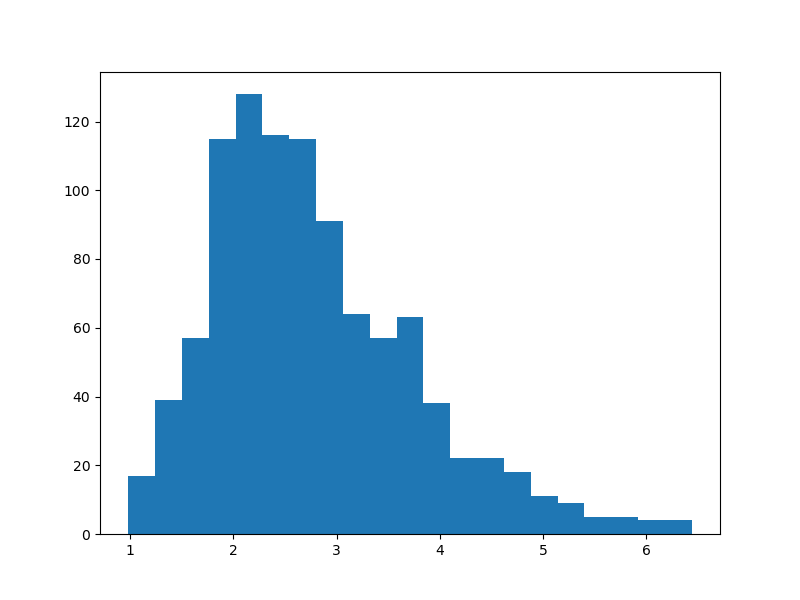
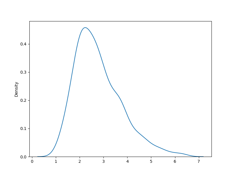
Figure 1: Asymptotic distribution for $d=1$

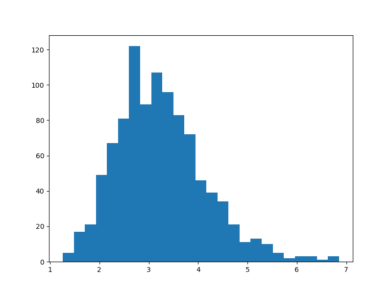
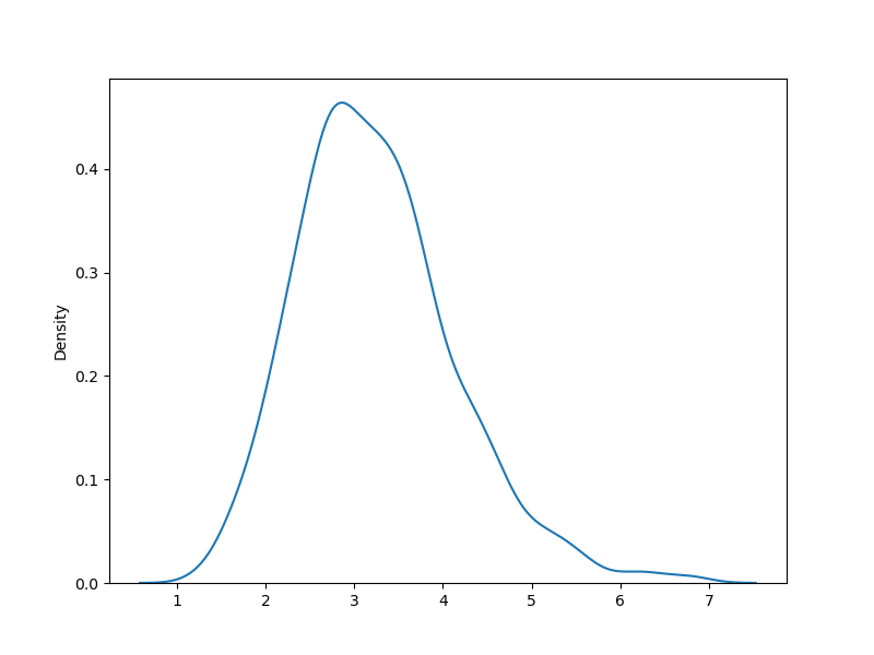
Figure 2: Asymptotic distribution for $d=2$

Given different significance levels, we obtain the asymptotic critical values of test statistics:

Sig. Level	Dimension 1	Dimension 2
0.99	1.84	1.604
0.95	1.485	1.964
0.90	1.717	2.199
0.10	4.102	4.419
0.05	4.705	4.840
0.01	5.740	5.835

Table 1: Critical Values for Different Significance Levels

5.1.2 Simulation evidence

Given two observed sequences of random variables $X,Y$, let $H_{0}$ be the hypothesis that $(X,Y)$ forms a martingale coupling, i.e. $\mathbb{E}[Y|X]=X$. We draw $n=100$ samples from each of the distributions and conduct $N=100$ replications to obtain the asymptotic size of the test. To see if our test is consistent, we consider the following test cases with $\alpha=0.05$. Recall that the Hermite polynomial of order $k$ is defined as $H_{k}(x)=(-1)^{k}e^{x^{2}/2}\mathrm{d}^{k}/\mathrm{d}x^{k}(e^{-x^{2}/2})$.

• Random Walk (NULL1): $X\sim\mathcal{N}(0,1)$, $Z\sim\mathcal{N}(0,1),Y=X+Z$.

• Hermite Polynomials (ALT1): $X\sim\mathcal{N}(0,1)$, $Y=X+H_{k}(X)/\sqrt{k!}$, where $k=1$.

• Hermite Polynomials (NULL2): $X\sim\mathcal{N}(0,1)$, $Y=X+H_{k}(X)/\sqrt{k!}$, where $k=20$.

Note that if $Z$ is standard Gaussian then $\mathbb{E}[H_{k}(Z)H_{\ell}(Z)]=0$ when $k\neq\ell$. If we let $(X,Y)=(Z,Z+H_{k}(Z))$, then $\mathbb{E}[(Y-X)X^{j}]=0$ for all $j=0,\dots,k-1$, and $\mathbb{E}[(Y-X)X^{k}]\neq 0$. The normalized version is $\mathbb{E}[Y^{2}]=\mathbb{E}[(Z+H_{k}(Z))^{2}]=1+\mathbb{E}[H_{k}(Z)^{2}]\asymp k!$, so we take $Y=Z+H_{k}(Z)/\sqrt{k!}$ instead. The results are summarized in Table 1, where $p$ denotes the empirical rejection rate and $\bar{T}$ represents the mean of the test statistic.

	$\alpha$	$N$	$n$	$p$	$\bar{T}$
NULL1	$0.05$	$100$	$100$	$0.00$	$1.643$
ALT1	$0.05$	$100$	$100$	$1.00$	$7.318$
NULL2	$0.05$	$100$	$100$	$0.01$	$1.804$

Table 2: Simulation Results with $\rho=5,\sigma=1$

5.1.3 The impact of $\sigma$

The parameter $\sigma$ plays an important role in our test. Varying values of $\sigma$ can have the following effects:

1. martingales are smoothed to different degrees;

2. martingale projection error is reduced at different rates;

3. the associated critical values change.

To see the smoothing effect of $\sigma$, consider a simple example of a martingale coupling $(B_{1},B_{2})$ where $\{B_{t}\}_{t\geqslant 0}$ is a Brownian motion. Figure 3 illustrates the impact of $\sigma=0.01$, $\sigma=0.1$, and $\sigma=1$ in smoothing martingale with $100$ samples.

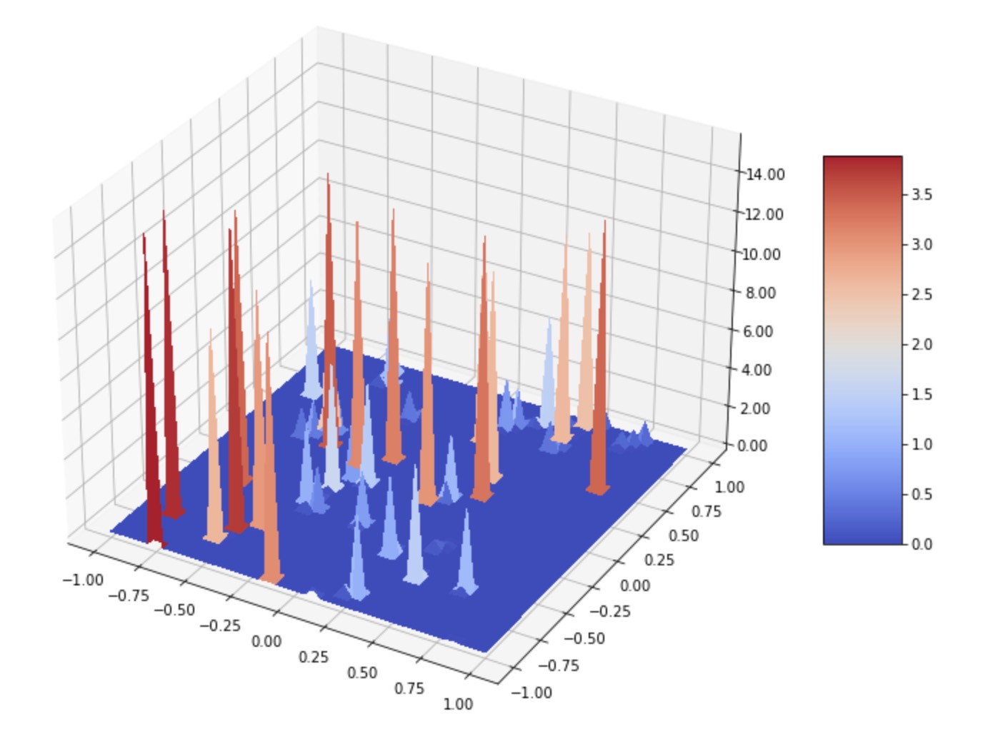
(a) $\sigma=0.01$

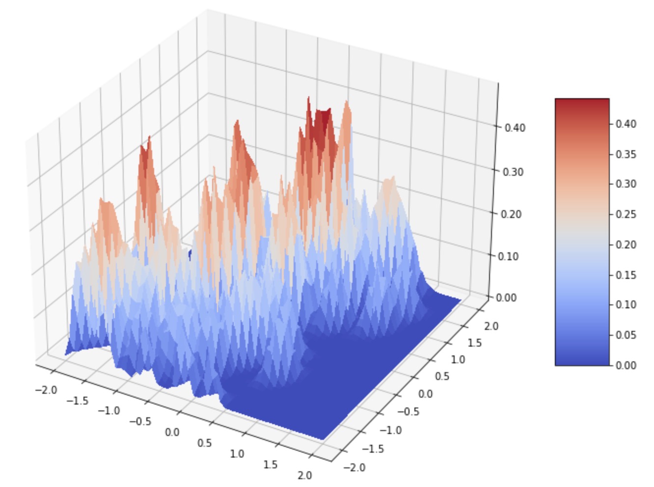
(b) $\sigma=0.1$

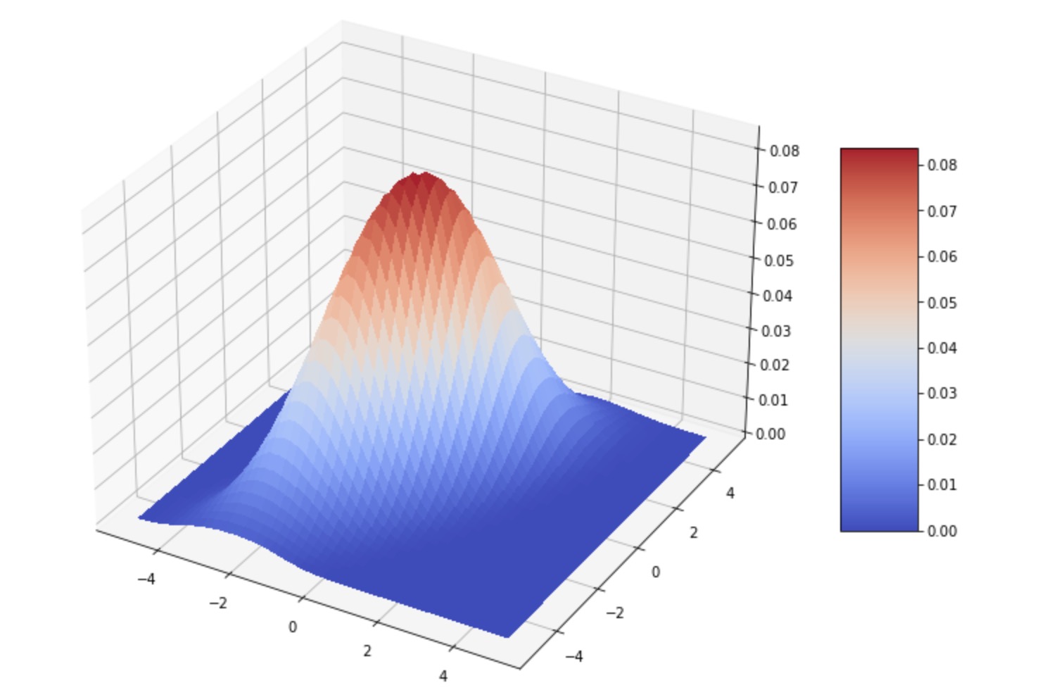
(c) $\sigma=1$

Figure 3: Effects of various $\sigma$ in smoothing a martingale coupling

In regards to (2), in general, the larger the value of $\sigma$, the faster the rate at which the martingale projection error is reduced, as shown in Figure 4 below. Here, we consider the same simple example of martingale coupling $(B_{1},B_{2})$ as in (1), and each graph plots 100 times the number of Monte-Carlo simulations we conduct ($x$-axis) against the resulting martingale projection error ($y$-axis) given different values of $\sigma$.

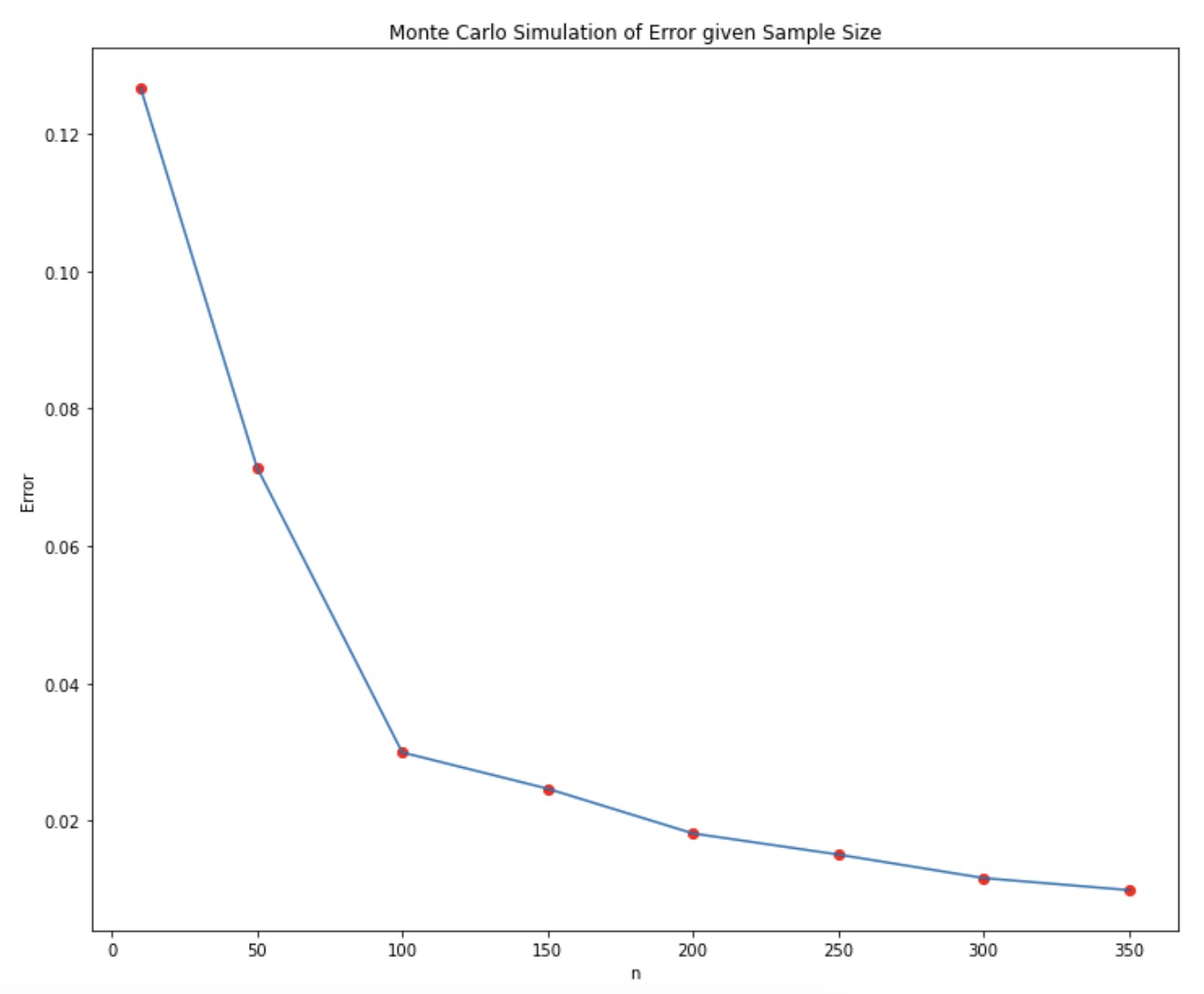
(a) $\sigma=0.1$

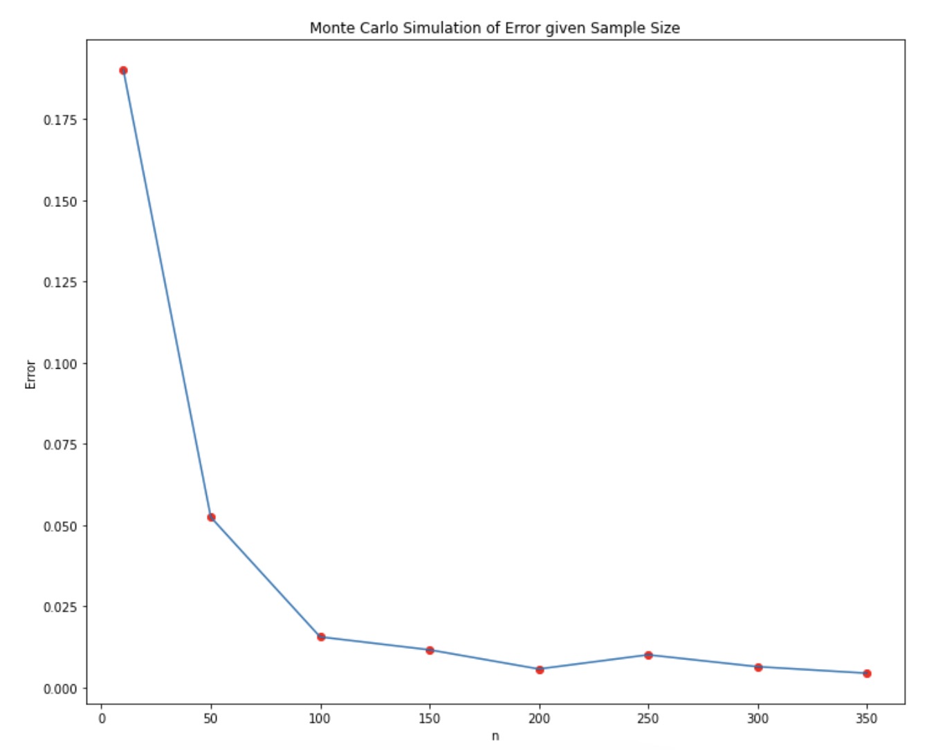
(b) $\sigma=1$

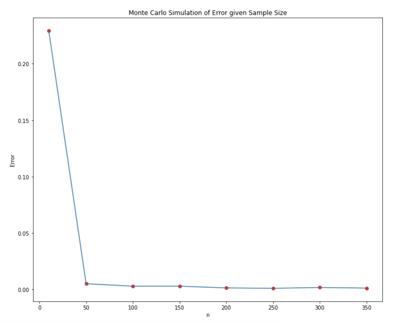
(c) $\sigma=2$

Figure 4: Effects of $\sigma$ in reducing projection error

For (3), as stated in Theorem 3, given a fixed significance level $\alpha$, the mean of the Gaussian random field integral decreases to $\asymp 1$ if $\sigma$ increases. Hence, the critical value is reduced. The augmented table below gives the simulated asymptotic critical values for $d=1$ and $1000$ replications with $\rho=5$ and $\sigma=0.01,1,100$ with Hermite couplings of varying degree $k$.

$\alpha$	$\sigma$	$c_{\alpha}$	$k$	$N$	$n$	$p$	$\bar{T}$
$0.05$	$0.01$	$15.006$	$1$	$100$	$100$	$0.00$	$10.000$
$0.05$	$1.00$	$4.705$	$1$	$100$	$100$	$1.00$	$7.318$
$0.05$	$100.00$	$1.980$	$1$	$100$	$100$	$1.00$	$10.000$
$0.05$	$0.01$	$15.006$	$5$	$100$	$100$	$0.00$	$3.781$
$0.05$	$1.00$	$4.705$	$5$	$100$	$100$	$0.10$	$3.910$
$0.05$	$100.00$	$1.980$	$5$	$100$	$100$	$1.00$	$3.982$
$0.05$	$0.01$	$15.006$	$10$	$100$	$100$	$0.00$	$2.778$
$0.05$	$1.00$	$4.705$	$10$	$100$	$100$	$0.00$	$2.733$
$0.05$	$100.00$	$1.980$	$10$	$100$	$100$	$0.98$	$2.639$
$0.05$	$0.01$	$15.006$	$15$	$100$	$100$	$0.00$	$2.106$
$0.05$	$1.00$	$4.705$	$15$	$100$	$100$	$0.00$	$2.183$
$0.05$	$100.00$	$1.980$	$15$	$100$	$100$	$0.45$	$2.078$
$0.05$	$0.01$	$15.006$	$20$	$100$	$100$	$0.00$	$1.813$
$0.05$	$1.00$	$4.705$	$20$	$100$	$100$	$0.01$	$1.804$
$0.05$	$100.00$	$1.980$	$20$	$100$	$100$	$0.08$	$1.747$

Table 3: Simulation results for Hermite couplings with $\rho=5$ and various $\sigma$

Immediately, we see that the choice of $\sigma$ has a significant influence on the power of the test. In general, the smaller the $\sigma$, the more lenient the test is (that is, the more likely the test is to commit Type I error). On the contrary, the larger the $\sigma$, the stricter the test is, so the more likely the test is to commit Type II error. This trade-off is illustrated by Figure 5, which plots the empirical rejection rate computed for a total of $10,000$ trials against different values of sigma on non-martingale example ALT1 with $k=5$.

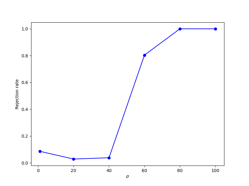
(a) rejection rate vs $\sigma$

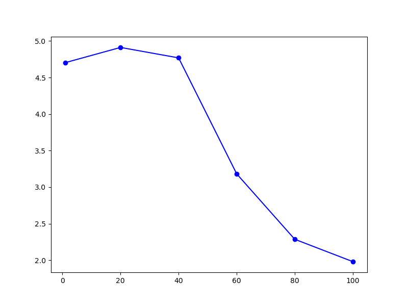
(b) critical value vs $\sigma$

Figure 5: Effects of $\sigma$ on the power of test

While the power of the test decreases slightly from $\sigma=1$ to $\sigma=20$, it increases consistently as $\sigma$ increases from $20$, with the biggest improvement taking place at $\sigma=60$.

5.1.4 Power curves for $d=1$

In this section, we plot the power curve with respect to a series of perturbed martingale couplings. We use $\rho=5$, $\sigma=80$ to conduct the tests.

• Model 1: Let $X\sim\mathcal{N}(0,1)$, $Z\sim\mathcal{N}(0,1)$, $Y=X+Z+\varepsilon$, where $\varepsilon\in\{-1,-0.75,-0.5,-0.25,0,0.25,0.5,0.75,1\}$.

• Model 2: $X\sim\mathcal{N}(0,1)$, $Y=X+H_{k}(X)/\sqrt{k!}$, where $k=1,4,7,10,13,16,19,22,25$.

Taking 1000 observations and using a replication size of 1000, we obtain the power curves for Model 1 in Figure 6 and Model 2 in Figure 7.

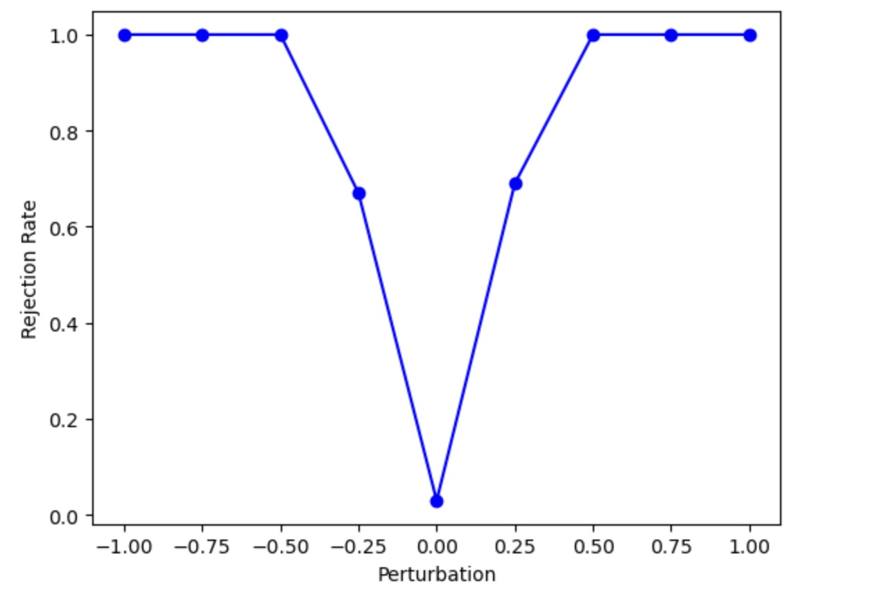
(a) Rejection rate vs perturbation

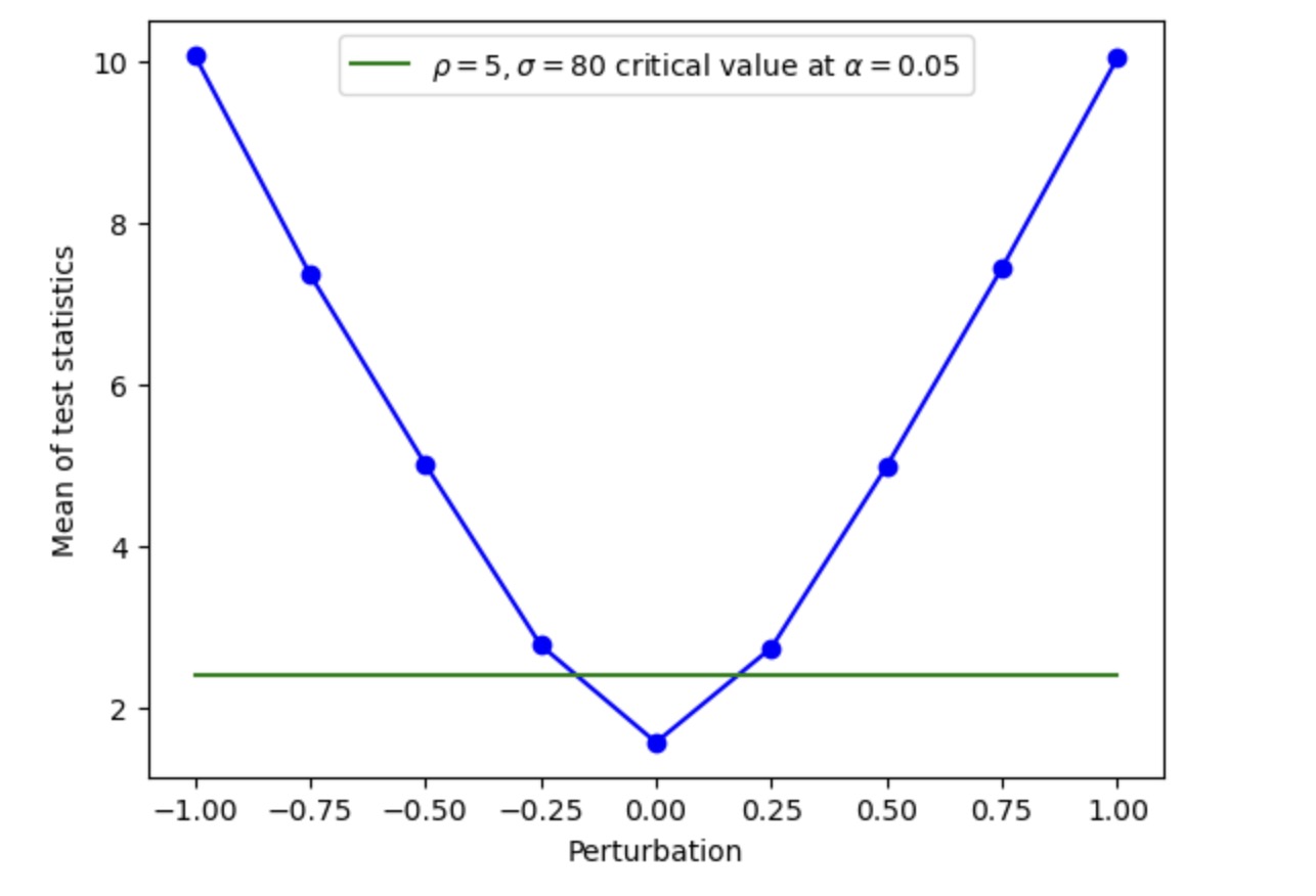
(b) Mean test statistics vs perturbation

Figure 6: Model 1

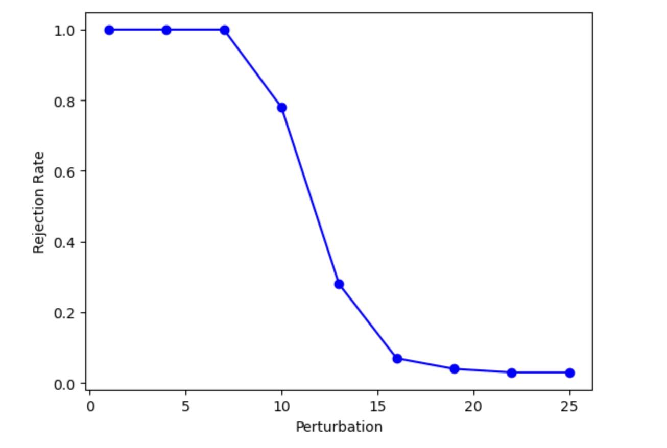
(a) Rejection rate vs $k$

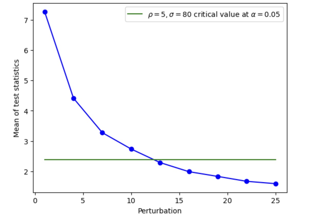
(b) Mean test statistics vs $k$

Figure 7: Model 2

5.2 Applications

Our hypothesis test for martingality provides valuable information in a wide range of areas of interest. For instance, it is well-known that martingales form an important pillar in financial economics and econometrics. For example, no-arbitrage conditions are equivalent in great generality to requiring the existence of a suitable probability measure under which discounted price processes follow martingale dynamics. Our results, therefore, can be used (as we shall illustrate) to test the no-arbitrage hypothesis in generative AI models.

A classical problem in econometrics and statistics consists of testing if a real-valued data set follows a given continuous distribution. The Kolmogorov-Smirnov statistic is a non-parametric approach to testing this hypothesis. A natural generalization of this problem consists of testing if a positive recurrent and irreducible general state-space Markov chain with stationary distribution $\phi$, $\left\{W_{n}:n\geqslant 0\right\}$, follows the transition kernel $\left\{K\left(x,\cdot\right):x\in S\right\}$. This is true if and only if for all continuous and bounded functions $u\left(\cdot\right)$ we have $\left(X_{n},Y_{n}\right)=\left(W_{n},W_{n}+u\left(W_{n+1}\right)-\left(Ku\right)\left(W_{n}\right)\right)$ forms a martingale pair for almost every $W_{n}$ with respect to $\phi$. Therefore, this hypothesis can be tested by selecting a family of functions $u_{1},\dots,u_{d}$ and testing the martingale property for the pair of $d$-dimensional vectors $\left(X_{n},Y_{n}\right)\in\mathbb{R}^{d}\times\mathbb{R}^{d}$, where $X_{n}\left(i\right)=W_{n}$ and $Y_{n}\left(i\right)=W_{n}+u_{i}\left(W_{n+1}\right)-\left(Ku_{i}\right)\left(W_{n}\right)$.

The above two applications of our test will be respectively detailed in this section below and Appendix A. There are numerous other applications of martingale pair tests in the sphere of finance, econometrics, reinforcement learning, and non-parametric regression. We briefly discuss a few instances below.

In the context of model-based reinforcement learning, a simulation environment generated according to a suitable family of Markov kernels $K_{\theta}$ (indexed by a parametric family of policies encoded by the parameter $\theta$) can be used to train an optimal control policy for the task at hand and an associated optimal value function $v$, which solves a corresponding HJB equation. A suitable transformation of the value function $v$ (similar to that discussed in the previous paragraph for $u$) can be obtained based on its associated HJB equation to define a pair $(X_{n},Y_{n})$ following a martingale sequence in the optimized simulation environment. If the simulated environment closely reflects the true environment, our results can be used to test if such a policy generates the desired performance (i.e. the predicted value $v$) in a real environment by applying the policy and also transformation in the real environment, collecting the generated data in an experiment in the true environment, and testing the martingale hypothesis in the data collected by the use of the policy in the true environment.

Other applications include assessing the quality of a non-parametric regression function. Suppose that a non-parametric estimator of $g(Z)=\mathbb{E}[Y|Z]$ based on observations ${(Z_{i},Y_{i}):i\leqslant n}$ is produced. Now consider the problem of evaluating the quality of such a non-parametric estimator, say $f_{0}$. We may consider defining $X=f_{0}(Z)$ and then testing whether the corresponding empirical measure $\mathbb{P}_{n}$ of pairs $(X_{i},Y_{i})=(f_{0}(Z_{i}),Y_{i})$ is sufficiently close to the martingale space. Moreover, as we shall explain, the power analysis of the martingale projection test also provides insight into how the martingale property fails to be satisfied. This may suggest a way to improve regression estimation training.

5.2.1 Testing no-arbitrage in neural SDE-based European option calibration

One application of our results is a test for arbitrage opportunities in existing pricing models for financial derivatives. In the following, we first describe the set-up of the financial market considered and then outline our methodology.

The work of [gierjatowicz2020robust] develops a neural SDE-based European option calibration method. In their set-up, the true dynamics of $X$ under the risk-neutral measure $\mathbb{Q}=\mathbb{Q}(\theta)$ are given by

$$\mathrm{d}X^{\theta}_{t}=b(t,X^{\theta}_{t},\theta)\mathrm{d}t+\sigma(t,X^{\theta}_{t},\theta)\mathrm{d}W_{t}$$ (59)

for functions $b:\mathbb{R}_{+}\times\mathbb{R}^{d}\times\Theta\rightarrow\mathbb{R}^{d}$ and $\sigma:\mathbb{R}_{+}\times\mathbb{R}^{d}\times\Theta\rightarrow\mathbb{R}^{d\times n}$, where $\Theta\subseteq\mathbb{R}^{p}$ for some $p>0$.

In order to calibrate asset prices consistently with the real-world measure $\mathbb{P}(\theta)$, [gierjatowicz2020robust] introduces a feed-forward neural network trained on market data, given by $\zeta:[0,T]\times\mathbb{R}^{d}\times\mathbb{R}^{p}\rightarrow\mathbb{R}^{n}$. Let $d_{K}$ represent the discounted payoff of a call option with strike $K$. The authors assume that the call prices at time zero

$$\mathfrak{p}(d_{K}):=\mathbb{E}^{\mathbb{Q}(\theta)}[d_{K}]=e^{-rT}\mathbb{E}^{\mathbb{Q}(\theta)}\left[\left(S_{T}-K\right)_{+}\mid S_{0}=1\right]$$ (60)

are given, and they calibrate (59) to $\mathfrak{p}(d_{K})$ through finding $\theta^{*}$ such that

$$e^{-rT}\mathbb{E}^{\mathbb{Q}(\theta^{*})}\left[\left(S_{T}-K\right)_{+}\mid S_{0}=1\right]\approx\mathfrak{p}(d_{K}).$$

Importantly, [gierjatowicz2020robust] only calibrates to call prices at time zero and does not take any other market data into account. In practice however, it is reasonable to assume that, next to the price process $(S_{t})_{t\in\{0,...,T\}}$, one should also be able to observe the corresponding option prices

$$\mathfrak{p}(d_{K},S_{t})=e^{-rT}\mathbb{E}^{\mathbb{Q}(\theta)}\left[\left(S_{T}-K\right)_{+}\mid S_{t}\right]$$ (61)

for $t\in\{0,\dots,T\}$ instead. Armed with our martingale pair test, we will check if the calibration procedure of [gierjatowicz2020robust] is consistent with the additional prices given in (61). In other words, does

$$\mathfrak{p}(d_{K},S_{t})\approx e^{-rT}\mathbb{E}^{\mathbb{Q}(\theta^{*})}\left[\left(S_{T}-K\right)_{+}\mid S_{t}\right]?$$

Our objective is to test if $(\mathfrak{p}(d_{K},S_{t}),e^{-rT}\left(S_{T}-K\right)_{+})$ is a martingale coupling under $\mathbb{Q}(\theta^{*})$ (which is necessary for (61)) for vanilla options. Our task is composed of three steps:

1. Calibrate asset prices for each time-step following the algorithms of [gierjatowicz2020robust]. Obtain $N$ calibrated stock trajectories $\{S_{t}\}_{t\in[0,\dots,T]}.$

2. Given a stock trajectory $\{S_{t}\}_{t\in[0,\dots,T]}$ from step one, use Monte Carlo simulation to obtain prices of vanilla options $\mathfrak{p}(d_{K},S_{t})$ at each $t\geqslant 0$ using (61).

3. Apply the martingale pair test to check if $(\mathfrak{p}(d_{K},S_{t}),e^{-rT}\left(S_{T}-K\right)_{+})$ is a martingale coupling under $\mathbb{Q}(\theta^{*}).$

The work of [gierjatowicz2020robust] used two market models for calibration: the local stochastic volatility model (LSV) and the local volatility model (LV). For step one, we alter the training algorithm of [gierjatowicz2020robust] for both LSV and LV models to return $N=4000$ calibrated stock trajectories $\{(S_{t})_{t\in[0,\dots,T]}^{i}\}_{i=1}^{N}$ directly. The altered codes, along with the implementation codes can be found on GitHub. For step two, for each stock trajectory $\{S_{t}\}_{t\in\{0,...,T\}}$, we use Monte Carlo simulation to generate $n=1000$ asset price paths using the true Heston model approximated via a tamed Euler scheme at each time point $t\in\{0,...,T\}$:

$$\mathrm{d}S_{t} =rS_{t}\mathrm{d}t+S_{t}\sqrt{V_{t}}\mathrm{d}W_{t},\ \ X_{0}=x_{0}$$

$$\mathrm{d}V_{t} =\kappa(\mu-V_{t})\mathrm{d}t+\eta\sqrt{V_{t}}\mathrm{d}B_{t},\ \ V_{0}=v_{0}$$

$$\mathrm{d}\langle B,W\rangle_{t} =\rho\mathrm{d}t.$$

We use the same set of parameters as [gierjatowicz2020robust]: $\theta=\{x_{0}=1,r=0.025,V_{0}=0.04,\kappa=0.78,\mu=0.11,\eta=0.68,\rho=0.044\}$. We then calculate the associated discounted European option prices with each maturity $T$ and strike $K$ by

$$\mathfrak{p}(d_{K},S_{t}):=e^{-rT}\mathbb{E}^{\mathbb{Q}(\theta)}[(S_{T}-K)^{+}|S_{t}]$$

In addition, we also calculate the calibrated payoff using [gierjatowicz2020robust]’s formula in (60). The algorithm is in Appendix B.

For the final step, we conduct a martingale pair test of the coupling $(\mathfrak{p}(d_{K},S_{t}),e^{-rT}\left(S_{T}-K\right)_{+})$ fixing $\sigma=1,\rho=5$ and a significance level of $\alpha=0.05$. We adapt the testing procedures outlined in Algorithm LABEL:algo:mtgl_pair_test. Codes for the martingale pair test can be found on our GitHub.

We find that, both for LV-model-based calibration and LSV-model-based calibration, $(\mathfrak{p}(d_{K},S_{t}),e^{-rT}\left(S_{T}-K\right)_{+})$ do not form martingales. For the LV model and the LSV model, the test statistics are 17.242 and 11.714 respectively, against an $\alpha=0.05$ critical value $c_{\alpha}=$ 4.705. In conclusion, [gierjatowicz2020robust]’s calibration method is shown to be inconsistent with the market data available.

We also observe that one of the [gierjatowicz2020robust]’s key contributions using hedging strategy as a control variate for the calibration model fails to work when we examine option prices as a function of the stock price observed at each time point. Instead, to avoid creating arbitrage opportunities in option prices (61), we propose the following neural SDE-based option calibration method: as before, the market data (input data) is represented by (discounted) payoffs $\{d_{K_{i}}\}_{i=1}^{M}$ of liquid derivatives and their corresponding market prices $\{\mathfrak{p}(d_{K_{i}})\}_{i=1}^{M}$. We then replace the loss function [gierjatowicz2020robust, equation (2.5)] by a martingale projection loss criterion:

$$\theta^{*}\in\text{arg min}_{\theta\in\Theta}\sum_{j=1}^{M}\sum_{i=1}^{N}\int\Big{(}(\mathfrak{p}({d_{K}}_{j},S^{\theta}_{t_{i}})-{d_{K}}_{j}(S_{t_{i}+\tau}^{\theta}))f_{\xi}(x-{d_{K}}_{j}(S_{t_{i}+\tau}^{\theta}))\Big{)}^{2}\,\mathrm{d}x.$$

The tentative new algorithm described by the pseudo-code can be found in Appendix B.

Appendix A Testing concurrence of a Markov chain with given transition kernel

We consider the problem of testing if an ergodic sequence follows a particular Markov chain dynamics. This problem is the analogue to the problem of testing if an i.i.d. sequence follows a particular distribution. In the one-dimensional i.i.d. setting, the Kolmogorov-Smirnov test provides a well-known approach.

Precisely, we are interested in testing if a $\phi$-irreducible and positive recurrent Markov chain sequence $\left\{W_{n}:n\geqslant 0\right\}$ taking values on a state-space $S$ (e.g. the support of $\phi$, which may be assumed to be a maximal irreducible measure) follows a particular transition kernel, $\left\{K\left(x,\cdot\right):x\in S\right\}$. This is true if and only if for all continuous and bounded functions $u\left(\cdot\right)$ we have that

$$\left(X_{n},Y_{n}\right)=\left(W_{n},W_{n}+u\left(W_{n+1}\right)-\left(Ku\right)\left(W_{n}\right)\right)$$

forms a martingale pair for almost every $W_{n}$ with respect to $\phi$. Indeed, if the ergodic chain satisfies this condition we have that for all continuous and bounded functions $u\left(\cdot\right)$

$$\left(Ku\right)\left(W_{n}\right)=E\left[u\left(W_{n+1}\right)|W_{n}\right]$$

almost everywhere with respect to the stationary measure which is a maximal irreducible measure (see Theorems 10.0.1 and 10.1.2 in [meyn2009]).

As an application of our results in this paper, we can select a family of continuous and bounded functions $u_{1},\dots,u_{d}$ so we can test the martingale property for the pair of $d$-dimensional vectors $\left(X_{n},Y_{n}\right)\in\mathbb{R}^{d}\times\mathbb{R}^{d}$, where

$$X_{n}\left(i\right)=W_{n},\text{ }Y_{n}\left(i\right)=W_{n}+u_{i}\left(W_{n+1}\right)-\left(Ku_{i}\right)\left(W_{n}\right).$$

To put the discussion into context, we consider a simple Gaussian Markov process and an example inspired by the present value process of perpetual cash flow as described in Example 2.2 of [gjessing1997present].

Example 8 (Gaussian Markov Process).

Consider the simple case of an infinite state space Gaussian Markov Process as the following:

$$X_{n+1}=\kappa X_{n}+\xi_{n+1},$$

where $\kappa\in[0,1]$, $\xi_{n+1}\sim\mathcal{N}(0,1)$ for each $n\in\mathbb{N}$.

Choosing $u_{1}(x)=x$ and $u_{2}(x)=x\mathds{1}_{\{x>0\}}$, we generate $\{(X_{n},X_{n+1})\}_{n=1}^{1000}$ with $\kappa=0.5$. For a martingale pair test with parameters $\{\rho=5,\sigma=1,\alpha=0.05\}$, the loss of the series of couplings is 3.091e-23 against an asymptotic cutoff value of 4.840. Hence, the test correctly accepts the series $\{(X_{n},X_{n+1})\}_{n=1}^{1000}$ as a martingale with 95% confidence.

Example 9 (Adapted present value process of perpetual cash flow).

Consider the stochastic process

$${Z}_{t}\ =e^{-rt}\Big{(}Z_{0}+\int_{s=0}^{t}e^{rs}\mathrm{d}{P_{s}}\Big{)}$$ (62)

where $t\geqslant 0$, $r>0$, $Z_{0}=0$, and ${P}_{t}=\sum_{i=1}^{N_{P,t}}S_{P,i}$ is a non-negative compound Poisson process with $N_{P,t}\sim\text{Pois}(\lambda_{P})$ and $S_{P,i}\sim\Gamma(\alpha,\beta)$. Choose $r=1$, $\lambda_{P}=2$ and $(\alpha,\beta)=(2,3)$, where $\alpha$ denotes the location parameter and $\beta$ denotes the scale parameter.

To generate the Markov chain, we use the observation that

$$Z_{t+1}=Z_{t}+\int_{s=0}^{1}e^{r(s-t)}\mathrm{d}P_{t+s}.$$

Choosing $u_{1}(x)=x$ and $u_{2}(x)=x\mathds{1}_{\{x>0\}}$, we generate $\{(Z_{t},Z_{t+1})\}_{t=1}^{1000}$. For a martingale pair test with parameters $\{\rho=5,\sigma=1,\alpha=0.05\}$, the loss of the series of couplings is 1.036 against an asymptotic cutoff value of 4.840. Hence, the test correctly accepts the series $\{(Z_{t},Z_{t+1})\}_{t=1}^{1000}$ as a martingale with 95% confidence.

It is interesting to note that the modified version of stochastic process (62)

$$Z_{t}=\int_{0}^{t}e^{-rs}\mathrm{d}P_{s}$$

has financial implications. In this case, ${Z}_{\infty}$ has the following density (see [gjessing1997present]):

$$f_{{Z}_{\infty}}=\alpha^{\frac{1}{2}(1+\gamma)}\gamma^{\frac{1}{2}(1-\gamma)}e^{-\gamma}z^{\frac{1}{2}(\gamma-1)}I_{\gamma-1}(2\sqrt{\alpha\gamma z})e^{\alpha z},$$

where $\gamma={\lambda_{P}}/{r}$ and $\lambda_{P}$ denotes the intensity of $N_{P,t}$, and $I$ is the modified Bessel function of the first kind of order $\gamma$:

$$I_{\gamma}(x)=(\frac{x}{2})^{\gamma}\sum_{k=0}^{\infty}\frac{1}{k!\Gamma(k+\gamma+1)}(\frac{x}{2})^{2k}.$$

In an actuarial context, ${P}_{t}$ is interpreted as the surplus generating process and ${Z}_{\infty}$ represents the present value of perpetual cash flow with respect to ${P}_{t}$.

Appendix B Deferred algorithms

Algorithm 1 Simulate Asymptotic Distribution given $\{\rho,\sigma\}$

Input: total number of grid points $n$ per dimension $d$, total number of simulations $N$, domain of integration $[x_{\min},x_{\max}]^{d}$, samples of martingale couplings $(X,Y)$, martingale projection parameters $\{\rho,\sigma\}$.
Initialization: initialize grid $g=\{g_{1},\dots,g_{n^{d}}\}$ based on domain of integration $[x_{\min},x_{\max}]^{d}$ and number of grid points $n$, smoothing kernel $f_{\sigma,\xi,\rho}$ as defined in (4).

Given samples $(X,Y)$, grid $g$, and $f_{\sigma,\xi,\rho}$:

for index $i$ $1:n^{d}$ do

     for index $j$ $1:n^{d}$ do

         Generate each entry $(i,j)$ of the covariance matrix $M_{n\times n}$ of Gaussian random field $\{G_{x}\}$:

$$\mathbb{E}[G_{g_{i}}G^{T}_{g_{j}}]=\mathbb{E}[(Y-X)f_{\sigma,\xi,\rho}(g_{i}-X)f_{\sigma,\xi,\rho}(g_{j}-X)(Y-X)^{T}].$$

     end for

end for

for index $i$ $1:N$ do

     Compute a sample

$$S_{i}=\int_{x\in g}\|G_{x}\|_{2}\mathrm{d}x.$$

end for

return $\{S_{i}\}_{i=1}^{N}$.