Using spatial extreme-value theory with machine learning to model and understand spatially compounding extremes

Abstract

When extreme weather events affect large areas, their regional to sub-continental spatial scale is important for their impacts. We propose a novel methodology that combines spatial extreme-value theory with a machine learning (ML) algorithm to model weather extremes and quantify probabilities associated with the occurrence, intensity and spatial extent of these events. The model is here applied to Western European summertime heat extremes. Using new loss functions adapted to extreme values, we fit a theoretically-motivated spatial model to extreme positive temperature anomaly fields from 1959–2022, using the daily 500-hpa geopotential height fields across the Euro-Atlantic region and the local soil moisture as predictors. Our generative model reveals the importance of individual circulation features in determining different facets of heat extremes, thereby enriching our process understanding of them from a data-driven perspective. The occurrence, intensity, and spatial extent of heat extremes are sensitive to the relative position of individual ridges and troughs that are part of a large-scale wave pattern. Heat extremes in Europe are thus the result of a complex interplay between local and remote physical processes. Our approach is able to extrapolate beyond the range of the data to make risk-related probabilistic statements, and applies more generally to other weather extremes. It also offers an attractive alternative to physical model-based techniques, or to ML approaches that optimise scores focusing on predicting well the bulk instead of the tail of the data distribution.

This manuscript was compiled on

Extreme weather events have adverse impacts on society and nature, and their impacts can be amplified when the events are temporally or spatially compounding (1, 2, 3). Extreme heat events are examples of such high-impact weather events as they affect crops, severe wildfires, energy demand, transportation, human mortality and more (e.g., 4, 5, 6, 7). The record-breaking impacts of the European heatwaves of 2003, 2010, 2018 and 2022 resulted from events of outstanding intensity and large spatial extent (8, 9, 10, 11, 12, 13, 14, 15, 16).

Several methods relying on physics-based numerical models have been recently proposed to study very extreme and very rare weather events, namely to utilise reforecast archives (17) or ensemble reinitialising (18, 19). However, the computational costs still limit the number of weather events that can be simulated, which makes it challenging to assess the probabilities of events with very extreme intensity or spatial extent in the current climate, let alone in a changing one.

In parallel, rapid progress has been made in the quality of machine learning (ML)-based weather forecasts, such as with the introduction of FourCastNet (20), Pangu-Weather (21) and Graphcast (22). These models have much lower computational costs and can in principle simulate thousands of years of weather evolution in a short amount of time. However, these methods are trained to minimise the root mean squared error, which inherently assumes the target of interest is the conditional mean. This may not be suitable when the focus is on extreme values, and can lead to unsuitable penalisation of extreme forecasts and inaccurate predictions of their spatial extent (23).

Our methodology proposes an alternative to the aforementioned approaches by only using data from the distributional tail to fit ML models that optimise new loss functions motivated by extreme-value theory (EVT); this theory provides an elegant and mathematically justified framework to estimate the probabilities of rare events by extrapolating beyond the range of the data. Modelling spatially dependent weather extremes is particularly challenging, and the sub-field of spatial EVT (24, 25) seeks to address this difficulty.

ML approaches offer attractive tools that use relevant predictors to provide computationally inexpensive and accurate predictions. We choose predictors based on physical and dynamical reasoning. For example, multiple physical processes are involved in the formation of heat extremes in the midlatitudes (e.g., 26, 27). On synoptic timescales, persistent large-scale anticyclones embedded in the midlatitude jet stream known as atmospheric blocks affect surface temperatures through horizontal temperature advection at their flanks, while adiabatic warming due to atmospheric subsidence and clear-sky radiative forcing can lead to enhanced warming and absence of precipitation in their center (28, 29, 30, 31, 32). Beneath the anticyclones, land–atmosphere feedbacks can further enhance temperatures, with low soil moisture limiting evaporative cooling (e.g., 33, 34, 35, 36, 37, 38). Figure 1 illustrates the atmospheric conditions during the European summer heatwave in July 2022, when temperatures rose above 40^∘C (more than 4 standard deviations away from the 1991–2020 climate) in UK for the first time. The large-scale circulation was characterized by a strongly meandering upper-level wave pattern, featuring a trough (negative Z500 anomaly) over the eastern Atlantic Ocean and an intense anticyclone (positive Z500 anomaly) over Europa. Underneath the anticyclone, a negative soil moisture anomaly was co-located with the heat extreme.

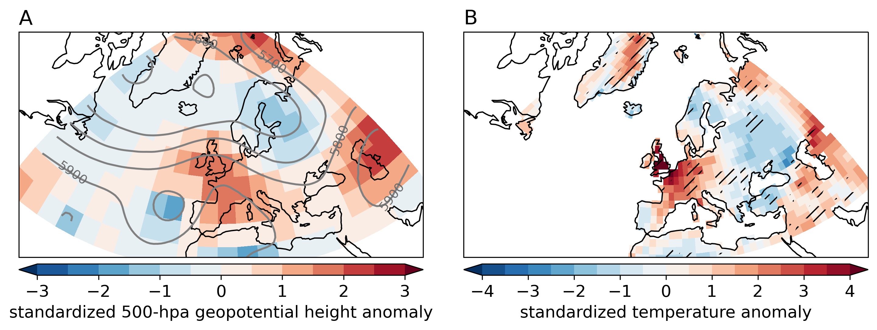
Figure 1: Characteristics of the 2022 European heatwave on July 19 from the ECMWF ERA5 reanalysis. (A) Standardized anomalies of 500-hPa geopotential height (shading interval -3 and 3) and absolute 500-hPa geopotential height contours (gray contour interval 5400m and 5800m every 100m), (B) Standardized anomalies of surface 2m temperature (shading interval -4 and 4) and standardized anomalies of soil moisture (hatching for area with $<-1$ STD).

The relevance of the above-mentioned processes varies across heat extremes (26), and they may interact in complex ways (39, 40, 41). The lack of physical understanding of these complex interactions during extreme-causing weather patterns impedes accurate prediction of heat extreme intensity and spatial extent (42, 32, 27). Our methodology seeks to address this knowledge gap.

ML tools have recently been combined with univariate EVT to predict conditional distributions above a high threshold, using gradient boosting (43, 44), random forest (45), and neural network architectures (46, 47). These studies rely on models like the Generalized Pareto distribution (GPD), but impose stringent spatial independence assumptions as they do not use theoretically motivated spatial models from spatial EVT. Furthermore, no studies have yet utilised more than two predictors to model the variation in the spatial dependence of extreme events using EVT.

Analogous to the role of the GPD in univariate EVT, generalised $r$-Pareto processes (48) are suitable models for spatial extremes, because they provide asymptotic approximations to the distribution of functional exceedances of appropriately re-scaled random fields; we provide more details on this in the next sections. Parametric forms of these processes have been developed, most notably the Brown–Resnick (49) model, which is based on Gaussian processes, and they have been shown to be flexible enough to capture complex spatial dependencies.

We develop novel ML models that predict the occurrence probability, the local intensity at each grid point (henceforth, just intensity), and the spatial extent of high-exceedance (extreme) temperature events, by fitting a Brown–Resnick $r$-Pareto process to our data. The proposed models quantify temporal non-stationarity in the spatial extremal dependencies, while also being the first attempt in literature to do so with the incorporation of many predictors - in our case, daily fields of atmospheric circulation patterns over the Euro-Atlantic region and local or regional soil moisture summaries. The predictors are included without needing to a priori select a set of reference patterns, e.g., EOF-derived weather regimes (e.g., 50). Inspection of variable importance in our fitted models thus enriches our process understanding of summertime heat extremes from a data-driven perspective.

Our methodology is generalisable to other ML approaches; we choose gradient boosting of regression trees (51) due to its automatic predictor selection feature and the ease at which non-linearities and predictor interactions are incorporated. It can also be used for other applications with appropriate care; here we showcase our methodology with a case study of heat extremes over western Europe.

Data

We use daily gridded data from the ECMWF ERA5 reanalysis (52) in the Atlantic–European region (60^∘W - 60^∘E, 30^∘N - 90^∘N) for the months of July to August (summer) over the period 1959–2022. From this data set, we use daily means of 2 m land surface air temperature (T2M), 500 hpa geopotential height (Z500) and soil moisture integrated over a depth of 28 cm (SM) at a horizontal longitude-latitude resolution of 1.875 degree (T2M and SM) and 5.625 degree (Z500). The ERA5 data can be downloaded freely from the Copernicus Climate Data Store at https://climate.copernicus.eu/climate–reanalysis.

The following preprocessing steps are applied to the daily standardized temperature anomalies (T2M) and predictors (Z500 and SM): The fields are first detrended by removing the linear trend for each grid point over the analysed baseline period (1959–2022). We then compute standardized anomalies by removing the climatological mean and dividing by its standard deviation (Figure 2A,B). The climatological mean and standard deviation are defined as the 31-day dunning mean and standard deviation, respectively, centered around each date of the year and averaged over the World Meteorological Organization-defined reference period 1991–2020.

The predictor Z500 is further temporally averaged over the previous 5-day period to remove higher frequency components, i.e., transient Rossby waves, and to isolate persistent larger-scale circulation patterns. Similarly, the predictor SM is temporally averaged over the previous 15-day period.

Our modelling procedure is based on first identifying which events are extreme, which we do so based on the spatial average of daily standardized temperature anomalies over all grid points in a target region (see the region indicated in Figure 2). We select this region because it encompasses areas with high population density and includes major cities such as London, Amsterdam, and Paris. We say that an event is extreme if this spatial average exceeds its $95^{\text{th}}$ percentile, giving us 272 events. We call such an event an $r$-exceedance, in line with the more general framework that we will describe later. Percentile-based definitions of heat extremes are widely used (53, 54), but our approach differs from univariate definitions of extremes such as grid point-wise exceedances which renders the analysis of spatial extremal dependence difficult.

Let $y^{\prime}_{t}\in\{0,1\}$ denote the indicator equal to one if there is an $r$-exceedance on day $t$, and zero otherwise, and let $\mathcal{T}$ be the set of days where $y^{\prime}_{t}=1$. The schematic overview of our full model is displayed in Figure 2, and is composed of three sub-models which we detail later. The first analyses the occurrence probability of an $r$-exceedance, which uses the binary data $y^{\prime}_{t}$, for all days $t$. The second and third sub-models focus specifically on the extreme events, and so only considers the field (in practice, finite-dimensional data vector) of the T2M response for all $t\in\mathcal{T}$. These two sub-models allow us to quantify different facets related to the $r$-exceedances’ local intensity, e.g., the exceedance probability of T2M being large at a grid point, or their spatial dependencies, e.g., the joint probability of T2M being simultaneously large at several grid points. We use the years 1959–2017 for training, while the years 2018–2022 are used for testing the model performance.

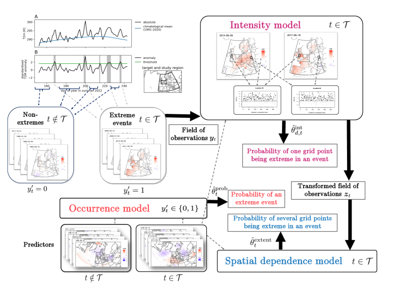
Figure 2: Schematic overview of our sub-models, to complement the description in the Data and Methods and models sections. Top left displays (A) temporal evolution of absolute value in summer 2022 (black) and climatological mean (blue, 1991–2020) for T2M (K) averaged over the target region. (B) Temporal evolution of standardized T2M anomaly (STD) in summer 2022 averaged over the target region (black, with respect to climatological mean) and 95th percentile threshold (green) used for the definition of hot extremes (gray shaded) in the target region. The target and study region are shown on the map in the middle. The occurrence sub-model (in red), takes as input the binary data $y^{\prime}_{t}$, for all time points t, and outputs the probability of an $r$-exceedance. The intensity sub-model (in purple), takes as input the the data vector of the T2M response $\bm{y}_{t}$, $t\in\mathcal{T}$, and outputs the probability of each grid point exceeding a high threshold at each grid point. The spatial dependence sub-model (in blue), takes as input the transformed field of observations $\bm{z}_{t}$, $t\in\mathcal{T}$, and outputs the probability of simultaneous exceedances at several grid points. For the full description of the sub-models, see the text.

Methods and models

Our proposed methodology uses $r$-Pareto processes, which facilitate the assessment of individual daily functional exceedances of entire spatial fields. We develop this framework to incorporate predictors in a ML algorithm at the same daily resolution as the response. Our spatial model differs from and is an extension of those in univariate EVT such as the GPD, which takes as response exceedances at each grid point; this neither considers their spatial dependencies nor the actual weather events, as the exceedances over a high local percentiles at each grid point do not necessarily happen on the same day.

While max-stable processes are now commonly used in spatial EVT, they are only suitable for modelling grid point-wise maxima fields, which can also overlook the co-occurrence of extreme events across multiple locations. Furthermore, only modelling maxima fields makes the goal of understanding the drivers of heat extremes at fine temporal resolution such as ours challenging.

Spatial exceedances

Let $S$ denote our study region, a compact subset of $\mathbb{R}^{2}$, $\mathcal{F}$ the space of real-valued continuous functions on $S$ and $\mathcal{F}_{+}$ the space of positive ones. Exceedances for the T2M random field $Y=\{Y(\bm{s}):\bm{s}\in S\}$ can be characterised using $r$-exceedances, and are defined as events $\{r(Y)\geq u\}$ for some threshold $u\geq 0$ and $r$ a continuous mapping from $\mathcal{F}$ into $\mathbb{R}$. As described in the previous section, we choose $r$ to be the spatial mean of the anomalies across our chosen target region $\mathcal{A}$, i.e., $r(Y)=\mid\mathcal{A}\mid^{-1}\int_{\mathcal{A}}Y(\mathbf{s})\text{d}(\mathbf{s})$. We assume that $X$ is generalised regularly varying, which, along with growth rate assumptions (detailed in 48), ensure that the tail limit processes for rescaled $Y$ converges to a generalised $r$-Pareto process (GrP), conditional on an increasingly large $r$-exceedances of $X$, i.e.,

$$\operatorname{Pr}\left[\frac{Y-b_{n}}{r\left(a_{n}\right)}\in\cdot\mid r\left({Y}\right)\geqslant u_{n}\right]\rightarrow\operatorname{Pr}(P\in\cdot),\quad n\rightarrow\infty,$$ (1)

where $\left\{a_{n}\right\}_{n=1}^{\infty}>0$ and $\left\{b_{n}\right\}_{n=1}^{\infty}$ are sequences of continuous functions, $u_{n}$ is an increasing sequence, and $P$ is a GrP with scale parameter $A>0$. In this work, we assume that $u_{n}$ being the $95^{\text{th}}$ percentile of the empirical realisations of $r(Y)$ is sufficiently high for (1) to hold, and this also lies within the range over which the estimated tail index for the realisations of $r(Y)$ is stable.

GrP based on Gaussianity

(1) shows that GrPs appear as theoretically motivated limiting models for $r$-exceedances, akin to the Generalized Pareto distribution (GPD) for univariate exceedances (55). These processes can be represented as (56):

$$P=\dfrac{\{RW/r(W)\}^{\xi}-1}{\xi},$$

where $\xi\in\mathbb{R}$ governs the marginal tail decay, and the scalar $R$ is unit Pareto and independent of the stochastic process $W$ which takes values in the unit $L_{1}$-sphere $\left\{y\in\mathcal{F}_{+}:\|y\|_{1}=1\right\}$.

A flexible class of models is the Brown-Resnick (49, 57), where $W$ is there a log-Gaussian process whose underlying Gaussian process is centered and intrinsically stationary. These models are attractive to furnish models for extremal dependence as they are completely characterised by the variogram of the Gaussian process $\gamma(\bm{s}_{1},\bm{s}_{2})=\operatorname{var}\left\{W\left(s_{1}\right)-W(s_{2})\right\}$, $\bm{s}_{1},\bm{s}_{2}\in S$, and in our study we use the anisotropic powered semivariogram

$$\tiny\gamma(\bm{s}_{1},\bm{s}_{2})=\left\{\dfrac{1}{\theta^{\text{extent}}}\left|\left|\begin{pmatrix}\cos\tau&-\exp(\theta^{\text{scale}})\sin\tau\\ \sin\tau&\exp(\theta^{\text{scale}})\cos\tau\end{pmatrix}(\bm{s}_{1}-\bm{s}_{2})\right|\right|\right\}^{\alpha},$$ (2)

where $\alpha\in(0,2]$, $\theta^{\text{extent}},\theta^{\text{scale}}\in\mathbb{R}$ and $\tau\in[0,2\pi]$. For a fixed $\alpha$, the parameters $\theta^{\text{extent}}$ and $\theta^{\text{scale}}$ can be interpreted in terms of the characteristic size of individual $r$-exceedance events; jointly, the two parameters also control the relative spatial extent in the east-west compared to the north-west direction. We here project the coordinates of the grid points to be on the kilometre scale.

This framework models the spatial extremal dependence of the entire temperature field. More succinctly, this dependence can be summarised in a pairwise fashion for grid points $\bm{s}_{1},\bm{s}_{2}\in\mathcal{S}$ as

$$\tiny\pi(\bm{s}_{1},\bm{s}_{2})=\operatorname{Pr}\left[Y\left(\bm{s}_{2}\right)>u_{q}\left(\bm{s}_{2}\right)\mid\left\{Y(\bm{s}_{1})>u_{q}(\bm{s}_{1})\right\}\cap\{r(Y)\geqslant u\}\right],$$ (3)

and is equal $2\left(1-\Phi\left[\{\gamma(\bm{s}_{1},\bm{s}_{2})/2\}^{1/2}\right]\right)$ when $q\rightarrow 1$ for the Brown-Resnick model, where $u_{q}(s)$ denotes the $q$ quantile of $Y(\bm{s})$, $u\geq 0$ is the chosen high threshold, and $\Phi$ denotes the standard normal cumulative distribution function. Given an $r$-exceedance and that the response at a grid point $\bm{s}_{1}$ exceeds a high threshold, (3) evaluates the probability that another grid point $\bm{s}_{2}$ also exceeds a high threshold.

The bottom panels of Figure 3 show two different simulations from a GrP on our spatial region with artificially low and high dependence, assuming the other parameters being equal.

Inference for GrP with predictors

Statistical inference for $r$-exceedances conditional on a random vector of predictors $\bm{X}$ is based on the approximation

$$\operatorname{Pr}(Y\in\mathcal{R}\mid\bm{X}) \approx{\operatorname{Pr}\left\{r(Y)\geq u\mid\bm{X}\right\}}\times{\operatorname{Pr}(P\in\mathcal{R}\mid\bm{X})},$$ (4)

where $\mathcal{R}\subset\mathcal{R}\left(u\right)=\left\{y\in\mathcal{F}:r(y)\geqslant u\right\}$.

Our full model is composed of three sub-models; one models the first term in (4), i.e., the probability of an $r$-exceedances, and two uses the T2M response from the days with an $r$-exceedance to model the last term involving the $r$-Pareto process $P$, i.e., the marginal intensity and spatial dependence in the $r$-exceedances of $Y$. Figure 2 displays the the schematic of all the sub-models.

Our sub-models for the last term of (4) builds a space-time model that consists, at each day, of an $r$-Pareto process whose marginal distributions and dependence structure can evolve with predictors. We assume conditional independence in our modelling procedure given the predictors, which still entails temporal dependence of the $r$-exceedances driven solely by the varying predictors. This assumption is realistic for our case study on heat, and it withholds the need to decluster our responses in time.

We use the whole Z500 field (all $242$ grid points) as predictors in all our sub-models. For the soil moisture predictor, we further spatially aggregated it over the target region for the occurrence sub-model. For the dependence sub-model, we spatially aggregated over four approximately equally-sized rectangles (see the four rectangles in Figure 7H) over the study region and consider each as a predictor. As the intensity is varying in both space and time, we use the latitude, longitude and soil moisture at each grid point as predictors for this sub-model.

Using these predictors, each sub-model is a ML model that we train with loss functions motivated by the aforementioned theory. We do this in the distributional boosting framework, which we describe next.

Distributional tree boosting

The development and dissemination of open-source packages such as gbm (58) and xgboost (59) have partly fueled the popularity of gradient tree boosting (51) methods over the last decade. When appropriately tuned and/or used in an ensemble with other ML approaches, these methods can give extremely accurate predictions in various classification and regression tasks (60).

Let $\{(\bm{x}_{t},\bm{y}_{t})\}$, $\bm{x}_{t}\in\mathbb{R}^{p}$, $\bm{y}_{t}\in\mathbb{R}^{D}$, $t=1,\dots,T$, be a dataset with $T$ pairs of a response with dimension $D\in\mathbb{N}$, and $p\in\mathbb{N}$ predictors. A gradient tree boosting model gives an estimate $\hat{\theta}$ that is a sum of regression trees (61), i.e.,

$$\hat{\theta}_{t}=\sum_{i=1}^{N}f_{i}(\bm{x}_{t}),\quad f_{i}\in\mathcal{T},$$ (5)

where $\mathcal{T}$ is the space of regression trees. In the parametric distributional boosting framework, $\hat{\theta}_{t}$ represents a vector of predicted parameters of a given model for the conditional distribution of the response given the predictors at time $t$. Other, assumption-free distributional boosting approaches have also been proposed (e.g., 62), though we do not tackle these here.

The set of trees used in (5) are usually learnt by minimizing a regularized objective function in a greedy iterative fashion; we add the tree that most minimizes an objective function $\mathcal{O}$ at each iteration. More precisely, let $\hat{\theta}_{i}^{(j)}$ be the boosting estimate for the $t$-th observation at the $j$-th iteration. Many variants of this algorithm exists, but a popular one by (63) uses a second-order approximation for the objective so a tree $f_{j}$ is added at each iteration to minimize

$$\sum_{t=1}^{T}{\left\{\mathcal{L}(\bm{y}_{t},\hat{\theta}_{t}^{(j-1)})+g_{t}f_{j}(\bm{x}_{t})+h_{t}f_{j}^{2}(\bm{x}_{t})\right\}}+\Omega(f_{j}),$$ (6)

where $\mathcal{L}$ is a differentiable loss function, $\Omega$ is a measure of complexity of the tree and it prevents overfitting, $g_{t}=\partial\mathcal{L}(y_{t},\hat{\theta}_{i}^{(j-1)})/\partial\hat{\theta}_{i}^{(j-1)}$ and $h_{t}=\partial^{2}\mathcal{L}(y_{t},z_{t})/\partial z_{t}^{2}\mid_{z_{t}=\hat{\theta}_{t}^{(j-1)}}$. Computational saving strategies dictate the forms of $\Omega$, and here we use that from (59).

We choose the number of trees $N$ for each of our boosting sub-models by random 5-fold cross-validation, and for parsimony, set the other hyperparameters of our boosting models at reasonable values (detailed in the SI).

Loss functions to model compound extremes

The loss $\mathcal{L}$ in (6) steers the models that we fit. For the losses we present here we also derive the closed analytical form of the gradient $g_{t}$ and hessian $h_{t}$ in (6), which facilitates quick computation; we compile them in the R package described in the SI.

Let $\bm{y}_{t}=(y_{1,t},\dots,y_{D,t})$ be realizations of the temperature anomaly field (T2M) $Y$ evaluated at grid points $s_{1},\dots,s_{D}\in\mathcal{S}$ and replicated over the days $t=1,\dots,T$. Recall that $y^{\prime}_{t}\in\{0,1\}$ is the indicator for an $r$-exceedance on day $t$, and that $\mathcal{T}$ contains all the days where $y^{\prime}_{t}=1$.

To model ${\operatorname{Pr}\left\{r(Y)\geq u\mid\bm{X}\right\}}$ in (1), we consider the response $y^{\prime}_{t}$ and predict the probability of occurence $\operatorname{logit}(\theta^{\text{prob}}_{t})\in[0,1]$ using the log-loss

$$\mathcal{L}_{\text{log-loss}}(y^{\prime}_{t},\hat{\theta}^{\text{prob}}_{t})= y^{\prime}_{t}\log\{\operatorname{logit}(\hat{\theta}^{\text{prob}}_{t})\}$$

$$+(1-y^{\prime}_{t})\log\{1-\operatorname{logit}(\hat{\theta}^{\text{prob}}_{t})\},$$

which is standard for modeling binary counts.

The other two sub-models predict ${\operatorname{Pr}(P\in\mathcal{R}\mid\bm{X})}$ in (4). Their fitting procedures proceed sequentially, as is common in copula modeling: we first estimate the marginal parameters and then fit the dependence model after standardizing the margins using their estimates from the previous step.

For the normalising functions in (1), we set the normalising threshold at each grid point to be temporally constant, i.e., $b_{n}(\bm{s}_{d};t)=b_{d}$, and write $A\times r\{a_{n}(\bm{s}_{d};t)\}=\exp(\theta_{d,t}^{\text{int}})$ for each $d\in\{1,\dots,D\}$. We follow (48) and choose $b_{d}$ to equal the empirical $q^{\prime}$ quantile at the location $\bm{s}_{d}$ of the $r$-exceedances, with $q^{\prime}$ chosen such that $r(b_{n})=u_{n}$. We obtain $q^{\prime}=0.27$, giving $20^{\prime}040$ individual excesses across all days and grid points.

The GPD loss likelihood has garnered recent interest from the EVT modelling community for training ML models (e.g., 44, 43, 45). We predict the scale parameter of the GPD ${\theta}_{l,t}^{\text{int}}\in\mathbb{R}$ governing the local excesses at each grid point by using a variant of this loss, i.e.,

$$\mathcal{L}_{\text{GPD}}(y_{d,t},\hat{\theta}_{d,t}^{\text{int}};\xi) =\mathbbm{1}_{t\in\mathcal{T}}\sum_{d=1}^{D}\mathbbm{1}_{y_{d,t}>b_{d}}\Bigg{[}\log\{\exp(\hat{\theta}_{d,t}^{\text{int}})-m_{d}\xi\}$$

$$+\dfrac{\xi+1}{\xi}\log\left\{1+\xi\dfrac{y_{d,t}-b_{d}}{\exp(\hat{\theta}_{d,t}^{\text{int}})-m_{d}\xi}\right\}\Bigg{]}.$$

The indicator $\mathbbm{1}_{t\in\mathcal{T}}$ above indicates that only the extreme days contribute to this loss. The parameter $m_{d}$ is an estimated upper bound that prevents violation of the support constraint of the GPD when $\xi<0$, which is common in environmental data. We set $m_{d}=\hat{\sigma}_{d}/\hat{\xi}_{d}$, where $\hat{\sigma}_{d}$ and $\hat{\xi}_{d}$, $d=1,\dots,D$, are the location-wise GPD maximum likelihood estimates of the positive exceedances from $y_{d,t}-\hat{b}_{d}$, $t\in\mathcal{T}$. We fixed the shape parameter $\xi$ to $-0.3$ due to our five-fold cross validation study (detailed in the SI); this is also close to the minimum score estimate unconditional on the predictors. A constant shape parameter over $\mathcal{S}$ is not unrealistic here as we are modelling only one type of tail regime of our temperature process governed by large-scale atmospheric circulation; model diagnostic plots of the fitted model on the test data (displayed later in Figure 6) confirms that this assumption is reasonable.

We concatenate our predictions and write $\hat{\bm{\theta}}_{t}^{\text{int}}=(\hat{\theta}_{1,t}^{\text{int}},\dots,\hat{\theta}_{D,t}^{\text{int}})$ and $\hat{\bm{b}}=(\hat{b}_{1},\dots,\hat{b}_{D})$. We transform our observations to $\bm{z}_{t}=\{1+(\bm{y}_{t}-\hat{\bm{b}})\xi/\exp(\hat{\bm{\theta}}_{t}^{\text{int}})\}_{+}^{1/\xi}=(z_{1,t},\dots,z_{D,t})$, $t=1,\dots,T$, and use these in the last sub-model to predict a measure of the spatial extent $\theta^{\text{extent}}_{t}\in\mathbb{R}$ from the variogram (2) of the Brown-Resnick model using the loss

$$\mathcal{L}_{\text{GrP}}(\bm{z}_{t},\hat{\theta}^{\text{extent}}_{t}) =\mathbbm{1}_{t\in\mathcal{T}}\sum_{d=1}^{D}\left\{w_{d}(z_{d,t})^{2}\dfrac{\partial\lambda_{\theta}(\bm{z}_{t})}{\partial z_{d,t}}\Bigl{|}_{\theta=\hat{\theta}^{\text{extent}}_{t}}\right\}+$$

$$2\dfrac{\partial}{\partial z_{d,t}}\left\{w_{d}(z_{d,t})^{2}\dfrac{\partial\lambda_{\theta}(\bm{z}_{t})}{\partial z_{d,t}}\Bigl{|}_{\theta=\hat{\theta}^{\text{extent}}_{t}}\right\},$$ (7)

where $w_{d}:\mathbb{R}_{+}\rightarrow\mathbb{R}_{+}$ is the positive weight function derived in (64), and $\lambda_{\theta}$ is the intensity function detailed in (65), which here depends on the variogram parameters in (2). (Loss functions to model compound extremes) is based on the gradient scoring rule (66) derived for the Brown-Resnick model in (48), but here adapted to incorporate temporal non-stationarity via predictors. The rotation parameter $\tau$ in (2) is fixed to zero for parsimony, while $\alpha$ and ${\theta}_{t}^{\text{scale}}$ chosen to be temporally constant at 1.27 and -0.07 respectively, which are their corresponding minimum gradient score estimates from the model fitted without the predictors. Instead of keeping it fixed, one could also predict $\theta_{t}^{\text{scale}}$ in the algorithm by replacing $\hat{\theta}_{t}^{\text{extent}}$ with $\hat{\theta}_{t}^{\text{scale}}$ in (Loss functions to model compound extremes), and apply our fitting procedure consecutively between the two parameters after each iteration. However, we choose a more parsimonious approach in our data scarce setting and only allow $\hat{\theta}_{t}^{\text{extent}}$ to vary with predictors.

The numerical complexity of (Loss functions to model compound extremes) is that of matrix inversion, i.e., $\mathcal{O}(D^{3})$. To facilitate quicker computation, we construct numerically convenient representations of Gaussian processes using the Vecchia approximation (67) with $k$ conditioning variables; this sparsifies the Cholesky factor of the precision matrix to reduce the computational cost to $\mathcal{O}(Dk^{3})$ when $k\ll D$. Here we use the ordering outlined in (68) which improves on the lexicographic one original proposed, and our numerical results suggest that taking $k\approx 20$ is reasonable. Detailed in the SI, we check by simulation that the parameters are identifiable and can be predicted adequately in a setting similar to ours. Such verification is especially important for the last sub-model due to to its complexity, and since detecting non-stationarity in the extremal spatial dependence structure is challenging with too few data.

Results

Model simulation and evaluation on the test set

A key feature of our ML model grounded in EVT is that it is generative. It allows us to simulate a range of extreme weather scenarios by varying predictor conditions and also to explore theoretically-driven alternative scenarios under fixed predictor conditions, thereby extending the model’s utility beyond mere prediction. We achieve this generative capability of the ML model using a modified version of the algorithm proposed in (48), here allowing for predictors.

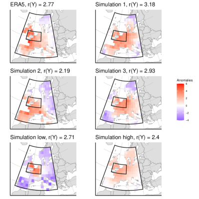
Figure 3: ERA5 realisation of the surface temperature anomaly (top left panel) and model simulations (top right and middle panels) on 18 July 2022 given an $r$-exceedance. The subtitle in each panel indicates the spatial average of T2m over all grid points in the target region. The bottom panels show simulations from a GrP with all the same model-predicted parameters except for $\theta_{t}^{\text{extent}}$, which we artificially set to a low of 0.05 and a high of 4; our model instead predicted $\hat{\theta}_{t}^{\text{extent}}=1.81$. A grey fill at a grid point in the study region indicates an anomaly below -4K.

To showcase this, we focus on the European heat wave 2022, as introduced and shown in Figure 1. On 18 July 2022, an $r$-exceedance event occurred; we use the predictors for that day to simulate alternative heat extremes based on predictions from our intensity and spatial sub-models. Figure 3 (top four panels) presents three such counterfactual $r$-exceedance scenarios in comparison to ERA5. Importantly, all simulated scenarios from the fitted model exhibit intensity and spatial extent that visually align with both the observed July 18 event and other regional heat extremes, while the bottom two panels with too low and too high dependence parameters do not.

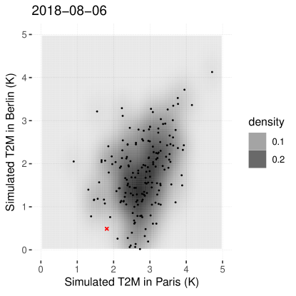
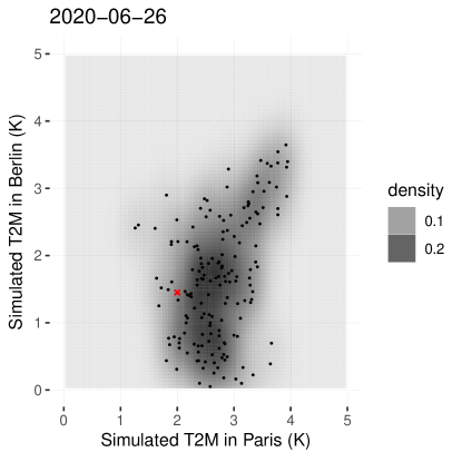
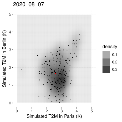
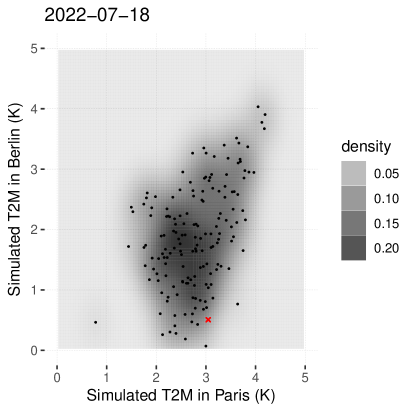
Figure 4: Two-dimensional density plots of T2M values at two grid points (containing Paris in the x-axes and Berlin in the y-axes) from 200 model simulations (black dots) on various heat extreme days (represented by the different panels) in the test set, conditional on positive T2M values and an $r$-exceedance. The red crosses represent the realised T2M from the ERA5 reanalysis.

Figure 4 showcases 200 model simulations across four distinct heat extreme days for two grid points in central Europe: Berlin and Paris. The realised T2M at both grid points on all days are within the range of the other heat events generated by the model. In terms of process understanding, these simulations suggest that other spatially dependent heat extremes with jointly large T2M values at multiple locations are possible. This illustrates the strength of our theoretically-justified approach to extrapolate beyond the range of observed data with plausible spatial extremal dependencies.

To evaluate our models performance, we compare our predictions to ERA5 on the test set (2018–2022). Notably, the Z500 predictors substantially improves predictive performance. The occurrence sub-model obtains an impressive area under the curve score (AUC) of 0.899, and its Receiver Operating Curve (ROC) is displayed in Figure 5. For the intensity sub-model, Figure 6 highlights a good overall fit to the local empirical tail distribution for an $r$-exceedance at four selected grid points containing Berlin, London, Barcelona and Paris. The improvement in predictive skill when modeling spatial dependence in extremes is further highlighted in the SI.

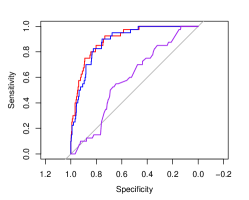
Figure 5: ROC for the occurrence sub-models on the test set (2018–2022). Displayed are the curves corresponding to the model without the SM predictor (blue), without the Z500 predictor (purple), and the full model (red). The curve closer to the top left corner (and away from the diagonal) is better. The Area under the Curve (AUC) scores are 0.589, 0.885 and 0.899, respectively.

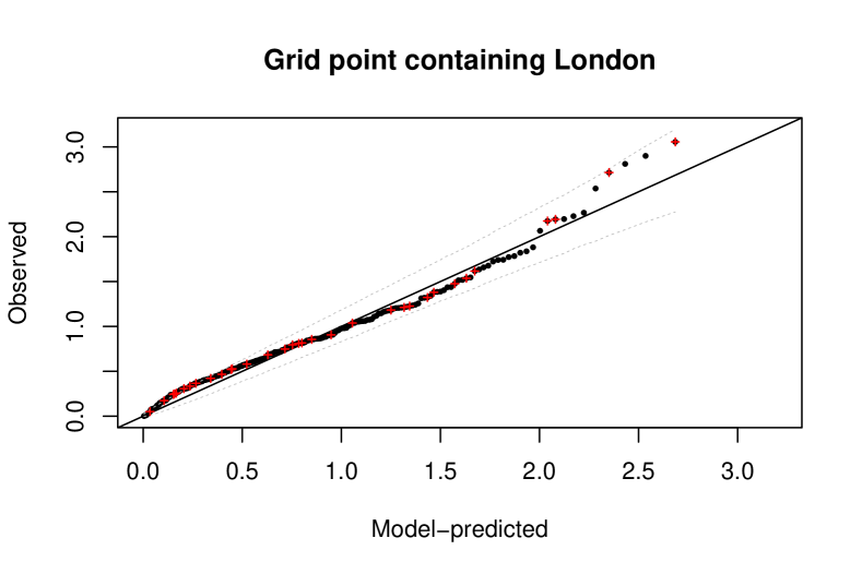
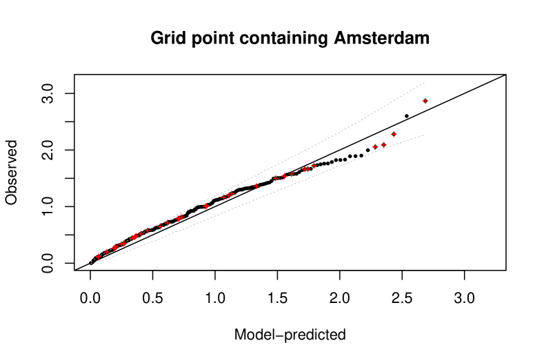
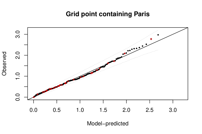
Figure 6: Quantile-Quantile plots comparing the intensity model’s scaled tail distributional prediction above $b_{d}$ given an $r$-exceedance (x-axes), with that from ERA5 (y-axes), for four chosen grid points $d$ and on both the training (black dots) and test sets (red crosses). The dashed lines correspond to $95\%$ pointwise parametric bootstrap confidence intervals.

Importance of Z500 large-scale weather patterns

We use the predictions from our model to identify key features of the large-scale weather patterns that favor the formation of European heat extremes. We perform a composite analysis to investigate the underlying mechanisms related to the two predictor fields Z500 and SM.

We first analyze composite maps of the predictor field Z500 anomaly conditioned on when the sub-models predicted high values (the top 10% of the values) of the occurrence probabilities, the intensities, and the spatial dependence of the heat extremes. Furthermore, Shapley additive explanations (SHAP; 69) values give a measure of the contribution of each Z500 predictor to the final outcome of each sub-model. These approaches provide prediction-level interpretation (70) of our models.

The Z500 anomalies (here, averaged over the previous 5 days) associated with the top 10% of values in all sub-models (Figure 7A,D,G) show anticyclonic anomalies (exceeding 1.5 standard deviations) over the target region that are part of a large-scale wave pattern. This wave pattern includes an upstream trough over the Atlantic ocean and a weaker downstream trough over eastern Europe. Anticyclonic anomalies favor subsidence, leading to adiabatic heating and cloud-free skies associated with absence of precipitation. In addition, the upstream trough can contribute to horizontal warm air advection at the upstream flank of the anticyclone (e.g., 30, 71).

Comparing the composites for occurrence probability, intensity, and spatial dependence, we note differences in the relative position, the intensity and the shape of the anticyclone and troughs across these composites. For the occurrence model (Figure 7A), the trough to the south of the anticyclone over the Mediterranean indicates the presence of a dipole block pattern, favoring the stagnation of the large-scale flow (72). The SHAP in Figure 7C highlights the center of the anticyclone and the region upstream over the North Atlantic as important - emphasizing the importance of both the local and the upstream circulation patterns for heat extreme occurrence. For the intensity model (Figure 7D,F), the anticyclone appears more elongated in a meridional direction and is flanked by upstream and downstream troughs, resembling more an omega blocking pattern. The SHAP analysis does not highlight a specific area within the block, but rather suggests that the heat intensity is influenced by the entire trough-ridge pattern across the Euro-Atlantic region. For the spatial dependence model (Figure 7G), the Z500 composite shows a broader ridge pattern with a anticyclone that is less intense than those in other composites. The SHAP analysis (Figure 7I) draws attention to the anticyclone’s flanks, underscoring the zonal extent of the block, rather than its core, as important in driving spatially extensive heat extremes.

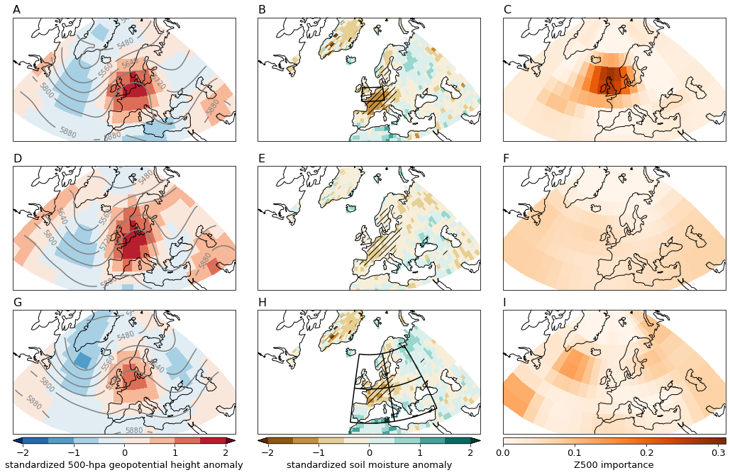
Figure 7: Composite maps of five-day averaged standardized Z500 anomaly (color shading), absolute Z500 contours (grey lines)(A,D,G), and maps of 15-day averaged SM anomaly and standardized T2m anomaly (hatching for areas with $>+1$ STD) (B,E,H) for the 10% heat extremes with highest predicted occurrence probabilities (first row), intensity (second row), and spatial dependence (third row). Variable importance plots (with kernel density spatial smoothing) of the top Z500 predictors with the region averaged SHAP metric, for the models predicting: (C) $\theta^{\mathrm{prod}}$, (F) $\theta^{\mathrm{int}}$ and (I) $\theta^{\mathrm{extent}}$.

Importance of soil moisture

SM anomalies emerge as a salient predictor across our models, albeit with varying impacts on the performance. SM anomalies align well with the Z500 composites, particularly in their spatial distribution: SM is depleted beneath the anticyclone (Figure 7B,E,H).

In the occurrence sub-model, SM averaged over the target region ranks sixth in importance among 243 predictors based on SHAP values. Beneath the anticyclone, SM is notably depleted (more than -1 standard deviations away from the 1991–2020 climate, Figure 7B), implying that (pre-conditioning) soil dryness (in our case, over the last 15 days) is favourable for heat extremes, in accordance with the literature (e.g., 33, 39). Model performance, as evidenced by the ROC, improves slightly with the SM predictor in the test set (Figure 5), though the role of the Z500 predictors still dominates.

For the intensity sub-model, the local SM at a specific grid point appears as the top three most important predictor (along with latitude and longitude). SM is depleted in the target region (Figure 7E), albeit less compared to the occurrence sub-model’s composite map. Unlike before, however, the inclusion of the SM predictor does not significantly improve test error, as measured by the Generalized Pareto Distribution (GPD) loss likelihood. This suggests that extreme heat intensities can be simulated from our model just as accurately without SM information.

In the spatial dependence sub-model, SM is depleted below the anticyclone, but not in its surrounding areas, as shown in Figure 7H. The predictor corresponding to the average SM over the United Kingdom (top left region of our study region) appears in the top 10 spatial dependence sub-model, though as before, the predictive improvement of having the SM related predictors is small.

Conclusion

A key ingredient of machine learning models is the loss function used for training, and choices for these functions in climate sciences have largely been restricted to those that emphasise good prediction of the distributional bulk instead of the tails. For example, the root mean squared error, the default for modelling real-valued responses in many applications, implicitly presupposes that the target of interest is the conditional mean given the predictors, which may be inappropriate if the focus is on extreme values. We here introduce a new approach for modelling spatially compounding weather extremes that focuses specifically on the distributional tails of the data. Our approach uniquely employs loss functions motivated by spatial EVT to train ML models to assess daily extreme weather events, very importantly including their spatial dependencies. Unlike traditional approaches that employ summary metrics of Z500 spatial patterns, such as EOF-derived weather regimes (50, 73) or selected regional averages, our approach leverages high-spatiotemporal-resolution predictors to model the functional exceedances across spatial fields. Applied here to the study of heat extremes in western Europe, this allows for a more granular understanding of the large-scale processes associated with of their occurrence, intensity, and spatial dependencies.

Another important feature of our approach is the ability to extrapolate beyond the range of the observational record, not just in terms of the magnitude but also regarding the spatial extent of extreme events. We showcase this with our case study of using the model to generate counterfactual extreme heat events in our test set. Our approach provides an alternative to physical model-based techniques or other ML models, and sets a solid foundation for future work with this feature, e.g., it can provide a valuable tool for impact modelling.

For model validation, we use daily gridded data from the ECMWF ERA5 reanalysis, recognizing that the limited duration of observational records presents challenges for extreme value theory analysis and evaluating tail properties in the data distribution. Future work may therefore consider leveraging long-term climate simulations (e.g., as done in 74, 75), to obtain more robust model validation.

Our predictors capture persistence and pre-conditions, as they are averaged over the previous 5 days (Z500) or 15 days (SM). We choose these predictors based on plausible physical mechanisms known to contribute to heat extremes. Our model elucidates the large-scale weather patterns conducive to heat extremes in Western Europe. Heat extremes in Europe are closely linked to Z500 anomalies of the atmospheric circulation with intense (blocking) anticyclones and upstream and downstream troughs. (Blocking) anticyclones provide a condition favorable for the build-up of high temperature over the study region (e.g., 26, 27). Anticyclones extending farther north are found to concentrate intense heat over a more localized region, while broad ridges result in widespread heat extremes. We find that upstream and downstream troughs are also important in modulating the intensity and spatial extent of heat extremes (76, 77). Pronounced dry soils beneath the (blocking) anticyclone prior to the heat extremes are important for the occurrence of heat extremes, which has been documented for previous heatwaves in Europe (e.g., 35). However, its importance as precursor for the intensity of heat extremes is less clear.

This work motivates new avenues of research using ML tools to fit new theoretically-motivated models for extreme values. This includes, but is not limited to, varying types of extremes, regions of interest, predictor sets, and even the types of machine learning models deployed. Another related avenue is to use our framework to improve on numerical weather prediction or sub-seasonal to seasonal prediction models, serving as an advanced post-processing tool.

The authors gratefully acknowledge support from Johanna Ziegel, the Oeschger Centre for Climate Change Research and the Wyss Academy for Nature, University of Bern.

blabla

blabla

Supporting Information Appendix (SI)

Simulation study

We simulate a Brown-Resnick model with the same number of $r$-exceedance times and grid points as in our study, with $\alpha=1$ and $\theta=0$ for all $t\in\mathcal{T}$, while ${\theta}^{\text{extent}}_{t}$ depend only a few predictors in a non-linear way. We however still use all predictors when training the model to examine if our learning procedure can discriminate the signal from the noise.

We predict all the parameters for 100 independent replicates of this model. Figure 8 suggests that the trend is already well detected with $272$ $r$-exceedances, and the joint probabilities of exceedance estimates are generally unbiased with $42\%$ of the truth falling within the interquantile ranges of the boxplots. The empirical variance tends to be larger for the ones associated with higher joint probabilities; this is consistent with previous studies that found that the parameters associated with higher spatial extended events tend to be harder to estimate (e.g., 78).

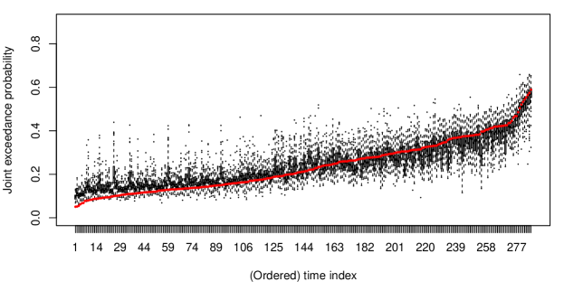
Figure 8: Boxplots for $\hat{\pi}_{t}(\bm{s}_{1},\bm{s}_{2})$ in our simulation study after 190 boosting iterations, where $\bm{s}_{1}$ is the location of London and $\bm{s}_{2}$ of Barcelona. The red dots represent the truth.

Boosting hyperparameters and cross validation

We choose the maximum depth of the trees used in all our sub-models to be between $5$ to $8$. Our boosting algorithm is based on approximate algorithm with weighted quantile sketch in xgboost; for more details see (59, , Appendix A). Figure 9 shows the five-fold cross validation results from the dependence and intensity sub-models. For the intensity sub-model, $\xi=-0.3$ was chosen because the cross validation curve corresponding to that setting gave the lowest score.

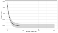
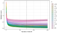
Figure 9: The average rescaled evaluation score across a random five-fold cross-validation scheme for the (left) dependence model using $\mathcal{L}_{\text{GrP}}$ to predict $\hat{\theta}_{t}^{\mathrm{extent}}$, and (right) the intensity model that uses $\mathcal{L}_{\text{GPD}}$ to predict $\hat{\theta}_{d,t}^{\mathrm{int}}$. The shaded regions shows the pointwise one-standard-error bound. The dotted lines pinpoints the number of trees chosen by the one-standard-error rule.

Added value of the spatial sub-model

We now compare our proposed spatial sub-model that has spatial extremal dependence varying with predictors, with another that assumes spatial extremal independence throughout the study region; the latter uses only the intensity sub-model, and reflects the common practice used in the climate extremes literature when modelling peaks-over-threshold data, e.g., when the GPD is used to model excesses over a high threshold at each location separately.

Using the average Brier score (79), we evaluate and compare the models’ ability to predict joint exceedances above various local empirical quantiles of T2M from the 40 $r$-exceedance days in the test set at two grid points, using the conditional probability (3), with $q$ the chosen quantile. The severity thresholds are chosen low enough to retain enough observations to evaluate these scores with sufficient precision, but sufficiently high for extreme risk assessment. Note that the thresholds indicated are the grid point-wise empirical quantiles from the $272$ $r$-exceedance days from the training set and not from the full dataset; the quantile of $0.4$ in the grid point containing Paris, for example, corresponds to a high of $+2.2$K.

Table 1 shows good relative performance of our sub-model throughout. To better grasp the uncertainty in scores, we calculate p-values of a permutation test assessing the differences in scores based on 10’000 permutations. The score differences’ uncertainty increases for higher thresholds as the score is averaged over fewer observations, though the scores for our spatial model are always better or equal to the other model. This illustrates the benefits of modelling the spatial dependence in the extremes, though some of the high p-values indicate that a validation dataset with a longer observational record would be beneficial, as we are considering only $40$ $r$-exceedance days from the test set. Evaluating models for very extreme events is always challenging, especially with varying spatial dependence; this is an avenue for future research.

	Q40/Q50/Q60/Q70
Model	London	Paris	Berlin	Amsterdam
Spatial	28/25/20/11	28/27/26/16	27/28/25/26	34/34/33/26
Independent	34/30/23/11	37/35/34/18	36/36/32/33	39/39/39/29
p-val	20/28/38/48	14/21/24/41	16/22/28/27	21/28/30/36

Table 1: Mean Brier score calculated from the ERA5 test set (2018-2022) by comparing the observed 0-1 indicators for the joint exceedance at grid point $\bm{s}_{1}$ and $\bm{s}_{2}$ conditional on an $r$-exceedance, against the model-estimated joint probabilities. The empirical quantiles from the $r$-exceedance days are $q=\{0.4,0.5,0.6,0.7\}$, separated in each cell of the table by “/”. The grid point $\bm{s}_{1}$ corresponds to the grid points containing London, Paris, Berlin or Amsterdam, and $\bm{s}_{2}$ to a randomly sampled grid point neighbouring $\bm{s}_{1}$. P-values ($\times 10^{2}$) are calculated from permutation tests where the alternative hypotheses are that the spatial model does better. A lower score is better.

Code for loss functions and boosting algorithm

Code to run the methods outlined in the Methods and models section, along with data files to reproduce the data analysis is available upon request. The full code will be made available in the form of an R package EVTxgboost, documented with a step-by-step tutorial, latest before journal publication.

References

- (1) K Kornhuber, et al., Amplified Rossby waves enhance risk of concurrent heatwaves in major breadbasket regions. \JournalTitleNature Climate Change 10, 48–53 (2020).
- (2) J Zscheischler, SI Seneviratne, Dependence of drivers affects risks associated with compound events. \JournalTitleScience Advances 3, e1700263 (2017).
- (3) J Zscheischler, et al., A typology of compound weather and climate events. \JournalTitleNature Reviews Earth & Environment 1, 333–347 (2020).
- (4) D Coumou, S Rahmstorf, A decade of weather extremes. \JournalTitleNature Climate Change 2, 491–496 (2012).
- (5) MM Vogel, J Zscheischler, R Wartenburger, D Dee, SI Seneviratne, Concurrent 2018 Hot Extremes Across Northern Hemisphere Due to Human-Induced Climate Change. \JournalTitleEarth’s Future 7, 692–703 (2019).
- (6) AM Vicedo-Cabrera, et al., The burden of heat-related mortality attributable to recent human-induced climate change. \JournalTitleNature Climate Change 11, 492–500 (2021).
- (7) RH White, et al., The unprecedented Pacific Northwest heatwave of June 2021. \JournalTitleNature Communications 14, 727 (2023).
- (8) C Schär, et al., The role of increasing temperature variability in European summer heatwaves. \JournalTitleNature 427, 332–336 (2004).
- (9) M Matsueda, Predictability of Euro-Russian blocking in summer of 2010. \JournalTitleGeophysical Research Letters 38 (2011).
- (10) D Barriopedro, EM Fischer, J Luterbacher, RM Trigo, R García-Herrera, The Hot Summer of 2010: Redrawing the Temperature Record Map of Europe. \JournalTitleScience 332, 220–224 (2011).
- (11) S Russo, J Sillmann, EM Fischer, Top ten European heatwaves since 1950 and their occurrence in the coming decades. \JournalTitleEnvironmental Research Letters 10, 124003 (2015).
- (12) M Drouard, K Kornhuber, T Woollings, Disentangling Dynamic Contributions to Summer 2018 Anomalous Weather Over Europe. \JournalTitleGeophysical Research Letters 46, 12537–12546 (2019).
- (13) E Rousi, et al., The extremely hot and dry 2018 summer in central and northern Europe from a multi-faceted weather and climate perspective. \JournalTitleEGUsphere pp. 1–37 (2022).
- (14) D Mitchell, K Kornhuber, C Huntingford, P Uhe, The day the 2003 European heatwave record was broken. \JournalTitleThe Lancet Planetary Health 3, e290–e292 (2019).
- (15) O Lhotka, J Kyselý, The 2021 European Heat Wave in the Context of Past Major Heat Waves. \JournalTitleEarth and Space Science 9, e2022EA002567 (2022).
- (16) D Faranda, S Pascale, B Bulut, Persistent anticyclonic conditions and climate change exacerbated the exceptional 2022 European-Mediterranean drought. \JournalTitleEnvironmental Research Letters (2023).
- (17) T Kelder, et al., Using unseen trends to detect decadal changes in 100-year precipitation extremes. \JournalTitlenpj Climate and Atmospheric Science 3, 47 (2020).
- (18) C Gessner, EM Fischer, U Beyerle, R Knutti, Very rare heat extremes: Quantifying and understanding using ensemble reinitialization. \JournalTitleJournal of Climate 34, 6619–6634 (2021).
- (19) EM Fischer, et al., Storylines for unprecedented heatwaves based on ensemble boosting. \JournalTitleNature Communications 14, 4643 (2023).
- (20) J Pathak, et al., Fourcastnet: A global data-driven high-resolution weather model using adaptive fourier neural operators (2022).
- (21) K Bi, et al., Accurate medium-range global weather forecasting with 3d neural networks. \JournalTitleNature (2023).
- (22) R Lam, et al., Learning skillful medium-range global weather forecasting. \JournalTitleScience 0, eadi2336 (2023).
- (23) M Chantry, ZB Bouallegue, L Magnusson, M Maier-Gerber, J Dramsch, The rise of machine learning in weather forecasting (https://www.ecmwf.int/en/about/media-centre/science-blog/2023/rise-machine-learning-weather-forecasting) (2023) Accessed: 2023-07-20.
- (24) AC Davison, SA Padoan, M Ribatet, Statistical modeling of spatial extremes. \JournalTitleStatistical Science 27, 161–186 (2012).
- (25) R Huser, JL Wadsworth, Advances in statistical modeling of spatial extremes. \JournalTitleWIREs Computational Statistics 14, e1537 (2022).
- (26) M Röthlisberger, L Papritz, Quantifying the physical processes leading to atmospheric hot extremes at a global scale. \JournalTitleNature Geoscience pp. 1–7 (2023).
- (27) D Barriopedro, R García-Herrera, C Ordóñez, DG Miralles, S Salcedo-Sanz, Heat Waves: Physical Understanding and Scientific Challenges. \JournalTitleReviews of Geophysics 61, e2022RG000780 (2023).
- (28) S Pfahl, H Wernli, Quantifying the relevance of atmospheric blocking for co-located temperature extremes in the Northern Hemisphere on (sub-)daily time scales. \JournalTitleGeophysical Research Letters 39 (2012).
- (29) PM Sousa, et al., Responses of European precipitation distributions and regimes to different blocking locations. \JournalTitleClimate Dynamics 48, 1141–1160 (2017).
- (30) LA Kautz, et al., Atmospheric blocking and weather extremes over the Euro-Atlantic sector – a review. \JournalTitleWeather and Climate Dynamics 3, 305–336 (2022).
- (31) L Suarez-Gutierrez, WA Müller, C Li, J Marotzke, Dynamical and thermodynamical drivers of variability in European summer heat extremes. \JournalTitleClimate Dynamics 54, 4351–4366 (2020).
- (32) DIV Domeisen, et al., Prediction and projection of heatwaves. \JournalTitleNature Reviews Earth & Environment 4, 36–50 (2023).
- (33) EM Fischer, SI Seneviratne, PL Vidale, D Lüthi, C Schär, Soil Moisture–Atmosphere Interactions during the 2003 European Summer Heat Wave. \JournalTitleJournal of Climate 20, 5081–5099 (2007).
- (34) SI Seneviratne, D Lüthi, M Litschi, C Schär, Land–atmosphere coupling and climate change in Europe. \JournalTitleNature 443, 205–209 (2006).
- (35) SI Seneviratne, et al., Investigating soil moisture–climate interactions in a changing climate: A review. \JournalTitleEarth-Science Reviews 99, 125–161 (2010).
- (36) PM Sousa, et al., Distinct influences of large-scale circulation and regional feedbacks in two exceptional 2019 European heatwaves. \JournalTitleCommunications Earth & Environment 1, 1–13 (2020).
- (37) Y Zhang, WR Boos, An upper bound for extreme temperatures over midlatitude land. \JournalTitleProceedings of the National Academy of Sciences 120, e2215278120 (2023).
- (38) A Tuel, O Martius, On the persistence of warm and cold spells in the Northern Hemisphere extratropics: Regionalisation, synoptic-scale dynamics, and temperature budget. \JournalTitleEGUsphere pp. 1–36 (2023).
- (39) DG Miralles, AJ Teuling, CC van Heerwaarden, J Vilà-Guerau de Arellano, Mega-heatwave temperatures due to combined soil desiccation and atmospheric heat accumulation. \JournalTitleNature Geoscience 7, 345–349 (2014).
- (40) K Wehrli, BP Guillod, M Hauser, M Leclair, SI Seneviratne, Identifying Key Driving Processes of Major Recent Heat Waves. \JournalTitleJournal of Geophysical Research: Atmospheres 124, 11746–11765 (2019).
- (41) P Xu, L Wang, P Huang, W Chen, Disentangling dynamical and thermodynamical contributions to the record-breaking heatwave over Central Europe in June 2019. \JournalTitleAtmospheric Research 252, 105446 (2021).
- (42) RM Horton, JS Mankin, C Lesk, E Coffel, C Raymond, A Review of Recent Advances in Research on Extreme Heat Events. \JournalTitleCurrent Climate Change Reports 2, 242–259 (2016).
- (43) J Koh, Gradient boosting with extreme–value theory for wildfire prediction. \JournalTitleExtremes 26, 273–299 (2023).
- (44) J Velthoen, C Dombry, JJ Cai, S Engelke, Gradient boosting for extreme quantile regression. \JournalTitleExtremes 26, 639–667 (2023).
- (45) N Gnecco, EM Terefe, S Engelke, Extremal random forests. \JournalTitlearXiv preprint:2201.12865 (2022).
- (46) J Richards, R Huser, Regression modelling of spatiotemporal extreme U.S. wildfires via partially-interpretable neural networks. \JournalTitlearXiv preprint:2208.07581 (2022).
- (47) OC Pasche, S Engelke, Neural networks for extreme quantile regression with an application to forecasting of flood risk. \JournalTitlearXiv preprint:2208.07590 (2022).
- (48) R de Fondeville, AC Davison, Functional peaks-over-threshold analysis. \JournalTitleJournal of the Royal Statistical Society Series B: Statistical Methodology 84, 1392–1422 (2022).
- (49) BM Brown, SI Resnick, Extreme values of independent stochastic processes. \JournalTitleJournal of Applied Probability 14, 732–739 (1977).
- (50) CM Grams, R Beerli, S Pfenninger, I Staffell, H Wernli, Balancing Europe’s wind-power output through spatial deployment informed by weather regimes. \JournalTitleNature Climate Change 7, 557–562 (2017).
- (51) JH Friedman, Greedy function approximation: a gradient boosting machine. \JournalTitleAnnals of Statistics 29, 1189–1232 (2001).
- (52) H Hersbach, et al., The era5 global reanalysis. \JournalTitleQuarterly Journal of the Royal Meteorological Society 146, 1999–2049 (2020).
- (53) SE Perkins, A review on the scientific understanding of heatwaves—Their measurement, driving mechanisms, and changes at the global scale. \JournalTitleAtmospheric Research 164–165, 242–267 (2015).
- (54) SE Perkins-Kirkpatrick, SC Lewis, Increasing trends in regional heatwaves. \JournalTitleNature Communications 11, 3357 (2020).
- (55) AC Davison, RL Smith, Models for exceedances over high thresholds (with discussion). \JournalTitleJournal of the Royal Statistical Society: Series B (Methodological) 52, 393–442 (1990).
- (56) C Dombry, M Ribatet, Functional regular variations, Pareto processes and peaks over thresholds. \JournalTitleStatistics and Its Interface 8, 9–17 (2015).
- (57) S Engelke, AS Hitz, Graphical Models for Extremes (with discussion). \JournalTitleJournal of the Royal Statistical Society Series B: Statistical Methodology 82, 871–932 (2020).
- (58) B Greenwell, B Boehmke, J Cunningham, G Developers, gbm: Generalized Boosted Regression Models, (2020) R package version 2.1.8.
- (59) T Chen, C Guestrin, XGBoost: a scalable tree boosting system in Proceedings of the 22nd ACM SIGKDD International Conference on Knowledge Discovery and Data Mining, KDD ’16. (ACM, New York, NY, USA), pp. 785–794 (2016).
- (60) CS Bojer, JP Meldgaard, Kaggle forecasting competitions: An overlooked learning opportunity. \JournalTitleInternational Journal of Forecasting 37, 587–603 (2021).
- (61) L Breiman, JH Friedman, RA Olshen, CJ Stone, Classification and Regression Trees. (Wadsworth and Brooks, Monterey, CA), (1984).
- (62) JH Friedman, Contrast trees and distribution boosting. \JournalTitleProceedings of the National Academy of Sciences 117, 21175–21184 (2020).
- (63) J Friedman, T Hastie, R Tibshirani, Additive logistic regression: a statistical view of boosting (with discussion and a rejoinder by the authors). \JournalTitleThe Annals of Statistics 28, 337–407 (2000).
- (64) A Hyvärinen, Some extensions of score matching. \JournalTitleComputational Statistics & Data Analysis 51, 2499–2512 (2007).
- (65) S Engelke, A Malinowski, Z Kabluchko, M Schlather, Estimation of Huesler-Reiss distributions and Brown-Resnick processes. \JournalTitleJournal of the Royal Statistical Society: Series B (Statistical Methodology) 77, 239–265 (2015).
- (66) A Hyvärinen, Estimation of non-normalized statistical models by score matching. \JournalTitleJournal of Machine Learning Research 6, 695–709 (2005).
- (67) AV Vecchia, Estimation and model identification for continuous spatial processes. \JournalTitleJournal of the Royal Statistical Society. Series B (Methodological) 50, 297–312 (1988).
- (68) J Guinness, Permutation and grouping methods for sharpening gaussian process approximations. \JournalTitleTechnometrics 60, 415–429 (2018) PMID: 31447491.
- (69) SM Lundberg, GG Erion, SI Lee, Consistent individualized feature attribution for tree ensembles. \JournalTitlearXiv preprint:1802.03888 (2019).
- (70) WJ Murdoch, C Singh, K Kumbier, R Abbasi-Asl, B Yu, Definitions, methods, and applications in interpretable machine learning. \JournalTitleProceedings of the National Academy of Sciences 116, 22071–22080 (2019).
- (71) A Tuel, O Martius, On the persistence of warm and cold spells in the northern hemisphere extratropics: regionalisation, synoptic-scale dynamics, and temperature budget. \JournalTitleEGUsphere 2023, 1–36 (2023).
- (72) DF Rex, Blocking Action in the Middle Troposphere and its Effect upon Regional Climate. \JournalTitleTellus 2, 196–211 (1950).
- (73) E Rouges, L Ferranti, H Kantz, F Pappenberger, European heatwaves: Link to large-scale circulation patterns and intraseasonal drivers. \JournalTitleInternational Journal of Climatology 43, 3189–3209 (2023).
- (74) F Ragone, J Wouters, F Bouchet, Computation of extreme heat waves in climate models using a large deviation algorithm. \JournalTitleProceedings of the National Academy of Sciences 115, 24–29 (2018).
- (75) J Zeder, S Sippel, OC Pasche, S Engelke, EM Fischer, The Effect of a Short Observational Record on the Statistics of Temperature Extremes. \JournalTitleGeophysical Research Letters 50, e2023GL104090 (2023).
- (76) D Steinfeld, M Boettcher, R Forbes, S Pfahl, The sensitivity of atmospheric blocking to upstream latent heating – numerical experiments. \JournalTitleWeather and Climate Dynamics 1, 405–426 (2020).
- (77) E Neal, CSY Huang, N Nakamura, The 2021 Pacific Northwest Heat Wave and Associated Blocking: Meteorology and the Role of an Upstream Cyclone as a Diabatic Source of Wave Activity. \JournalTitleGeophysical Research Letters 49, e2021GL097699 (2022).
- (78) H Sang, MG Genton, Tapered composite likelihood for spatial max-stable models. \JournalTitleSpatial Statistics 8, 86–103 (2014).
- (79) GW Brier, Verification of forecasts expressed in terms of probability. \JournalTitleMonthly Weather Review 78, 1–3 (1950).