Supplemental Material: Yielding is an absorbing phase transition with vanishing critical fluctuations

I Determination of the yield stress

To perform our finite-size scaling analysis, it is crucial to get a precise measurement of $\Sigma_{\mathrm{y}}$. To do so we first measure the flow curve. For the short-range models SR-Picard and FES^±, this is done by running simulations at different constant shear stresses $\Sigma$, measuring $\langle\dot{\gamma}\rangle$. For the Picard model, the fact that the transition is convex makes it more difficult to get close to the critical point without falling into an absorbing state. To overcome this issue, we change the control parameter and drive our system at a constant shear rate $\dot{\gamma}$, and measure $\langle\Sigma\rangle$. In all cases, once we determine the flow curve, $\Sigma_{\mathrm{y}}$ is adjusted to get a power law close to the transition, $\langle\dot{\gamma}\rangle=f(\Sigma-\Sigma_{\mathrm{y}})\sim(\Sigma-\Sigma_{\mathrm{y}})^{\beta}$ (or accordingly $\dot{\gamma}=f(\langle\Sigma\rangle-\Sigma_{\mathrm{y}})$), as can be seen in Fig. 1. Along with $\Sigma_{\mathrm{y}}$, we also obtain $\beta$.

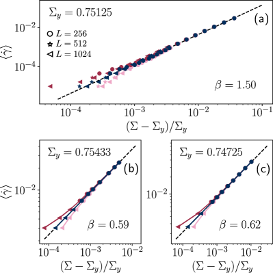
Figure 1: Stress-strain curves for the determination of the critical yield stress $\Sigma_{y}$ in the Picard (a), SR-Picard (b) and $\text{FES}^{\pm}$ (c) model. Blue curves correspond to $\Sigma_{y}$, pink to $\Sigma_{y}-5\times 10^{-5}$ and red to $\Sigma_{y}+5\times 10^{-5}$.

II Finite-size scaling analysis

For an infinite system, in the critical regime the order parameter and its fluctuations are homogeneous functions of the distance to the critical point $\delta\Sigma$ and of the activation field $h$, that is,

$$\langle\dot{\gamma}\rangle \sim\lambda^{-\beta}R(a_{\Sigma}\lambda\delta\Sigma,a_{h}\lambda^{\zeta}h)\,,$$ (1)

$$a_{\Delta}N(\Delta\dot{\gamma})^{2} \sim\lambda^{\gamma^{\prime}}D(a_{\Sigma}\lambda\delta\Sigma,a_{h}\lambda^{\zeta}h)\,,$$

for any $\lambda\in\mathbb{R}$, with $a_{\Sigma,h,\Delta}$ non-universal coefficients. If we impose the system to be at the critical stress $\Sigma_{\mathrm{y}}$ and take $\lambda=(a_{h}h)^{-1/\zeta}$ we get

$$\langle\dot{\gamma}\rangle \sim(a_{h}h)^{\beta/\zeta}R(0,1)\,,$$ (2)

$$a_{\Delta}N(\Delta\dot{\gamma})^{2} \sim(a_{h}h)^{-\gamma^{\prime}/\zeta}D(0,1)\,.$$

However, for systems with finite size $L$, we get deviations from these power laws, as finite-size effects occur when the diverging correlation length becomes comparable to the system size, as can be seen in Fig. 2. Finite-size effects can be taken into account by modifying the scaling functions dependency as [1]

$$\langle\dot{\gamma}\rangle \sim\lambda^{-\beta}\tilde{R}(a_{\Sigma}\lambda\delta\Sigma,a_{h}\lambda^{\zeta}h,a_{L}L\lambda^{-\nu_{\perp}})\,,$$ (3)

$$a_{\Delta}N(\Delta\dot{\gamma})^{2} \sim\lambda^{\gamma^{\prime}}\tilde{D}(a_{\Sigma}\lambda\delta\Sigma,a_{h}\lambda^{\zeta}h,a_{L}L\lambda^{-\nu_{\perp}})\,.$$

Taking $\Sigma=\Sigma_{\mathrm{y}}$ and $\lambda=(a_{L}L)^{1/\nu_{\perp}}$ we get:

$$\langle\dot{\gamma}\rangle \sim(a_{L}L)^{-\beta/\nu_{\perp}}\tilde{R}(0,a_{h}(a_{L}L)^{\zeta/\nu_{\perp}}h,1),$$ (4)

$$a_{\Delta}N(\Delta\dot{\gamma})^{2} \sim(a_{L}L)^{\gamma^{\prime}/\nu_{\perp}}\tilde{D}(0,a_{h}(a_{L}L)^{\zeta/\nu_{\perp}}h,1).$$

In other words, all curves for different system sizes should collapse under the rescaling:

$$h \rightarrow hL^{\zeta/\nu_{\perp}},$$ (5)

$$\langle\dot{\gamma}\rangle \rightarrow\langle\dot{\gamma}\rangle L^{\beta/\nu_{\perp}},$$

$$(\Delta\dot{\gamma})^{2} \rightarrow(\Delta\dot{\gamma})^{2}L^{-\gamma^{\prime}/\nu_{\perp}}.$$

This then represents an efficient way to determine all the exponents associated with the transition. To further constrain the exponent values, we also perform FSS on the fourth-order cumulant $Q$ defined as [2]

$$Q=1-\frac{\langle\dot{\gamma}^{4}\rangle}{3\langle\dot{\gamma}^{2}\rangle^{2}}$$ (6)

whose associated curves should collapse only under the rescaling of the activation field $h$. This first collapse allows us to determine the exponents ratio $\zeta/\nu_{\perp}$. Then the collapse of the mean value determines $\beta/\nu_{\perp}$ which directly determines $\nu_{\perp}$ since $\beta$ is known from the critical stress determination. Finally $\gamma^{\prime}/\nu_{\perp}$ is extracted from the collapse of the variance from which we get $\gamma^{\prime}$. The hyperscaling relation is tested a posteriori and is not used to determine any exponent.

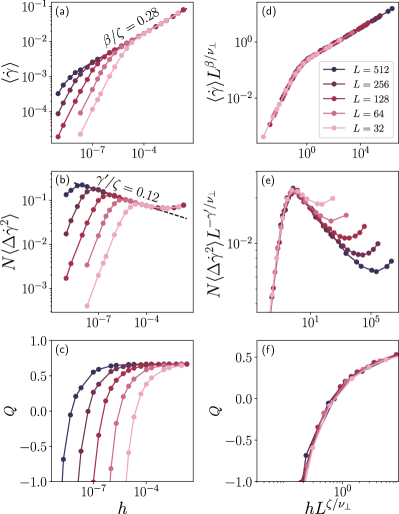
Figure 2: Finite-size scaling analysis of the SR-Picard model. Left: raw data for the mean shear rate (a), its variance (b) and its fourth order cumulant (c). Right: rescaled data (d-f) with the set of critical exponents $(\beta=0.59,\gamma^{\prime}=0.26,\nu_{\perp}=0.70,\zeta=2.10)$

III CDP test for SR-Picard and FES^± models

In this section we test whether the SR-Picard and FES^± are compatible with the CDP universality class. For this, we rescale the data using the CDP exponents $(\beta,\zeta,\gamma^{\prime},\nu_{\perp})$ and assess if we get a good collapse. Results are shown on Fig. 3. For the SR-Picard the collapse is significantly worse than the one we obtained in Fig. 2 with non-CDP exponents, which supports that the SR-Picard does not belong to the CDP class. By contrast, for the FES^± the collapse using CDP exponents is as good as the one we performed in Fig. 2 using freely adjusted exponents that turned out to be very close to the CDP ones, supporting that FES^± belongs to the CDP class.

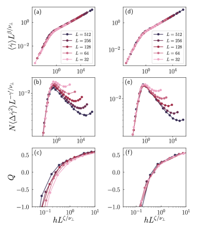
Figure 3: Left: rescaled data (a-c) for the SR-Picard model with CDP exponents . Right: rescaled data (d-f) for the FES^± model with CDP exponents.

IV Dependence on the decay exponent of the stress redistribution kernel

We here show the analysis of the $\alpha$-Picard models interpolating continuously from the SR-Picard model to the Picard model. The $\alpha$-Picard models we consider cover stress redistribution kernels spatially decaying with inverse power laws $\propto 1/r^{\alpha}$. To keep the zero-mode, we define the models in Fourier space as:

$$\hat{G}(\mathbf{q})=-b_{\alpha}\frac{q_{x}^{2}q_{y}^{2}}{q^{6-\alpha}}\,,$$ (7)

with $b_{\alpha}$ a constant chosen so that $\int\mathrm{d}\mathbf{q}\leavevmode\nobreak\ \hat{G}(\mathbf{q})\approx-1$ ($b_{2}=4$) and which corresponds in continuous real space to kernels:

$$\mathcal{G}(r,\theta)=B_{\alpha}\frac{C_{\alpha}+\cos 4\theta}{r^{\alpha}}$$ (8)

with

$$B_{\alpha}=b_{\alpha}\frac{\alpha\Gamma(\alpha/2-2)(\alpha-2)(\alpha-4)(2+\alpha)}{\pi 2^{9-\alpha}\Gamma(3-\alpha/2)}$$ (9)

and

$$C_{\alpha}=\frac{(\alpha-2)(4-\alpha)}{\alpha(2+\alpha)}\,.$$ (10)

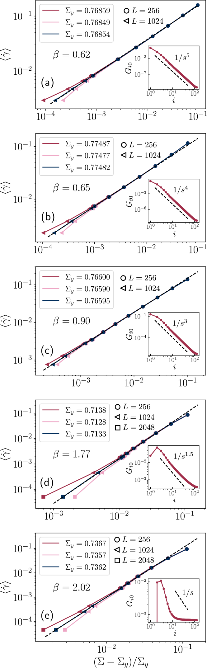
Figure 4: Flow curves for the determination of the critical yield stress $\Sigma_{y}$ in the $\alpha$-Picard models for $\alpha=$ 5(a), 4(b), 3(c), 1.5(d), 1(e). Corresponding discrete propagators in real space are represented in insets.

We determine the critical stress and the associated $\beta$ exponent for $\alpha=\{1,1.5,3,4,5\}$, beside the yielding case ($\alpha=2$) for which we performed full finite-size-scaling analysis. Results are shown in Fig. 4.

V Stress-stress correlations

We start from the general equation on the stress dynamics coupled to the CDP equation for the activity dynamics:

$$\partial_{t}\sigma(\mathbf{r},t) =\left(\mathcal{G}\ast A\right)(\mathbf{r},t)$$ (11)

$$\partial_{t}A(\mathbf{r},t) =(\kappa\sigma(\mathbf{r},t)-\varsigma)A(\mathbf{r},t)-\lambda A^{2}(\mathbf{r},t)+D_{A}\Delta A(\mathbf{r},t)$$

$$+\chi\sqrt{A(\mathbf{r},t)}\eta$$

We then decompose $A(\bm{r},t)=A_{0}+\delta A(\bm{r},t)$ and $\sigma(\bm{r},t)=\sigma_{0}+\delta\sigma(\bm{r},t)$. Linearizing the dynamical equations and taking their spatial and temporal Fourier transforms, we get the correlations of fluctuations:

$$\langle\delta\hat{\sigma}(\bm{q},\omega)\delta\hat{\sigma}(\bm{q}^{\prime},\omega^{\prime})\rangle=\frac{\chi^{2}A_{0}\tilde{\mathcal{G}}(\bm{q})^{2}\delta(\omega+\omega^{\prime})\delta(\bm{q}+\bm{q}^{\prime})}{|\omega^{2}+i\omega(\lambda A_{0}+D_{A}q^{2})+\kappa A_{0}\tilde{\mathcal{G}}(\bm{q})|^{2}}\,.$$ (12)

Keeping in mind that $\tilde{\mathcal{G}}(\bm{q})\leq 0$ in the case of yielding, we integrate this expression on $\omega$ to get the stress correlator in Fourier space at equal times:

$$C_{\tilde{\sigma}\tilde{\sigma}}(\mathbf{q},0)=-\frac{\chi^{2}\tilde{\mathcal{G}}(\bm{q})}{2\kappa(\lambda A_{0}+D_{A}q^{2})}$$ (13)

For a flowing material ($A_{0}>0$), the large scale structure, $q\to 0$ is

$$C_{\tilde{\sigma}\tilde{\sigma}}(\bm{q},0)\underset{q\to 0}{\sim}-\frac{\chi^{2}}{2\kappa}\frac{\tilde{\mathcal{G}}(\bm{q})}{\lambda A_{0}}$$ (14)

which is proportional to $\tilde{\mathcal{G}}(\bm{q})$, as for amorphous solids without applied stress [3] whereas in the quasistatic limit, close to the critical point we get:

$$C_{\tilde{\sigma}\tilde{\sigma}}(\bm{q},0)\underset{A_{0}\to 0}{\sim}-\frac{\chi^{2}}{2\kappa}\frac{\tilde{\mathcal{G}}(\bm{q})}{D_{A}q^{2}}$$ (15)

which is consistent with the fact that the range of correlations should be increased in the critical regime.

VI Relevant terms in the field equation

On the 2D-lattice, the stress evolution for site $(i,j)$ is given by the following discrete convolution:

$$\partial_{t}\sigma_{i,j}=\sum_{k,l}G_{k,l}A_{i-k,j-l}\,.$$ (16)

We then associate the discrete activity and stress fields with their continuous densities:

$$A_{i,j} =\left(\frac{a}{L}\right)^{2}A(x=i\frac{a}{L},y=j\frac{a}{L}),$$ (17)

$$\sigma_{i,j} =\left(\frac{a}{L}\right)^{2}\sigma(x=i\frac{a}{L},y=j\frac{a}{L}),$$

with $a$ the lattice spacing of the square lattice, and $L$ the system size. The evolution equation (16) then becomes:

$$\partial_{t}\sigma(x,y)=\sum_{k,l}G_{k,l}A(x-k\frac{a}{L},y-l\frac{a}{L}).$$ (18)

Considering then that the propagator is short-range enough, the sum in Eq. 18 is restricted to small values of $(k,l)$ so we can expand the activity density

$$A(x-k\frac{a}{L},y-l\frac{a}{L})=\\ \sum_{n,m=0}^{\infty}(-1)^{n+m}\left(\frac{a}{L}\right)^{n+m}\frac{k^{n}l^{m}}{n!m!}\partial_{x}^{n}\partial_{y}^{m}A(x,y)\,.$$ (19)

Keeping in mind that the propagator is 4-fold symmetric and has the zero mode property, only terms involving (strictly) positive and even powers of $k$ and $l$ remain non-zero after the discrete convolution. We thus get:

$$\partial_{t}\sigma(x,y)=\sum_{u,v=1}^{\infty}K_{u,v}\left(\frac{a}{L}\right)^{2(u+v)}\partial_{x}^{2u}\partial_{y}^{2v}A(x,y)\,,$$ (20)

with $K_{u,v}=\sum_{k,l}G_{k,l}\frac{k^{2u}l^{2v}}{(2u)!(2v)!}$. As we take the $a/L\rightarrow 0$ limit to probe large scale behaviors, the relevant field equation to describe this process is:

$$\partial_{t}\sigma(x,y)=\left(\frac{a}{L}\right)^{4}K\partial_{x}^{2}\partial_{y}^{2}A(x,y)\,,$$ (21)

with $K\equiv K_{1,1}$. Using the rescaled time variable $t^{\prime}=t(a/L)^{4}$, Eq. (21) can be recast as

$$\partial_{t^{\prime}}\sigma(x,y)=K\partial_{x}^{2}\partial_{y}^{2}A(x,y)\,.$$ (22)

For long-range propagators $G(r)\sim 1/r^{\alpha}$ we expect this equation to hold for high enough values of $\alpha$. To determine for which $\alpha$ the previous computations do not hold anymore, we go back to Eq. (20). To evaluate the sum on all sites $(k,l)$, we split the propagator into two parts $G=G^{SR}+G^{LR}$. The computations for the short-range part $G^{SR}$ yield the same previous result while for the long-range part we first have to evaluate the sum:

$$\sum_{k,l=1}^{L/a}G_{k,l}^{LR}\frac{k^{2u}l^{2v}}{(2u)!(2v)!}$$ (23)

Considering the continuous equivalent of $G_{k,l}^{LR}$:

$$\mathcal{G}\left(\mathbf{r}=(k\frac{a}{L},l\frac{a}{L})\right)=\left(\frac{L}{a}\right)^{\alpha}G_{LR}(k,l)$$ (24)

we can approximate this Riemann sum by its integral equivalent in the $a/L\rightarrow 0$ limit:

$$I_{u,v} =\sum_{k,l=1}^{L/a}G_{k,l}^{LR}(k,l)k^{2u}l^{2v}$$ (25)

$$\rightarrow\left(\frac{L}{a}\right)^{2(1+u+v)-\alpha}\int\mathrm{d}\mathbf{r}\leavevmode\nobreak\ B_{\alpha}\frac{C_{\alpha}+\cos 4\theta}{r^{\alpha}}x^{2u}y^{2v}$$

so that we have:

$$I_{u,v} =\left(\frac{L}{a}\right)^{2(1+u+v)-\alpha}\int_{-\pi}^{\pi}\mathrm{d}\theta\leavevmode\nobreak\ B_{\alpha}(C_{\alpha}+\cos 4\theta)\cos^{2}\theta\sin^{2}\theta$$ (26)

$$\times\int_{a/L}^{1}\mathrm{d}r\leavevmode\nobreak\ r^{1-\alpha+2(u+v)}$$

$$=\left(\frac{L}{a}\right)^{2(1+u+v)-\alpha}\frac{\pi}{8}B_{\alpha}(2C_{\alpha}-1)\int_{a/L}^{1}\mathrm{d}r\leavevmode\nobreak\ r^{1-\alpha+2(u+v)}$$

$$\sim\left[\left(\frac{L}{a}\right)^{2(1+u+v)-\alpha}-1\right]$$

for $a/L\to 0$, discarding prefactors in the last line of Eq. (26). Taking into account the factor $(a/L)^{2(u+v)}$ in the expansion appearing in the rhs of Eq. (20), the $(u,v)$-term of this expansion scales as $\left(\frac{a}{L}\right)^{\alpha-2}-\left(\frac{a}{L}\right)^{2(u+v)}$. As a result, for $\alpha>6$, the sum in Eq. (20) is dominated by the term $u=v=1$, which scales as $\left(\frac{a}{L}\right)^{4}$ just like the short-range part. Hence the associated stress field equation is the same as the short-range one, Eq. (22). In contrast, for $\alpha<6$ all terms the sum scale as $\left(\frac{a}{L}\right)^{2-\alpha}$. In this case, the sum in Eq. (20) cannot be truncated at low order and the whole convolution has to be considered. The rhs of the stress evolution equation is then expected to keep a convolution form in the continuum limit, instead of a derivative form.

Starting again from Eq. (18), and using the fact that the kernel is of zero sum, 4-fold symmetric and has the zero-mode property we can write:

$$\partial_{t}\sigma(x,y)= \sum_{k,l}G_{k,l}\Big{(}A(x-k\frac{a}{L},y-l\frac{a}{L})-A(x,y)$$ (27)

$$-\left(k\frac{a}{L}\right)^{2}\partial_{x}^{2}A(x,y)-\left(l\frac{a}{L}\right)^{2}\partial_{y}^{2}A(x,y)$$

$$-kl\frac{a}{L}\partial_{x}\partial_{y}A(x,y)\Big{)}$$

so that after splitting the kernel in two parts and taking the continuous limit we get for the long-range part of the stress evolution:

$$\partial_{t}\sigma(\mathbf{r}) =\left(\frac{a}{L}\right)^{\alpha-2}\int_{\theta=-\pi}^{\pi}\int_{r=a/L}^{1}\mathrm{d}\mathbf{r}^{\prime}\leavevmode\nobreak\ \mathcal{G}(\mathbf{r}^{\prime})$$ (28)

$$\qquad\times\left(A(\mathbf{r}-\mathbf{r}^{\prime})-A(\mathbf{r})-\frac{1}{2}r_{i}^{\prime}r_{j}^{\prime}\partial_{i}\partial_{j}A(\mathbf{r})\right).$$

Given that $\mathcal{G}(\mathbf{r})\propto r^{-\alpha}$ and that for small $r^{\prime}$,

$$A(\mathbf{r}-\mathbf{r}^{\prime})-A(\mathbf{r})-\frac{1}{2}r_{i}^{\prime}r_{j}^{\prime}\partial_{i}\partial_{j}A(\mathbf{r})\sim\mathcal{O}(r^{\prime 4}),$$ (29)

the integral on $r^{\prime}$ in Eq. (28) converges at its lower bound if $\alpha<6$. In this case the stress evolution scales as $\left(\frac{a}{L}\right)^{\alpha-2}$. For $\alpha>6$, the integral diverges and this description is not valid anymore. In this case the large-scale behavior is determined by the short-range interactions scaling as $\left(\frac{a}{L}\right)^{4}$, as discussed above. Quite importantly, note that the continuum-scale, long-range propagator $\mathcal{G}(\mathbf{r})$ is proportional to $r^{-\alpha}$ for all $r$ (and not only for large $r$), due to the rescaling made in Eq. (24) in the limit $L/a\to\infty$. This is an important point because the above argument on integral convergence relies on the small-$r$ behavior of $\mathcal{G}(\mathbf{r})$.

In the case of depinning, the propagator does not show the zero-mode property so that the relevant field equation for the short-range propagator would become:

$$\partial_{t^{\prime\prime}}\sigma(x,y)=D\nabla^{2}A(x,y),\quad t^{\prime\prime}=t(a/L)^{2}.$$ (30)

Then, when considering long-range propagators, short-range interactions scaling as $\left(\frac{a}{L}\right)^{2}$ will dominate the expansion [see Eq. (23)] as long as $\alpha>4$ this time. For $\alpha<4$, one has to consider again the whole convolution :

$$\left(\frac{a}{L}\right)^{\alpha-2}\int_{\theta=-\pi}^{\pi}\int_{r=a/L}^{1}\mathrm{d}\mathbf{r}^{\prime}\leavevmode\nobreak\ \mathcal{G}(\mathbf{r}^{\prime})\left(A(\mathbf{r}-\mathbf{r}^{\prime})-A(\mathbf{r})\right)$$ (31)

which converges and scales as $\left(\frac{a}{L}\right)^{\alpha-2}$ only for $\alpha<4$ as the term $\frac{1}{2}r_{i}^{\prime}r_{j}^{\prime}\partial_{i}\partial_{j}A(\mathbf{r})$ cannot be added inside the convolution this time.

This suggests that long-range interactions with zero-mode property may significantly modify the stress evolution only in the $4<\alpha<6$ region where in this case it should still be dominated by the long-range scaling $\left(\frac{a}{L}\right)^{\alpha-2}$ while it would already be dominated by the short range scaling $\left(\frac{a}{L}\right)^{2}$ in the case of depinning. For $\alpha<4$ both types of long-range interactions (with and without the zero-mode property) scale as $\left(\frac{a}{L}\right)^{\alpha-2}$, so that none of them dominates the other. Such a behavior might be compatible with a continuum of classes as reported numerically in [4].

References

- Fisher and Barber [1972] M. E. Fisher and M. N. Barber, Physical Review Letters 28, 1516 (1972).
- Lübeck and Heger [2003] S. Lübeck and P. C. Heger, Physical Review E 68, 056102 (2003).
- Lemaître [2014] A. Lemaître, Physical Review Letters 113, 245702 (2014).
- Ferrero and Jagla [2019] E. E. Ferrero and E. A. Jagla, Physical Review Letters 123, 218002 (2019).