Local Agnostic Video Explanations: a Study on the Applicability of Removal-Based Explanations to Video

Abstract

Explainable artificial intelligence techniques are becoming increasingly important with the rise of deep learning applications in various domains. These techniques aim to provide a better understanding of complex ”black box” models and enhance user trust while maintaining high learning performance. While many studies have focused on explaining deep learning models in computer vision for image input, video explanations remain relatively unexplored due to the temporal dimension’s complexity. In this paper, we present a unified framework for local agnostic explanations in the video domain. Our contributions include: (1) Extending a fine-grained explanation framework tailored for computer vision data, (2) Adapting six existing explanation techniques to work on video data by incorporating temporal information and enabling local explanations, and (3) Conducting an evaluation and comparison of the adapted explanation methods using different models and datasets. We discuss the possibilities and choices involved in the removal-based explanation process for visual data. The adaptation of six explanation methods for video is explained, with comparisons to existing approaches. We evaluate the performance of the methods using automated metrics and user-based evaluation, showing that 3D RISE, 3D LIME, and 3D Kernel SHAP outperform other methods. By decomposing the explanation process into manageable steps, we facilitate the study of each choice’s impact and allow for further refinement of explanation methods to suit specific datasets and models.

1 Introduction

As Deep Learning (DL) techniques continue to gain prominence across various domains, the need for Explainable Artificial Intelligence (XAI) methods has become paramount. As Arrieta et al. articulated in [1], XAI endeavors not only to enhance our comprehension of ”black box” models but also to foster user trust in their utilization, all the while upholding robust learning performance.

In recent years, numerous studies have delved into explicating DL models, with a significant concentration within the realm of computer vision. Nevertheless, despite the substantial progress made in models designed for image inputs (e.g., [2], [3], or [4]), the arena of explainability concerning video inputs remains relatively underexplored, posing a considerable research frontier. This scarcity of attention can be attributed to the intricacies arising from the temporal dimension in video data, which escalates the complexity of both the data itself and the models used to analyze it.

While certain studies have indeed explored video explanations (e.g., [5], [6], or [7]), a significant portion of these endeavors leans toward models specific to convolutional architectures, typically employing back-propagation techniques as in the cited works. However, our focus in this research is to investigate the application of local agnostic explanations to the video domain, extending beyond architecture-specific solutions.

The primary contributions of this work are threefold:

• A refined, fine-grained unified framework for explaining model predictions, building upon the framework presented in [8]. We tailor this framework to computer vision, adapting it for video data and introducing additional commonalities.

• An adaptation of six well-established explainability techniques to the video domain. We modify each technique to accommodate both visual input data, including the temporal dimension, and local explanations.

• A comprehensive evaluation and comparison of the explanations generated by each adapted explainability method, involving diverse models and datasets to robustly assess their overall performance.

While examples of local model-agnostic explanation techniques for images, such as LIME [9], RISE [10], or SHAP [11], do exist, their direct application to the video domain presents challenges. The inclusion of the temporal dimension escalates computational demands, necessitating careful adaptation. To address this challenge, we propose the identification of common aspects in the explanation process, enabling more controlled adjustments for video data while regulating their influence on the resultant explanations.

This document is organized as follows: first, a comprehensive survey of related work is conducted, encompassing existing video explanation methods and model-agnostic explanation techniques; subsequent sections delve deep into the process of attaining model-agnostic video explanations, breaking it down into distinct well-defined stages; we then proceed to extrapolate six explanation methods to the video domain, conducting experiments with various networks and datasets; subsequently, we evaluate and compare the resultant explanations; finally, we provide concluding insights gleaned from our study.

2 Related work

2.1 Video explanation methods

Despite the extensive exploration of image-based explanation methods within the literature, the realm of video explanations remains comparatively underexplored. Table 1 provides a concise overview of studies dedicated to elucidating model predictions within the context of video input. This section offers a chronological analysis of the works presented in the table, shedding light on existing approaches and investigations tailored specifically to video data.

Table 1: Works centered on the explanation of predictions made on video data.

Ref.	Year	Author/s	Video explanation method
[12]	2023	Uchiyama et al.	Adaptive Occlusion Sensitivity Analysis (AOSA)
[5]	2022	Hartley et al.	Superpixels Weighted by Average Gradients for Video (SWAG-V)
[13]	2021	Li et al.	Spatio-Temporal Extremal Perturbation (STEP)
[7]	2020	Hiley et al.	Selective Relevance
[14]	2019	Stergiou et al.	Class Feature Pyramids
[6]	2019	Stergiou et al.	Saliency Tubes
[15]	2019	Hiley et al.	Discriminative Relevance
[16]	2018	Bargal et al.	Contrastive Excitation Backpropagation for RNNs (cEB-R)
[17]	2018	Anders et al.	Deep Taylor Decomposition [18]
[19]	2017	Srinivasan et al.	Layer-wise Relevance Propagation (LRP) [3]
[20]	2015	Gan et al.	Class Saliency Maps [2]

The most recent contribution in the domain of video explanations comes from Uchiyama et al. [12], who extended the applicability of the Occlusion Sensitivity method [21], originally designed for images, to videos. In the original image approach, a squared gray patch was manipulated through images to gauge its impact on predictions. In the video adaptation, they introduced optical flow as a means to extend the two-dimensional patch across the temporal dimension, aiming to trace object trajectories throughout video sequences.

Hartley et al. introduced SWAG [22], a method that leverages a modified version of SLIC [23] to compute superpixels, incorporating gradient values. The superpixels’ relevance was then back-propagated to the input using guided back-propagation [24]. A subsequent extension to the video domain, known as SWAG-V, incorporated the temporal dimension during superpixel computation [5].

Li et al. proposed the Spatio-Temporal Extremal Perturbation (STEP) method [13], an extension of the Extremal Perturbation (EP) technique [25] tailored for video data. EP operated through the optimization of explanation masks, subject to distinct constraints. The extension entailed modifying the EP framework to accommodate the additional temporal dimension present in videos.

Hiley et al. explored video explainability through the lens of deep Taylor decompositions [18] in [15]. They disentangled spatial and temporal relevance by explaining individual frames expanded to input dimensions across various frames of the video, thus effectively removing the temporal information. The authors remarked some of the weaknesses of this approach in a later study [7], where they proposed selective relevance as a better way to decompose a 3D explanation into spatial and temporal components, via derivative-based filtering to discard regions with near-constant relevance over time.

Stergiou et al. introduced two methods for explaining 3D convolutional networks. In [6], they presented Saliency Tubes, utilizing prediction outputs and the final activation layer to compute saliency maps, subsequently rescaled to match input dimensions. In a related work, [14], they introduced Class Feature Pyramids, which employed back-propagation to traverse the network, identifying significant kernels at different depths. The resulting saliency maps yielded higher resolution compared to the Saliency Tubes approach.

Bargal et al. ventured into explaining Recurrent Neural Networks (RNNs) for video action recognition and captioning with a contrastive Excitation Backpropagation formulation [16]. This formulation marked the first instance of top-down saliency formulation within deep recurrent models, facilitating space-time grounding in video data.

Andersen et al. delved into video prediction explanation using the deep Taylor decomposition technique [18] in [17]. Their study identified pertinent pixels and frames within the video context and addressed systematic imbalances, termed ”border” and ”lookahead” effects, that could occur in explanations.

Finally, Srinivasan et al. investigated Layer-wise Relevance Propagation (LRP) [3] for video explanations in [19]. Gan et al. extended the 2D saliency maps from [2] to video data, yielding spatial-temporal saliency maps from 3D CNNs.

2.2 Explanations by removal

Removal-based explanation methods constitute a set of techniques that share a common premise: assessing the importance of input features by analyzing how predictions change when these features are removed. This approach boasts the key advantage of model independence, as all modifications transpire within the input space, with the computation of relevance relying solely on output predictions. Covert et al. conducted an extensive analysis of 26 such methods, elucidating three pivotal choices in the formulation of a removal-based explanation paradigm: the mechanism of feature removal, the model behavior for analysis, and the approach to summarizing feature influence [8]. While some of these methods are well-established for image data, their adaptation to video entails additional considerations and choices. Given the high volume of input features, particularly in video, it is common practice to use sets of pixels as the fundamental units for explanation. Additionally, the unique characteristics of visual data necessitate adjustments, such as the replacement of pixels to simulate removal. These adaptations introduce a broader array of choices when designing the explanation process. This section delves deeper into six existing removal-based explanation methods that have been adapted for the video domain.

LIME [9], which stands for Local Interpretable Model-agnostic Explanations, was initially proposed as a tool to elucidate predictions of diverse classifiers, although our focus is on its application to images. LIME adopts superpixels as regions for segmenting images, although it does not prescribe a specific technique. It functions by randomly occluding approximately half of the chosen regions, observing variations in class confidence, and subsequently training an interpretable model, such as linear models or decision trees, to compute the relevance of each region for different target classes. Various visualization strategies can be employed, ranging from displaying only the most significant regions to using distinct colors for positive and negative importance.

SHAP (SHapley Additive exPlanations) [11] introduces a unified measure of feature importance known as Shapley values. These values express the change in expected model prediction when conditioning on a specific feature. Although multiple techniques exist for estimating Shapley values, Kernel SHAP is often favored due to its ability to yield accurate approximations with fewer passes through the model. Kernel SHAP modifies loss functions, weighting kernels, and regularization terms from the LIME framework to derive Shapley values, ensuring local accuracy and consistency avoidance.

RISE (Randomized Input Sampling for Explanation) [10], tailored for images, involves segmenting images with a small 2D grid that is then scaled up through bilinear interpolation to match the image dimensions. Each grid cell can either be occluded with a black color or left unaltered. A designated number of samples are generated, each with distinct combinations of perturbed regions. Region importance is determined by averaging class predictions across samples with unperturbed regions. As RISE explanations are inherently positive, importance is visualized using a heat map.

Leave-One-Covariate-Out (LOCO) [26] leverages feature ablation to ascertain the most influential feature for predictions. The model is trained iteratively, with each iteration removing a different feature from the training set to assess the resulting prediction changes. LOCO offers global explanations rather than local ones and, to the best of our knowledge, has not been applied to visual data.

Univariate Predictors [27] are advocated over multivariate counterparts for reasons encompassing potential performance enhancements, computational efficiency, and enhanced interpretability. This method predominantly explores various variable selection strategies based on expected loss across the dataset. Similarly to LOCO, Univariate Predictors provide global rather than local explanations and have not yet been employed in the context of visual data, as far as we are aware.

Occlusion Sensitivity [21] elucidates pixel importance by sliding a gray patch across the image and observing the corresponding model prediction changes for a specific class. Since each pixel corresponds to a distinct occlusion, the pixel’s relevance aligns directly with the model prediction. This approach yields a heat map representation of importance, where colder areas signify regions of utmost significance due to the greatest decrease in class confidence. While this method has been extended to the video domain using optical flow in [12], a more natural extension can be achieved by simply adding an additional dimension to the occlusion kernel. This approach offers advantages over optical flow, including better performance on videos featuring cuts, camera movements, and objects entering or exiting the camera’s field of view.

3 Local Agnostic Visual Explanation Framework

As elucidated in the preceding section, [8] introduced a comprehensive framework for removal-based explanations encompassing three key decisions: the manner in which features are removed, the analysis of model behavior, and the summarization of feature influence. While some of the reviewed explanation techniques can be applied to image inputs, additional considerations are necessary, and these become even more significant when extending to the temporal dimension of videos. Hence, prior to delving into video-specific explanation methods, we expand upon Covert et al.’s framework by incorporating additional choices tailored for visual data.

More specifically, we introduce the segmentation choice prior to Covert et al.’s feature removal (their first choice). We then subdivide their feature removal choice into three distinct aspects: feature selection, sample selection, and feature removal. We retain their choices for model behavior and summary techniques unchanged. Lastly, we append the visualization choice at the conclusion of the framework. A comparison between the two frameworks is presented in Figure 1. In the subsequent subsections, we address each of these choices individually, scrutinizing the principal advantages and limitations of the various considered options. We omit the exploration of model behavior and summary techniques, as they have already been addressed in [8].

Figure 1: Differences between the framework proposed by Covert et al. [8] and our extended framework. Notably, we introduce two novel choices: segmentation and visualization, while further deconstructing the feature removal decision into three distinct components.

3.1 Segmentation

An integral challenge encountered when working with visual explanations is the sheer volume of data. Explainability through removal operates at the level of features, which often makes operating at the pixel and frame levels infeasible. Thus, a common approach is to segment input images or videos into regions, comprising collections of pixels or pixels from diverse frames. This step significantly influences the resultant explanations, as pixels grouped within the same region are treated as a singular feature, inevitably assigning them identical importance. Figure 2 depicts diverse strategies for video segmentation.

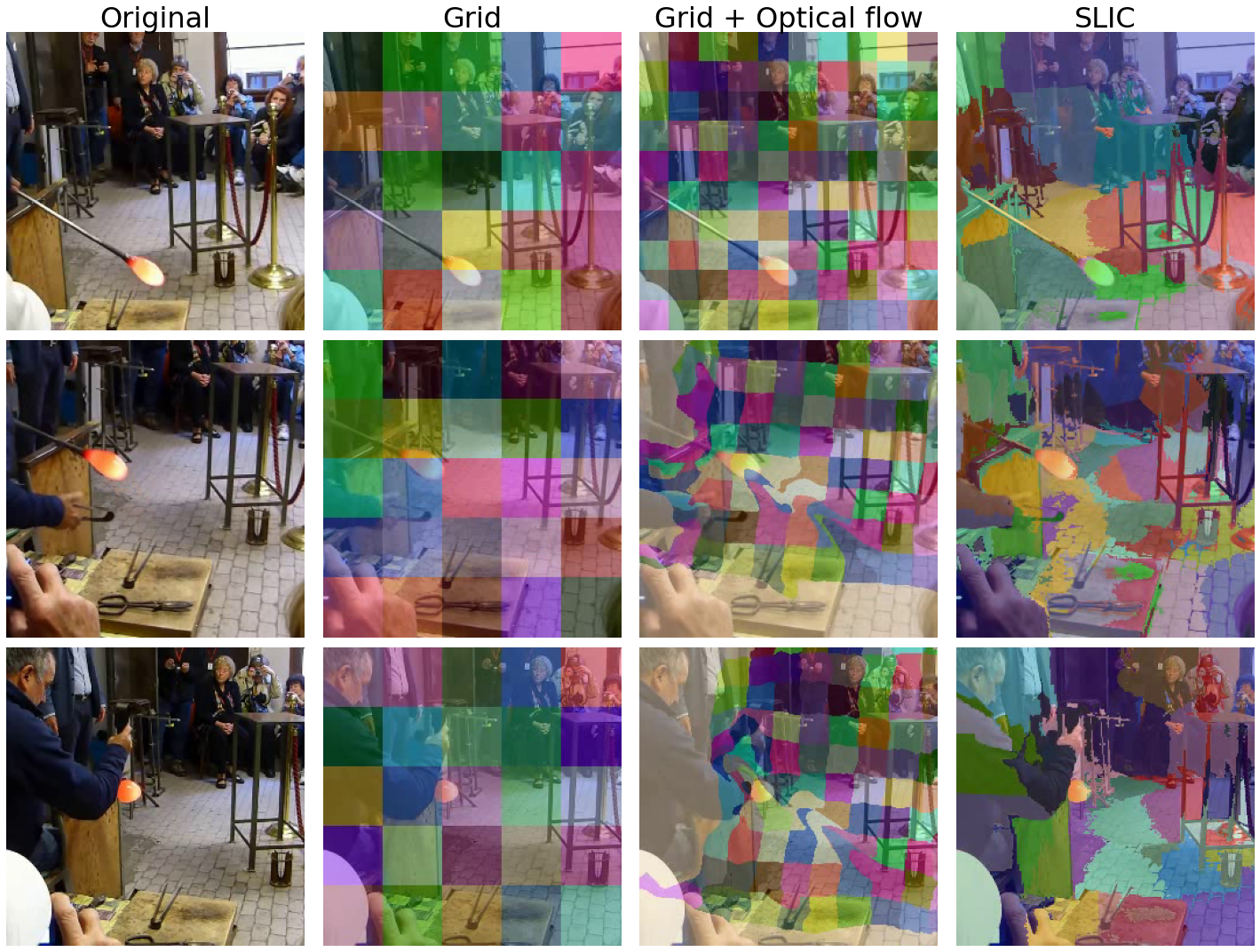
Figure 2: Various video segmentation techniques are displayed in columns, while different frames of the video are depicted in rows. Segmented regions are highlighted in distinct colors over the original video frames. From top to bottom: initial, middle, and final frames of the video. From left to right: unmodified video, basic 3D grid segmentation, 3D grid segmentation with optical flow, and SLIC segmentation. Optical flow estimation was performed using the PWC-Net [28].

One straightforward method for segmenting images or videos involves employing a 2D or 3D grid to establish rectangular or cuboidal patches. While this method boasts simplicity and expedited region generation, it overlooks pixel color information, potentially resulting in similar and proximal pixels being distributed across different regions. This approach is employed in RISE explanations [10] for images and can be extended to videos by adding the temporal dimension to the grid, as depicted in Figure 2.

Alternatively, the adoption of superpixels as features is another option, wherein pixels are grouped based on similarity metrics. Unlike the grid-based approach mentioned earlier, this method is more intricate and time-consuming, yet it gathers comparable pixels into the same regions. For videos, pixels from different frames can be incorporated during superpixel computation. Various superpixel segmentation options for images are demonstrated in Figure 3, encompassing Simple Linear Iterative Clustering (SLIC) [23], which employs K-means in a 5D color space; Quick Shift [29], a kernelized mean-shift approximation; Compact Watershed [30], utilizing marker-driven flooding to define regions with control over compactness; and Felzenswalb’s efficient graph-based image segmentation [31]. The number of segments and their compactness (the balance between spatial and color distance) can be governed by diverse hyperparameters contingent upon the method. Implementation of these techniques can be found in scikit-image’s segmentation package, although only the SLIC segmentation is applicable to video data. Figure 2 illustrates an example of SLIC segmentation applied to video.

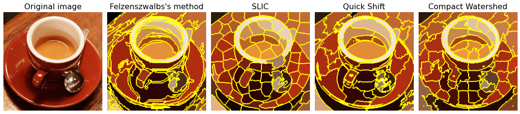
Figure 3: Various image segmentation techniques are illustrated. From left to right: unsegmented image, Felzenszwalb’s method, SLIC, Quick Shift, and Compact Watershed. Segmented regions are outlined in yellow, and the average color was employed to fill each region.

Finally, while many image segmentation methods can be extrapolated to video, an additional approach involves computing optical flow within the video and utilizing it to expand image segmentation from the initial frame to subsequent ones, as demonstrated in [12] for occlusion explanations in videos. However, potential complications arise, particularly when segmenting objects that do not appear in the first frame. This issue is evident in Figure 2, where a substantial region encompassing the individual on the left emerges towards the video’s conclusion, a result of the individual not appearing in the initial frame.

3.2 Feature selection

Feature removal methods operate by observing the impact on the model’s predictions upon removing (or occluding) specific features (or regions). However, certain features may exhibit a more pronounced influence when removed collectively with others, prompting many explanation methods to employ simultaneous removal of multiple features. Given that the number of features removed per sample can influence explanation outcomes, this choice warrants careful consideration during the establishment of the explainability process. Various possibilities for this selection are illustrated in Figure 4.

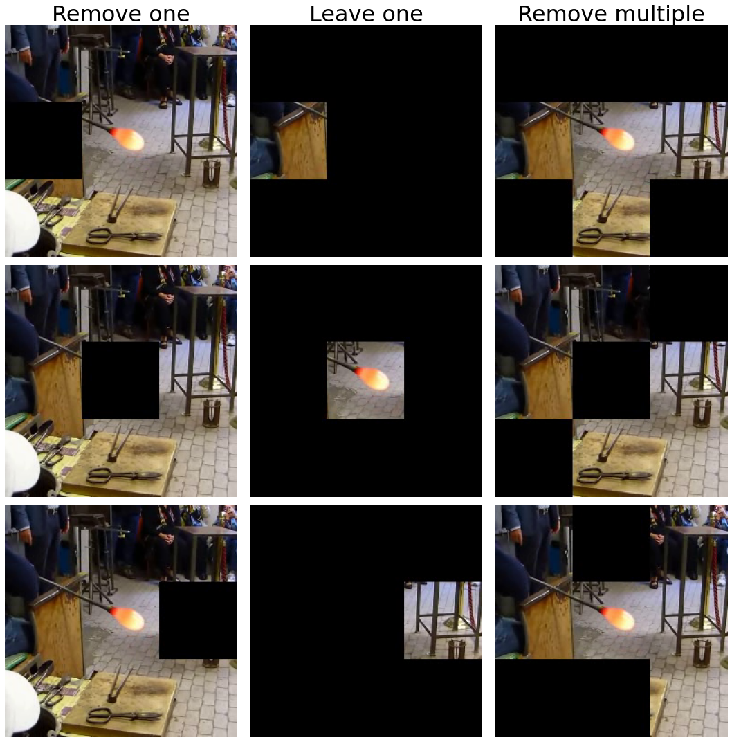
Figure 4: Variations in the feature selection step are depicted. For clarity, individual frames are displayed, although the regions span across subsequent frames. From the leftmost to the rightmost columns: samples with a single occluded feature, samples with only one feature unoccluded, and approximately half of the regions occluded. For the sake of visualization, a 3D grid-based segmentation coupled with black color fill was employed to occlude regions.

One straightforward approach is to remove a single feature for each sample, enabling the assessment of individual feature relevance in model decisions. However, this approach lacks the ability to reveal complex relationships in relevance that become apparent when multiple features are removed simultaneously. Methods employing this form of feature removal include Occlusion Sensitivity [21] and its adaptation to video [12], as well as LOCO [26]. Conversely, an alternative approach involves removing all features except one, as exemplified by the Univariate Predictors method [27].

Alternatively, multiple features can be removed simultaneously, facilitating the identification of significant feature sets. However, this poses a more intricate challenge in uncovering feature relevance. Approaches such as LIME [9], RISE [10], and Kernel SHAP [11] adopt this strategy. In LIME and RISE, each region is either removed or retained with a probability of $p=0.5$, resulting in the occlusion of approximately half the regions. This choice optimizes the minimization of sample requirements for an accurate approximation of feature importance. It is worth noting that altering the probability value to regulate the extent of occluded regions is feasible, and even a hybrid of samples with varying numbers of regions could be employed, although this would likely necessitate an increase in the number of perturbed samples. Kernel SHAP, for instance, follows this strategy by employing a mix of samples with either a few or a greater number of occluded features than those with an approximately uniform amount of occlusions.

3.3 Sample selection

To effectively discern the significance of various features, removal-based methods necessitate perturbed samples of the input to correlate model prediction differences with each feature. Each explanation requires a specific number of model passes, corresponding to the number of samples used, which may vary among explanation methods. Often treated as a hyperparameter, the number of samples can substantially impact the quality of explanation estimates. Striking a balance between estimation accuracy and computational efficiency is vital; it should be sufficiently high to yield insightful explanations while minimized to reduce the computational load.

Certain methods mandate a predetermined number of samples, such as the previously mentioned Occlusion Sensitivity [21], which depends on pixel count and occlusion kernel size, as well as LOCO [26] and Univariate Predictors [27], both reliant on feature count. Conversely, methods like LIME [9], RISE [10], or Kernel SHAP [11] require a user-defined sample count. Generally, increasing the sample count augments the quality of approximated relevance. This is evident in Shapley value estimation using Kernel SHAP, where testing all possible feature combinations is unfeasible; however, a close approximation can be achieved through a substantial sample count, leading to more accurate Shapley value estimates. The appropriate number of samples hinges significantly on the feature count, hence video explanations generally necessitate more samples than image explanations, unless the number of regions is curtailed by enlarging their size. In the RISE publication’s experiment [10], 4,000 or 8,000 samples were used to compute explanations, contingent on the model; the public LIME image implementation defaults to 1,000 samples; and in the Kernel SHAP implementation, the default count is 2,048 plus the number of features.

3.4 Feature removal

In the context of visual data, the concept of removing a pixel does not directly apply; instead, we substitute (or occlude) it with a designated color, effectively nullifying the information it carries. This section delves into various approaches for performing this occlusion, as demonstrated in Figure 5.

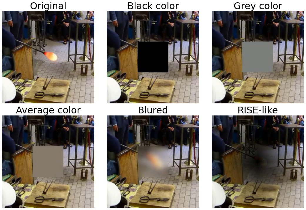
Figure 5: Illustration of feature removal choices adapted from image to video data. Due to space constraints, only single frames are displayed, although the regions span across the entire video duration. The segmentation involves a 3D grid, and for visual clarity, only one region has been occluded in each sample. The sequence depicts, from left to right and top to bottom: unmodified input video, occlusion with a constant black color, occlusion with a constant gray color, occlusion with the average color of the occluded region, occlusion with a uniform blur filter, and RISE-inspired occlusion.

From a color perspective, a straightforward method for occlusion involves filling all regions with a consistent color. Common choices include black (e.g. RISE [10]) or gray (e.g. Occlusion Sensitivity [21]). However, these approaches might suffer from the drawback of generating out-of-domain data by introducing colors not present in the training dataset. To mitigate this concern, a solution is to adopt distinct colors based on the occluded region. For example, the mean color of the occluded region can be used as a replacement, as employed by the image implementation of LIME [9]. Another technique is featured in [32], wherein occlusion is achieved through blurring the region in the image. Alternatively, more sophisticated methods, such as image inpainting [33], could be employed to replace the region in a more intelligent manner. The underlying idea is to eliminate the necessary information for class recognition while preserving the colors present in the image or video. Moreover, it’s possible to retain some level of transparency within the used mask rather than entirely removing the region. This approach is seen in RISE explanations [10], where a low-resolution grid is initially constructed and then scaled up to produce the transparency gradient. This technique allows for smoother occlusion, avoiding the introduction of sharp edges that could result from abrupt occlusion.

3.5 Visualization

The final step in the explainability process is visualization, and although it might appear straightforward, it significantly impacts user comprehension of the explanations. Visualization methods vary based on the explanation technique employed, and this section delves into the decisions to be made in this regard.

An essential divergence among explanation techniques lies in whether computed relevance can solely be positive or whether it can also extend into negative values. Positive relevance is attributed to regions whose removal diminishes confidence in a particular class, indicating their necessity for accurate class prediction. Conversely, negative importance pertains to regions that, when removed, increase confidence in a class, which means that they mislead the model toward incorrect predictions when present. Methods like LIME [9] and SHAP [11] compute both positive and negative relevance, while RISE [10] and Occlusion Sensitivity [21] exclusively produce positive relevance. Visualization of positive relevance often involves a heat map, representing the region’s importance through variations in color intensity. When incorporating both positive and negative relevance, distinct shades of two colors may be used to differentiate them. For instance, LIME uses green and red to denote positive and negative relevance, respectively. An alternative approach involves focusing solely on positive relevance, allowing for the use of heat maps for visualization.

To enhance visualization, histogram stretching can be applied to rescale importance values within the available color space, aiding in the differentiation of relevance across regions. Additionally, rather than displaying all regions, a subset can be chosen, be it the top $n$ significant regions, those surpassing a minimum relevance threshold, or those starting from the most important and incrementally accumulating importance until a set threshold is reached. These methods of reducing displayed regions simplify and refine the explanations by mitigating noise.

Furthermore, explanations can be merged with the input image or video, affording a direct view of the relevance of each pixel for prediction. This can be achieved through alpha compositing, blending explanations with the input data while specifying a transparency value, allowing representation of explanation magnitude. Alternatively, when magnitude is less significant, specific pixel values of the $n$ most important regions can be altered. However, care must be taken to consider the input data’s influence on interpretation, as it can introduce color variations potentially leading to incorrect associations with relevance. For instance, if relevance is displayed in green and the scene already includes green elements, the merge might become ambiguous. This can be addressed by adjusting chosen colors for relevance display or by applying higher transparency to input data and lower transparency to explanations, accentuating explanation colors over the background.

4 Methodology

Following the prescribed framework for conducting local agnostic explanations, as outlined in the previous section, we extend well-established removal-based explainability techniques to accommodate video data. To achieve this, we initially trained three distinct models that form the focal point of our explanations. These models were trained on two datasets characterized by stark dissimilarities. By employing diverse networks and datasets, our intention was to introduce a substantial range in predictions to be explained. This approach allows for a comprehensive evaluation of the explainability techniques across various models, environmental contexts, and classes.

4.1 Networks

We chose three distinct networks to form the foundation of our experiment: TimeSformer [34], TANet [35], and TPN [36]. These selections were motivated by their robust performance in action classification tasks and their user-friendly implementation within MMAction2 [37], an open-source PyTorch-based toolbox designed for video comprehension.

TimeSformer is an adaptation of the Vision Transformer architecture, designed to incorporate spatio-temporal feature learning by leveraging frame-level patches. Among its various iterations, we have chosen the ”divided attention” version, which demonstrated optimal performance. This version excels by independently computing spatial and temporal attention.

TANet encompasses a Temporal Adaptive Module (TAM) embedded within a 2D CNN architecture. This configuration introduces minimal computational overhead while effectively capturing both short and long-term information through a two-level adaptive scheme. The TAM incorporates a local temporal window and a globally derived aggregation weight to achieve this.

TPN, or Temporal Pyramid Network, can be integrated into either 2D or 3D backbones, enhancing model performance—particularly for classes characterized by significant temporal variation. TPN’s methodology involves extracting spatial, temporal, and informational features, which are subsequently rescaled and concatenated.

For both TANet and TPN, we employed the ResNet50 network architecture as the backbone.

4.2 Datasets

We selected two distinct datasets, Kinetics 400 and EtriActivity3D, to assess the explanations on video data. This choice was motivated by the expectation of observing divergent results in both evaluation and explanations, as the datasets exhibit different characteristics.

Kinetics 400 is a sizable dataset containing videos sourced from YouTube, encompassing 400 human action classes, with a minimum of 400 clips per class. These videos center on human interactions, encompassing human-human and human-object scenarios, and exhibit a wide range of individuals, environments, and objects. Moreover, the videos often include camera movements and cuts within the same video, introducing complexities in the data.

On the other hand, EtriActivity3D comprises a smaller set of 55 activity classes, with a total of 112,620 videos. These videos capture daily activities of 100 individuals, with half of the participants being above 64 years old, recorded within their home environments from various rooms and eight perspectives. Apart from the RGB videos, depth frames and skeleton joints data are also available. The videos are recorded using fixed cameras and do not include cuts within a single video, offering a more controlled and stable setting for evaluation.

4.3 Training

For training the three networks (TimeSformer, TANet, and TPN), we utilized a computer equipped with an NVIDIA 4090 GPU and an i9 9900KF CPU, kindly provided by the Universitat de les Illes Balears. We conducted the training and evaluation using MMAction2 [37], an open-source toolbox for video understanding based on PyTorch and part of the OpenMMLab project.

Each model was initialized with pre-trained weights from the Kinetics 400 dataset [38], and further trained for 10 epochs on the EtriActivity3D dataset using K-Cross Validation with K=5. The training of the three models on the Kinetics 400 dataset was deemed unnecessary, as pre-trained weights are readily available and publicly accessible online.

4.4 Explanation Methods

We selected six explanation methods for our experiment: LIME [9], Kernel SHAP [11], RISE [10], LOCO [26], Univariate Predictors [27], and Occlusion Sensitivity [21], all of which have been described in the related work. While LIME, Kernel SHAP, RISE, and Occlusion Sensitivity have already been adapted to image inputs, requiring minimal changes for video input, the remaining two methods, LOCO and Univariate Predictors, needed more substantial modifications to function on video inputs and to provide local explanations instead of global ones. In this section, we detail the adaptations made for each explanation method to work with videos and describe the choices made for each step of the explanation process, summarized in Table 2.

Table 2: Choices by explanation method for the different steps when computing feature removal based video explanations. 3D SOS stands for 3D Sampled Occlusion Sensitivity

	3D LIME	3D Kernel SHAP	3D RISE	LV LOCO	LV Univ. Pred.	3D SOS
Segmentation	SLIC	SLIC	3D grid	SLIC	SLIC	3D grid
(Num. of regions)	$(\approx 200)$	$(\approx 200)$	$(4\cdot 7^{2}=196)$	$(\approx 200)$	$(\approx 200)$	$(1183)$
Feature Selection	Multiple	Multiple	Multiple	All but one	Only one	All but one
Sample Selection	1000	1000	1000	$\approx 200$	$\approx 200$	$(1183)$
Feature Removal	Black	Black	Black	Black	Black	Black
Model behavior	Prediction	Prediction	Prediction	Prediction	Prediction	Prediction
Summary	Linear model	Shapley value	Mean	Difference	Difference	Pred. value
Visualization	Pos./Neg. map	Pos./Neg. map	Heat map	Pos./Neg. map	Pos./Neg. map	Heat map

To adapt LIME and Kernel SHAP to videos, the only step requiring modification was the segmentation process, where pixels of different frames needed to be included in the computation of superpixels. For RISE, we added one dimension to the 2D grid to include temporal information. The LOCO explanations involve multiple trainings of the model, each skipping one feature to perform feature importance attribution. To avoid repeated retraining, we instead computed the difference between occluding or not each feature (or region) independently, which, when compared to the base prediction (with no occlusions), yielded the importance of each feature in a local manner. For LV Univariate Predictors, we changed the method to explain individual predictions (local explanations) rather than the full dataset (global explanations). The importance of a variable (or region) was found by occluding all but that variable and observing the resulting prediction of the model. For Occlusion Sensitivity, we adapted the 2D occlusion kernel to three dimensions and reduced the number of passes through the model by computing only a sample of all possible occlusions. The occlusion process was regulated by introducing a stride value, determining the number of occlusion possibilities in each dimension, which allowed us to manage computational complexity effectively.

For methods using superpixels for video segmentation (LIME, Kernel SHAP, LOCO, and Univariate Predictors), we chose SLIC [23] as the segmentation method due to its ease of extrapolation to three dimensions. We experimentally set the number of segments to approximately 200 and used five times this value as the number of samples for methods requiring this parameter (LIME, Kernel SHAP, and RISE). The occlusion color used for all methods was black.

Figures 6 and 7 present examples of perturbations and explanations, respectively, for each adapted explainability method. The method names have been slightly modified to reflect the changes made: 3D LIME, 3D Kernel SHAP, and 3D RISE (to indicate the extension to three dimensions), LV LOCO, and LV Univariate Predictors (LV standing for Local Visual, as they were modified to serve as local explainers for visual data), and 3D Sampled Occlusion Sensitivity (to highlight the use of sampling with a stride).

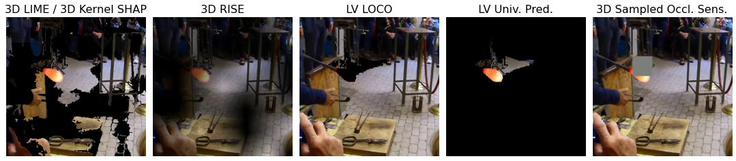
Figure 6: Example of perturbed frame used by each of the explanation methods seen to find the relevance of each region for the correct class. Even though only one frame is shown, perturbations extend to the whole video duration.

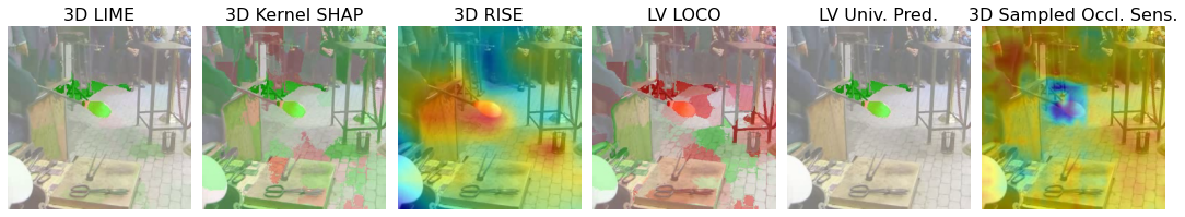
Figure 7: Example of computed explanations on the TimeSformer model and Kinetics 400 dataset, using the different methods. Only one frame of the moment of maximum relevance is shown per method.

4.5 Explanation process

To evaluate the proposed explanation methods, we randomly selected 30 videos from each of the two datasets discussed in subsection 4.2. The selection was not restricted to different classes, allowing for the possibility of having multiple videos from the same class in the sample, while not all classes were necessarily represented. To ensure consistency, we only included videos that were correctly classified by all three networks used in the experiment. Any misclassified videos were replaced with another randomly chosen video.

For each dataset, all 30 videos were passed through each of the three networks described in subsection 4.1, and for each prediction, we generated explanations using each of the video explanation methods detailed in subsection 4.4. This resulted in a total of $30\cdot 2\cdot 3\cdot 6=1080$ explanations.

To improve the visualization of explanations, we retained only the 30% most important regions, thus eliminating noise from less significant regions. Additionally, we applied histogram stretching to utilize the full range of possible colors. Moreover, we removed negative relevance from the explanations for two reasons: to simplify the information presented to users evaluating the explanations and to standardize all the methods, as not all of them provide both positive and negative relevance values.

4.6 Evaluation of the explanations

To comprehensively assess the quality of the generated explanations and enable meaningful comparisons, we adopted two distinct evaluation approaches: automatic evaluations and user-based scoring. Both evaluations were conducted on the same set of 1,080 explanations.

4.6.1 Automatic evaluation

For automatic evaluation, we employed the Insertion and Deletion Game introduced by Fong et al. [32]. We adapted this method in two ways: to ascertain minimal masks and to compute the Area Under the Curve (AUC).

In the context of minimal masks evaluation, the goal is to identify the smallest set of regions that either obstruct sufficient evidence for the network to accurately recognize the correct class (deletion) or provide enough evidence for the correct classification (insertion). To accomplish this, we identified the minimal masks at various target prediction thresholds. The metric value used is the number of pixels present in the masks, expressed as a percentage, as models differ in resolution and frame count.

Inspired by minimal masks evaluation, Petsiuk et al. [10] proposed the AUC as a metric. This method involves computing the area under the curve of the prediction confidence as pixels are deleted or inserted. Unlike the minimal masks evaluation, AUC does not require selecting a specific target prediction threshold but rather summarizes the results across thresholds. AUC should be minimal for deletion (with a minimum value of zero) and maximal for insertion (with a maximum value of one).

In both metrics, we utilized a black color to represent removed regions in the deletion game and as the default value for regions not yet included in the insertion game. This choice ensures consistency with the perturbations used to compute the explanations, which were generated using black color.

4.6.2 User-based evaluation

The user-based evaluation serves the purpose of discerning users’ preferences regarding the types of explanations. It is crucial to emphasize that explanations within AI systems are tailored for human users. Consequently, it becomes imperative to evaluate how these explanations are perceived by humans. To streamline this assessment, a Graphic User Interface (GUI) was developed, as illustrated in Figure 8. The interface displays the video, its associated class, the explanation, and a corresponding color map to aid users in their evaluation.

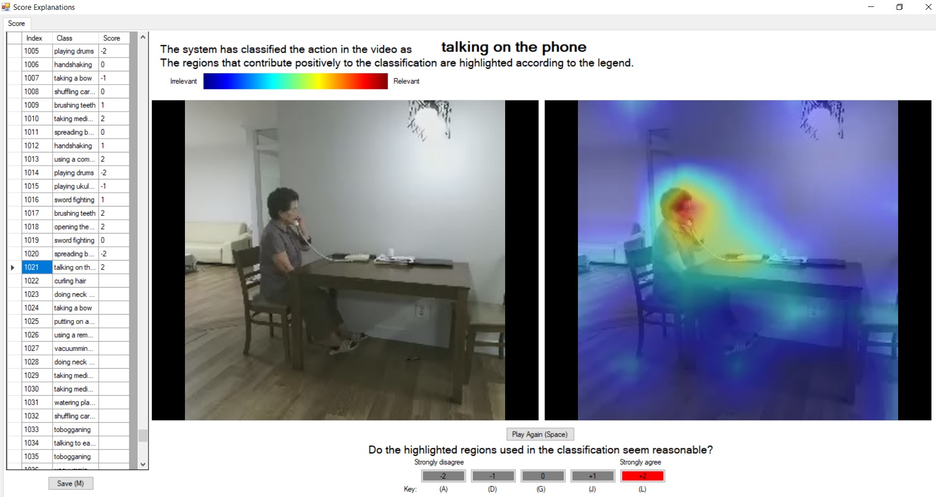
Figure 8: Graphic User Interface (GUI) employed by users to score the explanations. On the left, a list of videos with their corresponding class and the user-assigned scores. At the top, pertinent information about the current explanation is displayed, including the class and the color map representing the explanation. In the center, the video being explained is presented alongside its corresponding explanation. At the bottom, the user is presented with a question, and possible score values are provided, with the selected score shown in red.

The question posed to the users during evaluation is: ”Do the highlighted regions used in the classification seem reasonable?” The available response options range from -2 (strongly disagree) to +2 (strongly agree). This query aims to gauge whether the highlighted regions align with users’ perceptions when identifying specific actions in the video. To mitigate any potential bias, explanations are presented in a random order, and no information regarding the network, dataset, or explanation method is revealed, ensuring a ”blind” evaluation. This evaluation process was conducted by a panel comprising three distinct experts, each applying the same evaluation criteria in the aforementioned way. This evaluation process was conducted by a panel comprising three distinct experts, who scored the same explanations set in the aforementioned way.

5 Results

5.1 Explanation speed

Figure 9 illustrates the average time spent per video for each explanation method, encompassing the segmentation, inference, and explanation stages.

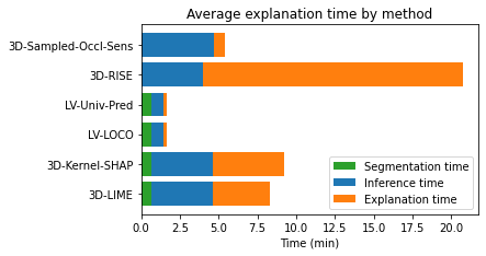
Figure 9: Average time taken by each explanation method to explain a single video, encompassing all three networks and two datasets. The time is broken down into three components: segmentation time, primarily for SLIC computation; inference time, dependent on the network and sample size; and explanation time, primarily allocated to video perturbation.

The segmentation time is noticeable in methods utilizing SLIC to divide the video into regions (all methods except 3D Sampled Occlusion Sensitivity and 3D RISE, which employ grid segmentation), taking approximately 38 seconds.

The inference time, on the other hand, varies depending on the network and scales linearly with the number of samples, which varies across the explanation methods.

The time spent in the computation of explanations, termed ”explanation time”, includes several steps such as perturbation, relevance summary, and visualization. Among these steps, perturbing the videos is the most computationally expensive, influenced by factors such as the type of operations involved and the number of regions occluded per sample. Methods like 3D Sampled Occlusion Sensitivity, LV Univariate Predictors, and LV LOCO exhibit swift video perturbation, as they only occlude one region at a time. In contrast, 3D Kernel SHAP and 3D LIME require more time as they perturb multiple regions simultaneously. The 3D RISE method demands substantially more time compared to other methods due to the use of masks in the range [0, 1] to achieve the fade-in effect.

Regarding the explanation time step, optimizations such as using a faster programming language, algorithmic enhancements, or downsizing the videos being explained can accelerate the process. However, inference time will always depend on the model under explanation.

Figure 10 offers a more detailed breakdown of the time spent on video explanation, categorizing the results by network and dataset.

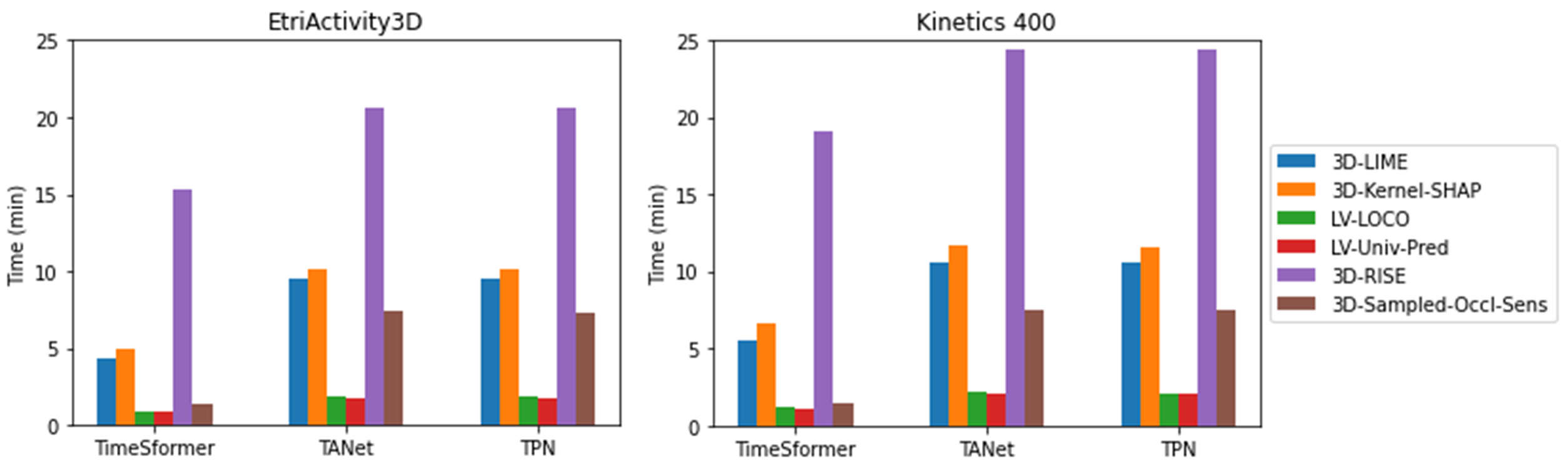
Figure 10: Full list of time taken for the explanation of the predictions of three networks (TimeSformer, TANet and TPN), on videos of two different datasets (EtriActivity3D and Kinetics 400).

5.2 Automatic evaluation

Figure 11 presents the deletion and insertion Area Under the Curve (AUC) values for each explanation method, with results averaged across all networks and datasets. Notable differences in deletion AUC values between datasets are observed. EtriActivity3D exhibits lower deletion AUC values for all explanations across all networks, except for LV Univariate Predictors. Conversely, Kinetics 400 yields better insertion AUC results for all explanations on TimeSformer and TPN. Remarkably, LV Univariate Predictors consistently obtains the poorest results for both deletion and insertion across all datasets and networks.

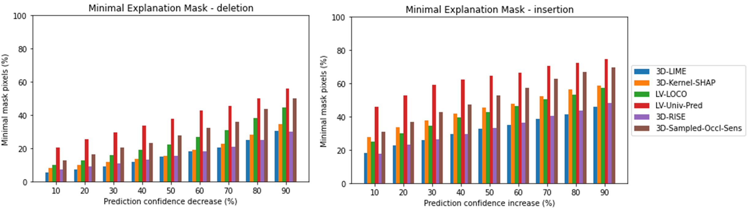
Figure 11: Results of the Minimal Explanation Mask evaluation, averaged across all three networks and two datasets, for each explanation method. On the left, the deletion game results display the minimum percentage of pixels that must be removed from the video to decrease the prediction confidence by different values. On the right, the insertion game results exhibit the minimum percentage of pixels that must be included (to a whole black video) to increase the prediction confidence by different values.

Figure 12 shows the number of pixels in the minimal explanation mask for varying prediction confidence drops or increments, by network and dataset, while Figure 13 shows the average across all networks and datasets. It is evident that 3D LIME, 3D Kernel SHAP, and 3D RISE achieve the best results for both deletion and insertion AUC, with similar values for deletion and 3D LIME slightly outperforming the others in insertion AUC. The choice of the best explanation method, according to this metric, appears to depend on the dataset and network, with the three aforementioned methods consistently performing favorably.

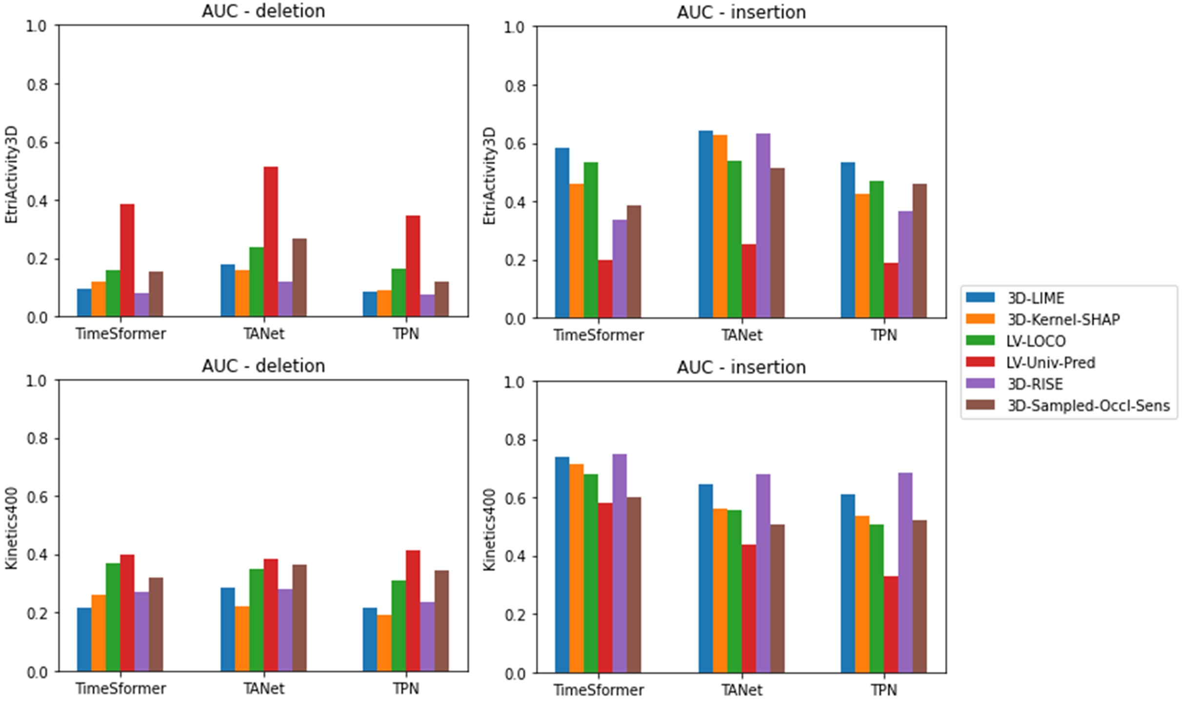
Figure 12: Full list of AUC values for the explanation of the predictions of three networks (TimeSformer, TANet and TPN), on videos of two different datasets (EtriActivity3D and Kinetics 400). In the left column, deletion game; in the right one, insertion game.

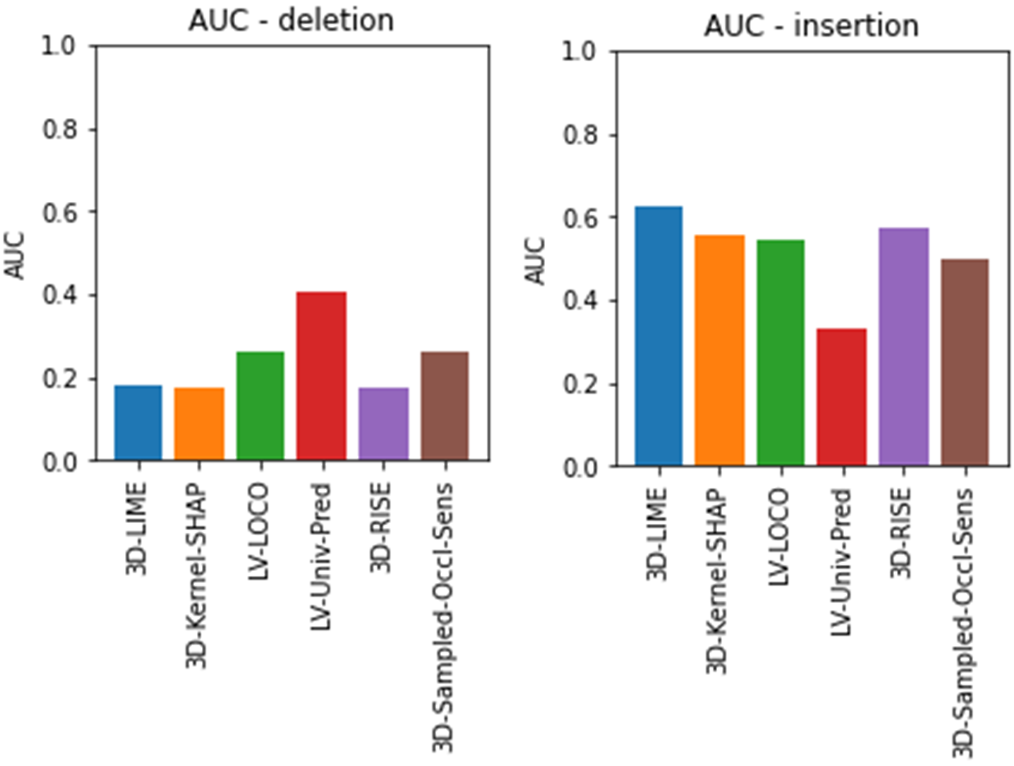
Figure 13: Results of the AUC evaluation metric, averaged across all three networks and two datasets, for each explanation method. At the left, AUC values for the deletion game. At the right, AUC values for the insertion game.

Regarding the Minimal Explanation Mask metric, depicted in Figure 11, it is noteworthy that all methods yield similar results regardless of the prediction confidence choice, displaying a roughly linear increase. For the deletion game, the top three performers are 3D LIME, closely followed by 3D RISE and 3D Kernel SHAP. However, for the insertion game, 3D Kernel SHAP falls behind the other two. LV LOCO, 3D Sampled Occlusion, and LV Univariate Predictors secure the 4th, 5th, and 6th positions, respectively, for both the deletion and the insertion game.

5.3 Evaluation with users

The user-based evaluation results are presented in Figures 14 and 15. Figure 14 illustrates the average scores per method, while Figure 15 aggregates the scores by dataset, network, and method.

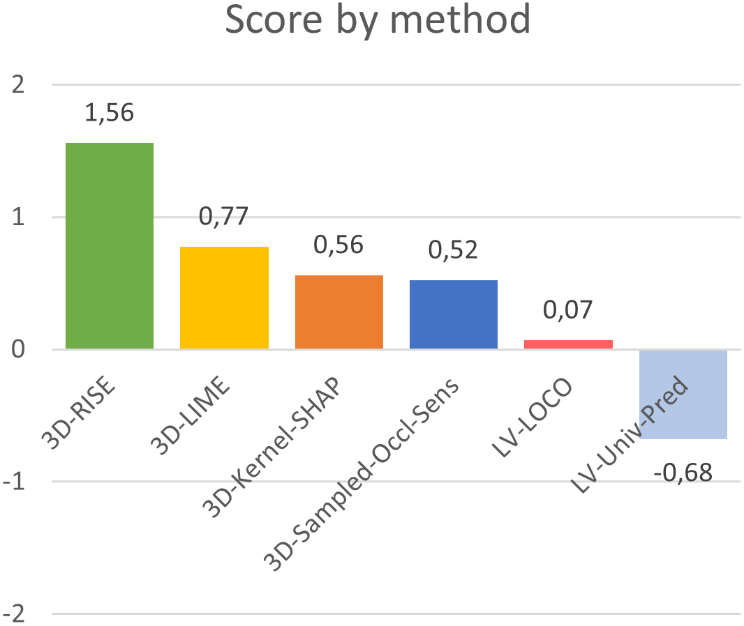
Figure 14: Average scores from the user-based evaluation by explanation methods.

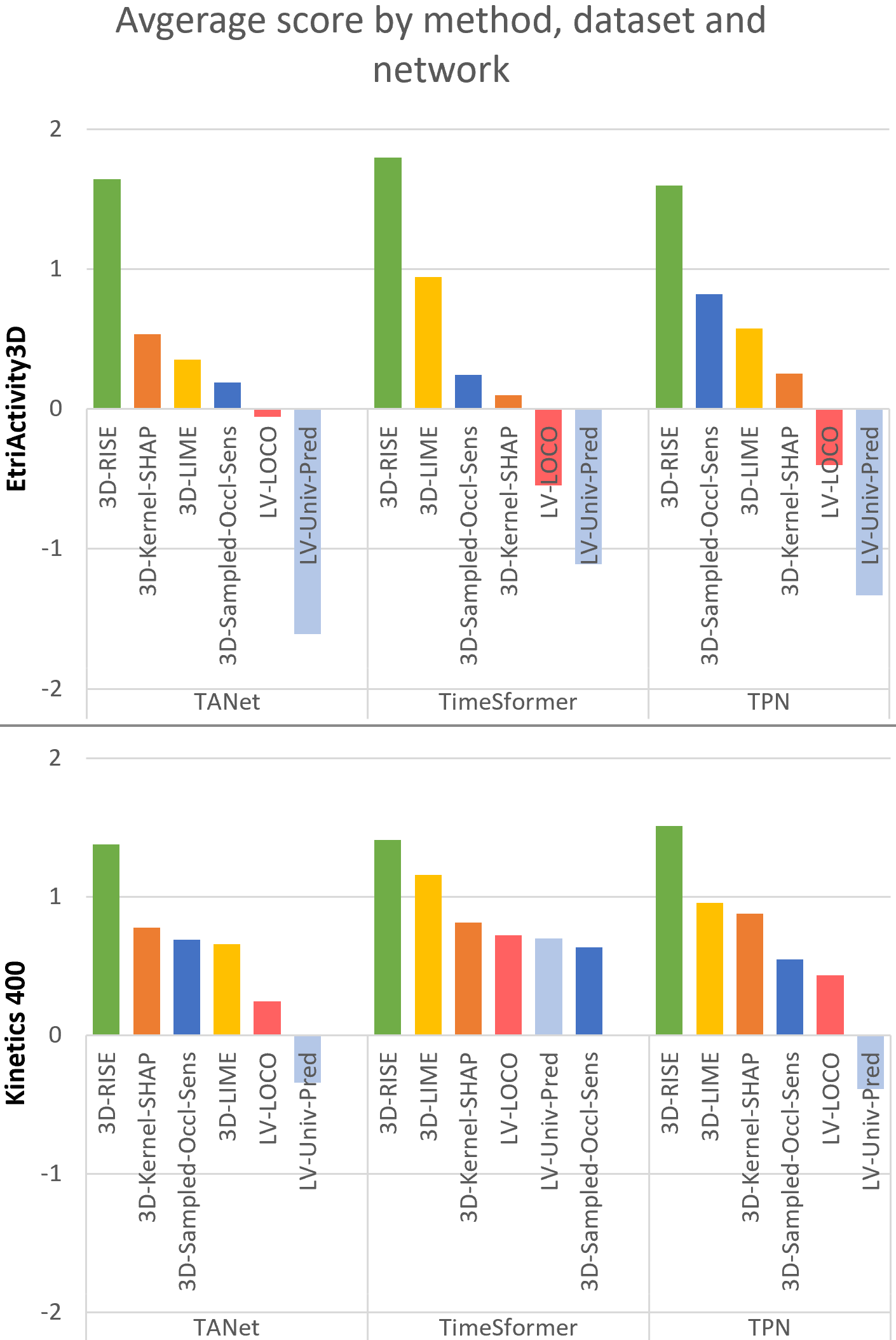
Figure 15: Average scores from the user-based evaluation, grouping by method, dataset and network.

Observing the per-method scores, 3D RISE exhibits the most favorable results, attaining an average score of 1.56 within the range [-2, 2]. In the second position, approximately one point below 3D RISE, is 3D LIME, closely followed by 3D Kernel SHAP and 3D Sampled Occlusion Sensitivity. Conversely, LV LOCO scores poorly, with an average close to zero, and LV Univariate Predictors receives a score of -0.68.

While 3D RISE consistently achieves superior results across datasets and networks, the performance of other methods varies depending on these factors. For instance, LV Univariate Predictors exhibits scores approximately one point higher on Kinetics 400 than on EtriActivity3D, and 3D LIME demonstrates better results on TimeSformer compared to the other two networks. This observation suggests that certain explanation methods may be more suitable for specific network models or particular data characteristics.

On average, the scores on Kinetics 400 are half a point higher than those on EtriActivity3D. However, it is crucial to consider that the Kinetics 400 dataset comprises more challenging videos, featuring camera movements, cuts, and a more extensive range of classes. This discrepancy in scores could be attributed to the inherent difficulty in locating important regions for classification in Kinetics 400 compared to EtriActivity3D. The latter dataset appears to offer a relatively simpler context for region identification, crucial for classification purposes.

6 Discussion

In the context of removal-based explanations for visual data, it is essential to consider various aspects during the explanation process. This study explored individual steps and discussed key parameters such as segmentation methods, occlusion types, and visualization techniques. This analysis aids in classifying existing explanation methods and paves the way for potential improvements by combining strengths from different methods for various steps.

Six distinct explanation methods for video were proposed, all adapted from existing approaches. The adaptation of 3D LIME, 3D Kernel SHAP, and 3D RISE was straightforward, as they were originally designed for images, with the third dimension added solely during the segmentation step. Notably, our adaptation of 3D Sampled Occlusion Sensitivity is more natural and robust to camera movements and cuts compared to the existing adaptation using optical flow [12], enabling relevance discovery in the temporal dimension. Additionally, the novel adaptation of LV LOCO and LV Univariate Predictors to obtain local explanations, instead of global ones, extended their applicability to the vision domain.

To ensure a fair comparison, a comprehensive experiment was designed, enforcing equal conditions for the methods, such as the number of features, samples, occlusion type, and visualization. The selection of hyper-parameters was performed empirically, leaving the investigation of optimal values for future work.

To evaluate the explanation methods, two metrics were chosen from existing literature: the Area Under the Curve (AUC) of the deletion and insertion games, and the Minimal Explanation Mask evaluation. The automated evaluation indicated that 3D RISE and 3D LIME achieved superior explanations for both deletion and insertion variations. Additionally, we conducted a user-based evaluation using a graphical user interface, corroborating the performance of 3D RISE, 3D LIME, and 3D Kernel SHAP. Remarkably, 3D RISE stood out significantly in the user-based evaluation.

The preference for 3D RISE by users suggests that its smooth explanations without hard edges were favored over other methods. This observation prompts the question of whether introducing smoothness, such as through a Gaussian filter, in other methods would positively influence explanation quality according to users. However, it should be noted that this user preference for smoothness did not translate into improved performance in the automated evaluations using AUC and Minimal Explanation Mask.

One drawback of the 3D RISE method is its computational cost, taking more than double the time compared to other methods. This increased computation is due to up-scaling each sample to the size of the video and using masks with a full range between zero and one, rather than binary masks, which slows down the perturbation process. To mitigate this issue, down-sampling the input video frames and perturbing only the frames relevant for the network’s prediction, can significantly improve computational efficiency without compromising the method’s effectiveness.

An important finding was the suboptimal performance of the LV Univariate Predictors method, as evidenced by the user-based evaluation. This may be attributed to excessive perturbations in the explanations, where most samples contain all but one region perturbed. Consequently, these perturbations might lead to samples outside the domain, thereby failing to enhance confidence in the correct class even if the region is crucial for that class. The 3D Kernel SHAP explanations also scored lower compared to 3D LIME, possibly due to the use of many samples with more than half of the regions occluded, leading to potentially misleading or noisy explanations. Further investigation into these aspects is warranted to improve the performance of the LV Univariate Predictors and optimize the 3D Kernel SHAP explanations.

7 Conclusions

In this study, we proposed augmenting Covert et al.’s framework [8] with tailored choices for removal-based explanation methods, specifically aimed at handling visual data. This augmentation is crucial when dealing with video data due to the increased complexity resulting from the temporal dimension. Leveraging this improved framework, we adapted six removal-based explanation methods to the video domain, incorporating necessary adjustments in each case. The evaluation encompassed both automated methods, namely Area Under the Curve (AUC) and Minimal Explanation Mask, for both the deletion and insertion games, along with a user-based evaluation.

The results reveal users’ preference for the 3D RISE method over alternative approaches, attaining average scores of 1.56 within the range [-2, 2]. Both automated and user-based evaluations concur in selecting 3D RISE, 3D LIME, and 3D Kernel SHAP as the superior methods among the six. Despite 3D RISE being computationally expensive, we believe this limitation can be mitigated by reducing the data processing load to only what is necessary for network prediction, i.e. using a limited amount of frames and downsizing them to a determined scale.

Decomposing the explanation process into well-defined steps presents opportunities for investigating the influence of each choice along the explanation pipeline, ultimately enhancing the quality of explanation methods and tailoring them effectively to specific datasets and models. Future research endeavors should explore combining aspects from different methods to derive optimal synergies.

Declarations

Funding Grant PID2019-104829RA-I00 funded by MCIN/AEI/10.13039/ 501100011033, project EXPLainable Artificial INtelligence systems for health and well-beING (EXPLAINING). Grant PID2022-136779OB-C32 funded by MCIN/AEI/ 10.13039/501100011033 and by ERDF A way of making Europe, project Playful Experiences with Interactive Social Agents and Robots (PLEISAR): Social Learning and Intergenerational Communication. F. X. Gaya-Morey was supported by an FPU scholarship from the Ministry of European Funds, University and Culture of the Government of the Balearic Islands.

Conflict of interest The authors have no competing interests to declare that are relevant to the content of this article.

Data availability We do not analyse or generate any datasets, because our work proceeds within a theoretical and mathematical approach.

Appendix A Explanations and AUC curves

Figures 16, 17, and 18 provide illustrative instances of explanations pertaining to the ”taking medicine” class. These examples stem from a sample video extracted from the EtriActivity3D dataset and correspond to explanations generated for the TimeSformer, TANet, and TPN networks, respectively.

Within each figure, the content is organized as follows: arranged vertically in rows are the various explanation methods developed as part of this study. Horizontally, from left to right, the columns represent: the middle frame extracted from the original video, annotated with the respective class label; the explanation presented to users for evaluation purposes; and the deletion and insertion game curves, along with the associated AUC (Area Under the Curve) value. The game curves visually depict the fluctuations in prediction confidence as regions are sequentially added or removed in accordance with their perceived importance.

Figure 16: Explanations and AUC curves for the TimeSformer network.

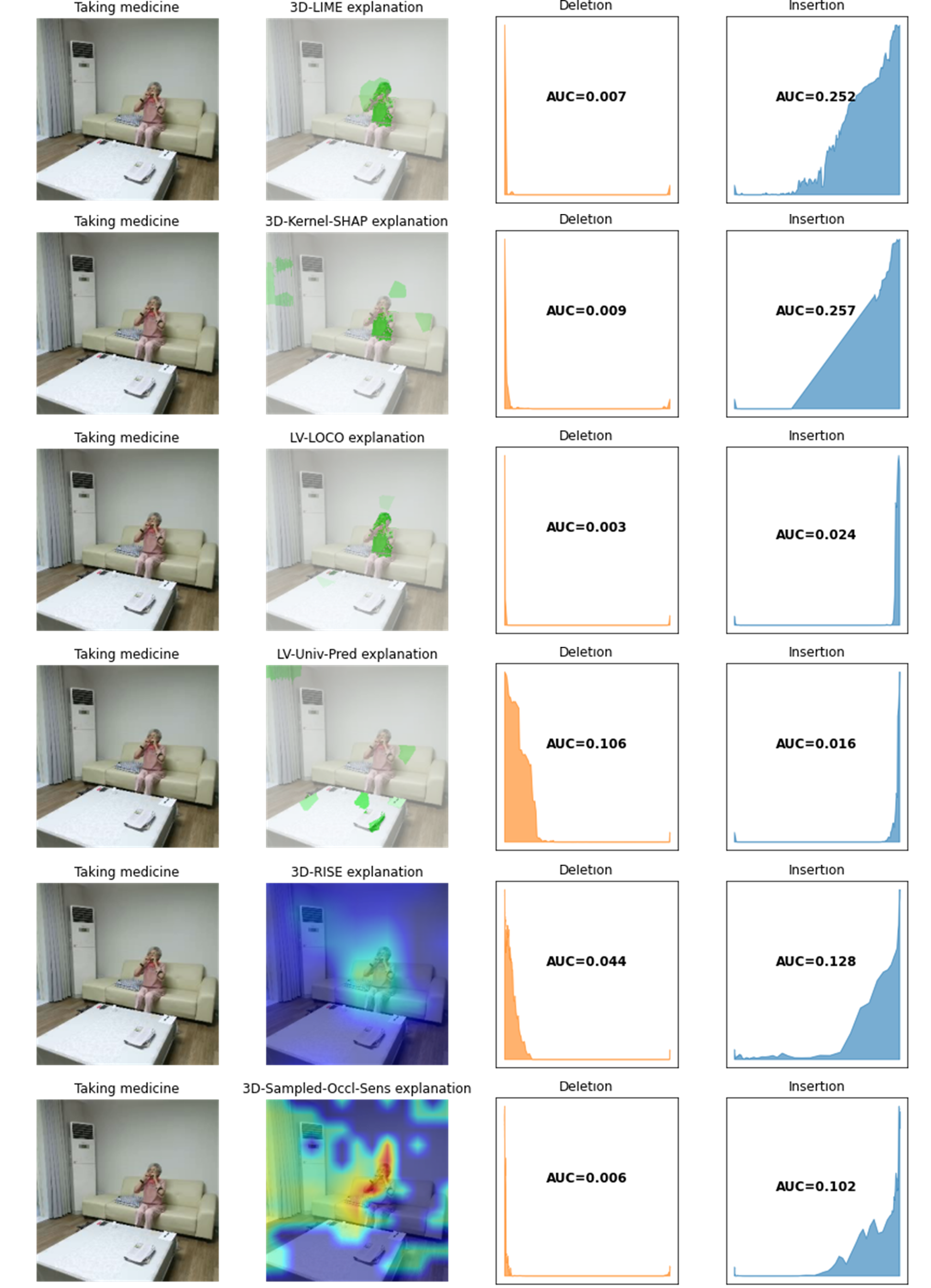
Figure 17: Explanations and AUC curves for the TANet network.

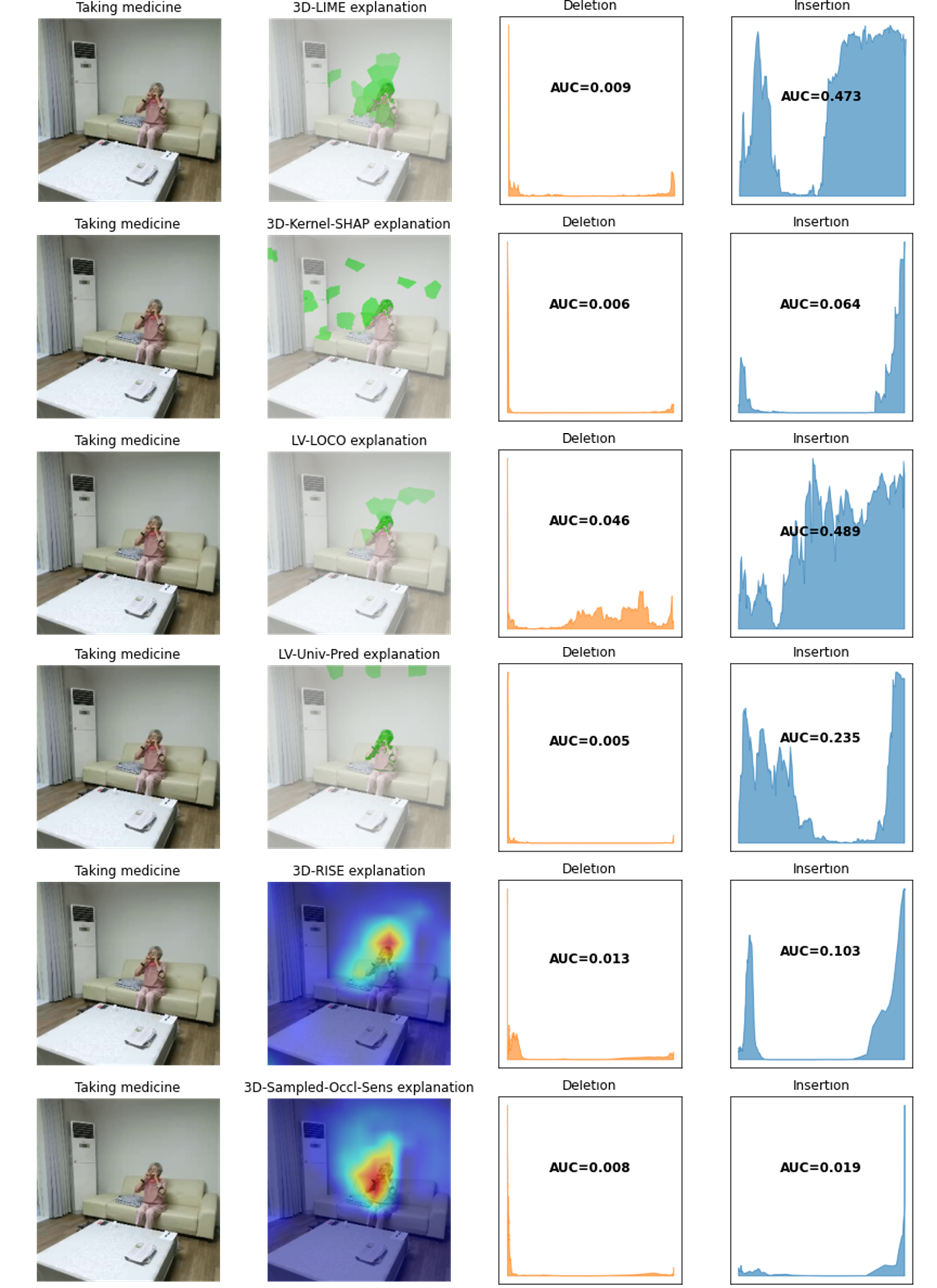
Figure 18: Explanations and AUC curves for the TPN network.

References

- \bibcommenthead
- Barredo Arrieta et al. [2020] Barredo Arrieta, A., Díaz-Rodríguez, N., Del Ser, J., Bennetot, A., Tabik, S., Barbado, A., Garcia, S., Gil-Lopez, S., Molina, D., Benjamins, R., Chatila, R., Herrera, F.: Explainable artificial intelligence (xai): Concepts, taxonomies, opportunities and challenges toward responsible ai. Information Fusion 58, 82–115 (2020)
- Simonyan et al. [2013] Simonyan, K., Vedaldi, A., Zisserman, A.: Deep Inside Convolutional Networks: Visualising Image Classification Models and Saliency Maps. arXiv (2013)
- Bach et al. [2015] Bach, S., Binder, A., Montavon, G., Klauschen, F., Müller, K.-R., Samek, W.: On pixel-wise explanations for non-linear classifier decisions by layer-wise relevance propagation. PLOS ONE 10(7), 1–46 (2015)
- Selvaraju et al. [2017] Selvaraju, R.R., Cogswell, M., Das, A., Vedantam, R., Parikh, D., Batra, D.: Grad-cam: Visual explanations from deep networks via gradient-based localization. In: 2017 IEEE International Conference on Computer Vision (ICCV), pp. 618–626 (2017)
- Hartley et al. [2022] Hartley, T., Sidorov, K., Willis, C., Marshall, D.: Swag-v: Explanations for video using superpixels weighted by average gradients, pp. 1576–1585 (2022)
- Stergiou et al. [2019] Stergiou, A., Kapidis, G., Kalliatakis, G., Chrysoulas, C., Veltkamp, R., Poppe, R.: Saliency tubes: Visual explanations for spatio-temporal convolutions. In: 2019 IEEE International Conference on Image Processing (ICIP), pp. 1830–1834 (2019)
- Hiley et al. [2020] Hiley, L., Preece, A., Hicks, Y., Chakraborty, S., Gurram, P., Tomsett, R.: Explaining Motion Relevance for Activity Recognition in Video Deep Learning Models. arXiv (2020)
- Covert et al. [2021] Covert, I.C., Lundberg, S., Lee, S.-I.: Explaining by removing: A unified framework for model explanation. J. Mach. Learn. Res. 22(1) (2021)
- Ribeiro et al. [2016] Ribeiro, M.T., Singh, S., Guestrin, C.: ”why should i trust you?”: Explaining the predictions of any classifier. In: Proceedings of the 22nd ACM SIGKDD International Conference on Knowledge Discovery and Data Mining. KDD ’16, pp. 1135–1144. Association for Computing Machinery, New York, NY, USA (2016)
- Petsiuk et al. [2018] Petsiuk, V., Das, A., Saenko, K.: RISE: Randomized Input Sampling for Explanation of Black-box Models. arXiv (2018)
- Lundberg and Lee [2017] Lundberg, S.M., Lee, S.-I.: A unified approach to interpreting model predictions. In: Guyon, I., Luxburg, U.V., Bengio, S., Wallach, H., Fergus, R., Vishwanathan, S., Garnett, R. (eds.) Advances in Neural Information Processing Systems, vol. 30. Curran Associates, Inc., ??? (2017)
- Uchiyama et al. [2023] Uchiyama, T., Sogi, N., Niinuma, K., Fukui, K.: Visually explaining 3d-cnn predictions for video classification with an adaptive occlusion sensitivity analysis. In: 2023 IEEE/CVF Winter Conference on Applications of Computer Vision (WACV), pp. 1513–1522 (2023)
- Li et al. [2021] Li, Z., Wang, W., Li, Z., Huang, Y., Sato, Y.: Towards visually explaining video understanding networks with perturbation. In: 2021 IEEE Winter Conference on Applications of Computer Vision (WACV), pp. 1119–1128 (2021)
- Stergiou et al. [2019] Stergiou, A., Kapidis, G., Kalliatakis, G., Chrysoulas, C., Poppe, R., Veltkamp, R.: Class feature pyramids for video explanation. In: 2019 IEEE/CVF International Conference on Computer Vision Workshop (ICCVW), pp. 4255–4264 (2019)
- Hiley et al. [2019] Hiley, L., Preece, A., Hicks, Y., Marshall, D., Taylor, H.: Discriminating Spatial and Temporal Relevance in Deep Taylor Decompositions for Explainable Activity Recognition. arXiv (2019)
- Bargal et al. [2018] Bargal, S.A., Zunino, A., Kim, D., Zhang, J., Murino, V., Sclaroff, S.: Excitation backprop for rnns. In: 2018 IEEE/CVF Conference on Computer Vision and Pattern Recognition, pp. 1440–1449 (2018)
- Anders et al. [2018] Anders, C., Montavon, G., Samek, W., Müller, K.-R.: Understanding Patch-Based Learning by Explaining Predictions. arXiv (2018)
- Montavon et al. [2017] Montavon, G., Lapuschkin, S., Binder, A., Samek, W., Müller, K.-R.: Explaining nonlinear classification decisions with deep taylor decomposition. Pattern Recognition 65, 211–222 (2017)
- Srinivasan et al. [2017] Srinivasan, V., Lapuschkin, S., Hellge, C., Müller, K.-R., Samek, W.: Interpretable human action recognition in compressed domain. In: 2017 IEEE International Conference on Acoustics, Speech and Signal Processing (ICASSP), pp. 1692–1696 (2017)
- Gan et al. [2015] Gan, C., Wang, N., Yang, Y., Yeung, D.-Y., Hauptmann, A.G.: Devnet: A deep event network for multimedia event detection and evidence recounting. In: 2015 IEEE Conference on Computer Vision and Pattern Recognition (CVPR), pp. 2568–2577 (2015)
- Zeiler and Fergus [2014] Zeiler, M.D., Fergus, R.: Visualizing and understanding convolutional networks. In: Fleet, D., Pajdla, T., Schiele, B., Tuytelaars, T. (eds.) Computer Vision – ECCV 2014, pp. 818–833. Springer, Cham (2014)
- Hartley et al. [2021] Hartley, T., Sidorov, K., Willis, C., Marshall, D.: Swag: Superpixels weighted by average gradients for explanations of cnns. In: Proceedings of the IEEE/CVF Winter Conference on Applications of Computer Vision (WACV), pp. 423–432 (2021)
- Achanta et al. [2010] Achanta, R., Shaji, A., Smith, K., Lucchi, A., Fua, P., Süsstrunk, S.: Slic superpixels, 15 (2010)
- Springenberg et al. [2014] Springenberg, J.T., Dosovitskiy, A., Brox, T., Riedmiller, M.: Striving for Simplicity: The All Convolutional Net. arXiv (2014)
- Fong et al. [2019] Fong, R., Patrick, M., Vedaldi, A.: Understanding deep networks via extremal perturbations and smooth masks. In: 2019 IEEE/CVF International Conference on Computer Vision (ICCV), pp. 2950–2958 (2019)
- Lei et al. [2018] Lei, J., G’Sell, M., Rinaldo, A., Tibshirani, R.J., Wasserman, L.: Distribution-free predictive inference for regression. Journal of the American Statistical Association 113(523), 1094–1111 (2018)
- Guyon and Elisseeff [2003] Guyon, I., Elisseeff, A.: An introduction to variable and feature selection. Journal of machine learning research 3(Mar), 1157–1182 (2003)
- Sun et al. [2018] Sun, D., Yang, X., Liu, M.-Y., Kautz, J.: Pwc-net: Cnns for optical flow using pyramid, warping, and cost volume. In: Proceedings of the IEEE Conference on Computer Vision and Pattern Recognition, pp. 8934–8943 (2018)
- Vedaldi and Soatto [2008] Vedaldi, A., Soatto, S.: Quick shift and kernel methods for mode seeking. In: Forsyth, D., Torr, P., Zisserman, A. (eds.) Computer Vision – ECCV 2008, pp. 705–718. Springer, Berlin, Heidelberg (2008)
- Neubert and Protzel [2014] Neubert, P., Protzel, P.: Compact watershed and preemptive slic: On improving trade-offs of superpixel segmentation algorithms. In: 2014 22nd International Conference on Pattern Recognition, pp. 996–1001 (2014)
- Felzenszwalb and Huttenlocher [2004] Felzenszwalb, P.F., Huttenlocher, D.P.: Efficient graph-based image segmentation. International Journal of Computer Vision 59(2), 167–181 (2004)
- Fong and Vedaldi [2017] Fong, R.C., Vedaldi, A.: Interpretable explanations of black boxes by meaningful perturbation. In: Proceedings of the IEEE International Conference on Computer Vision (ICCV) (2017)
- Xie et al. [2012] Xie, J., Xu, L., Chen, E.: Image denoising and inpainting with deep neural networks. In: Pereira, F., Burges, C.J., Bottou, L., Weinberger, K.Q. (eds.) Advances in Neural Information Processing Systems, vol. 25. Curran Associates, Inc., ??? (2012)
- Bertasius et al. [2021] Bertasius, G., Wang, H., Torresani, L.: Is Space-Time Attention All You Need for Video Understanding? arXiv (2021)
- Liu et al. [2020] Liu, Z., Wang, L., Wu, W., Qian, C., Lu, T.: Tam: Temporal adaptive module for video recognition. arXiv preprint arXiv:2005.06803 (2020)
- Yang et al. [2020] Yang, C., Xu, Y., Shi, J., Dai, B., Zhou, B.: Temporal pyramid network for action recognition. In: Proceedings of the IEEE Conference on Computer Vision and Pattern Recognition (CVPR) (2020)
- Contributors [2020] Contributors, M.: OpenMMLab’s Next Generation Video Understanding Toolbox and Benchmark. https://github.com/open-mmlab/mmaction2 (2020)
- Kay et al. [2017] Kay, W., Carreira, J., Simonyan, K., Zhang, B., Hillier, C., Vijayanarasimhan, S., Viola, F., Green, T., Back, T., Natsev, P., Suleyman, M., Zisserman, A.: The Kinetics Human Action Video Dataset. arXiv (2017)