Knowledge Distillation on Spatial-Temporal Graph Convolutional Network for Traffic Prediction

Abstract

Efficient real-time traffic prediction is crucial for reducing transportation time. To predict traffic conditions, we employ a spatio-temporal graph neural network (ST-GNN) to model our real-time traffic data as temporal graphs. Despite its capabilities, it often encounters challenges in delivering efficient real-time predictions for real-world traffic data. Recognizing the significance of timely prediction due to the dynamic nature of real-time data, we employ knowledge distillation (KD) as a solution to enhance the execution time of ST-GNNs for traffic prediction. In this paper, We introduce a cost function designed to train a network with fewer parameters (the student) using distilled data from a complex network (the teacher) while maintaining its accuracy close to that of the teacher. We use knowledge distillation, incorporating spatial-temporal correlations from the teacher network to enable the student to learn the complex patterns perceived by the teacher. However, a challenge arises in determining the student network architecture rather than considering it inadvertently. To address this challenge, we propose an algorithm that utilizes the cost function to calculate pruning scores, addressing small network architecture search issues, and jointly fine-tunes the network resulting from each pruning stage using KD. Ultimately, we evaluate our proposed ideas on two real-world datasets, PeMSD7 and PeMSD8. The results indicate that our method can maintain the student’s accuracy close to that of the teacher, even with the retention of only $3\%$ of network parameters.

1 Introduction

Traffic prediction has gained significant importance due to the increasing use of vehicles in various contexts such as transportation of goods, city taxis, personal cars, buses, etc. [1, 2]. The data used for traffic prediction is obtained by monitoring stations in various urban areas. These stations record various parameters, including vehicle speed, traffic density, traffic flow, and …, at specific time periods. These records can be modeled as temporal graphs through preprocessing [1]. Each graph node represents the traffic data of each monitoring station and connections between these stations indicate graph edges. With this data in hand, spatio-temporal graph neural networks will be capable of predicting future traffic conditions for each of the graph nodes at desired time intervals. In real-world traffic prediction, dealing with a large number of nodes can be computationally expensive and may demand substantial hardware resources. Our objective is to propose an idea to enhance the execution time of spatio-temporal graph convolutional networks (ST-GCNs) within the domain of traffic prediction. These networks serve as robust tools in deep learning and complex data analysis, dedicated to predicting relationships among various elements within spatio-temporal systems.
Leveraging knowledge distillation [4], we formulate a network that, owing to its reduced number of parameters and subsequently lower execution time, can accurately predict traffic comparable to that of a complex network. Initially, through knowledge distillation, we introduce a cost function that trains a network with fewer parameters, denoted as the ”student,” by drawing insights from a comprehensive model known as the ”teacher.” This training occurs under the consideration of spatial-temporal structures and their temporal relationships in graphs. The objective is to equip the student network with accuracy akin to the teacher model. While knowledge distillation effectively addresses the challenge of training a compact network, it falls short in providing guidance on the architecture of the student network. To overcome this, we introduce a pruning algorithm capable of identifying and eliminating insignificant parameters in a complex teacher network. In leveraging knowledge distillation, we view parameter learnability as a solution for elimination. The algorithm adeptly prunes the network while jointly training it using knowledge distillation.
We evaluate our proposed cost function and algorithm using two real-world traffic datasets: PeMSD7, comprising 228 nodes, and PeMSD8, consisting of 170 nodes. The results demonstrate that the student trained with our cost function outperforms previous approaches in terms of knowledge distillation and execution time. Additionally, we showcase that our pruning algorithm effectively determines the architecture of the student network, enhancing learnability during training with knowledge distillation compared to when the algorithm does not employ knowledge distillation.
In the following subsection, we will provide further explanation of the proposed knowledge distillation and pruning algorithm.

1.1 Knowledge Distillation and Pruning

Knowledge distillation (KD) and Pruning are two complementary techniques employed in this study for model compression and performance enhancement. KD, serving as a model compression approach, involves transferring knowledge from a complex teacher model to a simpler student model, with the aim of reducing computational overhead [4, 8, 9, 10]. This process entails training the smaller network in an optimized manner to mitigate potential accuracy loss resulting from parameter reduction [4].
In the specific context of ST-GNNs for traffic prediction, KD offers advantages such as reducing model size and the number of parameters, with the teacher model transferring spatial and temporal complexities to the student model for accelerated learning while maintaining accuracy.
Knowledge distillation (KD) is categorized into response-based, feature-based, and relation-based methods [11, 12, 13, 14, 15, 16, 17]. Response distillation focuses on the final layer’s output, while feature distillation targets intermediate layers. This paper adopts both response-based and feature-based knowledge distillation methods. Additionally, KD can be classified based on distillation strategy into offline, online, and self-distillation [18, 19, 20]. The chosen strategy in this work is offline distillation, where both student and teacher networks are updated. An inherent challenge in KD is the selection of the student network structure, addressed in this study by intentionally reducing parameters in the student network compared to the teacher model. The paper utilizes pruning methods to achieve this reduction, and the remaining student network parameters’ learnability is a key criterion for employing KD.
Pruning, as a separate neural network compression technique, is employed to reduce model complexity and enhance performance by eliminating unnecessary parameters and connections [5, 21].
Specifically, in this study, pruning is applied to filters in hidden layers, involving the removal of weights or connections with the lowest importance based on specified thresholds derived from methods like gradient analysis or entropy information [6]. The integration of KD into the pruning process establishes criteria for assessing the impact of network parameters on model accuracy and their ability to learn from the distilled data provided by the teacher model. The evaluation of parameter competency becomes a crucial criterion in the joint application of knowledge distillation and pruning.
The structure of the paper is organized as follows: Section 2 explores related works on knowledge distillation, network pruning, and spatio-temporal graph neural networks. Section 3 introduces a ST-GNN model and the proposed knowledge distillation methods. It also discusses a pruning algorithm designed to address challenges in the student network architecture. Section 4 evaluates the performance of various cost functions on the PeMSD7 and PeMSD8 datasets, presenting ablation studies and analyzing their results. Finally, Section 5 outlines future works and draws conclusions.

2 Related Works

2.1 Traffic Prediction and Spatio-Temporal Graph Neural Networks

Fast and accurate traffic prediction is essential for urban traffic control and management, particularly for medium and long-term forecasts. Traditional methods often struggle with these predictions due to the complexities of traffic flows and the neglect of spatial and temporal dependencies. To address this, deep networks capable of handling temporal and spatial data have been proposed. In [22], the paper discusses the significance of traffic network prediction and its applications, such as network monitoring, resource management, and threat detection. Various recurrent neural network architectures, including standard RNN, LSTM, and GRU, are explored for network traffic prediction. In [23], the development and evaluation of short-term traffic prediction models using bidirectional and unidirectional long short-term memory (LSTM) neural networks are examined. Bidirectional LSTM (BiLSTM) models outperform unidirectional LSTM (Uni-LSTM) models, especially for speed and traffic flow prediction.
A combination of uni-LSTM and BiLSTM architectures also enhances 15-minute predictions. However, LSTM and RNN networks have high execution times due to numerous parameters. For low-latency traffic prediction, spatio-temporal graph neural networks are introduced. These networks utilize graph convolution layers for spatial processing and convolution layers for capturing temporal correlations, offering reduced execution time and comparable or better accuracy.
In [3], the spatio-temporal graph convolutional network (ASTGCN) model is introduced to predict traffic flow. ASTGCN addresses challenges in modeling spatial-temporal correlations in traffic data, using three components to capture recent, daily, and weekly dependencies. Spatial-temporal attention mechanisms and convolution layers effectively capture traffic data patterns, outperforming other methods in traffic flow prediction. In  [1], the spatio-temporal graph convolutional networks (STGCN) framework is presented for time series prediction in traffic management. STGCN employs a graph-based convolutional structure, which enhances training efficiency and captures comprehensive spatial-temporal correlations. It consists of two spatio-temporal convolution blocks and a fully connected layer for making predictions. This approach outperforms other methods on real traffic datasets, providing a more efficient solution for traffic forecasting.

2.2 Knowledge Distillation

Knowledge Distillation, also known as Teacher-Student Learning, is a method introduced in the paper [4] in 2015. In [4], the authors introduced knowledge distillation, a method that transfers knowledge from a complex and accurate neural network (the ”teacher”) to a smaller and more efficient neural network (the ”student”). The aim is to align the behavior and predictions of the student network with the teacher network, allowing the student to benefit from the rich knowledge of the teacher, leading to improved performance and reduced computational resources required for predictions. Initially, knowledge distillation was applied to training smaller models from complex ones, with the teacher network being a complex, accurate neural network with many parameters, and the student network being trained to align its outputs with the teacher’s, resulting in improved performance and efficiency. In further research, knowledge distillation extended to graph networks and spatiotemporal graph networks.
In [25], the focus is on knowledge transfer in Convolutional Neural Networks (CNN) and graph convolutional networks (GCN), introducing a novel approach for knowledge transfer from a GCN teacher model to a GCN student model, leading to a smaller model with improved execution time, particularly suited for dynamic graph models. In [26], the objective is to train a simpler network through knowledge distillation from multiple GCN teacher models with different tasks, extending to distill spatial graph information from hidden convolutional layers. This approach empowers the student model to excel in various tasks without additional labeled data. In [27], knowledge distillation is extended to spatio-temporal graph neural networks for modeling spatial and temporal data in human body position videos, utilizing various techniques, including minimizing loss, leveraging spatial-temporal relations, and using the gradient rejuvenation method to optimize the student model with distilled knowledge from the teacher.

2.3 Pruning and Fine-Tuning

In 1990, the concept of neural network pruning was first presented in the paper by [5]. Pruning involves eliminating unnecessary connections or neurons from trained neural networks to enhance computational efficiency without compromising network performance significantly. The authors presented a method for identifying connections safe to prune using the Hessian matrix associated with the network’s error function. This approach aims to reduce the parameters in large neural networks, lowering the risk of overfitting, decreasing computational resource requirements, and facilitating deployment on resource-constrained devices. Pruning connections has become an essential tool for compressing neural networks and optimizing models for efficient deployment across various applications.
In 2019, [6] introduced a method for estimating the importance of layers and weights in neural networks, enabling the removal of unimportant weights and reducing network size. This method accurately assesses the importance of each layer and network parameter, followed by the removal of unimportant weights. The iterative pruning and retraining stages enhance performance and reduce model complexity. Removing unimportant weights reduces network size, leading to reduced computational resource consumption and improved model execution speed. This approach offers a substantial improvement in compressing large network models.

3 Proposed Methods

Traffic prediction, involves predicting future values of key traffic conditions (e.g., speed or traffic flow) for the next $h$ time steps based on $M$ prior traffic observations. The observation vector $V_{t}\in\mathbb{R}^{N}$ at time step $t$ consists of data from $N$ monitoring stations, encompassing information like speed and traffic flow. Each time step generates a new observation vector. In this paper, we model the traffic network as graphs defined across time steps. The $N$ components of observation $V_{t}$ are interconnected through pairwise connections in the graph, making the data points $V_{t}$ graph signals in a directed graph $G$ with weights $W_{ij}$. At time step $t$, data from $N$ monitoring stations is represented as a graph $G_{t}=(V_{t},E,W)$, where $V_{t}$ contains features from $N$ nodes (e.g., road segments) with speed as the chosen criterion. The edge set $E$ depicts connections between stations, defined based on distance criteria, reflecting the influence of stations on each other. Weights $W\in\mathbb{R}^{N\times N}$ in the weighted adjacency matrix signify the relationships between stations, often determined by spatial disparities.

Table 1: Network information for knowledge distillation and pruning

   PeMSD7 Models Parameters Hidden Blocks Channel Test Time (s) FLOPS Teacher 333,604 [1, 32, 64][64, 32, 128] 3.423 49,889,172,087 Pruning Base Model 48,628 [1, 8, 16][16, 8, 32] 1.069 9,113,934,711 Student 10,144 [1, 2, 4][4, 2, 8] 0.547 1,726,990,455

   PeMSD7 Models Parameters Hidden Blocks Channel Test Time (s) FLOPS Teacher 296,426 [1, 32, 64][64, 32, 128] 2.556 40,636,466,453 Pruning Base Model 39,290 [1, 8, 16][16, 8, 32] 0.810 5,659,617,749 Student 7,766 [1, 2, 4][4, 2, 8] 0.441 1,003,700,933

3.1 Neural Architecture

The ST-GCN[1], designed for traffic prediction, processes spatial and temporal data. Graph convolution layers capture spatial relationships and node features over time. Convolutional layers model temporal correlations, focusing on sequential patterns and changes between graphs. The architecture comprises two blocks with temporal and spatial layers, and an output block transforms information into the final output. The teacher and student networks share an identical number of blocks and layers. Any variations in parameters result from differences in channel numbers within the temporal and spatial layers of the hidden layer. The complex ST-GCN teacher network achieves high accuracy with 333,604 and 296,426 parameters for PeMSD7 and PeMSD8 datasets ( Table 1 and Figure 1 ). Despite accuracy, its high parameter count results in significant computational cost. The challenge lies in balancing accuracy and computational cost, crucial for selecting models. To address the need for a lighter model, the student network is a scaled-down version of the teacher network. With 10,144 and 7,766 parameters for PeMSD7 and PeMSD8 ( Table 1 and Figure 1 ), it maintains accuracy while reducing complexity and computational requirements. This lightweight solution is efficient for traffic prediction, especially in resource-constrained scenarios.

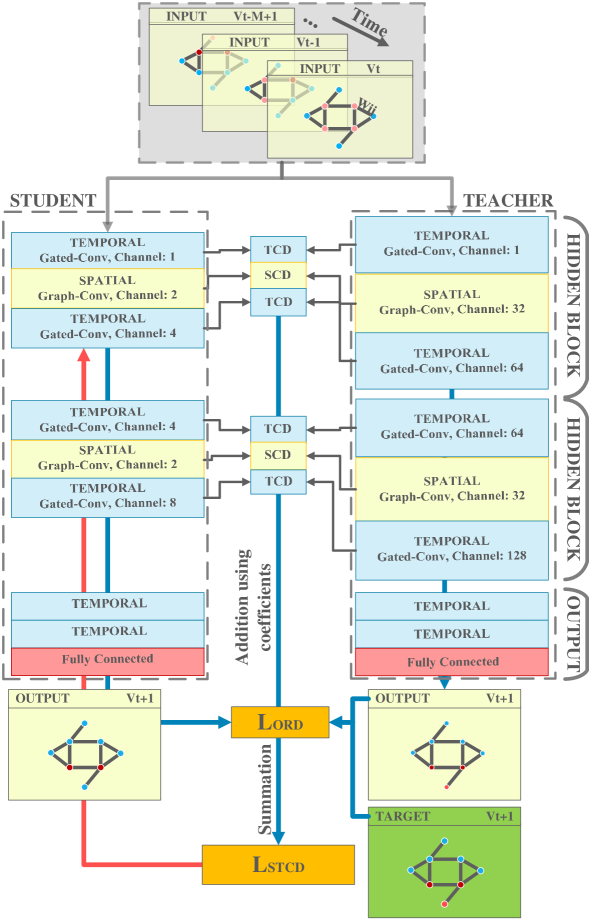
Figure 1: The illustration features both our student and teacher models, demonstrating the application of our cost functions to the spatio-temporal graph convolutional network (ST-GCN)

3.2 Knowledge Distillation

We utilized two knowledge distillation techniques. The initial approach, known as response-based distillation, involves transmitting crucial information from the teacher network’s outputs to the student network. This leads to the development of a simpler and faster model while simultaneously preserving performance. The second method, feature-based knowledge distillation, focuses on hidden layers’ knowledge, encompassing spatial and temporal correlations among graph nodes (Figure 1). Knowledge distillation proves valuable for transferring knowledge from complex networks to simpler ones, particularly in resource-constrained environments requiring rapid algorithm execution.

3.2.1 Response-based Distillation

Leveraging the L2 and Kullback-Leibler (KL) divergence metrics, these functions measure the differences between the teacher and student network outputs [27, 28, 30, 29, 25]. The student network endeavors to enhance its accuracy compared to the teacher by minimizing these error functions. Equations (2) and (3) employ the L2 error function to quantify the difference between the outputs of the teacher and student networks for each node. This function assesses accuracy by summing the squared differences between the values of each network. The KL divergence error function in Equation 3 gauges the disparity between the probability distributions of the outputs of the teacher and student networks.

$$\forall b\in B,\forall i\in N:\quad\text{KL}(y^{s}_{bi},y^{t}_{bi})=y^{t}_{bi}\log\left(\frac{y^{t}_{bi}}{y^{s}_{bi}}\right)$$ (1)

$$\forall b\in B,\forall i\in N:\quad L_{\mathrm{RD(KL)bi}}=\beta\cdot\text{KL}(y^{s}_{bi},y^{t}_{bi})+(1-\beta)\cdot\|y^{s}_{bi}-T_{bi}\|_{2}$$ (2)

$$\forall b\in B,\forall i\in N:\quad L_{\mathrm{RD(L2)bi}}=\beta\cdot\|y^{s}_{bi}-y^{t}_{bi}\|_{2}+(1-\beta)\cdot\|y^{s}_{bi}-T_{bi}\|_{2}$$ (3)

In these equations, $||\cdot||_{2}$ denotes the L2 norm. The variables $N$, $y^{s}$, and $y^{t}$ represent the number of nodes, outputs of the student network, and outputs of the teacher network, respectively. KL is the Kullback-Leibler divergence metric (Equation 1), $T_{bi}$ is the target data value for batch $b$, and $\beta$ is an adjustable coefficient.

These cost functions consider both the teacher and target data simultaneously. However, we propose an alternative approach described by Equations (4) to (6) to decide when to utilize teacher predictions and when to use target data during student training. This decision is based on evaluating the difference between teacher predictions and target data. If this difference exceeds a threshold ($\alpha_{1}$), indicating potential inaccuracy, we incorporate the teacher’s prediction during student training for that node. Otherwise, we use the target data itself. This decision is made to account for potential noise in the target data, making the teacher’s prediction more valuable in such cases.

$$\forall b\in B,\forall i\in\mathbb{N}:D^{t}_{bi}=\left|{y^{t}_{bi}}-T_{bi}\right|$$ (4)

$$D^{t}_{bi}=\frac{D^{t}_{bi}-\min(D^{t}_{b})}{\max(D^{t}_{b})-\min(D^{t}_{b})}$$ (5)

$$L_{\mathrm{ORD}}+=\sum_{b\in B}\sum_{i\in N}\left\{\begin{array}[]{ll}\|y^{s}_{bi}-T_{bi}\|_{2}&\text{ : }D^{t}_{bi}\leq\alpha_{1}\\ \|y^{s}_{bi}-y^{t}_{bi}\|_{2}&\text{ : }D^{t}_{bi}>\alpha_{1}\end{array}\right.$$ (6)

In these equations, $D^{t}_{bi}$ represents the absolute differences between teacher predictions and target data for each node in batch $b$. After normalization (Equation 5), each element is compared with the threshold $\alpha_{1}$ to identify potentially noisy data. The loss function $L_{ORD}$ is then computed by summing these values for each node across all batches. You can observe the representation of this cost function in Figure 1.

3.2.2 Feature-based Knowledge Distillation in Hidden Layers

Knowledge distillation from hidden layers simplifies the training process for deep and complex neural networks, making it less intricate and time-consuming [31]. This method enables the training of simpler models that preserve meaningful information from the data and leverage the hidden knowledge of more complex models. Particularly beneficial in resource-constrained scenarios, this approach optimizes model training with limited resources. In the following subsections, we elaborate on our cost functions designed to capture both spatial and temporal correlations between the teacher and student networks. These cost functions aim to align the output of corresponding layers, fostering a close relationship in both spatial and temporal aspects. By addressing the intricacies of temporal correlation in temporal correlation distillation (described in equations (7) and (8)), and recognizing the resemblance between spatial and temporal layers in spatial correlation distillation (explained through equations (9) and (10)), our approach seeks to enhance the performance and knowledge transferability of the student network.
Temporal Correlation Distillation We introduce the cost function $L_{\text{TCD}}$ (as defined in equations (7) and (8) and illustrated in Figure 1 ) to ensure that the output of temporal layers in the student network closely aligns with the corresponding layers in the teacher network. The objective of $L_{\text{TCD}}$ is to enable the temporal layers in the student network, which have fewer parameters compared to equivalent layers in the teacher network, to perform similarly. By quantifying differences in temporal correlation values between nodes, this cost function guides the student network toward approximating these values in the teacher network.

$$TCD_{bnij} =\frac{1}{C}\sum_{c=1}^{C}\left|F_{binc}-F_{bjnc}\right|,\quad TCD\in\mathbb{R}^{B\times N\times T\times T}$$ (7)

$$L_{\text{TCD}}=\frac{1}{{B\cdot N\cdot\binom{T}{2}}}\sum_{b=1}^{B}\sum_{n=1}^{N}\sum_{{\begin{subarray}{c}i,j\\ j>i\end{subarray}}}^{T}\|TCD_{bnij}^{s}-TCD_{bnij}^{t}\|_{2}$$ (8)

In these equations, $F\in\mathbb{R}^{B\times T\times N\times C}$, where $B$ is the batch size, $T$ is the number of time steps, $N$ is the number of graph nodes, and $C$ is the number of channels. Each element of the $TC$ tensor represents the absolute difference in features of a node at two time steps $i$ and $j$. The cost function $L_{\text{TCD}}$ addresses the difference in values for each node at two time steps. These errors are calculated using Equation 7 for both the teacher network and the student network. In the equation $\binom{T}{2}$, it accounts for the selection of any two time steps $i$ and $j$ out of $T$ due to normalization. Finally, the difference between these two sets of equations (8) yields the $L_{\text{TCD}}$ cost function.
Spatial Correlation Distillation Assuming a resemblance between the output of a spatial layer and the temporal layers, the cost function computes pairwise differences in values for all nodes at each time step in both the student and teacher networks (see Equation 9 ). These values are calculated for all spatial layers in both networks, and their pairwise differences are determined. To ensure a close alignment of the output from spatial layers in the student network with the corresponding layers in the teacher network, we introduce the cost function $L_{\text{SCD}}$, as defined in Equation 10 and illustrated in Figure 1.

$$\begin{split}SCD_{btij}&=\frac{1}{C}\sum_{c=1}^{C}\left|F_{btic}-F_{btjc}\right|,\quad SCD\in\mathbb{R}^{B\times T\times N\times N}\end{split}$$ (9)

$$L_{\mathrm{SCD}}=\frac{1}{{B\cdot T\cdot\binom{N}{2}}}\sum_{b=1}^{B}\sum_{t=1}^{T}\sum_{{\begin{subarray}{c}i,j\\ j>i\end{subarray}}}^{N}\|SCD_{btij}^{s}-SCD_{btij}^{t}\|_{2}$$ (10)

Each element of the $SC$ tensor represents the absolute difference in features of a node with another node at time step $t$. This tensor is computed for both the teacher and student networks (Equation 9). The $L_{\text{SCD}}$ cost function, calculated as the difference between these two vectors, is obtained from Equation 10.
Space-Time Cost Function Through the integration of three distillation components—overseen response distillation, temporal and spatial correlation distillation—we construct a comprehensive cost function aimed at distilling relevant information pertaining to relationships within both temporal and spatial layers. This facilitates the training of the student network to mimic the behavior of the teacher network. The derived cost function is defined in Equation 11 and depicted in Figure 1.

$$L_{\text{STCD}} =L_{\text{ORD}}+\alpha_{3}\cdot(\alpha_{2}\cdot L_{\text{SCD}}+(1-\alpha_{2})\cdot L_{\text{TCD}})$$ (11)

In this equation, the cost function $L_{\text{STCD}}$ is a composite of three components. First we use $L_{\text{ORD}}$ to address response distillation. In the feature-based area we use $L_{\mathrm{SCD}}$ and $L_{\mathrm{SCD}}$ to deal with spatial and temporal blocks in hidden layers. The parameters $\alpha_{2}$ and $\alpha_{3}$ allow adjusting the importance between temporal and spatial distillations and the significance given to distilling hidden layers in the cost function.

3.3 Pruning

In the knowledge distillation section, we introduced a cost function designed to train the student network by leveraging patterns identified by the teacher network. In this subsection, we present an algorithm that employs the $L_{\text{STCD}}$ cost function to train the student network. Additionally, it extracts the architecture of the student network by pruning insignificant parameters from the teacher network. The significance of each neuron is evaluated based on its influence on the network’s accuracy and its capacity to learn features extracted from the teacher. Considering a neural network with parameters $\mathbf{W}$ and a dataset $\mathcal{D}$, the training objective is to minimize the error $E$, as expressed in Equation 12:

$$\forall b\in B,\forall i\in\mathbb{N}:\underset{W}{\min}E(D,W)=\underset{W}{\min}\sum_{b\in B}\sum_{i\in\mathbb{N}}E(y_{bi}|x_{bi},W)+\lambda\lVert W\rVert_{0}$$ (12)

In this equation, a regularization term is incorporated into the equation to reduce the number of parameters. The symbol $\lambda$ serves as a scaling factor, and $\|\cdot\|_{0}$ denotes the L0 norm, which signifies the count of non-zero elements. Minimizing the L0 norm poses a challenge due to its non-convex nature. As outlined in the method presented by [6], Equation 13 is utilized to establish a score $I$ for the parameter $m$. This involves employing gradients and weights obtained during the training phase through a first-order Taylor series expansion.

$$\text{I}_{m}^{(1)}(W,B)=\sum_{b=1}^{B}(g_{m,b}\,w_{m,b})^{2}$$ (13)

In this equation, $B$ represents the batch, $W$ is the weight matrix, and $g$ represents gradients. The importance score $\text{I}_{m}$ is straightforward to calculate since the gradient $g$ is obtained through backpropagation.
According to [6], this importance score can be thought of as a set of parameters labeled as $w_{s}$, similar to a convolutional filter. It is defined as a contribution to group sparsity in Equation 14:

$$\text{I}_{S}^{(1)}(W,B)\overset{\triangle}{=}\sum_{s\in S}\text{I}_{s}^{(1)}(W,B)=\sum_{s\in S}\left(\sum_{i=1}^{B}(g_{s,i}\,w_{s,i})^{2}\right)$$ (14)

In this paper, Equation 14 is used to obtain the importance score of parameters. However, instead of using the gradients and weights obtained from training the network in the standard form, the network is trained using cost function defined in the section 3.2. The importance score obtained from the gradients and weights of the network, this time, not only indicates the importance of the parameter in the output but also reflects the learning ability of the knowledge perceived and extracted by the teacher. The proposed method is outlined in Algorithm 1.

Algorithm 1 Jointly KD-Pruning Algorithm

1:Input: base_model - Pre-trained model

2:Output: Pruned mask M

3:Initialize:

4:minibatch_counter $\leftarrow$ 0

5:pruning_minibatch $\leftarrow$ your value here

6:KDIS $\leftarrow$ Zero matrix with the shape of hidden block weights

7:M $\leftarrow$ 1 matrix with the shape of hidden block weights

8:pruning_percentage $\leftarrow n\%$

9:for each minibatch do

10:     minibatch_counter $\leftarrow$ minibatch_counter $+$ 1

11:     grads, weights $\leftarrow$ Finetune(base_model, $L_{\text{STCD}}$, M)

12:     KDIS $\leftarrow$ KDIS $+$ compute_KDIS(grads, weights)

13:     if minibatch_counter $==$ pruning_minibatch then

14:         minibatch_counter $\leftarrow$ 0

15:         KDIS $\leftarrow$ KDIS / pruning_minibatch $\triangleright$ Update pruning decision

16:         for each layer in layers do

17:              sort(KDIS[l], ASC)

18:              for each index in first_Npercent_indexes(KDIS) do

19:                  M[l][p] $\leftarrow$ 0 $\triangleright$ Prune N% of parameters with the lowest KDIS

20:              end for

21:         end for

22:     end if

23:end for

24:for several epochs do

25:     Finetune(base_model, ST-GCN, M)

26:end for

27:return M

The algorithm defines a mask matrix $M$ to selectively retain or discard parameters in the network, with values of 1 or 0, respectively. An importance matrix KDIS is initialized to calculate the importance score of each parameter. The algorithm specifies minibatch intervals for pruning steps and the percentage of parameters to be pruned at each step. During each minibatch, the model undergoes fine-tuning using the $L_{\text{STCD}}$ loss function (line 11), where gradients and importance scores (KDIS) are computed based on the network weights. Knowledge distillation (KD) is applied to calculate gradients and weights, denoted as KDIS instead of I. After a specified minibatch count in line 5, importance values are averaged, and parameters are pruned in each layer according to the specified percentage (lines 13 to 19). The pruned network is then fine-tuned over multiple epochs (lines 24 and 25). The resulting mask matrix $M$ contains values of zero (removed parameters) and one (remaining parameters). Multiplying this matrix by the weight matrix of the student network’s base architecture yields the final pruned network.

4 Experiments and results

We thoroughly evaluate our model by testing it on two real traffic datasets: PeMSD7, which includes 228 nodes, and PeMSD8, with 170 nodes.
These datasets are collected by the California Department of Transportation and the San Bernardino City Transportation Commission.
PeMSD7 is collected by over 39,000 sensor stations located throughout the main urban areas of the California state freeway system [1]. This dataset is gathered at 5-minute intervals from 30-second data samples. In this paper, we randomly select an average scale from Region 7 of California, consisting of 228 stations, labeled as PeMSD7. The time range for the PeMSD7 dataset is on weekdays, during the months of May and June in the year 2012. We choose training, validation, and test sets of 35, 5, and 5 days, respectively.
PeMSD8 is similar to PeMSD7, with the difference that it includes traffic data for the city of San Bernardino from July to August 2016, collected from 170 monitoring stations on 8 streets at 5-minute intervals.

4.1 Data Preprocessing

A linear interpolation approach is employed to fill in missing values after data cleaning. Additionally, the input data is normalized using the Z-Score approach. The normalization process is represented in Equation 15:

$$z=\frac{x-\mu}{\sigma}$$ (15)

In this equation, $x$ represents the point for which we want to calculate its position relative to the dataset’s mean. $\mu$ denotes the mean of the dataset, serving as a reference point. $\sigma$ is the standard deviation of the dataset, representing a measure of the data’s dispersion. In PeMSD7 and PeMSD8, the adjacency matrix of the road graph is calculated based on the distances between stations in the traffic network. The weighted adjacency matrix $W$ can be formed by Equation 16:

$$W_{ij}=\exp\left(-\frac{d_{ij}^{2}}{\sigma^{2}}\right)+\varepsilon$$ (16)

Here, $W_{ij}$ is the weight of the edge determined by $d_{ij}$ (distance between station $i$ and $j$). $\sigma^{2}$ and $\varepsilon$ are thresholds controlling the distribution and dispersion of the $W$ matrix, assigned values of $10$ and $0.5$, respectively.

4.2 Hardware and Execution Details:

All presented results were generated using a TI 1080 GTX graphics card. We consistently used 12 historical timesteps $M$ to predict 9 future timesteps $H$. Our model predicts these 9 timesteps sequentially, as illustrated in Figure 2. In this figure, each prediction (e.g., $V_{t+1}$) is utilized as the last graph in the input series to forecast the next timestep ($V_{t+2}$). This sequential approach enables us to predict $h$ future timesteps. With data collected at 5-minute intervals, selecting 9 time units for prediction allows us to report results for the next 15, 30, and 45 minutes. Throughout all runs, the learning rate decreases by a factor of 0.7 after 5 epochs.

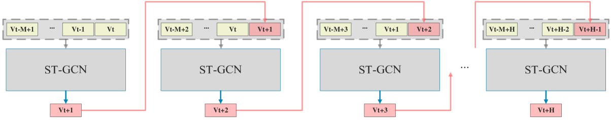
Figure 2: Sequence of ST-GCN predictions for future time steps. In each step, the output of the current state is used as the last input graph to predict the next timestep.

Visualization of Hidden Layer Representations All the results depicted in the t-SNE plots illustrate the hidden layer representation (which functions as the input to the output layer) for 50 test data points, each represented as an individual data instance, and is subsequently fed into t-SNE for visualization. In the plots, the red dots signify the student, while the blue dots represent either the teacher or the baseline pruning network (utilized exclusively for certain pruning results). The data employed in these visualizations is sourced from two datasets: PeMSD7 (depicted in Figure a) and PeMSD8 (depicted in Figure b). We can assess the effectiveness of our method by examining the t-SNE plots. In these visual representations, the proximity or overlap of the red and blue dots serves as an indicator of the model’s success. Ideally, when the method is effective, the red and blue dots should be close to or overlapping each other.

4.3 Evaluation Metrics and Training Details:

The results of traffic prediction in all tables are reported for the next 15, 30, and 45 minutes. The output values and calculated errors for these three time units are reported using three error functions: MAPE (Mean Absolute Percentage Error), MAE (Mean Absolute Error), and RMSE (Root Mean Square Error). The execution time reported in the tables are based on a batch of 1140 data and average over 100 runs.

4.4 Knowledge Distillation Analysis

All knowledge distillation experiments, except for pruning, employed the teacher and student models outlined in Table 1 and depicted in Figure 1 which provide comprehensive information on both networks, serving as a reference for subsequent comparisons and analysis. In the table, the column labeled ’Hidden Blocks Channel’ represents the channels for each spatial and temporal layer in the two hidden blocks of the ST-GCN network. For a more detailed explanation, we have visualized these channels on each layer in the accompanying Figure. Additionally, the columns: ”Test Time (s),” denotes the average test time over 100 trials, and ”FLOPS,” indicating the network’s floating-point operations per second (FLOPS) on a single forward pass. The student to teacher parameter ratio is approximately $3\%$ in both datasets. The execution time of the student network has reduced by approximately $83\%-84\%$ compared to the teacher. The number of blocks and layers in both networks is the same, and the difference in the number of parameters is due to the variation in the number of channels in each layer. The FLOPS ratio of the student network to the teacher is approximately $4\%$ for the PeMSD7 dataset and $2.5\%$ for the PeMSD8 dataset. We compared our proposed loss function, $L_{\text{ORD}}$, with other knowledge distillation loss functions such as $L_{\text{RD(KL)}}$, $L_{\text{RD(L2)}}$ [27, 28, 30, 29, 25]. The results are shown in Table 2. In all cases, except one (15-minute prediction on the PeMSD7 dataset), our approach has shown improvement compared to other approaches. For PeMSD7, $L_{\text{ORD}}$(ours) demonstrates competitive performance compared to $L_{\text{RD(L2)}}$ and $L_{\text{RD(KL)}}$ across all evaluated metrics. $L_{\text{ORD}}$(ours) consistently outperforming both $L_{\text{RD(L2)}}$ and $L_{\text{RD(KL)}}$ in MAE and RMSE for 15 min and 30 min predictions. This highlights the effectiveness of the overseen knowledge distillation method in capturing underlying patterns and improving accuracy. In the case of PeMSD8, $L_{\text{ORD}}$(ours) exhibits clear advantages over $L_{\text{RD(L2)}}$ and $L_{\text{RD(KL)}}$ in various metrics. Specifically, for MAE and RMSE at 15 min and 30 min prediction intervals, it consistently achieves lower errors, indicating superior predictive capabilities.

Table 2: Comparison of our approach $L_{\text{ORD}}$ with $L_{\text{RD(L2)}}$ and $L_{\text{RD(KL)}}$ on PeMSD7 and PeMSD8

   PeMSD7 Models MAPE MAE RMSE 15 min 30 min 45 min 15 min 30 min 45 min 15 min 30 min 45 min Teacher 5.223 7.316 8.739 2.230 3.010 3.565 4.097 5.752 6.834 Student W/O KD 6.423 9.685 12.298 2.666 3.868 4.799 4.649 6.938 8.610 Student $L_{\text{RD(L2)}}$ 6.379 9.661 12.474 2.768 4.214 5.527 4.709 7.185 9.178 Student $L_{\text{RD(KL)}}$ 6.411 9.527 11.894 2.700 3.938 4.918 4.672 6.984 8.657 Student $L_{\text{ORD}}$(ours) 6.411 9.516 12.104 2.762 4.091 5.221 4.645 6.847 8.569

   PeMSD8 Models MAPE MAE RMSE 15 min 30 min 45 min 15 min 30 min 45 min 15 min 30 min 45 min Teacher 2.293 3.239 3.925 1.211 1.665 2.031 2.524 3.501 4.081 Student W/O KD 2.967 4.035 4.734 1.472 1.956 2.294 2.988 4.090 4.706 Student $L_{\text{RD(L2)}}$ 2.812 3.976 4.908 1.426 1.953 2.387 2.839 3.978 4.733 Student $L_{\text{RD(KL)}}$ 2.964 4.179 5.057 1.507 2.125 2.575 2.895 3.971 4.664 Student $L_{\text{ORD}}$(ours) 2.661 3.717 4.553 1.363 1.885 2.285 2.788 3.862 4.573

We conducted a comparative analysis of our final loss function, $L_{\text{STCD}}$, against other approaches [27, 28, 30, 29, 25], and the results are presented in Table 4 and Figure 3. By reviewing the table, for PeMSD7, $L_{\text{STCD}}$(ours) demonstrates significant improvements over the baseline Student W/O KD and outperforms other knowledge distillation methods, including $L_{\text{RD(L2)}}$, $L_{\text{RD(KL)}}$, and SKD. Specifically, in terms of MAE and RMSE for the 15-minute and 30-minute predictions, $L_{\text{STCD}}$(ours) consistently achieves lower errors. Similarly, on the PeMSD8 dataset, $L_{\text{STCD}}$(ours) exhibits superior performance across various metrics when compared to $L_{\text{RD(L2)}}$, $L_{\text{RD(KL)}}$, and SKD. Noteworthy is the consistent outperformance in MAE and RMSE at the 15-minute and 30-minute prediction intervals, emphasizing the effectiveness of $L_{\text{STCD}}$(ours) in capturing spatial-temporal dependencies and enhancing predictive accuracy. These findings highlight the efficacy of the $L_{\text{STCD}}$(ours) approach, underscoring its potential as a robust spatial-temporal loss function for knowledge distillation in the context of traffic flow prediction datasets. Figure 3 illustrates better convergence and pattern imitation of the $L_{\text{STCD}}$ approach compared to other approaches in both knowledge bases. Additionally, we report the ratio of attention to teacher output instead of the dataset target in Table 3.

Table 3: Ratios of attention to teacher prediction to all training data

   Models Ratios of Attention to Teacher Prediction PeMSD7 PeMSD8 Student $L_{\text{ORD}}$ 3.009% 0.749% Student $L_{\text{SCD}}$ 1.377% 0.046% Student $L_{\text{TCD}}$ 64.637% 0.503% Student $L_{\text{STCD}}$ 15.844% 0.103%

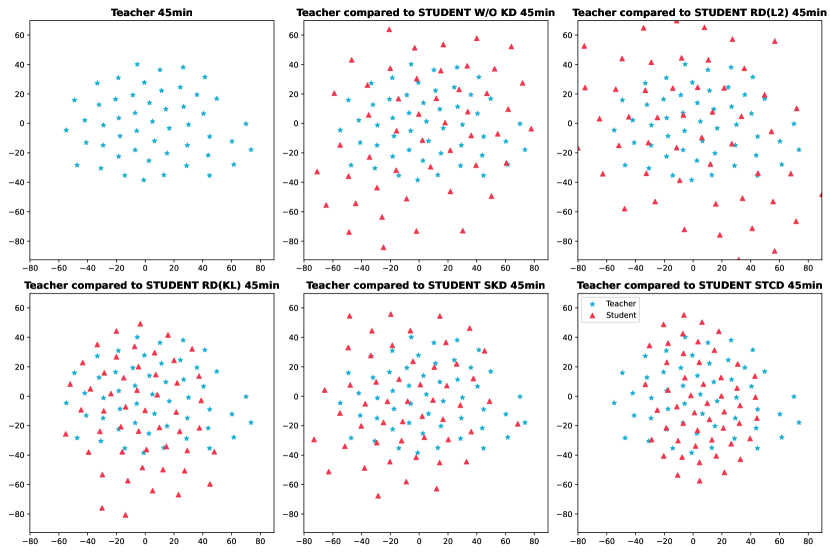
(a) PeMSD7

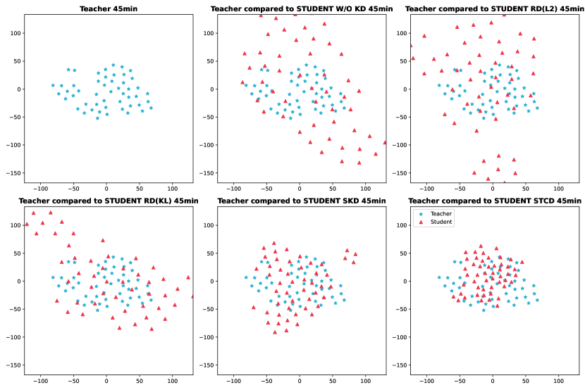
(b) PeMSD8

Figure 3: Comparison of our spatial-temporal correlation distillation loss function $L_{\text{STCD}}$ with the $L_{\text{RD(L2)}}$, $L_{\text{RD(KL)}}$ and $L_{\text{SKD}}$ loss functions. Subfigure 3(a) shows results for PeMSD7 dataset, and Subfigure 3(b) shows for PeMSD8. The left chart in the top row corresponds to the teacher, while the middle chart in the top row pertains to a student without knowledge distillation. In the second row, the right chart represents our loss function, and the other charts indicate different loss functions.

Table 4: Performance comparison of our spatial-temporal correlation distillation loss function $L_{\text{STCD}}$ with other loss functions

   PeMSD7 Models MAPE MAE RMSE 15 min 30 min 45 min 15 min 30 min 45 min 15 min 30 min 45 min Teacher 5.223 7.316 8.739 2.230 3.010 3.565 4.097 5.752 6.834 Student W/O KD 6.423 9.685 12.298 2.666 3.868 4.799 4.649 6.938 8.610 Student $L_{\text{RD(L2)}}$ 6.379 9.661 12.474 2.768 4.214 5.527 4.709 7.185 9.178 Student $L_{\text{RD(KL)}}$ 6.411 9.527 11.894 2.700 3.938 4.918 4.672 6.984 8.657 Student $L_{\text{SKD}}$ 6.282 9.503 11.902 2.762 4.092 5.101 4.735 7.161 8.923 Student $L_{\text{STCD}}$(ours) 6.078 9.043 11.488 2.615 3.776 4.754 4.537 6.678 8.344

   PeMSD8 Models MAPE MAE RMSE 15 min 30 min 45 min 15 min 30 min 45 min 15 min 30 min 45 min Teacher 2.293 3.239 3.925 1.211 1.665 2.031 2.524 3.501 4.081 Student W/O KD 2.967 4.035 4.734 1.472 1.956 2.294 2.988 4.090 4.706 Student $L_{\text{RD(L2)}}$ 2.812 3.976 4.908 1.426 1.953 2.387 2.839 3.978 4.733 Student $L_{\text{RD(KL)}}$ 2.964 4.179 5.057 1.507 2.125 2.575 2.895 3.971 4.664 Student $L_{\text{SKD}}$ 2.726 3.819 4.553 1.409 1.944 2.317 2.909 4.139 4.894 Student $L_{\text{STCD}}$(ours) 2.491 3.375 4.067 1.281 1.719 2.052 2.716 3.707 4.385

Ablation Study Finally, we conducted an ablation study on the $L_{\text{STCD}}$ loss function, and the results are presented in Table 5. In PeMSD7, comparing various knowledge distillation models, $L_{\text{STCD}}$(ours) exhibits competitive performance against other variants, including $L_{\text{ORD}}$, $L_{\text{TCD}}$, and $L_{\text{SCD}}$. For instance, in terms of Mean Absolute Percentage Error (MAPE), Mean Absolute Error (MAE), and Root Mean Squared Error (RMSE) at different predictions (15 min, 30 min, and 45 min), $L_{\text{STCD}}$(ours) consistently demonstrates effectiveness in achieving lower errors compared to the baseline Student W/O KD and other knowledge distillation methods. Moving to the PeMSD8 dataset, the results in Table 5 further emphasize the robust performance of $L_{\text{STCD}}$(ours). When compared to $L_{\text{ORD}}$, $L_{\text{TCD}}$, and $L_{\text{SCD}}$, $L_{\text{STCD}}$(ours) consistently achieves lower MAPE, MAE, and RMSE across various predictions. Specifically, at 15 min and 30 min intervals, $L_{\text{STCD}}$(ours) outperforms its counterparts, showcasing its efficacy in capturing spatial-temporal dependencies and enhancing predictive accuracy.

Table 5: Results from the ablation study comparing the impact of individual loss functions ( $L_{\text{SCD}}$, $L_{\text{TCD}}$, and $L_{\text{ORD}}$ ), contributing to the construction of our overall $L_{\text{STCD}}$ loss function.

   PeMSD7 Models MAPE MAE RMSE 15 min 30 min 45 min 15 min 30 min 45 min 15 min 30 min 45 min Teacher 5.223 7.316 8.739 2.230 3.010 3.565 4.097 5.752 6.834 Student W/O KD 6.423 9.685 12.298 2.666 3.868 4.799 4.649 6.938 8.610 Student $L_{\text{ORD}}$ 6.411 9.516 12.104 2.762 4.091 5.221 4.645 6.847 8.569 Student $L_{\text{TCD}}$ 6.320 9.411 11.667 2.730 3.966 4.853 4.678 6.899 8.512 Student $L_{\text{SCD}}$ 6.326 9.193 11.380 2.743 3.957 4.866 4.645 6.853 8.476 Student $L_{\text{STCD}}$ 6.078 9.043 11.488 2.615 3.776 4.754 4.537 6.678 8.344

   PeMSD8 Models MAPE MAE RMSE 15 min 30 min 45 min 15 min 30 min 45 min 15 min 30 min 45 min Teacher 2.293 3.239 3.925 1.211 1.665 2.031 2.524 3.501 4.081 Student W/O KD 2.967 4.035 4.734 1.472 1.956 2.294 2.988 4.090 4.706 Student $L_{\text{ORD}}$ 2.661 3.717 4.553 1.363 1.885 2.285 2.788 3.862 4.573 Student $L_{\text{TCD}}$ 2.509 3.497 4.215 1.296 1.747 2.063 2.665 3.716 4.406 Student $L_{\text{SCD}}$ 2.619 3.680 4.457 1.355 1.850 2.214 2.722 3.778 4.478 Student $L_{\text{STCD}}$ 2.491 3.375 4.067 1.281 1.719 2.052 2.716 3.707 4.385

4.4.1 Hyperparameters

You can refer to Tables 6 for the learning rate, batch size, and hyperparameters related to knowledge distillation. These parameters are crucial in shaping the behavior of the models during training. In the context of the provided equations, the ”Models” column enumerates various knowledge distillation approaches evaluated for PeMSD7 and PeMSD8 datasets. Each approach, such as $L_{\text{RD(L2)}}$, $L_{\text{RD(KL)}}$, $L_{\text{SKD}}$, $L_{\text{ORD}}$(ours), and $L_{\text{STCD}}$(ours), incorporates distinct strategies for transferring knowledge. The ”Batch Size” column indicates the number of training samples utilized in each iteration for a specific model and dataset. For instance, SKD employs a batch size of 16 for PeMSD7 and 60 for PeMSD8. $L_{\text{RD(L2)}}$, $L_{\text{RD(KL)}}$, $L_{\text{ORD}}$(ours), and $L_{\text{STCD}}$(ours) maintain a batch size of 50 for both datasets, influencing the granularity of parameter updates during training. The ”Learning Rate” column specifies the step size during optimization, impacting the convergence of the models. Across various models and datasets, a learning rate of 1E-03 is consistently chosen, except for SKD on PeMSD8, which employs a learning rate of 1E-02. This parameter governs the size of the steps taken to reach a minimum in the loss landscape. The hyperparameters $\alpha_{1},\alpha_{2},\alpha_{3},\alpha,$ and $\beta$ are pivotal in the knowledge distillation process, as defined in equations (6), (11), (2), and (3). These values determine the contributions of different loss terms and the overall weighting of knowledge distillation components. For instance, $\alpha_{1}$ in $L_{\text{ORD}}$(ours) plays a role in deciding whether to prioritize teacher predictions or target labels based on a threshold.

Table 6: Hyperparameters of the proposed knowledge distillation loss functions

   PeMSD7 Models Batch Size Learning Rate $\alpha$1 $\alpha$2 $\alpha$3 $\alpha$ $\beta$ $L_{\text{RD(L2)}}$ 50 1E-03 - - - - 0.045 $L_{\text{RD(KL)}}$ 50 1E-03 - - - - 0.007 $L_{\text{SKD}}$ 16 1E-03 - - - 0.333 - $L_{\text{ORD}}$(ours) 50 1E-03 0.593 - - - - $L_{\text{STCD}}$(ours) 50 1E-03 0.170 0.047 0.313 - -

   PeMSD8 Models Batch Size Learning Rate $\alpha$1 $\alpha$2 $\alpha$3 $\alpha$ $\beta$ $L_{\text{RD(L2)}}$ 50 1E-03 - - - - 0.905 $L_{\text{RD(KL)}}$ 50 1E-03 - - - - 0.728 $L_{\text{SKD}}$ 60 1E-02 - - - 0.005 - $L_{\text{ORD}}$(ours) 50 1E-03 0.541 - - - - $L_{\text{STCD}}$(ours) 50 1E-03 0.846 0.465 0.504 - -

4.5 Pruning and Fine-Tuning Analysis

In this section, the focus is on modifying the student network through a pruning algorithm, intentionally applying the same algorithm to the teacher network. The objective is to create a student network with parameters comparable to the one used in knowledge distillation experiments. The goal is to showcase that a consciously pruned student network, guided by Algorithm 1, exhibits superior learning capabilities compared to a predetermined student network used in knowledge distillation. The experiment’s outcomes are summarized in Table 7 and Figures 4 and 5.

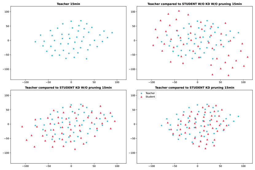
(a) PeMSD7

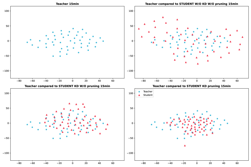
(b) PeMSD8

Figure 4: Results illustrating the impact of employing the pruning algorithm to enhance knowledge distillation. Subfigure 4(a) shows results for PeMSD7 dataset, and Subfigure 4(b) shows for PeMSD8. The left chart in the top row corresponds to the teacher, while the right chart in the top row pertains to a student without knowledge distillation and without pruning. In the second row, the left chart represents a student with knowledge distillation but without pruning, and the right chart represents a student with both knowledge distillation and pruning.

Table 7: The results showcase the impact of applying the pruning algorithm in enhancing knowledge distillation.

   PeMSD7 Models Parameter $\%$ MAPE MAE RMSE 15 min 30 min 45 min 15 min 30 min 45 min 15 min 30 min 45 min Teacher $100\%$ 5.223 7.316 8.739 2.230 3.010 3.565 4.097 5.752 6.834 Student W/O pruning algorithm $~{}3\%$ 6.078 9.043 11.488 2.615 3.776 4.754 4.537 6.678 8.344 Student W pruning algorithm $~{}3\%$ 6.148 9.026 11.506 2.563 3.694 4.754 4.398 6.485 8.228

   PeMSD8 Models Parameter $\%$ MAPE MAE RMSE 15 min 30 min 45 min 15 min 30 min 45 min 15 min 30 min 45 min Teacher $100\%$ 2.293 3.239 3.925 1.211 1.665 2.031 2.524 3.501 4.081 Student W/O pruning algorithm $~{}3\%$ 2.491 3.375 4.067 1.281 1.719 2.052 2.716 3.707 4.385 Student W pruning algorithm $~{}3\%$ 2.379 3.307 3.961 1.248 1.679 1.990 2.597 3.594 4.193

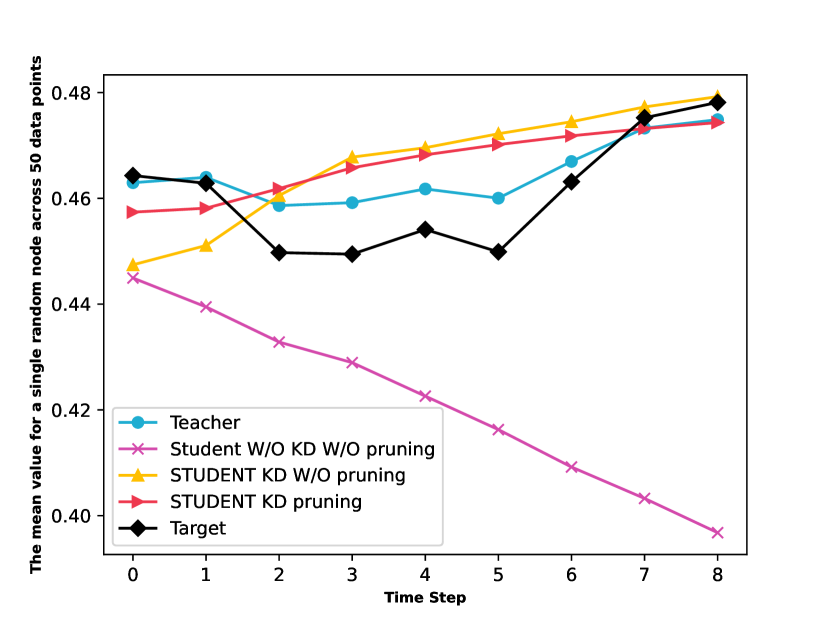
(a) PeMSD7

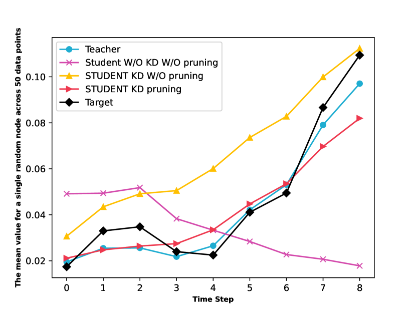
(b) PeMSD8

Figure 5: The results highlight the impact of employing the pruning algorithm, demonstrating the average predicted value for a randomly selected node based on 50 data points.

Table 7 presents results comparing the performance of the student network with and without pruning through knowledge distillation. Looking at the PeMSD7 dataset in the table, the teacher model, using all of its parameters, achieved an RMSE of 4.097 for a 15-minute prediction. On the other hand, the student model without the pruning algorithm, which retained about 3$\%$ of the parameters, had a higher RMSE of 4.537 for the same prediction period. However, when we applied the pruning algorithm to the student model (also retaining 3$\%$ of parameters), the RMSE improved to 4.398. This improvement highlights how pruning positively influences knowledge distillation by refining the student model’s predictive performance. A significant improvement is observed in the PeMSD8 dataset. The teacher model achieved a 15-minute MAPE of 2.293 with 100$\%$ of its parameters. In contrast, the student model without pruning, retaining approximately 3$\%$ of the parameters, had a 15-minute MAPE of 2.491. The application of the pruning algorithm to the student model (also retaining 3$\%$ of parameters) resulted in a decreased 15-minute MAPE of 2.379. These results vividly demonstrate that the pruning algorithm significantly contributes to enhancing knowledge distillation, showcasing instances where pruning leads to better model performance compared to the non-pruned counterparts. The improvements in MAPE values indicate that the pruning algorithm helps the student models better capture the knowledge from the teacher model. Figure 4 visually represents the performance enhancement achieved by the pruning algorithm, showing the average predicted values for a random node on 50 training data points.
Next, we conduct a comparative analysis between the presented pruning algorithm and a non-distillation scenario from [6]. Previous research has confirmed that incorporating knowledge distillation enhances accuracy while utilizing a more straightforward model. Building upon this, our current study extends the concept, illustrating that Algorithm 1 yields a student architecture that performs better during training with KD. We compare Algorithm 1 with [6] using a base pruning model from Table 1. The results depicted in Table 8 underscore that our pruning algorithm consistently outperforms the alternative across various pruning percentages.

Table 8: Comparison of the performance between Algorithm 1 and the pruning algorithm that does not utilize knowledge distillation.

   PeMSD7 Models Parameter $\%$ MAPE MAE RMSE 15 min 30 min 45 min 15 min 30 min 45 min 15 min 30 min 45 min Base Model $100\%$ 5.512 8.004 9.988 2.321 3.216 3.896 4.177 6.006 7.341 Pruned W/O KD $25\%$ 6.185 8.981 11.060 2.721 3.889 4.728 4.682 6.947 8.579 Pruned W $L_{\text{STCD}}$(ours) $25\%$ 5.950 8.654 10.906 2.544 3.705 4.751 4.406 6.424 8.014 Pruned W/O KD $50\%$ 6.571 9.735 12.114 2.975 4.389 5.418 4.858 7.255 8.971 Pruned W $L_{\text{STCD}}$(ours) $50\%$ 6.232 9.185 11.419 2.584 3.773 4.723 4.524 6.773 8.448 Pruned W/O KD $75\%$ 7.090 11.746 15.940 2.925 4.635 6.034 4.943 7.759 9.967 Pruned W $L_{\text{STCD}}$(ours) $75\%$ 6.275 9.436 12.261 2.644 3.783 4.708 4.586 6.680 8.270

   PeMSD8 Models Parameter $\%$ MAPE MAE RMSE 15 min 30 min 45 min 15 min 30 min 45 min 15 min 30 min 45 min Base Model $100\%$ 2.206 3.028 3.677 1.187 1.592 1.924 2.479 3.434 4.084 Pruned W/O KD $25\%$ 2.438 3.459 4.338 1.279 1.781 2.227 2.615 3.644 4.359 Pruned W $L_{\text{STCD}}$(ours) $25\%$ 2.427 3.200 3.782 1.236 1.630 1.927 2.672 3.645 4.303 Pruned W/O KD $50\%$ 2.456 3.514 4.449 1.322 1.890 2.397 2.648 3.797 4.685 Pruned W $L_{\text{STCD}}$(ours) $50\%$ 2.424 3.310 3.988 1.261 1.693 2.029 2.605 3.550 4.169 Pruned W/O KD $75\%$ 2.530 3.503 4.275 1.335 1.823 2.225 2.715 3.810 4.596 Pruned W $L_{\text{STCD}}$(ours) $75\%$ 2.348 3.192 3.788 1.228 1.627 1.911 2.595 3.577 4.216

In the PeMSD7 dataset, our proposed pruned W $L_{\text{STCD}}$ (pruned with $L_{\text{STCD}}$) consistently exhibits superior performance compared to the pruned W/O KD (without knowledge distillation) approach. This superiority is evident in metrics such as mean absolute percentage error (MAPE), mean absolute error (MAE), and root mean square error (RMSE) across different time intervals (15 min, 30 min, and 45 min). For example, at a pruning level of $25\%$, pruned W $L_{\text{STCD}}$ achieves lower MAPE values (5.950, 8.654, 10.906) compared to pruned W/O KD (6.185, 8.981, 11.060) for 15 min, 30 min, and 45 min intervals, respectively. Similar trends are observed at higher pruning levels of $50\%$ and $75\%$, where pruned W $L_{\text{STCD}}$ consistently outperforms pruned W/O KD across all evaluation metrics. The superiority of our algorithm is further emphasized in the PeMSD8 dataset. At various pruning levels, pruned W $L_{\text{STCD}}$ consistently records lower MAPE, MAE, and RMSE values compared to pruned W/O KD. Remarkably, even at aggressive pruning levels of $75\%$, pruned W $L_{\text{STCD}}$ maintains competitive performance, showcasing the effectiveness and robustness of our proposed pruning algorithm. Overall, the findings affirm that our introduced pruning algorithm plays a pivotal role in enhancing learning through knowledge distillation, significantly improving neural network accuracy by employing fewer parameters and simpler structures. In the executions related to comparing our pruning algorithm with the one presented in [6], pruning operations are performed after every two cycles, and the final network cycle undergoes fine-tuning (see Table 8).

4.5.1 Hyperparameters

The hyperparameters for the proposed pruning algorithm are presented in Table 9. The table categorizes hyperparameters based on the percentage of pruning applied, as well as batch size, learning rate, and three alpha values ($\alpha_{1}$, $\alpha_{2}$, and $\alpha_{3}$), specific to the PeMSD7 and PeMSD8 datasets. For instance, in the PeMSD7 row with a pruning percentage of $97\%$, only $3\%$ of the model parameters are retained. The associated hyperparameters include a batch size of 25, a learning rate of $1\times 10^{-3}$, and alpha values $\alpha_{1}=0.099$, $\alpha_{2}=0.091$, and $\alpha_{3}=0.531$. The alpha values play distinct roles in the loss function equations. For $\alpha_{1}$, it defines the conditions under which different loss terms are applied in $L_{\text{ORD}}$ as specified in Equation 6. Meanwhile, $\alpha_{2}$ and $\alpha_{3}$ are used as weights in Equation 11, influencing the contributions of $L_{\text{SCD}}$ and $L_{\text{TCD}}$ relative to $L_{\text{ORD}}$.

Table 9: Hyperparameters of the proposed pruning algorithm

   PeMSD7 Pruned $\%$ Batch Size Learning Rate $\alpha$1 $\alpha$2 $\alpha$3 97$\%$ 25 1E-03 0.099 0.091 0.531 75$\%$ 50 1E-03 0.963 0.716 0.081 50$\%$ 50 1E-03 0.935 0.981 0.129 25$\%$ 50 1E-03 0.971 0.234 0.684

   PeMSD8 Pruned $\%$ Batch Size Learning Rate $\alpha$1 $\alpha$2 $\alpha$3 97$\%$ 25 1E-03 0.746 0.445 0.020 75$\%$ 50 1E-03 0.996 0.720 0.405 50$\%$ 50 1E-03 0.946 0.516 0.094 25$\%$ 50 1E-03 0.748 0.324 0.868

5 Conclusion and Future Works

5.1 Conclusion

We addressed the critical challenge of predicting traffic conditions to reduce transportation time. Our chosen methodology involved leveraging the spatio-temporal graph convolutional network (ST-GCN) for processing traffic prediction data, and we proposed a solution to improve the execution time of ST-GCNs. This involved introducing a novel approach that employed knowledge distillation to train a smaller network (referred to as the student) using distilled data from a more complex network (referred to as the teacher), all while maintaining a high level of prediction accuracy. Additionally, we tackled the challenge of determining the architecture of the student network within the knowledge distillation process, employing Algorithm 1. Our findings demonstrated that a student network derived through Algorithm 1 exhibited enhanced performance during the knowledge distillation training process. Furthermore, by utilizing a simpler model in knowledge distillation, as opposed to the teacher model, as the base model in pruning, we illustrated that the performance of our algorithm was not necessarily contingent on the high accuracy of the base model. We evaluated our proposed concepts using two real-world datasets, PeMSD7 and PeMSD8, demonstrating the effectiveness of our approach in predicting traffic conditions. Overall, our research contributed to the field by presenting a methodology to optimize the execution time of spatio-temporal graph convolutional networks for traffic prediction without compromising accuracy.

5.2 Future Works

As we progress, we have the opportunity to explore our cost function $L_{\text{STCD}}$ and Algorithm 1 on alternative spatiotemporal graph neural networks, such as ASTGCN. Furthermore, considering the method proposed in [32] and [26], we can explore whether using multiple teachers in Algorithm 1 and knowledge distillation with $L_{\text{STCD}}$ can lead to a model with higher accuracy. Alternatively, we can develop a model capable of executing the tasks performed by all its teachers with increased accuracy and reduced execution time compared to the model in [26]. It is possible to enhance the concept of knowledge distillation based on the cost function $L_{\text{STCD}}$ by incorporating relationship-based approaches. This improvement allows for the consideration of student and teacher networks with varying numbers of layers.

References

- [1] B Yu; H Yin; Z Zhu, Spatio-Temporal Graph Convolutional Networks: A Deep Learning Framework for Traffic Forecasting, 27th International Joint Conference on Artificial Intelligence, 2018.
- [2] D. A. Tedjopurnomo; Z. Bao; B. Zheng; F. M. Choudhury; A. K. Qin, A Survey on Modern Deep Neural Network for Traffic Prediction: Trends, Methods and Challenges, IEEE Transactions on Knowledge and Data Engineering, 2022.
- [3] S Guo; Y Lin; N Feng; C Song; H Wan, Attention Based Spatial-Temporal Graph Convolutional Networks for Traffic Flow Forecasting, AAAI conference on artificial intelligence, 2019.
- [4] G Hinton; O Vinyals; J Dean, Distilling the Knowledge in a Neural Network, NIPS 2014 Deep Learning Workshop, 2015.
- [5] Y LeCun; J Denker; S Solla, Optimal Brain Damage, Advances in Neural Information Processing Systems 2 (NIPS 1989), 1989.
- [6] P Molchanov; A Mallya; S Tyree; I Frosio; J Kautz, Importance estimation for neural network pruning, IEEE/CVF conference on computer vision and pattern recognition. 2019, 2019.
- [7] Shengjie Min; Zhan Gao; Jing Peng; Liang Wang; Ke Qin; Bo Fang, STGSN — A Spatial–Temporal Graph Neural Network framework for time-evolving social networks, Knowledge-Based Systems, 2021.
- [8] Jianping Gou; Baosheng Yu; Stephen John Maybank; Dacheng Tao, Knowledge Distillation: A Survey, International Journal of Computer Vision (2021), 2021.
- [9] Yu Cheng; Duo Wang; Pan Zhou; Tao Zhang, A Survey of Model Compression and Acceleration for Deep Neural Networks, IEEE Signal Processing Magazine, 2020.
- [10] J. Yim; D. Joo; J. Bae and J. Kim, A Gift from Knowledge Distillation: Fast Optimization, Network Minimization and Transfer Learning, 2017 IEEE Conference on Computer Vision and Pattern Recognition (CVPR), 2017.
- [11] G Chen; W Choi; X Yu; T Han, Learning efficient object detection models with knowledge distillation, Neural Information Processing Systems 30 (NIPS 2017), 2017.
- [12] Feng Zhang; Xiatian Zhu; Mao Ye, Fast Human Pose Estimation, Computer Vision and Pattern Recognition (CVPR2019), 2019 .
- [13] Zhong Meng; Jinyu Li; Yong Zhao; Yifan Gong, Conditional Teacher-Student Learning, , 2019 .
- [14] Yoshua Bengio; Aaron Courville; Pascal Vincent, Representation learning: A review and new perspectives, , 2013.
- [15] Peyman Passban; Yimeng Wu; Mehdi Rezagholizadeh; Qun Liu, ALP-KD: Attention-Based Layer Projection for Knowledge Distillation , AAAI 2021, 2021.
- [16] X Wang; T Fu; S Liao; S Wang; Z Lei; T Mei, Exclusivity-consistency regularized knowledge distillation for face recognition , Computer Vision–ECCV 2020, 2020 .
- [17] Seung Hyun Lee; Dae Ha Kim; Byung Cheol Song, Self-supervised Knowledge Distillation Using Singular Value Decomposition, ECCV 2018, 2018 .
- [18] Umar Asif; Jianbin Tang; Stefan Harrer, Ensemble Knowledge Distillation for Learning Improved and Efficient Networks, Computer Vision and Pattern Recognition (cs.CV); Machine Learning (cs.LG), 2020.
- [19] Seyed-Iman Mirzadeh; Mehrdad Farajtabar; Ang Li; Nir Levine; Akihiro Matsukawa; Hassan Ghasemzadeh, Improved knowledge distillation via teacher assistant, AAAI 2020, 2020.
- [20] Hossein Mobahi; Mehrdad Farajtabar; Peter L. Bartlett, Self-Distillation Amplifies Regularization in Hilbert Space , , 2020.
- [21] Wen W; Wu C; Wang Y; Chen Y; Li H, Learning structured sparsity in deep neural networks, Neural Information Processing Systems (NIPS), IEEE, 2016.
- [22] N. Ramakrishnan; T. Soni, Network Traffic Prediction Using Recurrent Neural Networks, 2018 17th IEEE International Conference on Machine Learning and Applications (ICMLA), 2018.
- [23] Tang, Jinjun; Abduljabbar, Rusul L; Dia, Hussein; Tsai, Pei-Wei, Unidirectional and Bidirectional LSTM Models for Short-Term Traffic Prediction, Journal of Advanced Transportation, 2021.
- [24] Yaguang Li; Rose Yu; Cyrus Shahabi; Yan Liu, Diffusion Convolutional Recurrent Neural Network: Data-Driven Traffic Forecasting, ICLR 2018, 2018.
- [25] Y. Yang; J. Qiu; M. Song; D. Tao; X. Wang, Distilling Knowledge from Graph Convolutional Networks, 2020 IEEE/CVF Conference on Computer Vision and Pattern Recognition (CVPR), 2020.
- [26] Y Jing; Y Yang; X Wang; M Song, Amalgamating Knowledge from Heterogeneous Graph Neural Networks, 2021 IEEE/CVF Conference on Computer Vision and Pattern Recognition (CVPR), 2021.
- [27] C. Bian; W. Feng; L. Wan; S. Wang, Structural knowledge distillation for efficient skeleton-based action recognition, IEEE Transactions on Image Processing, 2021.
- [28] Z Huang; N Wang, Like What You Like: Knowledge Distill via Neuron Selectivity Transfer, Computer Vision and Pattern Recognition (cs.CV); Machine Learning (cs.LG); Neural and Evolutionary Computing (cs.NE), 2017.
- [29] Adriana Romero; Nicolas Ballas; Samira Ebrahimi Kahou; Antoine Chassang; Carlo Gatta; Yoshua Bengio, FitNets: Hints for Thin Deep Nets, Machine Learning (cs.LG); Neural and Evolutionary Computing (cs.NE), 2014.
- [30] Sergey Zagoruyko; Nikos Komodakis, Paying More Attention to Attention: Improving the Performance of Convolutional Neural Networks via Attention Transfer, Computer Vision and Pattern Recognition (cs.CV), 2017.
- [31] Cheng Yang; Jiawei Liu; Chuan Shi, Extract the Knowledge of Graph Neural Networks and Go Beyond it: An Effective Knowledge Distillation Framework, Machine Learning (cs.LG); Social and Information Networks (cs.SI), 2021.
- [32] Sihui Luo; Xinchao Wang; Gongfan Fang; Yao Hu; Dapeng Tao; Mingli Song, Knowledge Amalgamation from Heterogeneous Networks by Common Feature Learning, the 28th International Joint Conference on Artificial Intelligence (IJCAI 2019), 2019.