The hidden companion in J1527: a 0.69 solar-mass white dwarf?

Abstract

Finding nearby neutron stars can probe the supernova and metal-enrichment histories near our Solar system. Recently, Lin et al. (2023) reported an exciting neutron star candidate, 2MASS J15274848+3536572 (hereafter J1527), with a small Gaia distance of 118 parsecs. They claim that J1527 harbors an unseen neutron star candidate with an unusually low mass of $0.98\pm 0.03\,M_{\odot}$. In this work, we use the Canada-France-Hawaii Telescope high-resolution spectrum to measure J1527’s orbital inclination independently. Our spectral fitting suggests an orbital inclination of $63\pm 2$ degrees. Instead, by fitting a complex hybrid variability model consisting of the ellipsoidal-variation component and the star-spot modulation to the observed light curve, Lin et al. (2023) obtains an orbital inclination of $45.2_{-0.20}^{+0.13}$ degrees. We speculate that the orbital inclination obtained by the light-curve fitting is underestimated since J1527’s light curves are obviously not pure ellipsoidal variations. According to our new inclination ($i\sim 63$ degrees), the mass of the unseen compact object is reduced to $0.69\pm 0.02$ $M_{\odot}$, which is as massive as a typical white dwarf.

1 Introduction

The identification of compact objects plays a crucial role in several research areas, including understanding the metal enrichment process in the Milky Way, studying the evolution of single stars and binary systems, and exploring the impacts of nearby supernova explosions on the solar system environment. Theoretical predictions suggest that there may be hundreds of millions of neutron stars (NSs) in the Milky Way (e.g. Camenzind, 2007). However, only a few thousand NSs have been found, primarily through radio pulses, and some through X-ray outbursts (Özel & Freire, 2016). The number of discoveries is far less than the theoretical expectations. The reason could be that the vast majority of NSs have weak electromagnetic radiation characteristics and are difficult to detect directly. To search for more compact objects in quiescent states, a series of works have been done based on spectroscopic or photometric time-domain surveys (e.g. Yi et al., 2019; Zheng et al., 2022; Yuan et al., 2022; Mu et al., 2022; Mazeh et al., 2022; El-Badry et al., 2023). These studies indirectly identify compact objects by analyzing the dynamical properties of companion stars in binary systems that contain unseen compact objects.

An increase of radionuclide element iron-60 (${}^{60}\mathrm{Fe}$; half-life, 2 million years) has been detected in a sample of Pacific Ocean crust (e.g., Koll et al., 2019; Wallner et al., 2021). This evidence suggests that several nearby supernovae occurred within millions of years in the vicinity of the solar system. Observations have also revealed the existence of a local bubble (a low-density cavity of the ISM) surrounding the solar system (Smith & Cox, 2001; Berghöfer & Breitschwerdt, 2002; Schulreich et al., 2017), further supporting the existence of nearby supernova events. Hence, it is of great interest to find the potential remnants, e.g., nearby NSs, of these events. Recent efforts in this regard include the studies of Zheng et al. (2022) and Lin et al. (2023). Zheng et al. (2022) discovered an NS candidate, J2354, located approximately 128 parsecs away from the solar system, in which the unseen compact object has a mass of $1.4\sim 1.6\,M_{\odot}$. In the work of Lin et al. (2023), the authors claim to have identified a binary system, J1527, located 118 parsecs from the solar system, with an unseen neutron star candidate of approximately 0.98$M_{\odot}$.

The mass function of the invisible star in J1527 is calculated to be 0.131 $M_{\odot}$, with the visible star being a K-type dwarf. To measure the mass of the unseen companion, it is vital to measure the inclination angle ($i$) of the binary. The inclination angle can be measured via two independent methods. The first method (for details, see, e.g., Zheng et al. 2022 and our Section 3) is to use high-resolution (e.g., $R>10,000$) spectra to measure the projected rotation broaden velocity, $V_{\mathrm{rot}}\sin i$ (hereafter $v\sin i$), of the visible star. If the visible star is tidally locked, $V_{\mathrm{rot}}={2\pi R_{1}}/{P_{\mathrm{orb}}}$, where $R_{1}$ is the visible star radius, and $P_{\mathrm{orb}}$ is the orbital period. The second method is to fit ellipsoidal modulations to the observed light curves. Lin et al. (2023) adopt the latter method to estimate the inclination of J1527, which is about 45 degrees. However, according to TESS observations, the flux variations of J1527 are not dominated by ellipsoidal variations and other mechanisms (e.g., spots) contribute significantly to the TESS light curve (see figure 6 in Lin et al. 2023). Hence, the inferred inclination angle in Lin et al. (2023) is questionable.

In this work, we aim to independently constrain the inclination angle of J1574 by measuring the projected rotation broaden velocity of the visible star. Hence, we performed a high-resolution spectral observation by using the Echelle SpectroPolarimetric Device for the Observation of Stars (ESPaDONs) mounted on the 3.6m optical/infrared telescope at Canada-France-Hawaii Observatory (CFHT). We show that the inclination estimate based on the light-curve fitting is biased, and the actual inclination is $63\pm 2$ degrees. As a result, the derived mass of the invisible compact object is significantly reduced to $0.69\pm 0.02$ $M_{\odot}$— the typical mass of a white dwarf (WD). In Section 2, we introduce the observation and data reduction. In Section 3, we describe the measurement process of $v\sin i$. The estimate of inclination and the compact object mass are provided in Section 4. Section 5 is the conclusion of this paper.

2 Observation

We observed J1527 twice using the ESPaDONs mounted on the CFHT telescope. The two observations were taken on 2023-07-09 and 2023-07-10, each executed with the “object+sky” spectroscopic mode and an exposure time of 660 seconds. The orbital phases of the two observations are 0.847 and 0.756, respectively (here, we define the phase zero point as the visible star being at superior conjunction). The first observation was conducted under bad weather conditions, rendering the signal-to-noise ratio (SNR) of the spectrum too low to utilize. The second observation yielded an SNR of 20 per pixel at 6,960 Å, a spectral resolution $R\approx 69,000$, and a wavelength coverage of $3,700-10,500$ Å. Therefore, we only use the second spectrum for subsequent analysis.

The CFHT spectra were reduced using an automatic pipeline known as Upena (https://www.cfht.hawaii.edu/Instruments/Upena/). This code performs bias and flat field corrections, cosmic-ray removal, wavelength calibration, sky subtraction, 1D spectrum extraction, and heliocentric radial velocity (RV) correction. The normalized “Star” flux reduced by Upena is used in our following measurements. We use the software LBLRTM (Clough et al., 1992, 2005; Gullikson et al., 2014) to model and correct the telluric absorption. The reduced spectrum is displayed in Figure 1, which shows evident broaden stellar absorption lines. Due to the relatively low SNR of the original spectrum, it is difficult to clearly distinguish the absorption line profile. We resample the original spectrum and show it in blue lines.

3 Measurements

To measure $v\sin i$, we create a synthetic stellar spectral grid for the interpolation of given stellar parameters, which include the effective temperature ($T_{\mathrm{eff}}$), surface gravity ($\log g$), and metallicities ($\mathrm{[M/H]}$). We employ the Turbospectrum (Plez, 2012) software to generate synthetic spectra for given stellar parameters. For atmospheric modeling, we use the 1-D plane-parallel LTE MARCS model atmospheres (Gustafsson et al., 2008). The dataset of atomic and molecular spectral lines are from Ryabchikova et al. (2015); Heiter et al. (2021). The macro-turbulence of the model is set at 2 $\mathrm{km\,s^{-1}}$. Because the rotational velocity of the visible star is significantly larger than this value, the macro-turbulence has a negligible impact on the fitting result. The wavelength interval of the synthetic spectra is set to 0.01Å. The temperature grid ranges from 2700 K to 8000 K, the $\log g$ grid spans from 2 to 5, and the grid for $\mathrm{[M/H]}$ ranges from -4 to 1. We employ the scipy.interpolate.RegularGridInterpolator function to execute high-dimensional interpolation on the spectral grid, thus enabling the acquisition of template spectra for a designated combination of $T_{\mathrm{eff}}$, $\mathrm{[M/H]}$, and $\log g$.

In theory, stellar spectral broadening contains macro-turbulence, rotational broadening, and instrumental broadening. For J1527, the broadening of the macro-turbulence is inconsequential. The resolution of the CFHT spectrum corresponds to an instrumental velocity dispersion of ${\Delta V}_{\mathrm{ins}}\sim 4$ $\mathrm{km\,s^{-1}}$. We resample the template grid to match this resolution. As for the rotational broadening, we apply a rotational profile defined as follows:

$$G(x)=\left\{\begin{array}[]{lr}\frac{2\left(1-\epsilon\right)\left(1-x^{2}\right)^{1/2}+\frac{\pi\epsilon}{2}\left(1-x^{2}\right)}{\pi\left(1-\frac{\epsilon}{3}\right)}&\mathrm{for}\ x\leq 1\\ 0&\mathrm{for}\ x>1\end{array}\right.,$$ (1)

where $x=V/v\sin i$, and $\epsilon$ denotes the limb-darkening coefficient (Gray, 2005). To ascertain the limb darkening coefficient at various wavelengths, we refer to the tables delineated in Claret & Bloemen (2011). The observed spectrum is modeled through the convolution of the stellar template with the rotational broadening kernel.

We select a wavelength span from 4649 Å (35th order) to 6782 Å (49th order) for spectral fitting. This wavelength range has distinct absorption line features that can be used to constrain the $v\sin i$. Additionally, there are no strong telluric absorption bands within this wavelength range that could impede the measurement of $v\sin i$.

3.1 The $v\sin i$ measurement with fixed temperature

In our initial endeavor, we fix the effective temperature to $T_{\mathrm{eff,lin}}=3917$ K, reported by Lin et al. (2023) to generate the template. As Lin et al. (2023) does not provide additional stellar parameters, we measure them by minimizing the residual between the observation data and the template. That is, we fit $\log g$, $\mathrm{[M/H]}$, and $v\sin i$ simultaneously.

We employ the Markov Chain Monte Carlo (MCMC) to sample the posterior distributions of the fitting parameters. A Bayesian approach is incorporated to the MCMC sampler, by constructing the least square likelihood function and adopting priors. The likelihood function is defined as

$$\ln\mathcal{L}(\theta;O)=-\frac{1}{2}\sum_{i=1}^{n}\frac{\left[O_{i}-\mathrm{Model}(\theta)_{i}\right]^{2}}{\sigma_{i}^{2}},$$ (2)

where $\mathcal{L}(\theta;O)$ is the likelihood function, $O$ is the observed data, and $\theta$ is the model parameters ($\log g$, $\mathrm{[M/H]}$, $v\sin i$). We adopt uniform priors for $\mathrm{[M/H]}$ and $v\sin i$ parameters. For surface gravity, we introduce a prior of $\log g=\mathcal{N}(4.66,0.13)$ based on the stellar evolution model (isochrones; Morton, 2015). Before executing the MCMC sampling, we have corrected the RV of the observed spectrum to the rest frame. The RV is determined based on the cross-correlation function (CCF) between the observed spectrum and a template, where the template is generated by using rough stellar parameters ($T_{\mathrm{eff}}=4000$, $\log g=4.7$, $\mathrm{[M/H]}=-0.34$).

To conduct the MCMC fitting on the CFHT spectrum, we utilize the emcee package (Foreman-Mackey et al., 2013). The MCMC program is executed for 10,000 iterations with 12 walkers. The autocorrelation time of the MCMC chain is 20. We discard the initial 89 steps when we sample the posterior distribution. The number of iterations is much larger than the autocorrection time, and the fitting results are convergent. The median, 15.87%, and 84.13% quantiles of the posterior distribution are used as the best-fitting results, the lower, and upper $1\sigma$ uncertainties. The fitting result is $v\sin i=120.7_{-0.9}^{+1.0}$ $\mathrm{km\,s^{-1}}$, significantly larger than the estimate of ${v\sin i}_{\mathrm{lin}}=94\pm 5$ $\mathrm{km\,s^{-1}}$ reported in Lin et al. (2023). The fitting result with a fixed temperature is listed in Table 1. The chi-square value between the spectrum and the best-fitting template is $\chi^{2}=103,203.6$, corresponding to a reduced-$\chi^{2}$ of 1.294 (with the degree of freedom $N_{\mathrm{dof}}=79,753$).

In a subsequent experiment, we fix the stellar parameters to their best-fit values, but change $v\sin i$ to $94\,\mathrm{km\,s^{-1}}$ as reported by Lin et al. (2023), and generate a new template spectrum. The chi-square between this regenerated template and the observed data is $\chi^{2}_{\mathrm{lin}}=103,994.7$, corresponding to a reduced-$\chi^{2}_{\mathrm{lin}}$ of 1.304. The $\chi^{2}_{\mathrm{lin}}=103,994.7$ is larger than that of our best fit, $\chi^{2}=103,203.6$ by a value of nearly 700, clearly demonstrating the superiority of our fitting result.

3.2 The $v\sin i$ measurement with free temperature

To circumvent potential $v\sin i$ measurement bias arising from the mismatch between the template and observed data, we now also free temperature, to conduct a full parameter fitting. In this configuration, the fitting result is $v\sin i=122.5_{-1.0}^{+1.1}$ $\mathrm{km\,s^{-1}}$. This newly determined $v\sin i$ is consistent with our previous result (see also Table 1; right column). The chi-square of this fitting procedure is $\chi^{2}=102,916.4$, corresponding to a reduced-$\chi^{2}$ of 1.290.

The aforesaid two fitting outcomes are proximate. To ascertain which constitutes our definitive conclusion, we turn to the Akaike information criterion (AIC) and Bayesian information criterion (BIC) for comparison (Stoica & Selen, 2004). For the fitting process with a fixed temperature, the AIC and BIC of the fitting are 103,211 and 103,239, respectively. For the fitting model with a free effective temperature, the AIC and BIC are 102931 and 102968, respectively. Hence, we adopt $v\sin i=122.5_{-1.0}^{+1.1}$ $\mathrm{km\,s^{-1}}$ as our final result.

Figure 1 presents two spectral orders of our optimal fitting (red curves). For comparison, we fix stellar parameters to their best-fitting values and change $v\sin i$ to 94 $\mathrm{km\,s^{-1}}$; the resulting broaden template is shown as the black curves in Figure 1. The chi-square associated with the black curves and the observed data is $\chi^{2}_{\mathrm{lin}}=103,877.4$, resulting in a reduced-$\chi^{2}_{\mathrm{lin}}=1.302$. It is evident that the red curves provide a better match to the observed data than the black curves.

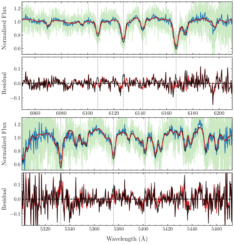
Figure 1: The CFHT spectrum and the best fitting templates. The green spectrum represents the observed data. The blue curves are the rebined spectrum with 10 times of the sampling interval. The red spectrum corresponds to the best-fitting template. The black spectrum is the broadened template using a rotational kernel of $v\sin i=94\,\mathrm{km\,s^{-1}}$ (Lin et al., 2023). The residuals between the rebined spectrum and the templates are shown in lower panels. Grey vertical dotted lines indicate strong stellar absorption lines.

Table 1: The fitting results of CFHT spectrum

Parameter	First scheme	Second scheme
$T_{\mathrm{eff}}$	3919	$4076.8_{-9.7}^{+10.1}$
$\log g$	$4.81_{-0.03}^{+0.04}$	$4.98_{-0.02}^{+0.01}$
$\mathrm{[M/H]}$	$-0.38_{-0.01}^{+0.01}$	$-0.34_{-0.01}^{+0.01}$
$v\sin i$	$120.7_{-0.9}^{+1.0}$	$122.5_{-1.0}^{+1.1}$
$\chi^{2}$	103,203.6	102,916.4
$\chi^{2}_{\mathrm{lin}}$	103,994.7	103,877.4

Note. — The first scheme corresponds to the fitting results with a fixed temperature, while the second scheme represents the fitting outcomes with temperature as a fitting parameter. The final line denotes the chi-squares calculated between the observed data and the templates broadened using $v\sin i_{\mathrm{lin}}=94\,\mathrm{km\,s^{-1}}$ (Lin et al., 2023), with their stellar parameters fixed at the values listed in the respective columns.

The typical SNR of our CFHT spectrum is about 10 (the SNR increases with wavelength in the range we use, reaching an SNR of 18 at the red end), which is relatively modest. A valid concern is that the SNR may affect $v\sin i$ measurement. To investigate this matter, we resample the CFHT spectrum and adjust the sampling interval to be 10 times that of the original, thereby increasing the SNR to 32. The resolution of the resampled spectrum is reduced to 17,000, which remains sufficiently high to preclude any significant broadening effects due to under-sampling. We apply the same method to the resampled spectrum, and the best-fitting $v\sin i$ is consistent with our previous measurements. Hence, our $v\sin i$ measurement is robust against data noises.

4 Discussion

The best-fitting effective temperature in our $v\sin i$ measurement is $T_{\mathrm{eff}}=4076.8_{-9.7}^{+10.1}$ K, slightly larger than the temperature ($T_{\mathrm{eff,lin}}=3919_{-40}^{+31}$ K) reported by Lin et al. (2023). For parameter consistency, we undertake a re-fit of the Spectral Energy Distribution (SED) of J1527 utilizing astroARIADNE (Vines & Jenkins, 2022). Here, we establish a prior for the effective temperature as $T_{\mathrm{eff}}=4076.8\pm 10$ K. The radius yielded by this re-fitting is $R=0.637_{-0.004}^{+0.007}R_{\odot}$, slightly less than the radius ($R_{\mathrm{lin}}=0.685_{-0.010}^{+0.016}\,R_{\odot}$) reported in Lin et al. (2023).

The mass function for a binary system in a circular orbit is defined as follows:

$$f(M_{2})=\frac{M_{2}^{3}\sin^{3}i}{(M_{1}+M_{2})^{2}}=\frac{K_{\mathrm{obs}}^{3}P_{\mathrm{orb}}}{2\pi G},$$ (3)

where $M_{1}$ and $M_{2}$ represent the masses of the visible star and the compact object, respectively; $i$ denotes the inclination angle; $K_{\mathrm{obs}}$ is the semi-amplitude of the observed RV curve, $P_{\mathrm{orb}}$ is the orbital period, and $G$ stands for the gravitational constant. We adopt the mass function of $f(M_{2})=0.131\pm 0.002$ $M_{\odot}$ reported by Lin et al. (2023). For the mass of the visible star, $M_{1}$, we estimate it using the relationship between $K_{s}$-band absolute magnitude and stellar mass provided by Mann et al. (2019). Based on the apparent magnitude of J1527, $\mathrm{Mag}(K_{s})=10.15\pm 0.02$, and its distance, $D=118.1\pm 0.1$ pc, we constrain the mass of the visible star to be $M_{1}=0.63\pm 0.02$ $M_{\odot}$.

According to the estimated mass and radius of the visible star, its filling factor is about 0.92. In this case, the visible star is significantly distorted by the gravitational force of the unseen companion. Consequently, the projected rotational velocity, $v\sin i$, varies with the orbital phase, as discussed in Shahbaz (1998); Jayasinghe et al. (2021); Masuda & Hirano (2021). Given the notable distortion of the visible star, it is inappropriate to use $V_{\mathrm{rot}}=2\pi\,R/P_{\mathrm{orb}}$ (where $P_{\mathrm{orb}}=0.2556698$ days is orbital period) to calculate $V_{\mathrm{rot}}$. Therefore, we use Phoebe (Prša, 2018) to compute the rotational velocity at the spectral observation phase (phase=0.756) as a given inclination angle. Our steps to determine the inclination angle are as follows. First, we start with an arbitrary inclination angle ($75$ degrees) and use Phoebe to compute $V_{\mathrm{rot}}$. Second, we use the calculated $V_{\mathrm{rot}}$ and our $v\sin i$ measurement to obtain a new $i$. Third, we adopt the new $i$ and repeat the first and second steps. This iteration stops when the inclination angle does not change between the first and third steps. We obtain a self-consistent rotational velocity of $V_{\mathrm{rot}}=137.7\pm 2.1\,\mathrm{km\,s^{-1}}$. This value corresponds to an inclination of $i=63\pm 2^{\circ}$, and a mass of the compact object of $M_{2}=0.69\pm 0.02\,M_{\odot}$. The mass of the compact object is much smaller than the result of Lin et al. (2023)

Our spectroscopic observation was conducted only at $\mathrm{phase}=0.756$, corresponding nearly to the maximum value of $v\sin i$. Based on the current fitting parameters, we anticipate the $v\sin i$ measurement to be minimal at phases 0 and 0.5, which is $111.2\,\mathrm{km\,s^{-1}}$. High-resolution spectroscopic observations at other phases could check our measurements and provide a more stringent constraint on the orbital inclination.

The light curves of J1527 show significant variations in its profile during different observation epochs (see figure 6 in Lin et al. 2023). Moreover, the light curve of each observation can not be described well by a pure ellipsoidal variation model. Hence, Lin et al. (2023) has to introduce significant surface spot activity on the visible star to fit the observed light curves. As pointed out by Luger et al. (2021) and Rowan et al. (2023), the inclination angle cannot be well determined if the tidally distorted star has star spots. In this case, we speculate that the inclination angle cannot be robustly determined by analyzing the light curves.

The $\mathrm{H\alpha}$ emission line of J1527 exhibits features of multiple components (see Figure 4 in Lin et al. 2023). Part of the emission line is likely to be caused by the stellar activity of the visible star, while the other part may be from the accretion process of the companion. Similar observational characteristics have been reported in a series of previous works (e.g., Tappert et al., 2007, 2011; Parsons et al., 2012). These objects are thought to be detached binaries that consist of a WD and a K/M companion star almost filling its Roche lobe, thereby qualifying them as pre-cataclysmic variables (pre-CVs). The WDs in these pre-CVs accrete material from the wind of the K/M companion star, leading to additional emission features. Lin et al. (2023) argue that if the unseen object is a WD, its temperature limit derived from the SED fitting corresponds to a lower accretion rate, which is inconsistent with the observed $\mathrm{H\alpha}$ emission line, and the system should exhibit dwarf nova phenomena. However, the temperature of the WDs in these binaries can be notably low; for instance, Parsons et al. (2012) reported a binary, SDSS J013851.54-001621.6, with an $\mathrm{H\alpha}$ emission line from WD and a WD temperature of about $3600$ K. J1527 might also be a pre-CV system.

5 Conclusions

We have performed a spectroscopic observation of an NS candidate reported by Lin et al. (2023), J1527, using the CFHT telescope. The high resolution of the CFHT spectrum enables us to make a reliable $v\sin i$ measurement. Through a concurrent fitting of stellar parameters and $v\sin i$, we have determined that the projected rotational velocity of J1527 is $v\sin i=122.5_{-1.0}^{+1.1}\,\mathrm{km\,s^{-1}}$, accompanied by an estimated orbital inclination of $63\pm 2^{\circ}$. This result deviates significantly from the inclination estimation of about $45^{\circ}$ presented in Lin et al. (2023). Considering that the complex optical variation characteristics of J1527 make it problematic to constrain the inclination angle, the $v\sin i$ measurements based on CFHT’s high-resolution spectrum is more reliable. Based on our inferred orbital inclination, we have constrained the mass of the compact object in this system to be $M_{2}=0.69\pm 0.02\,M_{\odot}$, falling within the typical mass range of WD.

References

- Astropy Collaboration et al. (2013) Astropy Collaboration, Robitaille, T. P., Tollerud, E. J., et al. 2013, A&A, 558, A33, doi: 10.1051/0004-6361/201322068
- Astropy Collaboration et al. (2018) Astropy Collaboration, Price-Whelan, A. M., Sipőcz, B. M., et al. 2018, AJ, 156, 123, doi: 10.3847/1538-3881/aabc4f
- Berghöfer & Breitschwerdt (2002) Berghöfer, T. W., & Breitschwerdt, D. 2002, A&A, 390, 299, doi: 10.1051/0004-6361:20020627
- Camenzind (2007) Camenzind, M. 2007, Compact objects in astrophysics : white dwarfs, neutron stars, and black holes, doi: 10.1007/978-3-540-49912-1
- Claret & Bloemen (2011) Claret, A., & Bloemen, S. 2011, A&A, 529, A75, doi: 10.1051/0004-6361/201116451
- Clough et al. (1992) Clough, S. A., Iacono, M. J., & Moncet, J.-L. 1992, J. Geophys. Res., 97, 15,761, doi: 10.1029/92JD01419
- Clough et al. (2005) Clough, S. A., Shephard, M. W., Mlawer, E. J., et al. 2005, J. Quant. Spec. Radiat. Transf., 91, 233, doi: 10.1016/j.jqsrt.2004.05.058
- El-Badry et al. (2023) El-Badry, K., Rix, H.-W., Cendes, Y., et al. 2023, MNRAS, 521, 4323, doi: 10.1093/mnras/stad799
- Foreman-Mackey et al. (2013) Foreman-Mackey, D., Hogg, D. W., Lang, D., & Goodman, J. 2013, PASP, 125, 306, doi: 10.1086/670067
- Gray (2005) Gray, D. F. 2005, The Observation and Analysis of Stellar Photospheres
- Gullikson et al. (2014) Gullikson, K., Dodson-Robinson, S., & Kraus, A. 2014, AJ, 148, 53, doi: 10.1088/0004-6256/148/3/53
- Gustafsson et al. (2008) Gustafsson, B., Edvardsson, B., Eriksson, K., et al. 2008, A&A, 486, 951, doi: 10.1051/0004-6361:200809724
- Heiter et al. (2021) Heiter, U., Lind, K., Bergemann, M., et al. 2021, A&A, 645, A106, doi: 10.1051/0004-6361/201936291
- Jayasinghe et al. (2021) Jayasinghe, T., Stanek, K. Z., Thompson, T. A., et al. 2021, MNRAS, 504, 2577, doi: 10.1093/mnras/stab907
- Koll et al. (2019) Koll, D., Korschinek, G., Faestermann, T., et al. 2019, Phys. Rev. Lett., 123, 072701, doi: 10.1103/PhysRevLett.123.072701
- Lin et al. (2023) Lin, J., Li, C., Wang, W., et al. 2023, ApJ, 944, L4, doi: 10.3847/2041-8213/acb54b
- Luger et al. (2021) Luger, R., Foreman-Mackey, D., Hedges, C., & Hogg, D. W. 2021, AJ, 162, 123, doi: 10.3847/1538-3881/abfdb8
- Mann et al. (2019) Mann, A. W., Dupuy, T., Kraus, A. L., et al. 2019, ApJ, 871, 63, doi: 10.3847/1538-4357/aaf3bc
- Masuda & Hirano (2021) Masuda, K., & Hirano, T. 2021, ApJ, 910, L17, doi: 10.3847/2041-8213/abecdc
- Mazeh et al. (2022) Mazeh, T., Faigler, S., Bashi, D., et al. 2022, MNRAS, 517, 4005, doi: 10.1093/mnras/stac2853
- Morton (2015) Morton, T. D. 2015, isochrones: Stellar model grid package, Astrophysics Source Code Library, record ascl:1503.010. http://ascl.net/1503.010
- Mu et al. (2022) Mu, H.-J., Gu, W.-M., Yi, T., et al. 2022, Science China Physics, Mechanics, and Astronomy, 65, 229711, doi: 10.1007/s11433-021-1809-8
- Özel & Freire (2016) Özel, F., & Freire, P. 2016, ARA&A, 54, 401, doi: 10.1146/annurev-astro-081915-023322
- Parsons et al. (2012) Parsons, S. G., Gänsicke, B. T., Marsh, T. R., et al. 2012, MNRAS, 426, 1950, doi: 10.1111/j.1365-2966.2012.21773.x
- Plez (2012) Plez, B. 2012, Turbospectrum: Code for spectral synthesis, Astrophysics Source Code Library, record ascl:1205.004. http://ascl.net/1205.004
- Prša (2018) Prša, A. 2018, Modeling and Analysis of Eclipsing Binary Stars; The theory and design principles of PHOEBE, doi: 10.1088/978-0-7503-1287-5
- Rowan et al. (2023) Rowan, D. M., Jayasinghe, T., Tucker, M. A., et al. 2023, arXiv e-prints, arXiv:2307.11146, doi: 10.48550/arXiv.2307.11146
- Ryabchikova et al. (2015) Ryabchikova, T., Piskunov, N., Kurucz, R. L., et al. 2015, Phys. Scr, 90, 054005, doi: 10.1088/0031-8949/90/5/054005
- Schulreich et al. (2017) Schulreich, M. M., Breitschwerdt, D., Feige, J., & Dettbarn, C. 2017, A&A, 604, A81, doi: 10.1051/0004-6361/201629837
- Shahbaz (1998) Shahbaz, T. 1998, MNRAS, 298, 153, doi: 10.1046/j.1365-8711.1998.01618.x
- Smith & Cox (2001) Smith, R. K., & Cox, D. P. 2001, ApJS, 134, 283, doi: 10.1086/320850
- Stoica & Selen (2004) Stoica, P., & Selen, Y. 2004, IEEE Signal Processing Magazine, 21, 36, doi: 10.1109/MSP.2004.1311138
- Tappert et al. (2011) Tappert, C., Gänsicke, B. T., Rebassa-Mansergas, A., Schmidtobreick, L., & Schreiber, M. R. 2011, A&A, 531, A113, doi: 10.1051/0004-6361/201116833
- Tappert et al. (2007) Tappert, C., Gänsicke, B. T., Schmidtobreick, L., et al. 2007, A&A, 474, 205, doi: 10.1051/0004-6361:20077316
- Vines & Jenkins (2022) Vines, J. I., & Jenkins, J. S. 2022, MNRAS, 513, 2719, doi: 10.1093/mnras/stac956
- Virtanen et al. (2020) Virtanen, P., Gommers, R., Oliphant, T. E., et al. 2020, Nature Methods, 17, 261, doi: 10.1038/s41592-019-0686-2
- Wallner et al. (2021) Wallner, A., Froehlich, M. B., Hotchkis, M. A. C., et al. 2021, Science, 372, 742, doi: 10.1126/science.aax3972
- Yi et al. (2019) Yi, T., Sun, M., & Gu, W.-M. 2019, ApJ, 886, 97, doi: 10.3847/1538-4357/ab4a75
- Yuan et al. (2022) Yuan, H., Wang, S., Bai, Z., et al. 2022, ApJ, 940, 165, doi: 10.3847/1538-4357/ac9c62
- Zheng et al. (2022) Zheng, L.-L., Sun, M., Gu, W.-M., et al. 2022, arXiv e-prints, arXiv:2210.04685, doi: 10.48550/arXiv.2210.04685