Treated	Treated	Non-treated	Non-treated
	Non-Swiss	Swiss	Non-Swiss	Swiss
Variable	Mean	Mean	Mean	Mean
Age	35.62	38.08	36.37	36.50
Female	0.40	0.47	0.41	0.46
Married	0.67	0.36	0.70	0.35
Mother tongue not Swiss language	0.65	0.10	0.66	0.10
Past annual income	41704	47899	38226	43865
Previous job: manager	0.05	0.09	0.04	0.09
Previous job: primary sector	0.07	0.05	0.13	0.08
Previous job: secondary sector	0.18	0.15	0.13	0.13
Previous job: tertiary sector	0.54	0.67	0.48	0.64
Previous job: missing sector	0.21	0.13	0.26	0.15
Previous job: self-employed	0.00	0.00	0.01	0.01
Previous job: skilled worker	0.47	0.72	0.45	0.70
Previous job: unskilled worker	0.47	0.16	0.48	0.17
Qualification: some degree	0.35	0.73	0.32	0.73
Qualification: semiskilled	0.18	0.13	0.21	0.13
Qualification: unskilled	0.40	0.13	0.40	0.12
Qualification: skilled without degree	0.07	0.02	0.08	0.03
No of unemployment spells last 2 years	0.54	0.35	0.78	0.50

Number of observations 4438 8607 30417 47877

• Note: This table shows the mean of some covariates included in the analysis. Column (1) and (2) show it for treated individuals, column (3) and (4) for non-treated individuals. Column (1) and (3) show it for non-Swiss individuals, column (2) and (4) for Swiss individuals.

5.3 Empirical results

Table 3 shows the effects considered in the analysis. These effects include the $\Delta$GATE, a $\Delta$BGATE with already balanced covariates, such as age and gender, a $\Delta$BGATE with additionally adding marital status, an extended $\Delta$BGATE balancing additionally unbalanced covariates like past annual income, previous job variables, and qualification variables. Then, we further add the mother tongue variable, and finally, the analysis considers a $\Delta$BGATE that balances all covariates included in the study.

Table 3: Empirical analysis: Effects of interest

max width= Effect Variables used for balancing in the $\Delta$BGATE $\theta^{\Delta G}$ none $\theta_{1}^{\Delta B}$ age, female $\theta_{2}^{\Delta B}$ + married $\theta_{3}^{\Delta B}$ + past income and unemployment spells, previous job variables, qualification variables $\theta_{4}^{\Delta B}$ + mother tongue not Swiss language $\theta_{5}^{\Delta B}$ all covariates included in the analysis

• Note: This table shows the effects of interest for the empirical analysis.

As a reference point, the treatment effect for Swiss individuals in the lock-in period is $\tau_{swiss}=-0.907$ ($0.015$) and for foreigners $\tau_{foreigner}=-0.706$ ($0.017$). Hence, it seems the programme works better for foreigners. However, as pointed out above, the interpretation is not straightforward because the two groups have unbalanced covariates. Table 5.3 depicts the results for the different effects. $\theta^{\Delta G}$ shows that the difference between Swiss and non-Swiss is significant. After balancing already balanced socio-demographic characteristics like age and gender, the coefficient remains relatively stable. When marital status is further balanced, there is a notable reduction in the coefficient. Subsequently, balancing the labour market history, including covariates like past income and previous job details, further reduces the observed difference. As anticipated, additionally, balancing mother tongue results in a minimal difference between Swiss and non-Swiss individuals of only 0.05. Balancing all covariates included in the analysis reduces the difference to zero. Hence, it becomes evident that marital status, mother tongue disparities and differences in the labour market history significantly contribute to the variance in treatment effects between Swiss and non-Swiss individuals.

These results show that researchers must carefully interpret group average treatment effects. For example, the different effect for foreigners compared to Swiss individuals is likely not caused by nationality but probably comes from different characteristics of foreigners compared to Swiss individuals.

Table 4: Empirical analysis: Differences of $\Delta$BGATEs for Swiss nationals versus foreigners.

max width=

• Note: This table shows the results of the empirical example ($N=91,339$).

6 Causal moderation

6.1 Effect of interest

Suppose we want to interpret the difference in treatment effects between two groups causally. Then a different but closely related parameter is needed, namely the causal balanced group average treatment effect ($\Delta$CBGATE).

To define the $\Delta$CBGATE we first introduce potential outcomes that additionally depend on the moderator $Z$, i.e. $(Y_{0,0},Y_{1,0},Y_{0,1},Y_{1,1})$.

The new parameter of interest is defined as follows:

$$\theta^{\Delta C}=\mathrm{E}\left[\left(Y_{1,1}-Y_{0,1}\right)-\left(Y_{1,0}-Y_{0,0}\right)\right]=\int_{X}(\tau(X,1)-\tau(X,0))f_{X}(x)dx$$

The $\Delta$CBGATE represents the difference between the two groups, balancing the distribution of all the other covariates. To identify this effect, we have to introduce new identifying assumptions. The conditions to obtain a causally interpretable $\Delta$CBGATE may be challenging in many applications.

6.2 Identifiying assumptions

In addition to the usual identifying assumptions stated in Section LABEL:2_identifying_assumptions, we apply the unconfoundedness setting to the moderator variable to be able to interpret the $\Delta$CBGATE causally. Hence, the following assumptions have to be changed or added in comparison to the assumptions for the $\Delta$BGATE in Section LABEL:2_identifying_assumptions.

Assumption 10.

(CIA for moderator)

$$(Y_{1,1},Y_{0,1},Y_{1,0},Y_{0,0})\perp Z|X=x\quad\forall x\in X$$

The CIA assumption for a moderator variable states that the potential outcomes are independent of the effect moderator $(Z)$, conditionally on confounding variables.

Assumption 11.

(CS for moderator)

$$0<P(Z=z|X=x)<1,\quad\forall z\in\{0,1\}$$

For any given values of $X$ it must be possible to observe each moderator variable status $Z\in\{0,1\}$.

Assumption 12.

(Exogenity of confounders and moderator)

$$Z_{0} =Z_{1}$$

$$X_{0,0} =X_{0,1}$$

where $Z_{d}$ are potential moderators that depend on the treatment and $X_{d,z}$ are potential confounders that depend on the treatment and the moderator.

New about the exogeneity assumption is that the moderator must not influence the confounders in a way related to the outcome variable. This assumption is non-standard and might be hard to fulfil in some applications. It often happens that a moderator variable such as gender influences other covariates, violating this assumption.

Assumption 13.

(Stable Unit Treatment Value Assumption (SUTVA))

$$Y=\sum_{z=0}^{1}\sum_{d=0}^{1}I(d,z)Y_{d,z}$$

SUTVA now additionally requires that there are no unrepresented moderators in the population of interest (everyone is assigned to a moderation group) and that there are no relevant interactions between groups, meaning that the assignment of individual $i$ to one group does not influence the outcome of individual $j$.

Lemma 2.

Under Assumptions 10 to 13 the parameter $\theta^{\Delta C}=\mathrm{E}\left[\left(Y_{1,1}-Y_{0,1}\right)-\left(Y_{1,0}-Y_{0,0}\right)\right]$ is identified as $\mathrm{E}\left[\mu_{1,1}(X)-\mu_{0,1}(X)-\mu_{1,0}(X)+\mu_{0,0}(X)\right]$ with $\mu_{d,z}(X)=\mathrm{E}[Y|D=d,Z=z,X]$.

For the proof of Lemma 2, see Appendix A.3.1. The $\Delta CBGATE$ is the same effect as a fully balanced $\Delta BGATE$ for which Assumptions 10 to 13 hold.

6.3 Estimation and Inference

To obtain an efficient and flexible estimator, we use DML. As shown in detail in Appendix A.3.4, the Neyman-orthogonal score based on the efficient influence function for the $\Delta$CBGATE is given by:

$$\phi^{\Delta C}(X;\hat{\theta}^{\Delta C},\hat{\eta}) =\hat{\mu}_{1,1}(X)-\hat{\mu}_{0,1}(X)-\hat{\mu}_{1,0}(X)+\hat{\mu}_{0,0}(X)$$

$$+\frac{DZ(Y-\hat{\mu}_{1,1}(X))}{\hat{\omega}_{1,1}(X)}-\frac{(1-D)Z(Y-\hat{\mu}_{0,1}(X))}{\hat{\omega}_{0,1}(X)}$$

$$-\frac{D(1-Z)(Y-\hat{\mu}_{1,0}(X))}{\hat{\omega}_{1,0}(X)}+\frac{(1-D)(1-Z)(Y-\hat{\mu}_{0,0}(X))}{\hat{\omega}_{0,0}(X)}-\hat{\theta}^{\Delta C}$$

with $\hat{\omega}_{d,z}(X)=P(D=d,Z=z|X)$ and $\hat{\mu}_{d,z}(X)=\mathrm{E}[Y|D=d,Z=z,X]$ and the nuisance parameters $\hat{\eta}=(\hat{\mu}_{d,z}(X),\hat{\omega}_{d,z}(X))$. Using this double robust moment condition, the $\Delta$CBGATE is estimated at a convergence rate of $\sqrt{N}$, even if the nuisance parameters are estimated with slower rates (Smucler, Rotnitzky  Robins, 2019). However, they must converge such that the product of the convergence rates of the outcome regression score and the propensity score estimator is faster than or equal to $\sqrt{N}$. Many common machine learning algorithms are known to converge at a rate faster or equal to $N^{1/4}$ but slower than $\sqrt{N}$ (Chernozhukov et al., 2018). Furthermore, as before, we use cross-fitting with K-folds. An estimator based on these elements is $\sqrt{N}$-consistent, asymptotically normal, and asymptotically efficient (Kennedy, 2022).

Hence, the variance of $\hat{\theta}^{\Delta C}$ can be defined as

$$\operatorname{Var}(\hat{\theta}^{\Delta C}) =\operatorname{Var}(\phi^{\Delta C}(X;\hat{\theta}^{\Delta C},\hat{\eta}))$$

$$=\mathrm{E}[\phi^{\Delta C}(X;\hat{\theta}^{\Delta C},\hat{\eta})^{2}]-\underbrace{\mathrm{E}[\phi^{\Delta C}(X;\hat{\theta}^{\Delta C},\hat{\eta})]^{2}}_{=0}$$

$$=\mathrm{E}[\phi^{\Delta C}(X;\hat{\theta}^{\Delta C},\hat{\eta})^{2}]$$

and can be estimated as follows:

$$\widehat{Var(\theta^{\Delta C})}=\frac{1}{N}\sum_{k=1}^{K}\sum_{i\in S_{k}}[\phi^{\Delta C}(X;\hat{\theta}^{\Delta C},\hat{\eta})]^{2}$$

Concerning the practical implementation, any machine learner with the required convergence rates can be used to estimate the nuisance parameters. Note that since $P(D=d,Z=z|X)$ can be rewritten as $P(D=d|X=x,Z)\cdot P(Z=z|X)$, there are two basic versions of the estimator. One version is based on directly estimating $P(D=d,Z=z|X)$. In contrast, the second version is based on estimating $P(D=d|X,Z)$ and $P(Z=z|X)$ separately in the full sample and subsequently obtaining the estimate of $P(D=d,Z=z|X)$ as the product of these two estimates. For the proof that the second version of the estimator is also $\sqrt{N}$-consistent and asymptotically normal, see Appendix A.3.5. Same as for the $\Delta$BGATE, we normalise the weights (e.g.,$\frac{DZ}{\omega_{1,1}(X)}$) to ensure that the weighted residuals do not have much more weight than the outcome regression (see Algorithm 2). The proposed algorithm is summarised in Appendix B. A small simulation study in Appendix C.3 shows the finite sample properties of the estimator and its difference to the $\Delta$GATE.

7 Conclusion

This paper presents a novel approach for analysing and interpreting treatment heterogeneity in an unconfoundedness setting. We introduce a parameter called $\Delta$BGATE for measuring the difference in treatment effects between different groups while accounting for variations in covariates. Moreover, this paper proposes an estimator based on DML for discrete treatments and discrete moderators, demonstrating its consistency and asymptotic normality under standard conditions. A simulation study shows that the estimation strategy seems to have good finite sample properties and that estimating a $\Delta$GATE may lead to substantially different results than estimating a $\Delta$BGATE if the covariates are not balanced. An empirical example illustrates the proposed estimand and underlines that seeming causal heterogeneity may be caused by an underlying different distribution of other covariates. Moreover, by incorporating additional assumptions, the paper introduces the $\Delta$CBGATE, enabling a causal interpretation of the differences in treatment effects. The proposed new parameters allow a more informative interpretation of causal heterogeneity and thus a better understanding of the differential impact of decisions. Future research could extend the estimation approach to continuous treatments and moderators. Furthermore, this paper shows identification in an unconfoundedness setting. Extending it to an instrumental variable setting for the treatment, the moderator, or both, would be interesting. More extensive simulation studies will lead to a more comprehensive picture of the finite sample properties of the proposed estimators.

Appendix A Appendix: Theory

A.1 Notation

The model considered here is more general than in the main body of the paper; let the treatment be $D\in\{0,1,\dots,m\}$ ($0=$ no treatment) and the moderator be $Z\in\{0,1,2,\dots,v\}$ variables which are discrete. To identify the effects, we rely on the usual potential outcomes by treatment $(Y_{0},Y_{1},\dots,Y_{m})$. Furthermore, we have an indicator function $I(d)=\mathds{1}(D=d)$, which takes the value one if $D=d$ and zero otherwise, and an indicator function $I(z)=\mathds{1}(Z=z)$ which takes the value one if $Z=z$ and zero otherwise. The analysis examines pairwise comparisons between two treatments, denoted as $m$ and $l$, and two moderator groups represented as $u$ and $v$.

A.2 $\Delta$BGATE

A.2.1 Indentification based on the outcome regression

In this subsection, the identification of the BGATE with Assumptions LABEL:assumption_CIA to LABEL:assumption_SUTVA stated in Section LABEL:2_identifying_assumptions is shown. Due to the linearity in expectations assumption, the identification for the $\Delta$BGATE directly follows. Please recall that $\mu_{d}(Z,X)=\mathrm{E}[Y|D=d,Z,X]$.

$$\mathrm{E}\Bigl{[}\mathrm{E}[ Y_{l}-Y_{m}\mid Z=z,W]\Bigr{]}$$

$$=\mathrm{E}\Bigl{[} \mathrm{E}\left[\mathrm{E}\left[Y_{l}-Y_{m}\mid X,Z\right]\mid Z=z,W\right]\Bigr{]}$$

$$=\mathrm{E}\Bigl{[} \mathrm{E}\left[\mathrm{E}[Y_{l}\mid X,Z]-\mathrm{E}[Y_{m}\mid X,Z]\mid Z=z,W\right]\Bigr{]}$$

$$=\mathrm{E}\Bigl{[} \mathrm{E}\left[\mathrm{E}[Y_{l}\mid D=l,X,Z]-\mathrm{E}[Y_{m}\mid D=m,X,Z]\mid Z=z,W\right]\Bigr{]}$$

$$=\mathrm{E}\Bigl{[} \mathrm{E}\left[\mathrm{E}[Y\mid D=l,X,Z]-\mathrm{E}[Y\mid D=m,X,Z]\mid Z=z,W\right]\Bigr{]}$$

$$=\mathrm{E}\Bigl{[} \mathrm{E}\left[\mu_{l}(Z,X)-\mu_{m}(Z,X)\mid Z=z,W\right]\Bigr{]}$$

The first equality is derived from the law of iterated expectations, while the second equality follows from the linearity in expectations. The third equality is based on Assumption LABEL:assumption_CIA, and the fourth is derived from the law of total expectation.

A.2.2 Identification based on the doubly robust score

The BGATE can also be identified with the doubly robust score function (see Section LABEL:2_estimation in the main body of the text). Please recall that $\pi_{d}(Z,X)=P(D=d|Z,X)$ and $\lambda_{z}(X)=P(Z=d|W)$. For better readability $\mu_{l}(Z,X)-\mu_{m}(Z,X)+\frac{I(l)(Y-\mu_{l}(Z,X))}{\pi_{l}(Z,X)}-\frac{I(m)(Y-\mu_{m}(Z,X))}{\pi_{m}(Z,X)}$ is denoted as $\delta_{l,m}(Z,X)$.

$$\mathrm{E}[ \mathrm{E}[Y_{l}-Y_{m}|Z=z,W]]$$

$$=\mathrm{E}\Biggl{[}\mathrm{E}\Biggl{[}\mathrm{E}\left[\delta_{l,m}(Z,X)\mid Z=z,W\right]+\frac{I(z)(\delta_{l,m}(Z,X)-\mathrm{E}\left[\delta_{l,m}(Z,X)\mid Z=z,W\right])}{\lambda_{z}(W)}\bigg{|}W\Biggr{]}\Biggr{]}$$

$$=\mathrm{E}\Biggl{[}\mathrm{E}\left[\delta_{l,m}(Z,X)\mid Z=z,W\right]+\mathrm{E}\Biggl{[}\frac{I(z)(\delta_{l,m}(Z,X)-\mathrm{E}\left[\delta_{l,m}(Z,X)\mid Z=z,W\right])}{\lambda_{z}(W)}\bigg{|}W\Biggr{]}\Biggr{]}$$

$$=\mathrm{E}\Biggl{[}\mathrm{E}\left[\delta_{l,m}(Z,X)\mid Z=z,W\right]+\mathrm{E}\Biggl{[}\frac{I(z)(\delta_{l,m}(Z,X)-\mathrm{E}\left[\delta_{l,m}(Z,X)\mid Z=z,W\right])}{\lambda_{z}(W)}\bigg{|}W,Z=z\Biggr{]}\lambda_{z}(W)\Biggr{]}$$

$$=\mathrm{E}\biggl{[}\mathrm{E}\left[\delta_{l,m}(Z,X)\mid Z=z,W\right]+\mathrm{E}[\delta_{l,m}(Z,X)-\mathrm{E}\left[\delta_{l,m}(Z,X)\mid Z=z,W\right]|Z=z,W]\biggr{]}$$

$$=\mathrm{E}[\mathrm{E}[\delta_{l,m}(Z,X)|Z=z,W]]$$

The first equality follows from the law of iterated expectations, and the third from the law of total expectation. Hence, the BGATE can be identified if the nuisance functions are correctly specified. Due to the double robustness property, the BGATE is also identified if only the outcome regression or the propensity score is correctly specified.

Correctly specified propensity score $\lambda_{z}(W)$ and wrongly specified outcome regression function $\bar{\mathrm{E}}\left[\delta_{l,m}(Z,X)\mid Z=z,W\right]$:

$$\mathrm{E}[ \mathrm{E}[Y_{l}-Y_{m}|Z=z,W]]$$

$$=\mathrm{E}\Biggl{[}\mathrm{E}\Biggl{[}\bar{\mathrm{E}}\left[\delta_{l,m}(Z,X)\mid Z=z,W\right]+\frac{I(z)(\delta_{l,m}(Z,X)-\bar{\mathrm{E}}\left[\delta_{l,m}(Z,X)\mid Z=z,W\right])}{\lambda_{z}(W)}\bigg{|}W\Biggr{]}\Biggr{]}$$

$$=\mathrm{E}\Biggl{[}\bar{\mathrm{E}}\left[\delta_{l,m}(Z,X)\mid Z=z,W\right]+\mathrm{E}\Biggl{[}\frac{I(z)(\delta_{l,m}(Z,X)-\bar{\mathrm{E}}\left[\delta_{l,m}(Z,X)\mid Z=z,W\right])}{\lambda_{z}(W)}\bigg{|}W\Biggr{]}\Biggr{]}$$

$$=\mathrm{E}\Biggl{[}\bar{\mathrm{E}}\left[\delta_{l,m}(Z,X)\mid Z=z,W\right]+\mathrm{E}\Biggl{[}\frac{I(z)(\delta_{l,m}(Z,X)-\bar{\mathrm{E}}\left[\delta_{l,m}(Z,X)\mid Z=z,W\right])}{\lambda_{z}(W)}\bigg{|}W,Z=z\Biggr{]}\lambda_{z}(W)\Biggr{]}$$

$$=\mathrm{E}\biggl{[}\bar{\mathrm{E}}\left[\delta_{l,m}(Z,X)\mid Z=z,W\right]+\mathrm{E}[\delta_{l,m}(Z,X)-\bar{\mathrm{E}}\left[\delta_{l,m}(Z,X)\mid Z=z,W\right]|Z=z,W]\biggr{]}$$

$$=\mathrm{E}\biggl{[}\bar{\mathrm{E}}\left[\delta_{l,m}(Z,X)\mid Z=z,W\right]+\mathrm{E}[\delta_{l,m}(Z,X)|Z=z,W]-\bar{\mathrm{E}}\left[\delta_{l,m}(Z,X)\mid Z=z,W\right]\biggr{]}$$

$$=\mathrm{E}[\mathrm{E}[\delta_{l,m}(Z,X)|Z=z,W]]$$

Correctly specified outcome regression $\mathrm{E}\left[\delta_{l,m}(Z,X)\mid Z=z,W\right]$ and wrongly specified propensity score $\bar{\lambda}_{z}(W)$:

$$\mathrm{E}[ \mathrm{E}[Y_{l}-Y_{m}|Z=z,W]]$$

$$=\mathrm{E}\Biggl{[}\mathrm{E}\Biggl{[}\mathrm{E}\left[\delta_{l,m}(Z,X)\mid Z=z,W\right]+\frac{I(z)(\delta_{l,m}(Z,X)-\mathrm{E}\left[\delta_{l,m}(Z,X)\mid Z=z,W\right])}{\bar{\lambda}_{z}(W)}\bigg{|}W\Biggr{]}\Biggr{]}$$

$$=\mathrm{E}\Biggl{[}\mathrm{E}\left[\delta_{l,m}(Z,X)\mid Z=z,W\right]+\mathrm{E}\Biggl{[}\frac{I(z)(\delta_{l,m}(Z,X)-\mathrm{E}\left[\delta_{l,m}(Z,X)\mid Z=z,W\right])}{\bar{\lambda}_{z}(W)}\bigg{|}W\Biggr{]}\Biggr{]}$$

$$=\mathrm{E}\Biggl{[}\mathrm{E}\left[\delta_{l,m}(Z,X)\mid Z=z,W\right]+\mathrm{E}\Biggl{[}\frac{I(z)(\delta_{l,m}(Z,X)-\mathrm{E}\left[\delta_{l,m}(Z,X)\mid Z=z,W\right])}{\bar{\lambda}_{z}(W)}\bigg{|}W,Z=z\Biggr{]}\lambda_{z}(W)\Biggr{]}$$

$$=\mathrm{E}\Biggl{[}\mathrm{E}\left[\delta_{l,m}(Z,X)\mid Z=z,W\right]+\frac{\lambda_{z}(W)}{\bar{\lambda}_{z}(W)}\left(\mathrm{E}\left[\delta_{l,m}(Z,X)\mid|W,Z=z\right]-\mathrm{E}\left[\delta_{l,m}(Z,X)\mid W,Z=z\right]\right)\Biggr{]}$$

$$=\mathrm{E}[\mathrm{E}[\delta_{l,m}(Z,X)|Z=z,W]]$$

Hence, the BGATE is identified if the outcome regression or the propensity score is correctly specified.

A.2.3 Asymptotic properties

The following proof is for $\theta_{l,m,u,v}^{B}$. However, due to the linearity in expectations, it directly follows that the proof is also valid for $\theta_{l,m,u,v}^{\Delta B}$. In a first step, let us define the following terms for easier readability:

$$\pi_{d}(Z,X) =P(D=d|Z,X)$$

$$\mu_{d}(Z,X) =\mathrm{E}[Y|D=d,Z,X]$$

$$\delta_{l,m}(X,Z) =\mu_{l}(Z,X)-\mu_{m}(Z,X)+\frac{I(l)(Y-\mu_{l}(Z,X))}{\pi_{l}(Z,X)}-\frac{I(m)(Y-\mu_{m}(Z,X))}{\pi_{m}(Z,X)}$$

$$\lambda_{z}(W) =P(Z=z|W)$$

$$\tau_{l,m,z}(W) =\mathrm{E}[\delta_{l,m}(X,Z)|Z=z,W]+\frac{I(z)(\delta_{l,m}(Z,X)-\mathrm{E}[\delta_{l,m}(X,Z)|Z=z,W])}{\lambda_{z}(W)}$$

$$\theta_{l,m,z}^{B} =\mathrm{E}[\tau_{l,m,z}(\delta_{l,m}(X,Z),W)]$$

$$\hat{\mathrm{E}}[f(X)] =\frac{1}{N}\sum_{i=1}^{N}f(x_{i})$$

The goal is to show that

$$\sqrt{N}(\hat{\theta}_{l,m,z}^{B}-\theta_{l,m,z}^{B\star})\xrightarrow{p}N(0,V^{\star})$$

$$V^{\star} =\mathrm{E}\left[\left(\tau_{l,m,z}(\delta_{l,m}(X,Z),W)-\theta_{l,m,z}^{B\star}\right)^{2}\right]$$

with $\theta_{l,m,z}^{B\star}$ being an oracle estimator of $\theta_{l,m,z}^{B}$ if all nuisance functions would be known. Then $\theta_{l,m,z}^{B\star}$ is an i.i.d. average, hence:

$$\sqrt{N}(\theta_{l,m,z}^{B\star}-\theta_{l,m,z}^{B}) \xrightarrow{p}N(0,V^{\star})$$

$$V^{\star} =\mathrm{E}\left[\left(\tau_{l,m,z}(\delta_{l,m}(X,Z),W)-\theta_{l,m,z}^{B\star}\right)^{2}\right]$$

Theorem 2.

Let $\mathcal{I}_{1}$ and $\mathcal{I}_{2}$ be two independent samples such that $|\mathcal{I}_{1}|=|\mathcal{I}_{1}|=\frac{N}{2}$. Furthermore, let $\mathcal{I}_{11}$, $\mathcal{I}_{12}$, $\mathcal{I}_{21}$ and $\mathcal{I}_{22}$ be four samples such that $|\mathcal{I}_{11}|=|\mathcal{I}_{12}|=|\mathcal{I}_{21}|=|\mathcal{I}_{22}|=\frac{|\mathcal{I}_{1}|}{2}=\frac{|\mathcal{I}_{2}|}{2}=\frac{N}{4}$ The second split is independent conditional on the first split. Define the estimator as follows:

$$\hat{\theta}_{l,m,z}^{B} =\frac{|\mathcal{I}_{11}|}{N}\hat{\theta}^{B,\mathcal{I}_{11}}_{l,m,z}+\frac{|\mathcal{I}_{12}|}{N}\hat{\theta}^{B,\mathcal{I}_{12}}_{l,m,z}+\frac{|\mathcal{I}_{21}|}{N}\hat{\theta}^{B,\mathcal{I}_{21}}_{l,m,z}+\frac{|\mathcal{I}_{22}|}{N}\hat{\theta}^{B,\mathcal{I}_{22}}_{l,m,z}$$

$$\hat{\theta}_{l,m,z}^{B,\mathcal{I}_{11}} =\frac{1}{|\mathcal{I}_{11}|}\sum_{\mathcal{I}_{11}}\hat{\tau}_{l,m,z}^{\mathcal{I}_{12}}(\hat{\delta}_{l,m}^{\mathcal{I}_{2}}(X,Z),W)$$

$$\hat{\theta}_{l,m,z}^{B,\mathcal{I}_{12}} =\frac{1}{|\mathcal{I}_{12}|}\sum_{\mathcal{I}_{12}}\hat{\tau}_{l,m,z}^{\mathcal{I}_{11}}(\hat{\delta}_{l,m}^{\mathcal{I}_{2}}(X,Z),W)$$

$$\hat{\theta}_{l,m,z}^{B,\mathcal{I}_{21}} =\frac{1}{|\mathcal{I}_{21}|}\sum_{\mathcal{I}_{21}}\hat{\tau}_{l,m,z}^{\mathcal{I}_{22}}(\hat{\delta}_{l,m}^{\mathcal{I}_{1}}(X,Z),W)$$

$$\hat{\theta}_{l,m,z}^{B,\mathcal{I}_{22}} =\frac{1}{|\mathcal{I}_{22}|}\sum_{\mathcal{I}_{22}}\hat{\tau}_{l,m,z}^{\mathcal{I}_{21}}(\hat{\delta}_{l,m}^{\mathcal{I}_{1}}(X,Z),W)$$

Then, if Assumptions 5 to 8 hold, it follows that

$$\sqrt{N}(\hat{\theta}_{l,m,z}^{B}-\theta_{l,m,z}^{B})\xrightarrow{d}N(0,V^{\star})$$

with

$$V^{\star}=\mathrm{E}\left[\left(\tau_{l,m,z}(\delta_{l,m}(X,Z),W_{i})-\theta_{l,m,z}^{B\star}\right)^{2}\right]$$

Proof.

$$\sqrt{N}(\hat{\theta}_{l,m,z}^{B} -\theta_{l,m,z}^{B})$$

$$=\sqrt{N}(\hat{\theta}_{l,m,z}^{B}-\theta_{l,m,z}^{B\star}+\theta_{l,m,z}^{B\star}-\theta_{l,m,z}^{B})$$

$$=\sqrt{N}(\hat{\theta}_{l,m,z}^{B}-\theta_{l,m,z}^{B\star})+\sqrt{N}(\theta_{l,m,z}^{B\star}-\theta_{l,m,z}^{B})$$

$$=\sqrt{N}\left(\frac{|\mathcal{I}_{11}|}{N}\hat{\theta}_{l,m,z}^{B,\mathcal{I}_{11}}+\frac{|\mathcal{I}_{12}|}{N}\hat{\theta}_{l,m,z}^{B,\mathcal{I}_{12}}+\frac{|\mathcal{I}_{21}|}{N}\hat{\theta}_{l,m,z}^{B,\mathcal{I}_{21}}+\frac{|\mathcal{I}_{22}|}{N}\hat{\theta}_{l,m,z}^{B,\mathcal{I}_{22}}-\theta_{l,m,z}^{B\star}\right)+\sqrt{N}(\theta_{l,m,z}^{B\star}-\theta_{l,m,z}^{B})$$

$$=\sqrt{N}\biggl{(}\frac{|\mathcal{I}_{11}|}{N}\hat{\theta}_{l,m,z}^{B,\mathcal{I}_{11}}+\frac{|\mathcal{I}_{12}|}{N}\hat{\theta}_{l,m,z}^{B,\mathcal{I}_{12}}+\frac{|\mathcal{I}_{21}|}{N}\hat{\theta}_{l,m,z}^{B,\mathcal{I}_{21}}+\frac{|\mathcal{I}_{22}|}{N}\hat{\theta}_{l,m,z}^{B,\mathcal{I}_{22}}$$

$$-\frac{|\mathcal{I}_{11}|}{N}\theta_{l,m,z}^{B\star,\mathcal{I}_{11}}-\frac{|\mathcal{I}_{12}|}{N}\theta_{l,m,z}^{B\star,\mathcal{I}_{12}}-\frac{|\mathcal{I}_{21}|}{N}\theta_{l,m,z}^{B\star,\mathcal{I}_{21}}-\frac{|\mathcal{I}_{22}|}{N}\theta_{l,m,z}^{B\star,\mathcal{I}_{22}}\biggr{)}+\sqrt{N}(\theta_{l,m,z}^{B\star}-\theta_{l,m,z}^{B})$$

$$=\sqrt{N}\biggl{(}\frac{|\mathcal{I}_{11}|}{N}\hat{\theta}_{l,m,z}^{B,\mathcal{I}_{11}}-\frac{|\mathcal{I}_{11}|}{N}\theta_{l,m,z}^{B\star,\mathcal{I}_{11}}\biggr{)}+\sqrt{N}\biggl{(}\frac{|\mathcal{I}_{12}|}{N}\hat{\theta}_{l,m,z}^{B,\mathcal{I}_{12}}-\frac{|\mathcal{I}_{12}|}{N}\theta_{l,m,z}^{B\star,\mathcal{I}_{12}}\biggr{)}$$

$$+\sqrt{N}\biggl{(}\frac{|\mathcal{I}_{21}|}{N}\hat{\theta}_{l,m,z}^{B,\mathcal{I}_{21}}-\frac{|\mathcal{I}_{21}|}{N}\theta_{l,m,z}^{B\star,\mathcal{I}_{21}}\biggr{)}++\sqrt{N}\biggl{(}\frac{|\mathcal{I}_{22}|}{N}\hat{\theta}_{l,m,z}^{B,\mathcal{I}_{22}}-\frac{|\mathcal{I}_{22}|}{N}\theta_{l,m,z}^{B\star,\mathcal{I}_{22}}\biggr{)}+\sqrt{N}(\theta_{l,m,z}^{B\star}-\theta_{l,m,z}^{B})$$

We must show that the first four terms converge to zero in probability. It is enough to show this for the first term only, as the same steps can also be directly applied to the remaining three terms.

The first summation can be decomposed as follows:

$$\hat{\theta}_{l,m,z}^{B,\mathcal{I}_{11}}-\theta_{l,m,z}^{B\star,\mathcal{I}_{11}}$$

$$=\frac{1}{|\mathcal{I}_{11}|}\sum_{i\in I_{11}}\Biggl{(} \hat{\tau}_{l,m,z}(W)-\tau^{\star}_{l,m,z}(W)\Biggr{)}$$

$$=\frac{1}{|\mathcal{I}_{11}|}\sum_{i\in\mathcal{I}_{11}}\Biggl{(} \hat{\mathrm{E}}[\hat{\delta}_{l,m}(X,Z)^{\mathcal{I}_{2}}|Z=z,W]^{\mathcal{I}_{12}}+\frac{I(z)(\hat{\delta}_{l,m}(Z,X)^{\mathcal{I}_{2}}-\hat{\mathrm{E}}[\hat{\delta}_{l,m}(X,Z)^{\mathcal{I}_{2}}|Z=z,W]^{\mathcal{I}_{12}})}{\hat{\lambda}_{z}(W)^{\mathcal{I}_{12}}}$$

$$-\mathrm{E}[\delta_{l,m}(X,Z)|Z=z,W]+\frac{I(z)(\delta_{l,m}(Z,X)-\mathrm{E}[\delta_{l,m}(X,Z)|Z=z,W])}{\lambda_{z}(W)}\Biggr{)}$$

$$=\frac{1}{|\mathcal{I}_{11}|}\sum_{i\in\mathcal{I}_{11}}\Biggl{(} \hat{\mathrm{E}}[\hat{\delta}_{l,m}(X,Z)^{\mathcal{I}_{2}}|Z=z,W]^{\mathcal{I}_{12}}+\frac{I(z)(\hat{\delta}_{l,m}(Z,X)^{\mathcal{I}_{2}}-\hat{\mathrm{E}}[\hat{\delta}_{l,m}(X,Z)^{\mathcal{I}_{2}}|Z=z,W]^{\mathcal{I}_{12}})}{\hat{\lambda}_{z}(W)^{\mathcal{I}_{12}}}$$

$$-\hat{\mathrm{E}}[\delta_{l,m}(X,Z)|Z=z,W]^{\mathcal{I}_{12}}-\frac{I(z)(\delta_{l,m}(Z,X)-\hat{\mathrm{E}}[\delta_{l,m}(X,Z)|Z=z,W]^{\mathcal{I}_{12}})}{\hat{\lambda}_{z}(W)^{\mathcal{I}_{12}}}$$

$$+\hat{\mathrm{E}}[\delta_{l,m}(X,Z)|Z=z,W]^{\mathcal{I}_{12}}+\frac{I(z)(\delta_{l,m}(Z,X)-\hat{\mathrm{E}}[\delta_{l,m}(X,Z)|Z=z,W]^{\mathcal{I}_{12}})}{\hat{\lambda}_{z}(W)^{\mathcal{I}_{12}}}$$

$$-\mathrm{E}[\delta_{l,m}(X,Z)|Z=z,W]-\frac{I(z)(\delta_{l,m}(Z,X)-\mathrm{E}[\delta_{l,m}(X,Z)|Z=z,W])}{\lambda_{z}(W)}\Biggr{)}$$

From now on, the terms are denoted as follows: $\hat{\mathrm{E}}[\hat{\delta}_{l,m}(X,Z)|Z=z,W]=\hat{g}_{l,m,z}(W)$, $\hat{\mathrm{E}}[\delta_{l,m}(X,Z)|Z=z,W]=\tilde{g}_{l,m,z}(W)$ and $\mathrm{E}[\delta_{l,m}(X,Z)|Z=z,W]=g_{l,m,z}(W)$. Next, analyse:

$$\frac{1}{|\mathcal{I}_{11}|}\sum_{i\in\mathcal{I}_{11}}\Biggl{(}\hat{\tau}_{l,m,z}(W)-\tilde{\tau}_{l,m,z}(W)+\tilde{\tau}_{l,m,z}(W)-\tau_{l,m,z}^{\star}(W)\Biggr{)}$$

$$=\underbrace{\frac{1}{|\mathcal{I}_{11}|}\sum_{i\in\mathcal{I}_{11}}\Biggl{(}\hat{g}_{l,m,z}(W)^{\mathcal{I}_{12}}+\frac{I(z)(\hat{\delta}_{l,m}(Z,X)^{\mathcal{I}_{2}}-\hat{g}_{l,m,z}(W)^{\mathcal{I}_{12}})}{\hat{\lambda}_{z}(W)^{\mathcal{I}_{12}}}}_{\text{Part A}}$$

$$-\underbrace{\tilde{g}_{l,m,z}(W)^{\mathcal{I}_{12}}-\frac{I(z)(\delta_{l,m}(Z,X)-\tilde{g}_{l,m,z}(W)^{\mathcal{I}_{12}})}{\hat{\lambda}_{z}(W)^{\mathcal{I}_{12}}}\Biggr{)}}_{\text{Part A}}$$

$$+\underbrace{\frac{1}{|\mathcal{I}_{11}|}\sum_{i\in\mathcal{I}_{11}}\Biggl{(}\tilde{g}_{l,m,z}(W)^{\mathcal{I}_{12}}+\frac{I(z)(\delta_{l,m}(Z,X)-\tilde{g}_{l,m,z}(W)^{\mathcal{I}_{12}})}{\hat{\lambda}_{z}(W)^{\mathcal{I}_{12}}}-g_{l,m,z}(W)-\frac{I(z)(\delta_{l,m}(Z,X)-g_{l,m,z}(W))}{\lambda_{z}(W)}\Biggr{)}}_{\text{Part B}}$$

Part A We start with Part A and show that $\hat{\theta}_{l,m,z}(W)$ converges in probability to $\tilde{\theta}_{l,m,z}(W)$ fast enough. It is possible to rewrite it in the following way:

$$\frac{1}{|\mathcal{I}_{11}|}\sum_{i\in\mathcal{I}_{11}}\Biggl{(}\hat{g}_{l,m,z}(W)^{\mathcal{I}_{12}}+\frac{I(z)(\hat{\delta}_{l,m}(Z,X)^{I_{2}}-\hat{g}_{l,m,z}(W)^{\mathcal{I}_{12}})}{\hat{\lambda}_{z}(W)^{\mathcal{I}_{2}}}$$

$$-\tilde{g}_{l,m,z}(W)^{\mathcal{I}_{12}}-\frac{I(z)(\delta_{l,m}(Z,X)-\tilde{g}_{l,m,z}(W)^{\mathcal{I}_{12}})}{\hat{\lambda}_{z}(W)^{\mathcal{I}_{12}}}\Biggr{)}$$

$$=\underbrace{\frac{1}{|\mathcal{I}_{11}|}\sum_{i\in\mathcal{I}_{11}}\Biggl{(}(\hat{g}_{l,m,z}(W)^{\mathcal{I}_{12}}-\tilde{g}_{l,m,z}(W)^{\mathcal{I}_{12}})\left(1-\frac{I(z)}{\lambda_{z}(W)}\right)\Biggr{)}}_{\text{Part A.1}}$$

$$+\underbrace{\frac{1}{|\mathcal{I}_{11}|}\sum_{i\in\mathcal{I}_{11}}\Biggl{(}I(z)(\delta_{l,m}(Z,X)-\tilde{g}_{l,m,z}(W)^{\mathcal{I}_{12}})\left(\frac{1}{\lambda_{z}(W)}-\frac{1}{\hat{\lambda}_{z}(W)^{\mathcal{I}_{12}}}\right)\Biggr{)}}_{\text{Part A.2}}$$

$$+\underbrace{\frac{1}{|\mathcal{I}_{11}|}\sum_{i\in\mathcal{I}_{11}}\Biggl{(}I(z)(\hat{\delta}_{l,m}(Z,X)^{\mathcal{I}_{2}}-\hat{g}_{l,m,z}(W)^{\mathcal{I}_{12}})\left(\frac{1}{\hat{\lambda}_{z}(W)^{\mathcal{I}_{12}}}-\frac{1}{\lambda_{z}(W)}\right)\Biggr{)}}_{\text{Part A.3}}$$

$$+\underbrace{\frac{1}{|\mathcal{I}_{11}|}\sum_{i\in\mathcal{I}_{11}}\Biggl{(}\frac{I(z)}{\lambda_{z}(W)}(\hat{\delta}_{l,m}(Z,X)^{\mathcal{I}_{2}}-\delta_{l,m}(Z,X))\Biggr{)}}_{\text{Part A.4}}$$

Using the $L_{2}$-norm and the fact that after conditioning on $\mathcal{I}_{12}$ and $\mathcal{I}_{2}$ the summands become mean zero and independent, we can show that the term $A.1$ converges in probability to zero:

$$\mathrm{E}\left[\left(\frac{1}{|\mathcal{I}_{11}|}\sum_{i\in\mathcal{I}_{11}}\left(\hat{g}_{l,m,z}(W)^{\mathcal{I}_{12}}-\tilde{g}_{l,m,z}(W)^{\mathcal{I}_{12}}\right)\left(1-\frac{I(z)}{\lambda_{z}(W)}\right)\right)^{2}\right]$$

$$=\mathrm{E}\left[\mathrm{E}\left[\left(\frac{1}{|\mathcal{I}_{11}|}\sum_{i\in\mathcal{I}_{11}}\left(\hat{g}_{l,m,z}(W)^{\mathcal{I}_{12}}-\tilde{g}_{l,m,z}(W)^{\mathcal{I}_{12}}\right)\left(1-\frac{I(z)}{\lambda_{z}(W)}\right)\right)^{2}\bigg{|}\mathcal{I}_{12},\mathcal{I}_{2}\right]\right]$$

$$=\mathrm{E}\left[\operatorname{Var}\left[\frac{1}{|\mathcal{I}_{11}|}\sum_{i\in\mathcal{I}_{11}}\left(\hat{g}_{l,m,z}(W)^{\mathcal{I}_{12}}-\tilde{g}_{l,m,z}(W)^{\mathcal{I}_{12}}\right)\left(1-\frac{I(z)}{\lambda_{z}(W)}\right)\bigg{|}\mathcal{I}_{12},\mathcal{I}_{2}\right]\right]$$

$$=\frac{1}{|\mathcal{I}_{11}|}\mathrm{E}\left[\operatorname{Var}\left[\left(\hat{g}_{l,m,z}(W)^{\mathcal{I}_{12}}-\tilde{g}_{l,m,z}(W)^{\mathcal{I}_{12}}\right)\left(1-\frac{I(z)}{\lambda_{z}(W)}\right)\bigg{|}\mathcal{I}_{12},\mathcal{I}_{2}\right]\right]$$

$$=\frac{1}{|\mathcal{I}_{11}|}\mathrm{E}\left[\mathrm{E}\left[\left(\hat{g}_{l,m,z}(W)^{\mathcal{I}_{12}}-\tilde{g}_{l,m,z}(W)^{\mathcal{I}_{12}}\right)^{2}\left(\frac{1}{\lambda_{z}(W)}-1\right)\bigg{|}\mathcal{I}_{12},\mathcal{I}_{2}\right]\right]$$

$$\leq\frac{1}{\eta|\mathcal{I}_{11}|}\mathrm{E}\left[\left(\hat{g}_{l,m,z}(W)^{\mathcal{I}_{12}}-\tilde{g}_{l,m,z}(W)^{\mathcal{I}_{12}}\right)^{2}\right]=\frac{o_{p}(1)}{N}$$

The second equality follows because after conditioning on $\mathcal{I}_{12}$ and $\mathcal{I}_{2}$ the summands become mean zero and independent. The last inequality follows from Assumption LABEL:assumption_boundness. For the last equality, we need the $L_{2}$-norm of $\hat{g}_{l,m,z}(W)-\tilde{g}_{l,m,z}(W)$ to converge in probability and the fact that $|\mathcal{I}_{11}|=\frac{N}{4}$. Kennedy (2023) establishes the fact that

$$\hat{g}_{l,m,z}(W)-\tilde{g}_{l,m,z}(W)=\hat{\mathrm{E}}[\mathrm{E}[\hat{\delta}_{l,m}(Z,X)-\delta_{l,m}(Z,X)|Z=z,W,\mathcal{I}_{2}]|Z=z,W]+o_{p}(R_{n}^{\star}(z,W))$$

with

$$R^{\star}(z,W)^{2}=\mathrm{E}\Biggl{[}\Biggl{(} \tilde{g}_{l,m,z}(W)+\frac{I(z)(\delta_{l,m}(Z,X)-\tilde{g}_{l,m,z}(W))}{\hat{\lambda}_{z}(W)}$$

$$- g_{l,m,z}(W)-\frac{I(z)(\delta_{l,m}(Z,X)-g_{l,m,z}(W))}{\lambda_{z}(W)}\Biggr{)}^{2}\Biggr{]}$$

as long as the estimator $\hat{\mathrm{E}}[\dots]$ is stable (Definition 1 in Kennedy (2023) or Proposition B1 in Rambachan . (2022)) with respect to distance $a$ and $a(\hat{\delta},\delta)\xrightarrow{p}0$. This is Assumption LABEL:assumption_stability in the main body of the paper. Stability can be perceived as a type of stochastic equicontinuity for a nonparametric regression. They prove that linear smoothers, such as linear regressions, series regressions, nearest neighbour matching and random forests satisfy this stability condition. We will show in Part B that the oracle estimator $R^{\star}(z,W)$ is $o_{p}(1/\sqrt{N})$.

Furthermore, Kennedy (2023) shows in Theorem 2 that the bias term $\hat{b}(Z,X)=\mathrm{E}[\hat{\delta}_{l,m}(Z,X)-\delta_{l,m}(Z,X)|Z=z,W,\mathcal{I}_{2}]$ of an estimator regressing a doubly-robust pseudo-outcome ($\delta_{l,m}(X,Z)$) on convariates $W$ can be expressed as:

$$\hat{b}(Z,X)=\sum_{d=0}^{1}\frac{(\hat{\pi}_{d}(Z,X)-\pi_{d}(Z,X))(\hat{\mu}_{d}(Z,X)-\mu_{d}(Z,X))}{d\hat{\pi}_{d}(Z,X)+(1-d)(1-\hat{\pi}_{d}(Z,X))}$$

Therefore, as long as the estimated nuisance parameters $\hat{\pi}_{d}(Z,X)$ and $\hat{\mu}_{d}(Z,X)$ converge in probability to the true nuisance parameters, which is given by Assumption LABEL:assumption_consistency, the bias term will converge in probability to zero. In conclusion, the term A1 is $o_{p}(1/\sqrt{N})$.

The second term $A.2$ can again be analysed as follows:

$$\mathrm{E}\left[\left(\frac{1}{|\mathcal{I}_{11}|}\sum_{i\in\mathcal{I}_{11}}\left(I(z)(\delta_{l,m}(Z,X)-\tilde{g}_{l,m,z}(W)^{\mathcal{I}_{12}})\left(\frac{1}{\lambda_{z}(W)}-\frac{1}{\hat{\lambda}_{z}(W)^{\mathcal{I}_{12}}}\right)\right)\right)^{2}\right]$$

$$=\mathrm{E}\left[\mathrm{E}\left[\left(\frac{1}{|\mathcal{I}_{11}|}\sum_{i\in\mathcal{I}_{11}}\left(I(z)(\delta_{l,m}(Z,X)-\tilde{g}_{l,m,z}(W)^{\mathcal{I}_{12}})\left(\frac{1}{\lambda_{z}(W)}-\frac{1}{\hat{\lambda}_{z}(W)^{\mathcal{I}_{12}}}\right)\right)\right)^{2}\bigg{|}\mathcal{I}_{12},\mathcal{I}_{2}\right]\right]$$

$$=\mathrm{E}\left[\operatorname{Var}\left[\frac{1}{|\mathcal{I}_{11}|}\sum_{i\in\mathcal{I}_{11}}\left(I(z)(\delta_{l,m}(Z,X)-\tilde{g}_{l,m,z}(W)^{\mathcal{I}_{12}})\left(\frac{1}{\lambda_{z}(W)}-\frac{1}{\hat{\lambda}_{z}(W)^{\mathcal{I}_{12}}}\right)\right)|\mathcal{I}_{12},\mathcal{I}_{2}\right]\right]$$

$$=\frac{1}{|\mathcal{I}_{11}|}\mathrm{E}\left[\operatorname{Var}\left[I(z)(\delta_{l,m}(Z,X)-\tilde{g}_{l,m,z}(W)^{\mathcal{I}_{12}})\left(\frac{1}{\lambda_{z}(W)}-\frac{1}{\hat{\lambda}_{z}(W)^{\mathcal{I}_{12}}}\right)\bigg{|}\mathcal{I}_{12},\mathcal{I}_{2}\right]\right]$$

$$=\frac{1}{|\mathcal{I}_{11}|}\mathrm{E}\left[\mathrm{E}\left[I(z)\left(\delta_{l,m}(Z,X)-\tilde{g}_{l,m,z}(W)^{\mathcal{I}_{12}}\right)^{2}\left(\frac{1}{\lambda_{z}(W)}-\frac{1}{\hat{\lambda}_{z}(W)^{\mathcal{I}_{12}}}\right)^{2}\bigg{|}\mathcal{I}_{12},\mathcal{I}_{2}\right]\right]$$

$$\leq\frac{1}{|\mathcal{I}_{11}|}(1-\eta)\mathrm{E}\left[\left(\delta_{l,m}(Z,X)-\tilde{g}_{l,m,z}(W)^{\mathcal{I}_{12}}\right)^{2}\left(\frac{1}{\lambda_{z}(W)}-\frac{1}{\hat{\lambda}_{z}(W)^{\mathcal{I}_{12}}}\right)^{2}\right]$$

$$\leq\frac{1}{|\mathcal{I}_{11}|}\epsilon_{z1}(1-\eta)\mathrm{E}\left[\left(\frac{1}{\lambda_{z}(W)}-\frac{1}{\hat{\lambda}_{z}(W)^{\mathcal{I}_{12}}}\right)^{2}\right]=\frac{o_{p}(1)}{N}$$

The third equality follows because the summands are mean-zero and independent. The last equality is true due to Assumption LABEL:assumption_consistency and LABEL:assumption_boundness, the fact that the MSE for the inverse weights decays at the same rate as the MSE for the propensities and the fact that $|\mathcal{I}_{11}|=N/4$. Hence, term $A.2$ is $o_{p}(1/\sqrt{N})$.

Similarly, this can be shown for the term $A.3$:

$$\mathrm{E}\left[\left(\frac{1}{|\mathcal{I}_{11}|}\sum_{i\in\mathcal{I}_{11}}\left(I(z)(\hat{\delta}_{l,m}(Z,X)^{\mathcal{I}_{2}}-\hat{g}_{l,m,z}(W)^{\mathcal{I}_{12}})\left(\frac{1}{\hat{\lambda}_{z}(W)^{I_{12}}}-\frac{1}{\lambda_{z}(W)}\right)\right)\right)^{2}\right]$$

$$=\mathrm{E}\left[\mathrm{E}\left[\left(\frac{1}{|\mathcal{I}_{11}|}\sum_{i\in\mathcal{I}_{11}}\left(I(z)(\hat{\delta}_{l,m}(Z,X)^{\mathcal{I}_{2}}-\hat{g}_{l,m,z}(W)^{\mathcal{I}_{12}})\left(\frac{1}{\hat{\lambda}_{z}(W)^{\mathcal{I}_{12}}}-\frac{1}{\lambda_{z}(W)}\right)\right)\right)^{2}\bigg{|}\mathcal{I}_{12},\mathcal{I}_{2}\right]\right]$$

$$=\mathrm{E}\left[\operatorname{Var}\left[\frac{1}{|\mathcal{I}_{11}|}\sum_{i\in\mathcal{I}_{11}}\left(I(z)(\hat{\delta}_{l,m}(Z,X)^{\mathcal{I}_{2}}-\hat{g}_{l,m,z}(W)^{\mathcal{I}_{12}})\left(\frac{1}{\hat{\lambda}_{z}(W)^{\mathcal{I}_{12}}}-\frac{1}{\lambda_{z}(W)}\right)\right)\bigg{|}\mathcal{I}_{12},\mathcal{I}_{2}\right]\right]$$

$$=\frac{1}{|\mathcal{I}_{11}|}\mathrm{E}\left[\operatorname{Var}\left[I(z)(\hat{\delta}_{l,m}(Z,X)^{\mathcal{I}_{2}}-\hat{g}_{l,m,z}(W)^{\mathcal{I}_{12}})\left(\frac{1}{\hat{\lambda}_{z}(W)^{\mathcal{I}_{12}}}-\frac{1}{\lambda_{z}(W)}\right)\bigg{|}\mathcal{I}_{12},\mathcal{I}_{2}\right]\right]$$

$$=\frac{1}{|\mathcal{I}_{11}|}\mathrm{E}\left[\mathrm{E}\left[I(z)\left(\hat{\delta}_{l,m}(Z,X)^{I_{2}}-\hat{g}_{l,m,z}(W)^{\mathcal{I}_{12}}\right)^{2}\left(\frac{1}{\hat{\lambda}_{z}(W)^{\mathcal{I}_{12}}}-\frac{1}{\lambda_{z}(W)}\right)^{2}\bigg{|}\mathcal{I}_{12},\mathcal{I}_{2}\right]\right]$$

$$\leq\frac{1}{|\mathcal{I}_{11}|}(1-\eta)\mathrm{E}\left[\left(\hat{\delta}_{l,m}(Z,X)^{\mathcal{I}_{2}}-\hat{g}_{l,m,z}(W)^{\mathcal{I}_{12}}\right)^{2}\left(\frac{1}{\hat{\lambda}_{z}(W)^{\mathcal{I}_{12}}}-\frac{1}{\lambda_{z}(W)}\right)^{2}\right]$$

$$\leq\frac{1}{|\mathcal{I}_{11}|}\epsilon_{z0}(1-\eta)\mathrm{E}\left[\left(\frac{1}{\hat{\lambda}_{z}(W)^{\mathcal{I}_{12}}}-\frac{1}{\lambda_{z}(W)}\right)^{2}\right]=\frac{o_{p}(1)}{N}$$

Again, the mean-zero and independence property of the summands is needed. The last equality is true due to Assumption LABEL:assumption_consistency and LABEL:assumption_boundness, the fact that the MSE for the inverse weights decays at the same rate as the MSE for the propensities and the fact that $|\mathcal{I}_{11}|=N/4$. Hence, term $A.3$ is $o_{p}(1/\sqrt{N})$.

Because $\delta_{l,m}(Z,X)$ is a doubly robust score, a similar approach as for the other parts can be used again for the term $A.4$. Due to the linearity in expectations assumption, only the first part of the score function can be considered. The second part follows analogously. The term $A.4$ can be rewritten as follows:

$$\frac{1}{|\mathcal{I}_{11}|}\sum_{i\in\mathcal{I}_{11}}\Biggl{(}\frac{I(z)}{\lambda_{z}(W)}(\hat{\delta}_{l,m}(Z,X)^{\mathcal{I}_{2}}-\delta_{l,m}(Z,X))\Biggr{)}$$

$$=\frac{1}{|\mathcal{I}_{11}|}\sum_{i\in\mathcal{I}_{11}}\frac{I(z)}{\lambda_{z}(W)}\Biggl{(}\hat{\mu}_{d}(Z,X)^{\mathcal{I}_{2}}+\frac{I(d)(Y-\hat{\mu}_{d}(Z,X)^{\mathcal{I}_{2}})}{\hat{\pi}_{d}(Z,X)^{\mathcal{I}_{2}}}-\mu_{d}(Z,X)-\frac{I(d)(Y-\mu_{d}(Z,X))}{\pi_{d}(Z,X)}\Biggr{)}$$

$$=\underbrace{\frac{1}{|\mathcal{I}_{11}|}\sum_{i\in\mathcal{I}_{11}}\Biggl{(}\frac{I(z)}{\lambda_{z}(W)}\Biggl{(}\hat{\mu}_{d}(Z,X)^{\mathcal{I}_{2}}-\mu_{d}(Z,X)\Biggr{)}\left(1-\frac{I(d)}{\pi_{d}(Z,X)}\right)\Biggr{)}}_{\text{Part A.4.1}}$$

$$+\underbrace{\frac{1}{|\mathcal{I}_{11}|}\sum_{i\in\mathcal{I}_{11}}\Biggl{(}\frac{I(z)}{\lambda_{z}(W)}\Biggl{(}I(d)(Y-\mu_{d}(Z,X))\Biggr{)}\left(\frac{1}{\hat{\pi}_{d}(Z,X)^{\mathcal{I}_{2}}}-\frac{1}{\pi_{d}(Z,X)}\right)\Biggr{)}}_{\text{Part A.4.2}}$$

$$+\underbrace{\frac{1}{|\mathcal{I}_{11}|}\sum_{i\in\mathcal{I}_{11}}\Biggl{(}\frac{I(z)}{\lambda_{z}(W)}I(d)\Biggl{(}\hat{\mu}_{d}(Z,X)^{\mathcal{I}_{2}}-\mu_{d}(Z,X)\Biggr{)}\left(\frac{1}{\hat{\pi}_{d}(Z,X)^{\mathcal{I}_{2}}}-\frac{1}{\pi_{d}(Z,X)}\right)\Biggr{)}}_{\text{Part A.4.3}}$$

After conditioning on $I_{2}$, the summands used to build the term are mean-zero and independent. The squared $L_{2}$-norm of $A.4.1$ looks as follows:

$$\mathrm{E}\left[\left(\frac{1}{|\mathcal{I}_{11}|}\sum_{i\in\mathcal{I}_{11}}\Biggl{(}\frac{I(z)}{\lambda_{z}(W)}\Biggl{(}\hat{\mu}_{d}(Z,X)^{\mathcal{I}_{2}}-\mu_{d}(Z,X)\Biggr{)}\left(1-\frac{I(d)}{\pi_{d}(Z,X)}\right)\Biggr{)}\right)^{2}\right]$$

$$=\mathrm{E}\left[\mathrm{E}\left[\left(\frac{1}{|\mathcal{I}_{11}|}\sum_{i\in\mathcal{I}_{11}}\Biggl{(}\frac{I(z)}{\lambda_{z}(W)}\Biggl{(}\hat{\mu}_{d}(Z,X)^{\mathcal{I}_{2}}-\mu_{d}(Z,X)\Biggr{)}\left(1-\frac{I(d)}{\pi_{d}(Z,X)}\right)\Biggr{)}\right)^{2}\bigg{|}\mathcal{I}_{2}\right]\right]$$

$$=\mathrm{E}\left[\operatorname{Var}\left[\left(\frac{1}{|\mathcal{I}_{11}|}\sum_{i\in\mathcal{I}_{11}}\Biggl{(}\frac{I(z)}{\lambda_{z}(W)}\Biggl{(}\hat{\mu}_{d}(Z,X)^{\mathcal{I}_{2}}-\mu_{d}(Z,X)\Biggr{)}\left(1-\frac{I(d)}{\pi_{d}(Z,X)}\right)\Biggr{)}\right)\bigg{|}\mathcal{I}_{2}\right]\right]$$

$$=\frac{1}{|\mathcal{I}_{11}|}\mathrm{E}\left[\operatorname{Var}\left[\frac{I(z)}{\lambda_{z}(W)}\Biggl{(}\hat{\mu}_{d}(Z,X)^{\mathcal{I}_{2}}-\mu_{d}(Z,X)\Biggr{)}\left(1-\frac{I(d)}{\pi_{d}(Z,X)}\right)\bigg{|}\mathcal{I}_{2}\right]\right]$$

$$=\frac{1}{|\mathcal{I}_{11}|}\mathrm{E}\left[\mathrm{E}\left[\frac{I(z)}{\lambda_{z}(W)^{2}}\Biggl{(}\hat{\mu}_{d}(Z,X)^{\mathcal{I}_{2}}-\mu_{d}(Z,X)\Biggr{)}^{2}\left(1-\frac{I(d)}{\pi_{d}(Z,X)}\right)^{2}\bigg{|}\mathcal{I}_{2}\right]\right]$$

$$\leq\frac{1}{\eta^{3}|\mathcal{I}_{11}|}\mathrm{E}\left[\Biggl{(}\hat{\mu}_{d}(Z,X)^{\mathcal{I}_{2}}-\mu_{d}(Z,X)\Biggr{)}^{2}\right]=\frac{o_{p}(1)}{N}$$

The third line follows because the summands are mean zero and independent. The last line follows from Assumption LABEL:assumption_overlap and LABEL:assumption_consistency and the fact that $|{\mathcal{I}_{11}}|=N/4$. Hence, Part $A.4.1$ is $o_{p}(1/\sqrt{N})$.

Similarly, using the squared $L_{2}$-norm of $A.4.2$:

$$\mathrm{E}\left[\left(\frac{1}{|\mathcal{I}_{11}|}\sum_{i\in\mathcal{I}_{11}}\Biggl{(}\frac{I(z)}{\lambda_{z}(W)}\Biggl{(}I(d)(Y-\mu_{d}(Z,X))\Biggr{)}\left(\frac{1}{\hat{\pi}_{d}(Z,X)^{\mathcal{I}_{2}}}-\frac{1}{\pi_{d}(Z,X)}\right)\Biggr{)}\right)^{2}\right]$$

$$=\mathrm{E}\left[\mathrm{E}\left[\left(\frac{1}{|\mathcal{I}_{11}|}\sum_{i\in\mathcal{I}_{11}}\Biggl{(}\frac{I(z)}{\lambda_{z}(W)}\Biggl{(}I(d)(Y-\mu_{d}(Z,X))\Biggr{)}\left(\frac{1}{\hat{\pi}_{d}(Z,X)^{\mathcal{I}_{2}}}-\frac{1}{\pi_{d}(Z,X)}\right)\Biggr{)}\right)^{2}\bigg{|}\mathcal{I}_{2}\right]\right]$$

$$=\mathrm{E}\left[\operatorname{Var}\left[\frac{1}{|\mathcal{I}_{11}|}\sum_{i\in\mathcal{I}_{11}}\Biggl{(}\frac{I(z)}{\lambda_{z}(W)}\Biggl{(}I(d)(Y-\mu_{d}(Z,X))\Biggr{)}\left(\frac{1}{\hat{\pi}_{d}(Z,X)^{\mathcal{I}_{2}}}-\frac{1}{\pi_{d}(Z,X)}\right)\Biggr{)}\bigg{|}\mathcal{I}_{2}\right]\right]$$

$$=\frac{1}{|\mathcal{I}_{11}|}\mathrm{E}\left[\operatorname{Var}\left[\frac{I(z)}{\lambda_{z}(W)}\Biggl{(}I(d)(Y-\mu_{d}(Z,X))\Biggr{)}\left(\frac{1}{\hat{\pi}_{d}(Z,X)^{\mathcal{I}_{2}}}-\frac{1}{\pi_{d}(Z,X)}\right)\bigg{|}\mathcal{I}_{2}\right]\right]$$

$$=\frac{1}{|\mathcal{I}_{11}|}\mathrm{E}\left[\mathrm{E}\left[\frac{I(z)}{\lambda_{z}(W)^{2}}\Biggl{(}I(d)(Y-\mu_{d}(Z,X))\Biggr{)}^{2}\left(\frac{1}{\hat{\pi}_{d}(Z,X)^{\mathcal{I}_{2}}}-\frac{1}{\pi_{d}(Z,X)}\right)^{2}\bigg{|}\mathcal{I}_{2}\right]\right]$$

$$\leq\frac{1}{\eta^{2}|\mathcal{I}_{11}|}(1-\eta)\mathrm{E}\left[\mathrm{E}\left[\Biggl{(}(Y-\mu_{d}(Z,X))\Biggr{)}^{2}\left(\frac{1}{\hat{\pi}_{d}(Z,X)^{\mathcal{I}_{2}}}-\frac{1}{\pi_{d}(Z,X)}\right)^{2}\bigg{|}\mathcal{I}_{2}\right]\right]$$

$$\leq\frac{1}{\eta^{2}|\mathcal{I}_{11}|}(1-\eta)\epsilon_{1}\mathrm{E}\left[\left(\frac{1}{\hat{\pi}_{d}(Z,X)^{\mathcal{I}_{2}}}-\frac{1}{\pi_{d}(Z,X)}\right)^{2}\right]=\frac{o_{p}(1)}{N}$$

The third line follows from the fact that the summands are mean zero and independent. The last two inequalitites follow from Assumption LABEL:assumption_overlap, LABEL:assumption_consistency and LABEL:assumption_boundness and the fact that $|\mathcal{I}_{11}|=N/4$.

Last, using the $L_{1}$-norm of $A.4.3$:

$$\mathrm{E}\Biggl{[}\bigg{|} \frac{1}{|\mathcal{I}_{11}|}\sum_{i\in\mathcal{I}_{11}}\Biggl{(}\frac{I(z)}{\lambda_{z}(W)}I(d)\Biggl{(}\hat{\mu}_{d}(Z,X)^{\mathcal{I}_{2}}-\mu_{d}(Z,X)\Biggr{)}\left(\frac{1}{\hat{\pi}_{d}(Z,X)^{\mathcal{I}_{2}}}-\frac{1}{\pi_{d}(Z,X)}\right)\Biggr{)}\bigg{|}\Biggr{]}$$

$$\leq\frac{1}{\eta}\mathrm{E}\Biggl{[}\bigg{|}\frac{1}{|\mathcal{I}_{11}|}\sum_{i\in\mathcal{I}_{11}}\Biggl{(}\hat{\mu}_{d}(Z,X)^{\mathcal{I}_{2}}-\mu_{d}(Z,X)\Biggr{)}\left(\frac{1}{\hat{\pi}_{d}(Z,X)^{\mathcal{I}_{2}}}-\frac{1}{\pi_{d}(Z,X)}\right)\bigg{|}\Biggr{]}$$

$$\leq\frac{1}{\eta}\mathrm{E}\Biggl{[}\frac{1}{|\mathcal{I}_{11}|}\sum_{i\in\mathcal{I}_{11}}\Biggl{(}\bigg{|}\hat{\mu}_{d}(Z,X)^{\mathcal{I}_{2}}-\mu_{d}(Z,X)\bigg{|}\bigg{|}\frac{1}{\hat{\pi}_{d}(Z,X)^{\mathcal{I}_{2}}}-\frac{1}{\pi_{d}(Z,X)}\bigg{|}\Biggr{)}\Biggr{]}$$

$$=\frac{1}{\eta}\mathrm{E}\Biggl{[}\bigg{|}\hat{\mu}_{d}(Z,X)^{\mathcal{I}_{2}}-\mu_{d}(Z,X)\bigg{|}\bigg{|}\frac{1}{\hat{\pi}_{d}(Z,X)^{\mathcal{I}_{2}}}-\frac{1}{\pi_{d}(Z,X)}\bigg{|}\Biggr{]}$$

$$\leq\frac{1}{\eta}\mathrm{E}\Biggl{[}\left(\hat{\mu}_{d}(Z,X)^{\mathcal{I}_{2}}-\mu_{d}(Z,X)\right)^{2}\Biggr{]}^{1/2}\mathrm{E}\Biggl{[}\left(\frac{1}{\hat{\pi}_{d}(Z,X)^{\mathcal{I}_{2}}}-\frac{1}{\pi_{d}(Z,X)}\right)^{2}\Biggr{]}^{1/2}=\frac{o_{p}(1)}{\sqrt{N}}$$

The first inequality follows from Assumption LABEL:assumption_overlap, the second inequality follows from Cauchy-Schwarz, the last line from Assumption LABEL:assumption_risk_decay and the last equality from Assumption LABEL:assumption_consistency and the fact that $|\mathcal{I}_{11}|=N/4$. Hence, term $A.4.3$ is $o_{p}(1/\sqrt{N})$.

Summing up, we have shown that Part $A$ is $o_{p}(1/\sqrt{N})$ as long as the product of the estimation errors decays faster than $1/\sqrt{N}$, which is given by Assumption LABEL:assumption_risk_decay.

$$\frac{|\mathcal{I}_{11}|}{N}\sum_{i\in\mathcal{I}_{11}}\hat{\tau}_{l,m,z}(z,W)^{\mathcal{I}_{11}}-\frac{|\mathcal{I}_{11}|}{N}\sum_{i\in\mathcal{I}_{11}}\tilde{\tau}_{l,m,z}(z,W)^{\mathcal{I}_{11}}=o_{p}\left(\frac{1}{\sqrt{N}}\right)$$

Hence, it follows that

$$\frac{|\mathcal{I}_{11}|}{N}\sum_{i\in\mathcal{I}_{11}}\hat{\theta}_{l,m,z}^{B,\mathcal{I}_{11}}-\frac{|\mathcal{I}_{11}|}{N}\sum_{i\in\mathcal{I}_{11}}\tilde{\theta}_{l,m,z}^{B,\mathcal{I}_{11}}=o_{p}\left(\frac{1}{\sqrt{N}}\right)$$

Part B In the next step, the term $B$ is considered. It is the same proof as the usual proof for the average treatment effect (Wager, 2020) since we assume that the true pseudo-outcome $\delta_{l,m}(Z,W)$ is known. The term can be rewritten as follows:

$$\frac{1}{|\mathcal{I}_{11}|}\sum_{i\in\mathcal{I}_{11}}\Biggl{(}\tilde{g}_{l,m,z}(W)^{\mathcal{I}_{12}}+\frac{I(z)(\delta_{l,m}(Z,X)-\tilde{g}_{l,m,z}(W)^{\mathcal{I}_{12}})}{\hat{\lambda}_{z}(W)^{\mathcal{I}_{12}}}-g_{l,m,z}(W)-\frac{I(z)(\delta_{l,m}(Z,X)-g_{l,m,z}(W))}{\lambda_{z}(W)}\Biggr{)}$$

$$=\underbrace{\frac{1}{|\mathcal{I}_{11}|}\sum_{i\in\mathcal{I}_{11}}\Biggl{(}(\tilde{g}_{l,m,z}(W)^{\mathcal{I}_{12}}-g_{l,m,z}(W))\left(1-\frac{I(z)}{\lambda_{z}(W)}\right)\Biggr{)}}_{\text{Part B.1}}$$

$$+\underbrace{\frac{1}{|\mathcal{I}_{11}|}\sum_{i\in\mathcal{I}_{11}}\Biggl{(}I(z)(\delta_{l,m}(Z,X)-g_{l,m,z}(W))\left(\frac{1}{\hat{\lambda}_{z}(W)^{\mathcal{I}_{12}}}-\frac{1}{\lambda_{z}(W)}\right)\Biggr{)}}_{\text{Part B.2}}$$

$$+\underbrace{\frac{1}{|\mathcal{I}_{11}|}\sum_{i\in\mathcal{I}_{11}}\Biggl{(}I(z)(\tilde{g}_{l,m,z}(W)^{\mathcal{I}_{12}}-g_{l,m,z}(W))\left(\frac{1}{\lambda_{z}(W)}-\frac{1}{\hat{\lambda}_{z}(W)^{\mathcal{I}_{12}}}\right)\Biggr{)}}_{\text{Part B.3}}$$

Still following Wager (2020), we can show that all three terms converge to zero in probability. For the term $B.1$, after conditioning on $\mathcal{I}_{12}$, the summands used to build the term are mean-zero and independent. Using the squared $L_{2}$-norm of $B.1$:

$$\mathrm{E}\Biggl{[}\Biggl{(}\frac{1}{|\mathcal{I}_{11}|}\sum_{i\in\mathcal{I}_{11}}(\tilde{g}_{l,m,z}(W)^{\mathcal{I}_{12}}-g_{l,m,z}(W))\left(1-\frac{I(z)}{\lambda_{z}(W)}\right)\Biggr{)}^{2}\Biggr{]}$$

$$=\mathrm{E}\Biggl{[}\mathrm{E}\Biggl{[}\Biggl{(}\frac{1}{|\mathcal{I}_{11}|}\sum_{i\in\mathcal{I}_{11}}(\tilde{g}_{l,m,z}(W)^{\mathcal{I}_{12}}-g_{l,m,z}(W))\left(1-\frac{I(z)}{\lambda_{z}(W)}\right)\Biggr{)}^{2}\bigg{|}\mathcal{I}_{12}\Biggr{]}\Biggr{]}$$

$$=\mathrm{E}\Biggl{[}\operatorname{Var}\Biggl{[}\frac{1}{|\mathcal{I}_{11}|}\sum_{i\in\mathcal{I}_{11}}\Biggl{(}(\tilde{g}_{l,m,z}(W)^{\mathcal{I}_{12}}-g_{l,m,z}(W))\left(1-\frac{I(z)}{g_{l,m,z}(W)}\right)\Biggr{)}\bigg{|}\mathcal{I}_{12}\Biggr{]}\Biggr{]}$$

$$=\frac{1}{|\mathcal{I}_{11}|}\mathrm{E}\Biggl{[}\operatorname{Var}\Biggl{[}\left(\tilde{g}_{l,m,z}(W)^{\mathcal{I}_{12}}-g_{l,m,z}(W)\right)\left(1-\frac{I(z)}{\lambda_{z}(W)}\right)\bigg{|}\mathcal{I}_{12}\Biggr{]}\Biggr{]}$$

$$=\frac{1}{|\mathcal{I}_{11}|}\mathrm{E}\Biggl{[}\mathrm{E}\Biggl{[}\left(\tilde{g}_{l,m,z}(W)^{\mathcal{I}_{12}}-g_{l,m,z}(W)\right)^{2}\left(\frac{1}{\lambda_{z}(W)}-1\right)\bigg{|}\mathcal{I}_{12}\Biggr{]}\Biggr{]}$$

$$\leq\frac{1}{\eta|\mathcal{I}_{11}|}\mathrm{E}\Biggl{[}(\tilde{g}_{l,m,z}(W)^{\mathcal{I}_{12}}-g_{l,m,z}(W))^{2}\Biggr{]}=\frac{o_{p}(1)}{N}$$

The second equality follows because the summands are mean zero and independent. The last line follows from Assumption LABEL:assumption_overlap and LABEL:assumption_consistency and the fact that $|\mathcal{I}_{11}|=N/4$. Hence, term $B.1$ is $o_{p}(1/\sqrt{N})$.

Similarly, using the squared $L_{2}$-norm of $B.2$:

$$\mathrm{E}\Biggl{[}\Biggl{(}\frac{1}{|\mathcal{I}_{11}|}\sum_{i\in\mathcal{I}_{11}}\Biggl{(}I(z)(\delta_{l,m}(Z,X)-g_{l,m,z}(z,W))\left(\frac{1}{\hat{\lambda}_{z}(W)^{\mathcal{I}_{12}}}-\frac{1}{\lambda_{z}(W)}\right)\Biggr{)}\Biggr{)}^{2}\Biggr{]}$$

$$=\mathrm{E}\Biggl{[}\mathrm{E}\Biggl{[}\Biggl{(}\frac{1}{|\mathcal{I}_{11}|}\sum_{i\in\mathcal{I}_{11}}\Biggl{(}I(z)(\delta_{l,m}(Z,X)-g_{l,m,z}(W))\left(\frac{1}{\hat{\lambda}_{z}(W)^{\mathcal{I}_{12}}}-\frac{1}{\lambda_{z}(W)}\right)\Biggr{)}\Biggr{)}^{2}\bigg{|}\mathcal{I}_{12}\Biggr{]}\Biggr{]}$$

$$=\mathrm{E}\Biggl{[}\operatorname{Var}\Biggl{[}\frac{1}{|\mathcal{I}_{11}|}\sum_{i\in\mathcal{I}_{11}}\Biggl{(}I(z)(\delta_{l,m}(Z,X)-g_{l,m,z}(W))\left(\frac{1}{\hat{\lambda}_{z}(W)^{\mathcal{I}_{12}}}-\frac{1}{\lambda_{z}(W)}\right)\Biggr{)}\bigg{|}\mathcal{I}_{12}\Biggr{]}\Biggr{]}$$

$$=\frac{1}{|\mathcal{I}_{11}|}\mathrm{E}\Biggl{[}\operatorname{Var}\Biggl{[}I(z)\left(\delta_{l,m}(Z,X)-g_{l,m,z}(W)\right)\left(\frac{1}{\hat{\lambda}_{z}(W)^{\mathcal{I}_{12}}}-\frac{1}{\lambda_{z}(W)}\right)\bigg{|}\mathcal{I}_{12}\Biggr{]}\Biggr{]}$$

$$=\frac{1}{|\mathcal{I}_{11}|}\mathrm{E}\Biggl{[}\mathrm{E}\Biggl{[}I(z)(\delta_{l,m}(Z,X)-g_{l,m,z}(W))^{2}\left(\frac{1}{\hat{\lambda}_{z}(W)^{\mathcal{I}_{12}}}-\frac{1}{\lambda_{z}(W)}\right)^{2}\bigg{|}\mathcal{I}_{12}\Biggr{]}\Biggr{]}$$

$$=\frac{1}{|\mathcal{I}_{11}|}\mathrm{E}\Biggl{[}I(z)\left(\delta_{l,m}(Z,X)-g_{l,m,z}(W)\right)^{2}\left(\frac{1}{\hat{\lambda}_{z}(W)^{\mathcal{I}_{12}}}-\frac{1}{\lambda_{z}(W)}\right)^{2}\Biggr{]}$$

$$\leq\frac{1}{|\mathcal{I}_{11}|}(1-\eta)\mathrm{E}\Biggl{[}\left(\delta_{l,m}(Z,X)-g_{l,m,z}(W)\right)^{2}\left(\frac{1}{\hat{\lambda}_{z}(W)^{\mathcal{I}_{12}}}-\frac{1}{\lambda_{z}(W)}\right)^{2}\Biggr{]}$$

$$\leq\frac{1}{|\mathcal{I}_{11}|}(1-\eta)\epsilon_{z1}\mathrm{E}\Biggl{[}\left(\frac{1}{\hat{\lambda}_{z}(W)^{\mathcal{I}_{12}}}-\frac{1}{\lambda_{z}(W)}\right)^{2}\Biggr{]}=\frac{o_{p}(1)}{N}$$

Again, the second equality follows because the summands are mean zero and independent. The last two inequalities follow from Assumption LABEL:assumption_consistency and LABEL:assumption_boundness, the fact that the MSE for the inverse weights decays at the same rate as the MSE for the propensities and the fact that $|\mathcal{I}_{11}|=N/4$. Hence, term $B.2$ is $o_{p}(1/\sqrt{N})$.

Last, using the $L_{1}$-norm of $B.3$:

$$\mathrm{E}\Biggl{[}\bigg{|} \frac{1}{|\mathcal{I}_{11}|}\sum_{i\in\mathcal{I}_{11}}\Biggl{(}I(z)(\tilde{g}_{l,m,z}(W)^{\mathcal{I}_{12}}-g_{l,m,z}(W))\left(\frac{1}{\lambda_{z}(W)}-\frac{1}{\hat{\lambda}_{z}(W)^{\mathcal{I}_{12}}}\right)\Biggr{)}\bigg{|}\Biggr{]}$$

$$\leq\mathrm{E}\Biggl{[}\frac{1}{|\mathcal{I}_{11}|}\sum_{i\in\mathcal{I}_{11}}I(z)\bigg{|}\tilde{g}_{l,m,z}(W)^{\mathcal{I}_{12}}-g_{l,m,z}(W)\bigg{|}\bigg{|}\frac{1}{\lambda_{z}(W)}-\frac{1}{\hat{\lambda}_{z}(W)^{\mathcal{I}_{12}}}\bigg{|}\Biggr{]}$$

$$=\frac{1}{|\mathcal{I}_{11}|}\sum_{i\in\mathcal{I}_{11}}\mathrm{E}\Biggl{[}I(z)\bigg{|}\tilde{g}_{l,m,z}(W)^{\mathcal{I}_{12}}-g_{l,m,z}(W)\bigg{|}\bigg{|}\frac{1}{\lambda_{z}(W)}-\frac{1}{\hat{\lambda}_{z}(W)^{\mathcal{I}_{12}}}\bigg{|}\Biggr{]}$$

$$=\mathrm{E}\Biggl{[}I(z)\bigg{|}\tilde{g}_{l,m,z}(W)^{\mathcal{I}_{12}}-g_{l,m,z}(W)\bigg{|}\bigg{|}\frac{1}{\lambda_{z}(W)}-\frac{1}{\hat{\lambda}_{z}(W)^{\mathcal{I}_{12}}}\bigg{|}\Biggr{]}$$

$$\leq\mathrm{E}\Biggl{[}I(z)(\tilde{g}_{l,m,z}(W)^{\mathcal{I}_{12}}-g_{l,m,z}(W))^{2}\Biggr{]}^{1/2}\mathrm{E}\Biggl{[}I(z)\left(\frac{1}{\lambda_{z}(W)}-\frac{1}{\hat{\lambda}_{z}(W)^{\mathcal{I}_{12}}}\right)^{2}\Biggr{]}^{1/2}$$

$$\leq\mathrm{E}\Biggl{[}(\tilde{g}_{l,m,z}(W)^{\mathcal{I}_{12}}-g_{l,m,z}(W))^{2}\Biggr{]}^{1/2}\mathrm{E}\Biggl{[}\left(\frac{1}{\lambda_{z}(W)}-\frac{1}{\hat{\lambda}_{z}(W)^{\mathcal{I}_{12}}}\right)^{2}\Biggr{]}^{1/2}=\frac{o_{p}(1)}{\sqrt{N}}$$

The first inequality follows from Cauchy-Schwarz, the fourth line from Assumption LABEL:assumption_risk_decay and the last equality from Assumption LABEL:assumption_consistency and the fact that $|\mathcal{I}_{11}|=N/4$. Hence, term $B.2$ is $o_{p}(1/\sqrt{N})$.

Hence, we have shown that Part $B$ is $o_{p}(1/\sqrt{N})$ as long as the product of the estimation errors decays faster than $1/\sqrt{N}$, which is given by Assumption LABEL:assumption_risk_decay.

Summing up, in Part B, we have shown that:

$$\frac{1}{|\mathcal{I}_{11}|}\sum_{i\in\mathcal{I}_{11}}\tilde{\tau}_{l,m,z}(W)^{\mathcal{I}_{11}}-\frac{1}{|\mathcal{I}_{11}|}\sum_{i\in\mathcal{I}_{11}}\tau_{l,m,z}^{\star\mathcal{I}_{11}}(W)=o_{p}\left(\frac{1}{\sqrt{N}}\right)$$

Hence, it follows that

$$\frac{|\mathcal{I}_{11}|}{N}\sum_{i\in\mathcal{I}_{11}}\tilde{\theta}_{l,m,z}^{B,\mathcal{I}_{11}}-\frac{|\mathcal{I}_{11}|}{N}\sum_{i\in\mathcal{I}_{11}}\theta_{l,m,z}^{B\star,\mathcal{I}_{11}}=o_{p}\left(\frac{1}{\sqrt{N}}\right)$$

Hence,

$$\frac{|\mathcal{I}_{11}|}{N}\sum_{i\in\mathcal{I}_{11}}\hat{\theta}^{B,\mathcal{I}_{11}}-\frac{|\mathcal{I}_{11}|}{N}\sum_{i\in\mathcal{I}_{11}}\theta^{B\star,\mathcal{I}_{11}}=o_{p}\left(\frac{1}{\sqrt{N}}\right)$$

Putting all the parts together, we conclude that:

$$\sqrt{N}(\hat{\theta}^{B}-\theta^{B})$$

$$=\underbrace{\sqrt{N}\biggl{(}\frac{|\mathcal{I}_{11}|}{N}\hat{\theta}^{B,\mathcal{I}_{11}}-\frac{|\mathcal{I}_{11}|}{N}\theta^{B\star,\mathcal{I}_{11}}\biggr{)}}_{=o_{p}(1)}+\underbrace{\sqrt{N}\biggl{(}\frac{|\mathcal{I}_{12}|}{N}\hat{\theta}^{B,\mathcal{I}_{12}}-\frac{|\mathcal{I}_{12}|}{N}\theta^{B\star,\mathcal{I}_{12}}\biggr{)}}_{=o_{p}(1)}$$

$$+\underbrace{\sqrt{N}\biggl{(}\frac{|\mathcal{I}_{21}|}{N}\hat{\theta}^{B,\mathcal{I}_{21}}-\frac{|\mathcal{I}_{21}|}{N}\theta^{B\star\mathcal{I}_{21}}\biggr{)}}_{=o_{p}(1)}++\underbrace{\sqrt{N}\biggl{(}\frac{|\mathcal{I}_{22}|}{N}\hat{\theta}^{B,\mathcal{I}_{22}}-\frac{|\mathcal{I}_{22}|}{N}\theta^{B\star\mathcal{I}_{22}}\biggr{)}}_{=o_{p}(1)}+\underbrace{\sqrt{N}(\theta^{B\star}-\theta^{B})}_{\xrightarrow{d}N(0,V^{\star})}$$

Hence, the estimator $\hat{\theta}^{B}$ is $\sqrt{N}$-consistent and asymptotically normal.

A.3 $\Delta$CBGATE

A.3.1 Identification based on the outcome regression

This subsection identifies the $\Delta$CBGATE with the assumptions from Section LABEL:2_identifying_assumptions. Please recall that $\mu_{d,z}(z,X)=\mathrm{E}[Y|D=d,Z=z,X]$. The aim is to show that we can estimate the estimate of interest $\mathrm{E}\left[\left(Y_{m,v}-Y_{l,v}\right)-\left(Y_{m,u}-Y_{l,u}\right)\right]$.

$$\mathrm{E}[(Y_{m,v} -Y_{l,v})-(Y_{m,u}-Y_{l,u})]$$

$$=\mathrm{E}\Bigl{[} \mathrm{E}\left[\left(Y_{m,v}-Y_{l,v}\right)-\left(Y_{m,u}-Y_{l,u}\right)\mid X\right]\Bigr{]}$$

$$=\mathrm{E}\Bigl{[} \mathrm{E}\left[Y_{m,v}\mid X\right]-\mathrm{E}\left[Y_{l,v}\mid X\right]-\mathrm{E}\left[Y_{m,u}\mid X\right]+\mathrm{E}\left[Y_{l,u}\mid X\right]\Bigr{]}$$

$$=\mathrm{E}\Bigl{[} \mathrm{E}\left[Y_{m,v}\mid Z=v,X\right]-\mathrm{E}\left[Y_{l,v}\mid Z=v,X\right]-\mathrm{E}\left[Y_{m,u}\mid Z=u,X\right]+\mathrm{E}\left[Y_{l,u}\mid Z=u,X\right]\Bigr{]}$$

$$=\mathrm{E}\Bigl{[} \mathrm{E}\left[Y_{m,v}\mid D=m,Z=v,X\right]-\mathrm{E}\left[Y_{l,v}\mid D=l,Z=v,X\right]$$

$$- \mathrm{E}\left[Y_{m,u}\mid D=m,Z=u,X\right]+\mathrm{E}\left[Y_{l,u}\mid D=l,Z=u,X\right]\Bigr{]}$$

$$=\mathrm{E}\Bigl{[} \mathrm{E}[Y|D=m,Z=v,X]-\mathrm{E}[Y|D=l,Z=v,X]$$

$$- \mathrm{E}[Y|D=m,Z=u,X]+\mathrm{E}[Y|D=l,Z=u,X]\Bigr{]}$$

$$=\mathrm{E}[ \mu_{m,v}(X)-\mu_{l,v}(X)-\mu_{m,u}(X)+\mu_{l,u}(X)]$$

The first equality follows from the law of iterated expectations, the second from the linearity of expectations and the third from Assumption 10. The fourth equality follows from Assumption LABEL:assumption_CIA, and the fifth equality follows the law of total expectation.

A.3.2 Identification based on the doubly robust score

The parameter of interest can also be identified with the doubly robust score function. Please recall that $\omega_{d,z}(X)=P(D=d,Z=z|X)$ and $I(d,z)=\mathds{1}(D=d\wedge Z=z)$. It is enough to show that the average potential outcome $\mathrm{E}[Y^{d,z}]$ is identified due to the linearity of expectation property:

$$\mathrm{E}[Y_{d,z}] =\mathrm{E}\left[\mathrm{E}\left[\mu_{d,z}(X)+\frac{I(d,z)(Y-\mu_{d,z}(X))}{\omega_{d,z}(X)}|X\right]\right]$$

$$=\mathrm{E}\Biggl{[}\mathrm{E}\Biggl{[}\mu_{d,z}(X)+\frac{I(d,z)(Y-\mu_{d,z}(X))}{\omega_{d,z}(X)}|D=d,Z=z,X\Biggr{]}\omega_{d,z}(X)\Biggr{]}$$

$$=\mathrm{E}[\mathrm{E}[\mu_{d,z}(X)+Y-\mu_{d,z}(X)|D=d,Z=z,X]]$$

$$=\mathrm{E}[\mathrm{E}[Y|D=d,Z=z,X]]$$

$$=\mathrm{E}[\mu_{d,z}(X)]$$

The first equality is due to the linearity of expectations, and the second is due to the law of total expectations.

A.3.3 Neyman orthogonality

To be able to use machine learning algorithms to estimate the nuisance functions, the doubly doubly robust score has to be Neyman orthogonal. This section follows closely Knaus (2022). We use the following APO (average potential outcome) building block to build the double-double robust estimator:

$$\Gamma_{D=d,Z=z,X}=\mu_{d,z}(X)+\frac{I(d,z)(Y-\mu_{d,z}(X))}{\omega_{d,z}(X)}$$

The estimate of interest $\theta^{\Delta C}$ = $\Delta$CBGATE can be built from the four different APO’s, and this looks as follows:

$$\theta^{\Delta C}=\mathrm{E}[\Gamma_{D=m,z=v,X}-\Gamma_{D=l,z=v,X}-\Gamma_{d=m,z=u,X}+\Gamma_{d=l,z=u,X}]$$

Let us show that the APO is Neyman-orthogonal. The score looks the following

$$\mathrm{E}\left[\underbrace{\mu_{d,z}(X)+\frac{I(d,z)(Y-\mu_{d,z}(X))}{\omega_{d,z}(X)}-\psi_{d,z}}_{\phi_{d,z}(X,\mu_{d,z}(X),\omega_{d,z}(X))}\right]=0$$

A score ($\phi_{d,z}(X,\mu_{d,z}(X),\omega_{d,z}(X))$) is Neyman-orthogonal if its Gateaux derivative w.r.t. to the nuisance parameters is in expectation zero at the true nuisance parameters. This means the following:

$$\partial_{r}\mathrm{E}[\phi_{d,z}(X,\mu_{d,z}(X)+r(\tilde{\mu}_{d,z}(X)-\mu_{d,z}(X)),\omega_{d,z}(X)+r(\tilde{\omega}_{d,z}(X)-\omega_{d,z}(X))\mid X]\mid_{r=0}=0.$$

To show that the APO is Neyman-orthogonal, we first have to add the perturbation to the nuisance parameters of the score:

$$\phi_{d,z}(X,\mu+r(\tilde{\mu}_{d,z}(X)-\mu_{d,z}(X)),\omega_{d,z}(X)+r(\tilde{\omega}_{d,z}(X)-\omega_{d,z}(X)))$$

$$=(\mu_{d,z}(X)+r(\tilde{\mu}_{d,z}(X)-\mu_{d,z}(X)))+\frac{I(d,z)Y-I(d,z)(\mu_{d,z}(X)+r(\tilde{\mu}_{d,z}(X)-\mu_{d,z}(X)))}{\omega_{d,z}(X)+r(\tilde{\omega}_{d,z}(X)-\omega_{d,z}(X))}-\psi_{d,z}$$

In a second step, the conditional expectation is taken

$$\mathrm{E} [\phi_{d,z}(X,\mu_{d,z}(X)+r(\tilde{\mu}_{d,z}(X)-\mu_{d,z}(X)),\omega_{d,z}(X)+r(\tilde{\omega}_{d,z}(X)-\omega_{d,z}(X)))\mid X]$$

$$=\mathrm{E}\Biggl{[}(\mu_{d,z}(X)+r(\tilde{\mu}_{d,z}(X)-\mu_{d,z}(X)))+\frac{I(d,z)Y-I(d,z)(\mu_{d,z}(X)+r(\tilde{\mu}_{d,z}(X)-\mu_{d,z}(X)))}{\omega_{d,z}(X)+r(\tilde{\omega}_{d,z}(X)-\omega_{d,z}(X))}-\psi_{d,z}\bigg{|}X\Biggr{]}$$

$$=(\mu_{d,z}(X)+r(\tilde{\mu}_{d,z}(X)-\mu_{d,z}(X)))+\mathrm{E}\Biggl{[}\frac{I(d,z)Y}{\omega_{d,z}(X)+r(\tilde{\omega}_{d,z}(X)-\omega_{d,z}(X))}\bigg{|}X\Biggr{]}$$

$$-\mathrm{E}\Biggl{[}\frac{I(d,z)(\mu_{d,z}(X)+r(\tilde{\mu}_{d,z}(X)-\mu_{d,z}(X)))}{\omega_{d,z}(X)+r(\tilde{\omega}_{d,z}(X)-\omega_{d,z}(X))}\bigg{|}X\Biggr{]}-\psi_{d,z}$$

$$=(\mu_{d,z}(X)+r(\tilde{\mu}_{d,z}(X)-\mu_{d,z}(X)))+\frac{\mu_{d,z}(X)\omega_{d,z}(X)}{\omega_{d,z}(X)+r(\tilde{\omega}_{d,z}(X)-\omega_{d,z}(X))}$$

$$-\frac{\omega_{d,z}(X)(\mu_{d,z}(X)+r(\tilde{\mu}_{d,z}(X)-\mu_{d,z}(X)))}{\omega_{d,z}(X)+r(\tilde{\omega}_{d,z}(X)-\omega_{d,z}(X))}-\psi_{d,z}$$

The third equality follows from:

$$\mathrm{E}[I(d,z)Y|X]=\mathrm{E}[I(d,z)\sum_{d}\sum_{z}I(d,z)Y_{d,z}|X]=\mathrm{E}[I(d,z)Y_{d,z}|X]=\mu_{d,z}(X)\omega_{d,z}(X)$$

In a third step, the derivative with respect to r is taken:

$$\partial_{r}\mathrm{E}[ \phi_{d,z}(X,\mu_{d,z}(X)+r(\tilde{\mu}_{d,z}(X)-\mu_{d,z}(X)),\omega_{d,z}(X)+r(\tilde{\omega}_{d,z}(X)-\omega_{d,z}(X)))\mid X]$$

$$=(\tilde{\mu}_{d,z}(X)-\mu_{d,z}(X))-\frac{\mu_{d,z}(X)\omega_{d,z}(X)(\tilde{\omega}_{d,z}(X)-\omega_{d,z}(X))}{(\omega_{d,z}(X)+r(\tilde{\omega}_{d,z}(X)-\omega_{d,z}(X)))^{2}}$$

$$-\frac{\omega_{d,z}(X)(\tilde{\mu}_{d,z}(X)-\mu_{d,z}(X))(\omega_{d,z}(X)+r(\tilde{\omega}_{d,z}(X)-\omega_{d,z}(X)))}{(\omega_{d,z}(X)+r(\tilde{\omega}_{d,z}(X)-\omega_{d,z}(X)))^{2}}$$

$$-\frac{\omega_{d,z}(X)(\mu_{d,z}(X)-r(\tilde{\mu}_{d,z}(X)-\mu_{d,z}(X)))(\tilde{\omega}_{d,z}(X)-\omega_{d,z}(X))}{(\omega_{d,z}(X)+r(\tilde{\omega}_{d,z}(X)-\omega_{d,z}(X)))^{2}}$$

Finally, evaluate at the true nuisance values, i.e. set r = 0:

$$\partial_{r}\mathrm{E}[ \phi_{d,z}(X,\mu_{d,z}(X)+r(\tilde{\mu}_{d,z}(X)-\mu_{d,z}(X)),\omega_{d,z}(X)+r(\tilde{\omega}_{d,z}(X)-\omega_{d,z}(X)))\mid X]\mid_{r=0}$$

$$=(\tilde{\mu}_{d,z}(X)-\mu_{d,z}(X))-\frac{\mu_{d,z}(X)\omega_{d,z}(X)(\tilde{\omega}_{d,z}(X)-\omega_{d,z}(X))}{\omega_{d,z}(X)^{2}}$$

$$-\frac{\omega_{d,z}(X)(\tilde{\mu}_{d,z}(X)-\mu_{d,z}(X))\omega_{d,z}(X)-\omega_{d,z}(X)\mu_{d,z}(X)(\tilde{\omega}_{d,z}(X)-\omega_{d,z}(X))}{\omega_{d,z}(X)^{2}}$$

$$=(\tilde{\mu}_{d,z}(X)-\mu_{d,z}(X))-\frac{\mu_{d,z}(X)\omega_{d,z}(X)(\tilde{\omega}_{d,z}(X)-\omega_{d,z}(X))}{\omega_{d,z}(X)^{2}}$$

$$-\frac{\omega_{d,z}(X)^{2}(\tilde{\mu}_{d,z}(X)-\mu_{d,z}(X))}{\omega_{d,z}(X)^{2}}+\frac{\omega_{d,z}(X)\mu_{d,z}(X)(\tilde{\omega}_{d,z}(X)-\omega_{d,z}(X))}{\omega_{d,z}(X)^{2}}$$

$$=0$$

A.3.4 Derivation of the influence function

The Gateaux derivative approach is used to derive the influence function, as shown in Section 3.4.2 in Kennedy (2022). Furthermore, similarly to showing that the score function is Neyman-orthogonal where we closely rely on Knaus (2022) (see Appendix A.3.3), the influence function derivation is based on one APO and then extend it as Hines, Dukes, Diaz-Ordaz  Vansteelandt (2022) show it for the Average Treatment Effect (ATE). Hence, we derive the influence function for the functional $\psi=\mathrm{E}(Y_{d,z})=\mathrm{E}[\mathrm{E}[Y|D=d,Z=z,X]]$.

A particular choice of a parametric submodel is used, for which the pathwise derivative is equal to the influence function.

Definition 1.

(Definition 1 in Kennedy (2022)) A parametric submodel is a smooth parametric model $P_{\epsilon}=\{P_{\epsilon}:\epsilon\in\mathds{R}\}$ that satisfiers (i) $P_{\epsilon}\subseteq P$, and (ii) $P_{\epsilon=0}=\mathds{P}$.

First, we have to assume that the data is discrete. This simplifies the calculations. If the regressions functions $\mu_{d,z}(X)=\mathrm{E}[Y|D=d,Z=z,X]$ and $\omega_{d,z}(X)=P(D=d,Z=z|X)$ are well-defined outside of the discrete setup, the influence function is also well-defined (Kennedy, 2022). For the further derivation, $A=$($D$, $Y$, $Z$, $X$) and $\mathds{P}$ is the true distribution. The simple submodel is given by $\mathds{P}_{\epsilon}^{\star}(A)=(1-\epsilon)\mathds{P}(A)+\epsilon\delta_{a}$ where $\delta_{a}$ is the Dirac measure at $A=a$. Since $A$ is discrete, we can work with the mass function $P_{\epsilon}^{\star}(A)=(1-\epsilon)P(A)+\epsilon\mathds{1}(A=a)$. Note that for the submodel, we have

$$P_{\epsilon}^{\star}(Y|D,Z,X) =\frac{P_{\epsilon}^{\star}(A)}{P_{\epsilon}^{\star}(D,Z,X)}=\frac{(1-\epsilon)P(A)+\epsilon\mathds{1}(A=a)}{(1-\epsilon)P(D,Z,X)+\epsilon\mathds{1}(D=d,Z=z,X=x)}$$

$$P_{\epsilon}^{\star}(D|Z,X) =\frac{P_{\epsilon}^{\star}(D,Z,X)}{P_{\epsilon}^{\star}(Z,X)}=\frac{(1-\epsilon)P(D,Z,X)+\epsilon\mathds{1}(D=d,Z=z,X=x)}{(1-\epsilon)P(Z,X)+\epsilon\mathds{1}(Z=z,X=x)}$$

$$P_{\epsilon}^{\star}(Z|X) =\frac{P_{\epsilon}^{\star}(Z,X)}{P_{\epsilon}^{\star}(X)}=\frac{(1-\epsilon)P(Z,X)+\epsilon\mathds{1}(Z=z,X=x)}{(1-\epsilon)P(X)+\epsilon\mathds{1}(X=x)}$$

$$P_{\epsilon}^{\star}(X) =(1-\epsilon)P(X)+\epsilon\mathds{1}(X=x)$$

and

$$\left.\frac{\partial}{\partial\epsilon}P_{\epsilon}^{\star}(X)(Y|D,Z,X)\right|_{\epsilon=0} =\left.\frac{\mathds{1}(A=a)-P(A)}{(1-\epsilon)P(D,Z,X)+\epsilon\mathds{1}(D=d,Z=z,X=x)}\right|_{\epsilon=0}$$

$$\left.-P_{\epsilon}^{\star}(Y|D,Z,X)\frac{\mathds{1}(D=d,Z=z,X=x)-P(D,Z,X)}{(1-\epsilon)P(D,Z,X)+\epsilon\mathds{1}(D=d,Z=z,X=x)}\right|_{\epsilon=0}$$

$$=\frac{\mathds{1}(A=a)-P(A)}{P(D,Z,X)}-P(X|D,Z,X)\frac{\mathds{1}(D=d,Z=z,X=x)-P(D,Z,X)}{P(D,Z,X)}$$

$$=\frac{\mathds{1}(A=a)}{P(D,Z,X)}-\underbrace{\frac{P(A)}{P(D,Z,X)}}_{\text{=P(X | D,Z,X)}}-P(Y|D,Z,X)\frac{\mathds{1}(D=d,Z=z,X=x)}{P(D,Z,X)}$$

$$+P(Y|D,Z,X)\frac{P(D,Z,X)}{P(D,Z,X)}$$

$$=\frac{\mathds{1}(A=a)}{P(D,Z,X)}-p(Y|D,Z,X)\frac{\mathds{1}(D=d,Z=z,X=x)}{p(D,Z,X)}$$

$$=\mathds{1}(D=d,Z=z,X=x)\left[\frac{\mathds{1}(Y=y)-p(Y|D,Z,X)}{p(D,Z,X)}\right]$$

In the next step we evaluate the parameter on the submodel, differentiate, and set $\epsilon=0$.

$$\left.\frac{\partial}{\partial\epsilon}\psi(p_{\epsilon}^{\star})\right|_{\epsilon=0} =\left.\frac{\partial}{\partial\epsilon}\sum_{x,y}p_{\epsilon}^{\star}(Y|D,Z,X)P_{\epsilon}^{\star}(X)\right|_{\epsilon=0}$$

$$=\left.\sum_{X,Y}Y\left[\frac{\partial}{\partial\epsilon}P_{\epsilon}^{\star}(Y|D,Z,X)P_{\epsilon}^{\star}(X)+P_{\epsilon}^{\star}(Y|D,Z,X)\frac{\partial}{\partial\epsilon}P_{\epsilon}^{\star}(X)\right]\right|_{\epsilon=0}$$

$$=\sum_{X,Y}Y\Biggl{[}\mathds{1}(D=d,Z=z,X=x)\left(\frac{\mathds{1}(Y=y)-P(Y|D,Z,X)}{P(D,Z,X)}\right)P(X)$$

$$+P(Y|D,Z,X)\left(\mathds{1}(X=x)-P(X)\right)\Biggr{]}$$

$$=\sum_{X,Y}\Biggl{[}\frac{Y\mathds{1}(D=d,Z=z,X=x)\mathds{1}(Y=y)P(X)}{P(D,Z,X)}-\frac{Y\mathds{1}(D=d,Z=z,X=x)P(Y|D,Z,X)p(X)}{P(D,Z,X)}$$

$$+YP(Y|D,Z,X)\mathds{1}(X=x)-YP(Y|D,Z,X)P(X)\Biggr{]}$$

$$=\frac{I(d,z)}{P(D=d,Z=z|X)}(Y-\mu_{d,z}(X))+\mu_{d,z}(X)-\psi$$

$$=\frac{I(d,z)}{\omega_{d,z}(X)}(Y-\mu_{d,z}(X))+\mu_{d,z}(X)-\psi$$

It easily follows that if the $\Delta$CBGATE is pathwise differentiable, the influence function of the $\Delta$CBGATE is given by:

$$\phi_{l,m,u,v}(X) =\frac{I(l,v)(Y-\mu_{l,v}(X))}{\omega_{l,v}(X)}+\mu_{l,v}(X)-\frac{I(m,v)(Y-\mu_{m,v}(X))}{\omega_{m,v}(X)}-\mu_{m,v}(X)$$

$$-\frac{I(l,u)(Y-\mu_{l,u}(X))}{\omega_{l,u}(X)}-\mu_{l,u}(X)+\frac{I(m,u)(Y-\mu_{m,u}(X_{i}))}{\omega_{m,u}(X)}+\mu_{m,u}(X)-\psi_{\theta}$$

with $\psi_{\theta}=\mathrm{E}[\mathrm{E}[Y|D=1,Z=1,X]-\mathrm{E}[Y|D=0,Z=1,X]-\mathrm{E}[Y|D=1,Z=0,X]+\mathrm{E}[Y|D=0,Z=0,X]]$.

A.3.5 Asymptotic properties for estimation with one propensity score

The asymptotic properties of the $\Delta$CBGATE estimator with two propensity scores are investigated. The following assumptions are imposed:

Assumption 14.

(Overlap)

The propensity scores $\lambda_{z}(W)$ and $\pi_{d}(Z,X)$ are bounded away from 0 and 1:

$$\eta<\lambda_{z}(X),\pi_{d}(Z,X),\hat{\lambda}_{z}(X),\hat{\pi}_{d}(Z,X)<1-\eta\quad\forall x\in X,z\in Z,$$

for a small $\eta$.

Assumption 15.

(Consistency)

The estimators of the nuisance functions are sup-norm consistent:

$$\sup_{x\in X,z\in Z}|\hat{\mu}_{d}(Z,X)-\mu_{d}(Z,X)|\xrightarrow{p}0$$

$$\sup_{x\in X,z\in Z}|\hat{\pi}_{d}(Z,X)-\pi_{d}(Z,X)|\xrightarrow{p}0$$

$$\sup_{x\in X}|\hat{\lambda}_{z}(X)-\lambda_{z}(X)|\xrightarrow{p}0$$

Assumption 16.

(Risk decay)

The products of the estimation errors for the outcome and propensity models decays as

$$\mathrm{E}\left[(\hat{\mu}_{d}(Z,X)-\mu_{d}(Z,X))^{2}\right]\mathrm{E}\left[(\hat{\pi}_{d}(Z,X)-\pi_{d}(Z,X))^{2}\right]=o\left(\frac{1}{N}\right)$$

$$\mathrm{E}\left[(\hat{\mu}_{d}(Z,X)-\mu_{d}(Z,X))^{2}\right]\mathrm{E}\left[(\hat{\lambda}_{z}(X)-\lambda_{z}(X))^{2}\right]=o\left(\frac{1}{N}\right)$$

If both nuisance parameters are estimated with the parametric ($\sqrt{N}$-consistent) rate, then the product of the errors would be bounded by $O(1/N^{2})$. Hence, it is sufficient for the estimators of the nuisance parameters to be $N^{1/4}$-consistent.

Assumption 17.

(Boundness of conditional variances)

The conditional variances of the outcome is bounded:

$$\mathrm{E}[(Y-\mathrm{E}[Y|Z=z,X])^{2}|X]<\epsilon_{d}<\infty$$

The assumptions made are standard in the DML literature (Chernozhukov et al., 2018). Given these assumptions, the following theoretical can be derived:

Theorem 3.

Under Assumptions LABEL:assumption_overlap_CBGATE to LABEL:assumption_boundness_CBGATE, the proposed estimation strategy for the $\Delta$BGATE obeys

$$\sqrt{N}(\hat{\theta}_{l,m,u,v}^{\Delta C}-\theta_{l,m,u,v}^{\Delta C})\xrightarrow{d}N(0,V^{\star})$$

with $V^{\star}=\mathrm{E}[\phi^{\Delta C}(X;\hat{\theta}^{\Delta C},\hat{\eta})^{2}]$

It follows from Theorem 3 that the estimator is $\sqrt{N}$-consistent and asymptotically normal. The proof looks as follows:

In a first step, define the following terms for easier readability:

$$\pi_{d}(Z,X) =P(D=d|Z,X)$$

$$\mu_{d}(Z,X) =\mathrm{E}[Y|D=d,Z,X]$$

$$\lambda_{z}(X) =P(Z=z|X)$$

$$\tau_{d,z} =\mathrm{E}\left[\mu_{d}(Z,X)+\frac{I(d,z)(Y-\mu_{d}(Z,X))}{\pi_{d}(Z,X)\lambda_{z}(X)}\right]$$

$$\Gamma_{d,z}(X) =\mu_{d}(Z,X)+\frac{I(d,z)(Y-\mu_{d}(Z,X))}{\pi_{d}(Z,X)\lambda_{z}(X)}$$

$$\theta_{l,m,u,v}^{C} =\mathrm{E}[\tau_{l,u}(X)-\tau_{m,u}(X)-\tau_{l,v}(X)+\tau_{m,v}(X)]$$

$$\hat{\mathrm{E}}_{N}[f(X)] =\frac{1}{N}\sum_{i=1}^{N}f(x_{i})$$

Due to the linearity in expectations it is enough to focus on $\tau_{d,z}$, hence we want to show that

$$\sqrt{N}(\hat{\tau}_{d,z}-\tau^{\star}_{d,z})\xrightarrow{p}N(0,V^{\star})$$

$$V^{\star} =\mathrm{E}\left[\left(\hat{\Gamma}_{d,z}(X)-\tau^{\star}_{d,z}\right)^{2}\right]$$

with $\tau^{\star}_{d,z}$ being an oracle estimator of $\hat{\tau}_{d,z}$ if all nuisance functions would be known. Then $\tau^{\star}_{d,z}$ is an i.i.d. average, hence:

$$\sqrt{N}(\tau^{\star}_{d,z}-\tau_{d,z}) \xrightarrow{p}N(0,V^{\star})$$

$$V^{\star} =\mathrm{E}\left[\left(\hat{\Gamma}_{d,z}(X)-\tau^{\star}_{d,z}\right)^{2}\right]$$

Theorem 4.

Let $\mathcal{I}_{1}$ and $\mathcal{I}_{2}$ be two independent samples such that $|\mathcal{I}_{1}|=|\mathcal{I}_{1}|=\frac{N}{2}$. Define the estimator as follows:

$$\hat{\tau}_{d,z} =\frac{|\mathcal{I}_{1}|}{N}\hat{\tau}^{\mathcal{I}_{1}}_{d,z}+\frac{|\mathcal{I}_{2}|}{N}\hat{\tau}^{\mathcal{I}_{2}}_{d,z}$$

$$\hat{\tau}_{d,z}^{\mathcal{I}_{1}} =\frac{1}{|\mathcal{I}_{1}|}\sum_{\mathcal{I}_{1}}\hat{\Gamma}_{d,z}^{\mathcal{I}_{2}}(X)$$

$$\hat{\tau}_{d,z}^{\mathcal{I}_{2}} =\frac{1}{|\mathcal{I}_{2}|}\sum_{\mathcal{I}_{2}}\hat{\Gamma}_{d,z}^{\mathcal{I}_{1}}(X)$$

Then, if Assumptions 5 to 8 it hold, it follows that

$$\sqrt{N}(\hat{\tau}_{d,z}-\tau_{d,z})\xrightarrow{d}N(0,V^{\star})$$

with

$$V^{\star}=\mathrm{E}\left[\left(\Gamma_{d,z}(X)-\tau_{d,z}^{\star}\right)^{2}\right]$$

Proof.

$$\sqrt{N}(\hat{\tau}_{d,z} -\tau_{d,z})$$

$$=\sqrt{N}(\hat{\tau}_{d,z}-\tau_{d,z}^{\star}+\tau_{d,z}^{\star}-\tau_{d,z})$$

$$=\sqrt{N}(\hat{\tau}_{d,z}-\tau_{d,z}^{\star})+\sqrt{N}(\tau_{d,z}^{\star}-\tau_{d,z})$$

$$=\sqrt{N}\left(\frac{|\mathcal{I}_{1}|}{N}\hat{\tau}_{d,z}^{\mathcal{I}_{1}}+\frac{|\mathcal{I}_{2}|}{N}\hat{\tau}_{d,z}^{\mathcal{I}_{2}}-\tau_{d,z}^{\star}\right)+\sqrt{N}(\tau_{d,z}^{\star}-\tau_{d,z})$$

$$=\sqrt{N}\biggl{(}\frac{|\mathcal{I}_{1}|}{N}\hat{\tau}_{d,z}^{\mathcal{I}_{1}}+\frac{|\mathcal{I}_{2}|}{N}\hat{\tau}_{d,z}^{\mathcal{I}_{2}}-\frac{|\mathcal{I}_{1}|}{N}\tau_{d,z}^{\star,\mathcal{I}_{1}}-\frac{|\mathcal{I}_{2}|}{N}\tau_{d,z}^{\star,\mathcal{I}_{2}}\biggr{)}+\sqrt{N}(\tau_{d,z}^{\star}-\tau_{d,z})$$

$$=\sqrt{N}\biggl{(}\frac{|\mathcal{I}_{1}|}{N}\hat{\tau}_{d,z}^{\mathcal{I}_{1}}-\frac{|\mathcal{I}_{1}|}{N}\tau_{d,z}^{\star,\mathcal{I}_{1}}\biggr{)}+\sqrt{N}\biggl{(}\frac{|\mathcal{I}_{2}|}{N}\hat{\tau}_{d,z}^{\mathcal{I}_{2}}-\frac{|\mathcal{I}_{2}|}{N}\tau_{d,z}^{\star,\mathcal{I}_{2}}\biggr{)}+\sqrt{N}(\tau_{d,z}^{\star}-\tau_{d,z})$$

The goal is to show that the first two terms converge to zero in probability. It is enough to show this for the first term only, as the same steps can also be directly applied to the remaining second term.

Hence,

$$\hat{\tau}_{d,z}^{\mathcal{I}_{1}}-\tau_{d,z}^{\star,\mathcal{I}_{1}} =\frac{1}{|\mathcal{I}_{1}|}\sum_{i\in\mathcal{I}_{1}}\Biggl{(}\hat{\mu}_{d}(Z,X)^{\mathcal{I}_{2}}-\mu_{d}(Z,X)+\frac{I(d,z)(Y-\hat{\mu}_{d}(Z,X)^{\mathcal{I}_{2}})}{\hat{\pi}_{d}(Z,X)^{\mathcal{I}_{2}}\hat{\lambda}_{z}(X)^{\mathcal{I}_{2}}}-\frac{I(d,z)(Y-\mu_{d}(Z,X))}{\pi_{d}(Z,X)\lambda_{z}(X)}\Biggr{)}$$

$$=\underbrace{\frac{1}{|\mathcal{I}_{1}|}\sum_{i\in\mathcal{I}_{1}}\Biggl{(}\biggl{(}\hat{\mu}_{d}(Z,X)^{\mathcal{I}_{2}}-\mu_{d}(Z,X)\biggr{)}\biggl{(}1-\frac{I(d,z)}{\pi_{d}(Z,X)\lambda_{z}(X)}\biggr{)}\Biggr{)}}_{\text{Part 1}}$$

$$+\underbrace{\frac{1}{|\mathcal{I}_{1}|}\sum_{i\in\mathcal{I}_{1}}\Biggl{(}I(d,z)(Y-\mu_{d}(Z,X))\frac{1}{\hat{\pi}_{d}(Z,X)^{\mathcal{I}_{2}}\hat{\lambda}_{z}(X)^{\mathcal{I}_{2}}\pi_{d}(Z,X)}(\pi_{d}(Z,X)-\hat{\pi}_{d}(Z,X)^{\mathcal{I}_{2}})\Biggr{)}}_{\text{Part 2}}$$

$$+\underbrace{\frac{1}{|\mathcal{I}_{1}|}\sum_{i\in\mathcal{I}_{1}}\Biggl{(}I(d,z)(Y-\mu_{d}(Z,X))\frac{1}{\pi_{d}(Z,X)\hat{\lambda}_{z}(X)^{\mathcal{I}_{2}}\lambda_{z}(X)}(\lambda_{z}(X)-\hat{\lambda}_{z}(X)^{\mathcal{I}_{2}})\Biggr{)}}_{\text{Part 3}}$$

$$+\underbrace{\frac{1}{|\mathcal{I}_{1}|}\sum_{i\in\mathcal{I}_{1}}\Biggl{(}I(d,z)(\hat{\mu}_{d}(Z,X)^{\mathcal{I}_{2}}-\mu_{d}(Z,X))\bigl{(}\frac{1}{\pi_{d}(Z,X)\lambda_{z}(X)}-\frac{1}{\hat{\pi}_{d}(Z,X)^{\mathcal{I}_{2}}\hat{\lambda}_{z}(X)^{\mathcal{I}_{2}}}\bigr{)}\Biggr{)}}_{\text{Part 4}}$$

The proof is based on Wager (2020). All four terms converge to zero in probability. For Part $1$, after conditioning on $\mathcal{I}_{2}$, the summands used to build the term are mean-zero and independent. Using the squared $L_{2}$-norm of Part $1$:

$$\mathrm{E}\Biggl{[}\Biggl{(}\frac{1}{|\mathcal{I}_{1}|}\sum_{i\in\mathcal{I}_{1}}\Biggl{(}\biggl{(}\hat{\mu}_{d}(Z,X)^{\mathcal{I}_{2}}-\mu_{d}(Z,X)\biggr{)}\biggl{(}1-\frac{I(d,z)}{\pi_{d}(Z,X)\lambda_{z}(X)}\biggr{)}\Biggr{)}\Biggr{)}^{2}\Biggr{]}$$

$$=\mathrm{E}\Biggl{[}\mathrm{E}\Biggl{[}\Biggl{(}\frac{1}{|\mathcal{I}_{1}|}\sum_{i\in\mathcal{I}_{1}}\Biggl{(}\biggl{(}\hat{\mu}_{d}(Z,X)^{\mathcal{I}_{2}}-\mu_{d}(Z,X)\biggr{)}\biggl{(}1-\frac{I(d,z)}{\pi_{d}(Z,X)\lambda_{z}(X)}\biggr{)}\Biggr{)}\Biggr{)}^{2}\bigg{|}\mathcal{I}_{2}\Biggr{]}\Biggr{]}$$

$$=\mathrm{E}\Biggl{[}\operatorname{Var}\Biggl{[}\frac{1}{|\mathcal{I}_{1}|}\sum_{i\in\mathcal{I}_{1}}\Biggl{(}\hat{\mu}_{d}(Z,X)^{\mathcal{I}_{2}}-\mu_{d}(Z,X)\biggr{)}\biggl{(}1-\frac{I(d,z)}{\pi_{d}(Z,X)\lambda_{z}(X)}\Biggr{)}\bigg{|}\mathcal{I}_{2}\Biggr{]}\Biggr{]}$$

$$=\frac{1}{|\mathcal{I}_{1}|}\mathrm{E}\Biggl{[}\operatorname{Var}\Biggl{[}\Biggl{(}\hat{\mu}_{d}(Z,X)^{\mathcal{I}_{2}}-\mu_{d}(Z,X)\biggr{)}\biggl{(}1-\frac{I(d,z)}{\pi_{d}(Z,X)\lambda_{z}(X)}\Biggr{)}\bigg{|}\mathcal{I}_{2}\Biggr{]}\Biggr{]}$$

$$=\frac{1}{|\mathcal{I}_{1}|}\mathrm{E}\Biggl{[}\mathrm{E}\Biggl{[}\Biggl{(}\hat{\mu}_{d}(Z,X)^{\mathcal{I}_{2}}-\mu_{d}(Z,X)\biggr{)}^{2}\biggl{(}\frac{1}{\pi_{d}(Z,X)\lambda_{z}(X)}-1\Biggr{)}\bigg{|}\mathcal{I}_{2}\Biggr{]}\Biggr{]}$$

$$\leq\frac{1}{\eta^{2}|\mathcal{I}_{1}|}\mathrm{E}\Biggl{[}\Biggl{(}\hat{\mu}_{d}(Z,X)^{\mathcal{I}_{2}}-\mu_{d}(Z,X)\biggr{)}^{2}\Biggr{]}=\frac{o_{p}(1)}{N}$$

The second equality follows because the summands are mean zero and independent. The last line follows from Assumption LABEL:assumption_overlap_CBGATE and LABEL:assumption_consistency_CBGATE and the fact that $|\mathcal{I}_{1}|=N/2$. Hence, Part $1$ is $o_{p}(1/\sqrt{N})$.

Similarly, using the squared $L_{2}$-norm of Part $2$:

$$\mathrm{E}\Biggl{[}\Biggl{(}\frac{1}{|\mathcal{I}_{1}|}\sum_{i\in\mathcal{I}_{1}}\Biggl{(}\frac{I(d,z)(Y-\mu_{d}(Z,X))}{\hat{\pi}_{d}(Z,X)^{\mathcal{I}_{2}}\hat{\lambda}_{z}(X)^{\mathcal{I}_{2}}\pi_{d}(Z,X)}(\pi_{d}(Z,X)-\hat{\pi}_{d}(Z,X)^{\mathcal{I}_{2}})\Biggr{)}\Biggr{)}^{2}\Biggr{]}$$

$$=\mathrm{E}\Biggl{[}\mathrm{E}\Biggl{[}\Biggl{(}\frac{1}{|\mathcal{I}_{1}|}\sum_{i\in\mathcal{I}_{1}}\Biggl{(}\frac{I(d,z)(Y-\mu_{d}(Z,X))}{\hat{\pi}_{d}(Z,X)^{\mathcal{I}_{2}}\hat{\lambda}_{z}(X)^{\mathcal{I}_{2}}\pi_{d}(Z,X)}(\pi_{d}(Z,X)-\hat{\pi}_{d}(Z,X)^{\mathcal{I}_{2}})\Biggr{)}\Biggr{)}^{2}\bigg{|}I_{2}\Biggr{]}\Biggr{]}$$

$$=\mathrm{E}\Biggl{[}\operatorname{Var}\Biggl{[}\frac{1}{|\mathcal{I}_{1}|}\sum_{i\in\mathcal{I}_{1}}\Biggl{(}\frac{I(d,z)(Y-\mu_{d}(Z,X))}{\hat{\pi}_{d}(Z,X)^{\mathcal{I}_{2}}\hat{\lambda}_{z}(X)^{\mathcal{I}_{2}}\pi_{d}(Z,X)}(\pi_{d}(Z,X)-\hat{\pi}_{d}(Z,X)^{\mathcal{I}_{2}})\Biggr{)}\bigg{|}\mathcal{I}_{2}\Biggr{]}\Biggr{]}$$

$$=\frac{1}{|\mathcal{I}_{1}|}\mathrm{E}\Biggl{[}\operatorname{Var}\Biggl{[}\frac{I(d,z)(Y-\mu_{d}(Z,X))}{\hat{\pi}_{d}(Z,X)^{\mathcal{I}_{2}}\hat{\lambda}_{z}(X)^{\mathcal{I}_{2}}\pi_{d}(Z,X)}(\pi_{d}(Z,X)-\hat{\pi}_{d}(Z,X)^{\mathcal{I}_{2}})\bigg{|}\mathcal{I}_{2}\Biggr{]}\Biggr{]}$$

$$=\frac{1}{|\mathcal{I}_{1}|}\mathrm{E}\Biggl{[}\mathrm{E}\Biggl{[}\Biggl{(}\frac{I(d,z)(Y-\mu_{d}(Z,X))}{\hat{\pi}_{d}(Z,X)^{\mathcal{I}_{2}}\hat{\lambda}_{z}(X)^{\mathcal{I}_{2}}\pi_{d}(Z,X)}(\pi_{d}(Z,X)-\hat{\pi}_{d}(Z,X)^{\mathcal{I}_{2}})\Biggr{)}^{2}\bigg{|}\mathcal{I}_{2}\Biggr{]}\Biggr{]}$$

$$\leq\frac{1}{\eta^{3}|\mathcal{I}_{1}|}(1-\eta)^{2}\mathrm{E}\Biggl{[}\mathrm{E}\Biggl{[}(Y-\mu_{d}(Z,X))^{2}(\pi_{d}(Z,X)-\hat{\pi}_{d}(Z,X)^{\mathcal{I}_{2}})^{2}\bigg{|}\mathcal{I}_{2}\Biggr{]}\Biggr{]}$$

$$=\frac{1}{\eta^{3}|\mathcal{I}_{1}|}(1-\eta)^{2}\mathrm{E}\Biggl{[}(Y-\mu_{d}(Z,X))^{2}(\pi_{d}(Z,X)-\hat{\pi}_{d}(Z,X)^{\mathcal{I}_{2}})^{2}\Biggr{]}$$

$$\leq\frac{1}{\eta^{3}|\mathcal{I}_{1}|}(1-\eta)^{2}\epsilon_{d}\mathrm{E}\Biggl{[}(\pi_{d}(Z,X)-\hat{\pi}_{d}(Z,X)^{\mathcal{I}_{2}})^{2}\Biggr{]}=\frac{o_{p}(1)}{N}$$

Again, the second equality follows because the summands are mean zero and independent. The last two inequalities follow from Assumption LABEL:assumption_consistency_CBGATE and LABEL:assumption_boundness_CBGATE, the fact that the MSE for the inverse weights decays at the same rate as the MSE for the propensities and the fact that $|\mathcal{I}_{1}|=N/2$. Hence, Part $2$ is $o_{p}(1/\sqrt{N})$.

Similarly, using the squared $L_{2}$-norm of Part $3$:

$$\mathrm{E}\Biggl{[}\Biggl{(}\frac{1}{|\mathcal{I}_{1}|}\sum_{i\in\mathcal{I}_{1}}\Biggl{(}\frac{I(d,z)(Y-\mu_{d}(Z,X))}{\pi_{d}(Z,X)\hat{\lambda}_{z}(X)^{\mathcal{I}_{2}}\lambda_{z}(X)}(\lambda_{z}(X)-\hat{\lambda}_{z}(X)^{\mathcal{I}_{2}})\Biggr{)}\Biggr{)}^{2}\Biggr{]}$$

$$=\mathrm{E}\Biggl{[}\mathrm{E}\Biggl{[}\Biggl{(}\frac{1}{|\mathcal{I}_{1}|}\sum_{i\in\mathcal{I}_{1}}\Biggl{(}\frac{I(d,z)(Y-\mu_{d}(Z,X))}{\pi_{d}(Z,X)\hat{\lambda}_{z}(X)^{\mathcal{I}_{2}}\lambda_{z}(X)}(\lambda_{z}(X)-\hat{\lambda}_{z}(X)^{\mathcal{I}_{2}})\Biggr{)}\Biggr{)}^{2}\bigg{|}I_{2}\Biggr{]}\Biggr{]}$$

$$=\mathrm{E}\Biggl{[}\operatorname{Var}\Biggl{[}\frac{1}{|\mathcal{I}_{1}|}\sum_{i\in\mathcal{I}_{1}}\Biggl{(}\frac{I(d,z)(Y-\mu_{d}(Z,X))}{\pi_{d}(Z,X)\hat{\lambda}_{z}(X)^{\mathcal{I}_{2}}\lambda_{z}(X)}(\lambda_{z}(X)-\hat{\lambda}_{z}(X)^{\mathcal{I}_{2}})\Biggr{)}\bigg{|}\mathcal{I}_{2}\Biggr{]}\Biggr{]}$$

$$=\frac{1}{|\mathcal{I}_{1}|}\mathrm{E}\Biggl{[}\operatorname{Var}\Biggl{[}\frac{I(d,z)(Y-\mu_{d}(Z,X))}{\pi_{d}(Z,X)\hat{\lambda}_{z}(X)^{\mathcal{I}_{2}}\lambda_{z}(X)}(\lambda_{z}(X)-\hat{\lambda}_{z}(X)^{\mathcal{I}_{2}})\bigg{|}\mathcal{I}_{2}\Biggr{]}\Biggr{]}$$

$$=\frac{1}{|\mathcal{I}_{1}|}\mathrm{E}\Biggl{[}\mathrm{E}\Biggl{[}\Biggl{(}\frac{I(d,z)(Y-\mu_{d}(Z,X))}{\pi_{d}(Z,X)\hat{\lambda}_{z}(X)^{\mathcal{I}_{2}}\lambda_{z}(X)}(\lambda_{z}(X)-\hat{\lambda}_{z}(X)^{\mathcal{I}_{2}})\Biggr{)}^{2}\bigg{|}\mathcal{I}_{2}\Biggr{]}\Biggr{]}$$

$$\leq\frac{1}{\eta^{3}|\mathcal{I}_{1}|}(1-\eta)^{2}\mathrm{E}\Biggl{[}\mathrm{E}\Biggl{[}(Y-\mu_{d}(Z,X))^{2}(\lambda_{z}(X)-\hat{\lambda}_{z}(X)^{\mathcal{I}_{2}})^{2}\bigg{|}\mathcal{I}_{2}\Biggr{]}\Biggr{]}$$

$$=\frac{1}{\eta^{3}|\mathcal{I}_{1}|}(1-\eta)^{2}\mathrm{E}\Biggl{[}(Y-\mu_{d}(Z,X))^{2}(\lambda_{z}(X)-\hat{\lambda}_{z}(X)^{\mathcal{I}_{2}})^{2}\Biggr{]}$$

$$\leq\frac{1}{\eta^{3}|\mathcal{I}_{1}|}(1-\eta)^{2}\epsilon_{d}\mathrm{E}\Biggl{[}(\lambda_{z}(X)-\hat{\lambda}_{z}(X)^{\mathcal{I}_{2}})^{2}\Biggr{]}=\frac{o_{p}(1)}{N}$$

Again, the second equality follows because the summands are mean zero and independent. The last two inequalities follow from Assumption LABEL:assumption_consistency_CBGATE and LABEL:assumption_boundness_CBGATE, the fact that the MSE for the inverse weights decays at the same rate as the MSE for the propensities and the fact that $|\mathcal{I}_{1}|=N/2$. Hence, Part $3$ is $o_{p}(1/\sqrt{N})$.

Last, using the $L_{1}$-norm of Part $4$:

$$\mathrm{E}\Biggl{[}\bigg{|}\frac{1}{|\mathcal{I}_{1}|}\sum_{i\in\mathcal{I}_{1}}\Biggl{(}I(d,z)(\hat{\mu}_{d}(Z,X)^{\mathcal{I}_{2}}-\mu_{d}(Z,X))\left(\frac{1}{\pi_{d}(Z,X)\lambda_{z}(X)}-\frac{1}{\hat{\pi}_{d}(Z,X)^{\mathcal{I}_{2}}\hat{\lambda}_{z}(X)^{\mathcal{I}_{2}}}\right)\Biggr{)}\bigg{|}\Biggr{]}$$

$$=\mathrm{E}\Biggl{[}\bigg{|}\frac{1}{|\mathcal{I}_{1}|}\sum_{i\in\mathcal{I}_{1}}\Biggl{(}\frac{I(d,z)}{\pi_{d}(Z,X)\hat{\lambda}_{z}(X)^{\mathcal{I}_{2}}}(\hat{\mu}_{d}(Z,X)^{\mathcal{I}_{2}}-\mu_{d}(Z,X))\left(\hat{\lambda}_{z}(X)^{\mathcal{I}_{2}}-\lambda_{z}(X)+\hat{\pi}_{d}(Z,X)^{\mathcal{I}_{2}}-\pi_{d}(Z,X)\right)\Biggr{)}\bigg{|}\Biggr{]}$$

$$\leq\mathrm{E}\Biggl{[}\frac{1}{|\mathcal{I}_{1}|}\sum_{i\in\mathcal{I}_{1}}\bigg{|}\frac{I(d,z)}{\pi_{d}(Z,X)\hat{\lambda}_{z}(X)^{\mathcal{I}_{2}}}\bigg{|}\bigg{|}\hat{\mu}_{d}(Z,X)^{\mathcal{I}_{2}}-\mu_{d}(Z,X)\bigg{|}\bigg{|}\hat{\lambda}_{z}(X)^{\mathcal{I}_{2}}-\lambda_{z}(X)+\hat{\pi}_{d}(Z,X)^{\mathcal{I}_{2}}-\pi_{d}(Z,X)\bigg{|}\Biggr{]}$$

$$=\frac{1}{|\mathcal{I}_{1}|}\sum_{i\in\mathcal{I}_{1}}\mathrm{E}\Biggl{[}\bigg{|}\frac{I(d,z)}{\pi_{d}(Z,X)\hat{\lambda}_{z}(X)^{\mathcal{I}_{2}}}\bigg{|}\bigg{|}\hat{\mu}_{d}(Z,X)^{\mathcal{I}_{2}}-\mu_{d}(Z,X)\bigg{|}\bigg{|}\hat{\lambda}_{z}(X)^{\mathcal{I}_{2}}-\lambda_{z}(X)+\hat{\pi}_{d}(Z,X)^{\mathcal{I}_{2}}-\pi_{d}(Z,X)\bigg{|}\Biggr{]}$$

$$\leq\frac{1}{|\mathcal{I}_{1}|}\sum_{i\in\mathcal{I}_{1}}\mathrm{E}\Biggl{[}\bigg{|}\frac{I(d,z)}{\pi_{d}(Z,X)\hat{\lambda}_{z}(X)^{\mathcal{I}_{2}}}\bigg{|}\bigg{|}\hat{\mu}_{d}(Z,X)^{\mathcal{I}_{2}}-\mu_{d}(Z,X)\bigg{|}\left(\bigg{|}\hat{\lambda}_{z}(X)^{\mathcal{I}_{2}}-\lambda_{z}(X)\bigg{|}+\bigg{|}\hat{\pi}_{d}(Z,X)^{\mathcal{I}_{2}}-\pi_{d}(Z,X)\bigg{|}\right)\Biggr{]}$$

$$=\mathrm{E}\Biggl{[}\bigg{|}\frac{I(d,z)}{\pi_{d}(Z,X)\hat{\lambda}_{z}(X)^{\mathcal{I}_{2}}}\bigg{|}\bigg{|}\hat{\mu}_{d}(Z,X)^{\mathcal{I}_{2}}-\mu_{d}(Z,X)\bigg{|}\left(\bigg{|}\hat{\lambda}_{z}(X)^{\mathcal{I}_{2}}-\lambda_{z}(X)\bigg{|}+\bigg{|}\hat{\pi}_{d}(Z,X)^{\mathcal{I}_{2}}-\pi_{d}(Z,X)\bigg{|}\right)\Biggr{]}$$

$$\leq\frac{(1-\eta)^{2}}{\eta^{2}}\mathrm{E}\Biggl{[}\bigg{|}\hat{\mu}_{d}(Z,X)^{\mathcal{I}_{2}}-\mu_{d}(Z,X)\bigg{|}\left(\bigg{|}\hat{\lambda}_{z}(X)^{\mathcal{I}_{2}}-\lambda_{z}(X)\bigg{|}+\bigg{|}\hat{\pi}_{d}(Z,X)^{\mathcal{I}_{2}}-\pi_{d}(Z,X)\bigg{|}\right)\Biggr{]}$$

$$\leq\mathrm{E}\Biggl{[}\left(\hat{\mu}_{d}(Z,X)^{\mathcal{I}_{2}}-\mu_{d}(Z,X)\right)^{2}\Biggr{]}^{1/2}\left(\mathrm{E}\Biggl{[}\left(\hat{\lambda}_{z}(X)^{\mathcal{I}_{2}}-\lambda_{z}(X)\right)^{2}\Biggr{]}^{1/2}+\mathrm{E}\Biggl{[}\left(\hat{\pi}_{d}(Z,X)^{\mathcal{I}_{2}}-\pi_{d}(Z,X)\right)^{2}\Biggr{]}^{1/2}\right)$$

$$=\frac{o_{p}(1)}{\sqrt{N}}$$

The first inequality follows from Cauchy-Schwarz, the fourth line from the triangle inequality, the sixth line from Assumption LABEL:assumption_overlap_CBGATE and the last equality from Assumption LABEL:assumption_consistency_CBGATE and LABEL:assumption_risk_decay_CBGATE and the fact that $|\mathcal{I}_{1}|=N/2$. Hence, Part $4$ is $o_{p}(1/\sqrt{N})$.

Hence, we have shown that:

$$\frac{1}{|\mathcal{I}_{1}|}\sum_{i\in\mathcal{I}_{1}}\hat{\tau}_{d,z}^{\mathcal{I}_{1}}-\frac{1}{|\mathcal{I}_{1}|}\sum_{i\in\mathcal{I}_{1}}\tau_{d,z}^{\star\mathcal{I}_{1}}(W)=o_{p}\left(\frac{1}{\sqrt{N}}\right)$$

Putting all the parts together, we can conclude that:

$$\sqrt{N}(\hat{\tau}_{d,z}-\tau_{d,z})$$

$$=\underbrace{\sqrt{N}\biggl{(}\frac{|\mathcal{I}_{11}|}{N}\hat{\tau}_{d,z}^{\mathcal{I}_{1}}-\frac{|\mathcal{I}_{1}|}{N}\tau_{d,z}^{\star,\mathcal{I}_{1}}\biggr{)}}_{=o_{p}(1)}+\underbrace{\sqrt{N}\biggl{(}\frac{|\mathcal{I}_{2}|}{N}\hat{\tau}_{d,z}^{\mathcal{I}_{2}}-\frac{|\mathcal{I}_{2}|}{N}\tau_{d,z}^{\star,\mathcal{I}_{2}}\biggr{)}}_{=o_{p}(1)}+\underbrace{\sqrt{N}(\tau_{d,z}^{\star}-\tau_{d,z})}_{\xrightarrow{d}N(0,V^{\star})}$$

Hence, the estimator $\hat{\theta}_{l,m,u,v}^{C}$ is $\sqrt{N}$-consistent and asymptotically normal.

Appendix B Appendix: Estimation procedures

Algorithm 2 shows how a propensity score can be truncated and normalised for better finite sample properties. This algorithm can be used for all propensity scores in this paper, namely $\lambda_{z}(W)$, $\lambda_{z}(X)$, $\pi_{d}(Z,X)$ and $\omega_{d,z}(X)$. From now on, the propensity score is called $\pi_{d}(Z,X)$. Be aware that the score function has to be adapted because weight_norm,i replaces $\frac{I(d)}{\pi_{d}(Z,X)}$ and not only $\pi_{d}(Z,X)$.

Input : Data: $\{(w_{i}),(z_{i}),(y_{i})\}$

Propensity score: $\pi_{d}(z_{i},x_{i})$

Output : Normalised and truncated weights: weight_norm,i

begin

       Number of observations: $N$

       for i = 1, …, N do

             Truncation:

             $\pi_{d}(z_{i},x_{i})=\max(\pi_{d}(z_{i},x_{i}),0.0001)$

             Definition weights:

             $weight_{i}=\frac{I(d)}{\pi_{d}(z_{i},x_{i})}$

       end for

      Define: Sum of the weights: $weight_{sum}=\sum_{i=1}^{N}weight_{i}$

       for i = 1, …, N do

             Normalisation:

             $weight_{norm,i}=\frac{weight_{i}}{weight_{sum}}$

             Truncation:

             $weight_{norm,i}=\min(weight_{norm,i},0.05)$

       end for

      Define: Sum of the new weights: $weight_{norm,sum}=\sum_{i=1}^{N}weight_{norm,i}$

       for i = 1, …, N do

             Normalisation:

             $weight_{norm,i}=\frac{weight_{norm,i}}{weight_{norm,sum}}\cdot N$

       end for

      

end

Algorithm 2 Normalisation and truncation of propensity score based weights

Algorithm 3 shows the algorithm to estimate the $\Delta$BGATE with discrete treatment and moderator variables.

Input : Data: $\{(x_{i}),(z_{i}),(d_{i}),(y_{i})\}$

Output : $\Delta$BGATE = $\hat{\theta}_{l,m,u,v}^{\Delta B}$

begin

       create folds: Split sample into K random folds $(S_{k})_{k=1}^{K}$ of observations $\{1,\dots,N\}$ with size of each fold $N/K$. Define $S_{k}^{c}\coloneqq\{1,\dots,N\}\backslash\{S_{k}\}$

       for k in $\{1,\dots,K\}$ do

             for d in $\{l,m\}$ do

                   Response Functions:

                   estimate: $\mu_{d}(z_{i},x_{i})=\mathrm{E}[Y|D=d,X=x_{i},Z=z_{i}]$ in $\{(x_{i})(y_{i})\}_{i\in S_{k}^{c},d_{i}=d}$

                   Propensity Score:

                   estimate: $\pi_{d}(x_{i},z_{i})=P(D=d|X=x_{i},Z=z_{i})$ in $\{(x_{i}),(d_{i}),(z_{i})\}_{i\in S_{k}^{c}}$

             end for

            Pseudo-outcome:

             estimate: $\hat{\delta}_{l,m}(z_{i},x_{i})=\hat{\mu}_{l}(z_{i},x_{i})-\hat{\mu}_{m}(z_{i},x_{i})+\frac{I(l)(y_{i}-\hat{\mu}_{l}(z_{i},x_{i}))}{\hat{\pi}_{l}(x_{i},z_{i})}-\frac{I(m)(y_{i}-\hat{\mu}_{m}(z_{i},x_{i}))}{\hat{\pi}_{m}(x_{i},z_{i})}$ in $\{(y_{i}),(x_{i}),(d_{i}),(z_{i})\}_{i\in S_{k}}$

       end for

      create folds: Split sample $S_{k}$ into J random folds $(S_{j})_{j=1}^{J}$ of observations $\{1,\dots,J\}$ with size of each fold $N/(K\cdot J)$. Define $S_{j}^{c}\coloneqq\{1,\dots,J\}\backslash\{S_{j}\}$

       for j in $\{1,\dots,J\}$ do

             for z in $\{v,u\}$ do

                   Pseudo-outcome regression:

                   estimate: $g_{z}(w_{i})=\mathrm{E}[\hat{\delta}_{l,m}(Z,X)|Z=z,W=w_{i}]$ in $\{(w_{i})\}_{i\in S_{j}^{c},z_{i}=z}$

                   Propensity score:

                   estimate: $\lambda_{z}(w_{i})=P(Z=z|W=w_{i})$ in $\{(w_{i}),(z_{i})\}_{i\in S_{j}^{c}}$

             end for

            $\Delta$BGATE Function:

             Effect:

             estimate: $\hat{\theta}_{j,l,m,u,v}^{\Delta B}=\frac{1}{N/(K\cdot J)}\sum_{i\in S_{j}}\Bigl{[}\hat{g}_{u}(w_{i})-\hat{g}_{v}(w_{i})+\frac{I(u)(\hat{\delta}_{l,m}(z_{i},x_{i})-\hat{g}_{u}(w_{i}))}{\hat{\lambda}_{u}(w_{i})}-\frac{I(v)(\hat{\delta}_{l,m}(z_{i},x_{i})-\hat{g}_{v}(w_{i}))}{\hat{\lambda}_{v}(w_{i})}\Bigr{]}$

             Standard errors:

             estimate: $\hat{\theta}_{l,m,u,v,j}^{\Delta B_{SE}}=\frac{1}{N/(K\cdot J)}\sum_{i\in S_{j}}\Bigl{[}\Bigl{(}\hat{g}_{u}(w_{i})-\hat{g}_{v}(w_{i})+\frac{I(u)(\delta_{l,m}(z_{i},w_{i})-\hat{g}_{u}(w_{i}))}{\hat{\lambda}_{u}(w_{i})}-\frac{I(v)(\hat{\delta}_{l,m}(z_{i},x_{i})-\hat{g}_{v}(w_{i}))}{\hat{\lambda}_{v}(w_{i})}\Bigr{)}^{2}\Bigr{]}$

       end for

      estimate effect: $\hat{\theta}_{l,m,u,v}^{\Delta B}=\frac{1}{J\cdot K}\sum_{j=1}^{J}\sum_{k=1}^{K}\hat{\theta}^{\Delta B}_{j,k,l,m,u,v}$

       estimate standard errors: $SE(\hat{\theta}_{l,m,u,v}^{\Delta B})=\sqrt{\frac{1}{J\cdot K}\sum_{j=1}^{J}\sum_{k=1}^{K}\hat{\theta}_{j,k,l,m,u,v}^{\Delta B_{SE}}-\hat{\theta}_{j,k,l,m,u,v}^{\Delta B}\hat{\theta}_{j,k,l,m,u,v}^{\Delta B}}$

end

Algorithm 3 DML for $\Delta$BGATE

Algorithm 4 shows the suggested estimation procedure for the $\Delta$CBGATE. It is similar to the estimation of an ATE but with a different score function.

Input : Data: $\{(x_{i}),(z_{i}),(d_{i}),(y_{i})\}$

Output : $\Delta$CBGATE = $\hat{\theta}^{\Delta C}$

begin

       create folds: Split sample into K random folds $(S_{k})_{k=1}^{K}$ of observations $\{1,\dots,N\}$ with size of each fold $N/K$. Also define $S_{k}^{c}\coloneqq\{1,\dots,N\}\backslash S_{k}$

       for k in $\{1,\dots,K\}$ do

             for d in $\{l,m\}$ do

                   for z in $\{v,u\}$ do

                         Response Functions:

                         estimate: $\mu_{d,z}(x_{i})=\mathrm{E}[Y|X=x_{i},D=d,Z=z]$ in $\{(x_{i})(y_{i})\}_{i\in S_{k}^{c},d_{i}=d,z_{i}=z}$

                         Propensity Score:

                         Version 1:

                         estimate: $\omega_{d,z}(x_{i})=P(D=d,Z=z|X=x_{i})$ in $\{(x_{i}),(d_{i}),(z_{i})\}_{i\in S_{k}^{c}}$

                         Version 2:

                         estimate: $\pi_{d}(x_{i},z_{i})=P(D=d|X=x_{i},Z=z_{i})$ in $\{(x_{i}),(d_{i}),(z_{i})\}_{i\in S_{k}^{c}}$

                         estimate: $\lambda_{z}(x_{i})=P(Z=z|X=x_{i})$ in $\{(x_{i}),(d_{i}),(z_{i})\}_{i\in S_{k}^{c}}$

                         calculate: $\omega_{d,z}(x_{i})=\pi_{d}(x_{i},z_{i})\cdot\lambda_{z}(x_{i})$

                        

                   end for

                  

             end for

            $\Delta$CBGATE Function:

             Effect:

             estimate: $\hat{\theta}_{k}^{\Delta C}=\frac{1}{N/K}\sum_{i\in S_{k}}\Bigl{[}\hat{\mu}_{l,v}(x_{i})-\hat{\mu}_{m,b}(x_{i})-\hat{\mu}_{l,u}(x_{i})+\hat{\mu}_{m,u}(x_{i})+\frac{I(l,v)(y_{i}-\hat{\mu}_{l,v}(x_{i}))}{\hat{\omega}_{l,v}(x_{i})}-\frac{I(m,v)(y_{i}-\hat{\mu}_{m,v}(x_{i}))}{\hat{\omega}_{m,v}(x_{i})}-\frac{I(l,u)(y_{i}-\hat{\mu}_{l,u}(x_{i}))}{\hat{\omega}_{l,u}(x_{i})}+\frac{I(m,u)(y_{i}-\hat{\mu}_{m,u}(x_{i}))}{\hat{\omega}_{m,u}(x_{i})}\Bigr{]}$

             Standard errors:

             estimate: $\hat{\theta}_{k}^{\Delta C,SE}=\frac{1}{N/K}\sum_{i\in S_{k}}\Bigl{[}\Bigl{(}\hat{\mu}_{l,v}(x_{i})-\hat{\mu}_{m,v}(x_{i})-\hat{\mu}_{l,u}(x_{i})+\hat{\mu}_{m,u}(x_{i})+\frac{I(l,v)(y_{i}-\hat{\mu}_{l,v}(x_{i}))}{\hat{\omega}_{l,v}(x_{i})}-\frac{I(m,v)(y_{i}-\hat{\mu}_{m,v}(x_{i}))}{\hat{\omega}_{m,v}(x_{i})}-\frac{I(l,u)(y_{i}-\hat{\mu}_{l,u}(x_{i}))}{\hat{\omega}_{l,u}(x_{i})}+\frac{I(m,u)(y_{i}-\hat{\mu}_{m,u}(x_{i}))}{\hat{\omega}_{m,u}(x_{i})}\Bigr{)}^{2}\Bigr{]}$

       end for

      

      estimate effect: $\hat{\theta}^{\Delta C}=\frac{1}{K}\sum_{k=1}^{K}\hat{\theta}^{\Delta C}_{k}$

       estimate standard errors: $SE(\hat{\theta}^{\Delta C})=\sqrt{\frac{1}{K}\sum_{k=1}^{K}\hat{\theta}_{k}^{\Delta C,SE}-\hat{\theta}^{\Delta C}\hat{\theta}^{\Delta C}}$

end

Algorithm 4 DML for $\Delta$CBGATE

Algorithm 5 shows the procedure for estimating $\tau$ with DML by Chernozhukov et al. (2018). Summarised, estimate an average treatment effect (ATE) in groups $Z=1$ and $Z=0$ separately. Then take the difference of those two effects to receive $\hat{\tau}$.

Input : Data: $\{(x_{i}),(d_{i}),(z_{i}),(y_{i})\}$

Output : $GATE_{u}$ - $GATE_{v}$: $\hat{\theta}^{\Delta G}$

begin

       for z in $\{v,u\}$ do

             create folds: Split sample into K random folds $(S_{k})_{k=1}^{K}$ of observations $\{1,\dots,N\}$ with size of each fold $N/K$. Also define $S_{k}^{c}\coloneqq\{1,\dots,N\}\backslash S_{k}$

             for k in $\{1,\dots,K\}$ do

                   for d in $\{l,m\}$ do

                         Response Functions:

                         estimate: $\mu_{d}(x_{i},z_{i})=\mathrm{E}[Y|D=d,X=x_{i},Z=z_{i}]$ in $\{(x_{i}),(z_{i}),(y_{i})\}_{i\in S_{k}^{c},d_{i}=d}$

                         Propensity Score:

                         estimate: $\pi_{d}(x_{i},z_{i})=P(D=d|X=x_{i},Z=z_{i})$ in $\{(x_{i}),(d_{i}),(z_{i})\}_{i\in S_{k}^{c}}$

                        

                   end for

                  ATE Function:

                   Effect:

                   estimate: $\hat{\tau}_{k}=\frac{1}{N/K}\sum_{i\in S_{k}}\Bigl{[}\hat{\mu}_{l}(x_{i},z_{i})-\hat{\mu}_{m}(x_{i},z_{i})+\frac{\mathcal{I}(d_{i}=l)(y_{i}-\hat{\mu}_{l}(x_{i},z_{i}))}{\hat{\pi}_{l}(x_{i},z_{i})}-\frac{\mathcal{I}(d_{i}=m)(y_{i}-\hat{\mu}_{m}(x_{i},z_{i}))}{\hat{\pi}_{m}(x_{i},z_{i})}\Bigr{]}$

                   Standard errors:

                   estimate: $\hat{\tau}_{k}^{SE}=\frac{1}{N/K}\sum_{i\in S_{k}}\Bigl{[}\Bigl{(}\hat{\mu}_{l}(x_{i},z_{i})-\hat{\mu}_{m}(x_{i},z_{i})+\frac{\mathcal{I}(d_{i}=l)(y_{i}-\hat{\mu}_{l}(x_{i},z_{i}))}{\hat{\pi}_{l}(x_{i},z_{i})}-\frac{\mathcal{I}(d_{i}=m)(y_{i}-\hat{\mu}_{m}(x_{i},z_{i}))}{(\hat{\pi}_{m}(x_{i},z_{i}))}\Bigr{)}^{2}\Bigr{]}$

             end for

            estimate effect: $\hat{\tau}_{z}=\frac{1}{K}\sum_{k=1}^{K}\hat{\tau}_{k}$

             estimate standard errors: $\operatorname{Var}(\hat{\tau}_{z})=\frac{1}{K}\sum_{k=1}^{K}\hat{\tau}_{k}^{SE}-\hat{\tau}_{z}^{2}$

       end for

      calculate effect: $\hat{\theta}_{l,m,u,v}^{\Delta G}=\hat{\tau}_{v}-\hat{\tau}_{u}$

       calculate standard errors: $SE(\hat{\theta}_{l,m,u,v}^{\Delta G})=\sqrt{\operatorname{Var}(\hat{\tau}_{u})+\operatorname{Var}(\hat{\tau}_{v})}$

end

Algorithm 5 DML for $\Delta$GATE

Appendix C Appendix: Monte Carlo study

This section explains details of the Monte Carlo study conducted for the $\Delta$BGATE and the $\Delta$CBGATE. For simplicity, the simulations cover the case where $Z$ and $D$ are binary variables.

C.1 Performance measures

For the evaluation of the different estimators, different measures are considered. First, we look at the measures to evaluate the estimation of the effects. The performance measures are shown for $\hat{\theta}_{l,m,u,v}^{\Delta B}$ only, but the same performance measures are also used for $\hat{\theta}_{l,m,u,v}^{\Delta C}$ and $\hat{\theta}_{l,m,u,v}^{\Delta G}$.

$$BIAS(\hat{\theta}_{l,m,u,v}^{\Delta B}) =\frac{1}{R}\sum_{r=1}^{R}\hat{\theta}_{r,l,m,u,v}^{\Delta B}-\theta_{l,m,u,v}^{\Delta B}$$

$$|BIAS(\hat{\theta}_{l,m,u,v}^{\Delta B})| =\frac{1}{R}\sum_{r=1}^{R}|\hat{\theta}_{r,l,m,u,v}^{\Delta B}-\theta_{l,m,u,v}^{\Delta B}|$$

$$SD(\hat{\theta}_{l,m,u,v}^{\Delta B}) =\sqrt{\frac{1}{R}\sum_{r=1}^{R}(\hat{\theta}_{r,l,m,u,v}^{\Delta B}-\frac{1}{R}\sum_{r=1}^{R}\hat{\theta}_{r,l,m,u,v}^{\Delta B})^{2}}$$

$$RMSE(\hat{\theta}_{l,m,u,v}^{\Delta B}) =\sqrt{\frac{1}{R}\sum_{r=1}^{R}(\hat{\theta}_{r,l,m,u,v}^{\Delta B}-\theta_{l,m,u,v}^{\Delta B})^{2}}$$

$$SKEWNESS(\hat{\theta}_{l,m,u,v}^{\Delta B}) =\frac{1}{R}\sum_{i=1}^{R}\left(\frac{\hat{\theta}_{l,m,u,v}^{\Delta B}-\frac{1}{R}\sum_{r=1}^{R}\hat{\theta}_{r,l,m,u,v}^{\Delta B}}{SD(\hat{\theta}_{l,m,u,v}^{\Delta B})}\right)^{3}$$

$$Ex.KURTOSIS(\hat{\theta}_{l,m,u,v}^{\Delta B}) =\frac{1}{R}\sum_{i=1}^{R}\left(\frac{\hat{\theta}_{r,l,m,u,v}^{\Delta B}-\frac{1}{R}\sum_{r=1}^{R}\hat{\theta}_{r,l,m,u,v}^{\Delta B}}{SD(\hat{\theta}_{l,m,u,v}^{\Delta B})}\right)^{4}-3$$

Furthermore, the following performance measures are used to evaluate the inference procedures:

$$BIAS(\widehat{SE}(\hat{\theta}_{l,m,u,v}^{\Delta B}))=\frac{1}{R} \sum_{i=1}^{R}SE^{r}(\hat{\theta}_{r,l,m,u,v}^{\Delta B})-SD(\hat{\theta}_{l,m,u,v}^{\Delta B})$$

$$CovP(\alpha)=P\Biggl{[} \left(\theta_{l,m,u,v}^{\Delta B}>\frac{1}{R}\sum_{i=1}^{r}(\hat{\theta}_{r,l,m,u,v}^{\Delta B}-Z_{\frac{\alpha}{2}}SE(\hat{\theta}_{r,l,m,u,v}^{\Delta B}))\right)$$

$$\cup \left(\theta_{l,m,u,v}<\frac{1}{R}\sum_{i=1}^{r}(\hat{\theta}_{r,l,m,u,v}^{\Delta B}+Z_{1-\frac{\alpha}{2}}SE(\hat{\theta}_{r,l,m,u,v}^{\Delta B}))\right)\Biggr{]}$$

C.2 Details for $\Delta$BGATE

C.2.1 Random Forest tuning parameters

The optimal hyperparameters for the different random forests, namely the tree depth and the minimum leaf size, are tuned by a grid search (maximum tree depth: [5, 10, 15, 20], minimum leaf size: [2, 5, 10, 20]) using a random forest with 1000 trees and three folds. They are tuned using five different data draws and then fixed for the whole simulation. The optimal combination of maximal tree depth and minimum leaf size is chosen by taking the combination that appears most often in the five draws. Table C.1 shows the optimal hyperparameters for the different DGPs and sample sizes.

Table C.1: Simulation Study: Optimal hyperparameters for random forests

max width= DGP: non-linear with linear heterogeneous treatment effects N = 2,500 N = 10,000 $\mu_{1}$ $\mu_{0}$ $\pi_{d}$ $g_{1}$ $g_{0}$ $\lambda_{z}$ $\mu_{1}$ $\mu_{0}$ $\pi_{d}$ $g_{1}$ $g_{0}$ $\lambda_{z}$ Number of trees 1,000 1,000 1,000 1,000 1,000 1,000 1,000 1,000 1,000 1,000 1,000 1,000 Maximal tree depth 5 5 5 10 5 5 10 5 5 5 5 5 Minimum leaf size 10 2 2 20 20 20 20 2 20 20 5 20 DGP: non-linear with non-linear heterogeneous treatment effects N = 2,500 N = 10,000 $\mu_{1}$ $\mu_{0}$ $\pi_{d}$ $g_{1}$ $g_{0}$ $\lambda_{z}$ $\mu_{1}$ $\mu_{0}$ $\pi_{d}$ $g_{1}$ $g_{0}$ $\lambda_{z}$ Number of trees 1,000 1,000 1,000 1,000 1,000 1,000 1,000 1,000 1,000 1,000 1,000 1,000 Maximal tree depth 10 5 5 5 10 5 10 5 5 5 5 5 Minimum leaf size 5 2 2 20 20 20 10 2 20 20 2 20 DGP: non-linear with non-linear heterogeneous treatment effects and $Z$ influencing $X_{5}$ N = 2,500 N = 10,000 $\mu_{1}$ $\mu_{0}$ $\pi_{d}$ $g_{1}$ $g_{0}$ $\lambda_{z}$ $\mu_{1}$ $\mu_{0}$ $\pi_{d}$ $g_{1}$ $g_{0}$ $\lambda_{z}$ Number of trees 1,000 1,000 1,000 1,000 1,000 1,000 1,000 1,000 1,000 1,000 1,000 1,000 Maximal tree depth 10 5 5 5 10 5 10 5 5 5 5 5 Minimum leaf size 10 2 20 20 20 20 10 2 20 20 20 20

• Note: This table depicts the optimal hyperparameters for the random forests. The grid values are as follows: maximum tree depth: [5, 10, 15, 20], minimum leaf size: [2, 5, 10, 20].

C.2.2 Results

Table C.2.2 and Table C.2.2 show the results for a non-linear DGP with linear heterogeneity with $N=2,500$ and $N=10,000$, respectively. The first part of the tables depicts the results of estimating the outcome regression in the second estimation step with a linear regression. The second part of the tables shows the results of using a random forest to estimate the outcome regressions in the second step. Using a linear regression works well when the heterogeneities are linear. However, using a random forest works equally well. Furthermore, the tables show that the standard error halves by increasing the sample size by four. This suggests a $\sqrt{N}$-convergence rate of the estimator also in finite samples.

Table C.2: Simulation results: Non-linear DGP with a linear treatment effect (N $=2,500$)

max width=

2nd estimation step with random forest    $\theta^{\Delta G}$ DML with RF 0.596 0.001 0.079 0.097 0.097 -0.015 -0.066 0.001 95.70 81.20 $\theta^{\Delta B}(X_{0})$ DML with RF 0.493 -0.006 0.092 0.115 0.115 -0.076 0.074 0.003 96.00 81.70 $\theta^{\Delta B}(X_{1})$ DML with RF 0.560 -0.008 0.093 0.117 0.117 -0.114 0.361 0.001 96.00 80.50 $\theta^{\Delta B}(X_{2})$ DML with RF 0.596 -0.004 0.081 0.101 0.101 -0.035 -0.058 -0.000 95.00 78.90 $\theta^{\Delta B}(X_{5})$ DML with RF 0.597 -0.004 0.079 0.100 0.100 0.091 0.313 0.000 95.00 81.70 $\theta^{\Delta B}(X_{0},X_{1})$ DML with RF 0.449 -0.006 0.104 0.130 0.131 -0.096 0.132 0.001 96.00 81.30 $\theta^{\Delta B}(X_{1},X_{2})$ DML with RF 0.560 -0.011 0.091 0.113 0.114 -0.092 -0.106 0.002 95.60 79.70 $\theta^{\Delta B}(X_{0},X_{1},X_{2})$ DML with RF 0.450 -0.008 0.102 0.128 0.129 -0.066 0.177 0.001 95.00 80.50

• Note: This table shows results for $N=2,500$, $R=1,000$ and a non-linear DGP with linear heterogeneous treatment effects in two blocks: (1) $\Delta$BGATE results with linear regression in the second step (2) $\Delta$BGATE results with random forest in the second step. $\theta^{\Delta G}$ shows the difference between two GATEs. Column (1) shows the effect estimated, and column (2) shows the second estimation step. The remaining ten columns depict performance measures explained in C.1.

Table C.3: Simulation results: Non-linear DGP with a linear treatment effect (N $=10,000$)

max width=

2nd estimation step with random forest    $\theta^{\Delta G}$ DML with RF 0.596 0.005 0.038 0.046 0.046 -0.101 -0.062 0.002 96.40 81.60 $\theta^{\Delta B}(X_{0})$ DML with RF 0.493 0.005 0.043 0.054 0.055 -0.171 0.101 0.002 96.80 82.00 $\theta^{\Delta B}(X_{1})$ DML with RF 0.560 0.001 0.043 0.053 0.053 0.016 -0.448 0.004 98.00 83.60 $\theta^{\Delta B}(X_{2})$ DML with RF 0.596 0.004 0.037 0.045 0.045 -0.153 0.004 0.003 96.40 84.40 $\theta^{\Delta B}(X_{5})$ DML with RF 0.597 0.004 0.038 0.046 0.046 -0.125 0.053 0.002 95.60 83.20 $\theta^{\Delta B}(X_{0},X_{1})$ DML with RF 0.449 0.009 0.049 0.060 0.061 -0.242 -0.061 0.003 95.60 82.00 $\theta^{\Delta B}(X_{1},X_{2})$ DML with RF 0.560 0.001 0.043 0.053 0.053 -0.001 -0.354 0.003 96.80 82.80 $\theta^{\Delta B}(X_{0},X_{1},X_{2})$ DML with RF 0.450 0.008 0.048 0.059 0.060 -0.311 0.215 0.003 95.20 82.00

• Note: This table shows results for $N=10,000$, $R=250$ and a non-linear DGP with linear heterogeneous treatment effects in two blocks: (1) $\Delta$BGATE results with linear regression in the second step (2) $\Delta$BGATE results with random forest in the second step. $\theta^{\Delta G}$ shows the difference between two GATEs. Column (1) shows the effect estimated, and column (2) shows the second estimation step. The remaining ten columns depict performance measures explained in C.1.

Table C.2.2 and Table C.2.2 show the result for a non-linear DGP with non-linear heterogeneous treatment effects. Using a linear regression to estimate the outcome regressions in the second step leads to biased results if we want to balance the distribution of the $X$’s that lead to those heterogeneous treatment effects. This is the case because the heterogeneities are non-linear. However, due to the double-robust property of the DML estimator, the bias is not huge. Using DML with a random forest in the second step works well. Again, the standard errors are halved by increasing the sample size by four.

Table C.4: Simulation results: Non-linear DGP with a non-linear treatment effect (N $=2,500$)

max width=

2nd estimation step with random forest    $\theta^{\Delta G}$ DML with RF 0.272 -0.009 0.084 0.104 0.104 0.004 -0.012 -0.000 95.20 79.30 $\theta^{\Delta B}(X_{0})$ DML with RF 0.378 -0.004 0.096 0.122 0.122 -0.122 0.192 0.002 96.00 82.00 $\theta^{\Delta B}(X_{1})$ DML with RF 0.349 -0.012 0.099 0.126 0.126 -0.100 0.387 0.001 95.30 81.50 $\theta^{\Delta B}(X_{2})$ DML with RF 0.270 -0.009 0.086 0.107 0.108 -0.071 0.006 -0.001 95.20 79.60 $\theta^{\Delta B}(X_{5})$ DML with RF 0.272 -0.010 0.085 0.107 0.108 0.028 0.309 -0.001 94.30 80.60 $\theta^{\Delta B}(X_{0},X_{1})$ DML with RF 0.492 -0.024 0.110 0.136 0.138 -0.144 0.069 0.000 95.00 79.50 $\theta^{\Delta B}(X_{1},X_{2})$ DML with RF 0.349 -0.018 0.097 0.121 0.122 -0.123 -0.007 0.002 94.90 80.50 $\theta^{\Delta B}(X_{0},X_{1},X_{2})$ DML with RF 0.503 -0.033 0.109 0.134 0.138 -0.113 0.138 0.000 94.30 79.20

• Note: This table shows results for $N=2,500$, $R=1,000$ and a non-linear DGP with a non-linear treatment effect in two blocks: (1) $\Delta$BGATE results with linear regression in the second step (2) $\Delta$BGATE results with random forest in the second step. $\theta^{\Delta G}$ shows the difference between two GATEs. Column (1) shows the effect estimated, and column (2) shows the second estimation step. The remaining ten columns depict performance measures explained in C.1.

Table C.5: Simulation results: Non-linear DGP with a non-linear treatment effect (N $=10,000$)

max width=

2nd estimation step with random forest    $\theta^{\Delta G}$ DML with RF 0.272 -0.005 0.041 0.049 0.050 -0.044 -0.293 0.001 95.20 80.80 $\theta^{\Delta B}(X_{0})$ DML with RF 0.378 0.001 0.045 0.057 0.057 -0.174 -0.258 0.002 96.80 78.80 $\theta^{\Delta B}(X_{1})$ DML with RF 0.349 -0.003 0.047 0.056 0.056 0.041 -0.614 0.004 97.60 83.60 $\theta^{\Delta B}(X_{2})$ DML with RF 0.270 -0.004 0.040 0.048 0.049 -0.033 -0.337 0.002 96.40 82.80 $\theta^{\Delta B}(X_{5})$ DML with RF 0.272 -0.005 0.041 0.050 0.050 -0.057 -0.328 0.001 96.00 79.60 $\theta^{\Delta B}(X_{0},X_{1})$ DML with RF 0.492 -0.016 0.052 0.063 0.065 -0.233 -0.018 0.002 94.80 79.60 $\theta^{\Delta B}(X_{1},X_{2})$ DML with RF 0.349 -0.004 0.046 0.055 0.055 0.002 -0.651 0.004 98.40 79.60 $\theta^{\Delta B}(X_{0},X_{1},X_{2})$ DML with RF 0.503 -0.026 0.054 0.063 0.068 -0.297 0.043 0.002 94.80 78.40

• Note: This table shows results for $N=10,000$, $R=250$ and a non-linear DGP with a non-linear treatment effect in two blocks: (1) $\Delta$BGATE results with linear regression in the second step (2) $\Delta$BGATE results with random forest in the second step. $\theta^{\Delta G}$ shows the difference between two GATEs. Column (1) shows the effect estimated, and column (2) shows the second estimation step. The remaining ten columns depict performance measures explained in C.1.

Table C.2.2 and Table C.2.2 show the result for a non-linear DGP with non-linear heterogeneous treatment effects and some covariates that are influenced by the moderator variable $Z$. Similarly, as seen in the setting with only non-linear heterogeneous treatment effects, using a linear regression in the second step leads to biased results. Using a random forest in the second step works well, even if the moderator variable influences some confounders.

Table C.6: Simulation results: Non-linear DGP with a non-linear treatment effect and a moderator influencing some covariates (N $=2,500$)

max width=

2nd estimation step with random forest    $\theta^{\Delta G}$ DML with RF 0.425 -0.004 0.083 0.104 0.105 -0.058 0.182 0.002 95.10 80.70 $\theta^{\Delta B}(X_{0})$ DML with RF 0.532 -0.007 0.099 0.125 0.125 0.005 0.126 0.001 95.50 79.90 $\theta^{\Delta B}(X_{1})$ DML with RF 0.501 -0.020 0.102 0.127 0.129 -0.001 0.076 -0.000 94.70 78.50 $\theta^{\Delta B}(X_{2})$ DML with RF 0.423 -0.014 0.086 0.108 0.109 -0.028 0.068 0.000 94.10 80.20 $\theta^{\Delta B}(X_{5})$ DML with RF 0.288 -0.020 0.099 0.123 0.125 0.004 -0.030 -0.001 94.20 77.10 $\theta^{\Delta B}(X_{0},X_{1})$ DML with RF 0.645 -0.026 0.110 0.137 0.139 -0.072 -0.148 0.002 93.70 79.60 $\theta^{\Delta B}(X_{1},X_{2})$ DML with RF 0.502 -0.024 0.100 0.124 0.126 -0.081 0.022 -0.000 94.20 79.50 $\theta^{\Delta B}(X_{0},X_{1},X_{2})$ DML with RF 0.655 -0.036 0.111 0.135 0.140 -0.115 -0.170 0.001 93.90 79.50

• Note: This table shows results for $N=2,500$, $R=1,000$ for a non-linear DGP with non-linear heterogeneous treatment effects and a covariate influenced by the moderator variable in two blocks: (1) $\Delta$BGATE results with linear regression in the second step (2) $\Delta$BGATE results with random forest in the second step. $\theta^{\Delta G}$ shows the difference between two GATEs. Column (1) shows the effect estimated, and column (2) shows the second estimation step. The remaining ten columns depict performance measures explained in C.1.

Table C.7: Simulation results: Non-linear DGP with a non-linear treatment effect and a moderator influencing some covariates (N $=10,000$)

max width=

2nd estimation step with random forest    $\theta^{\Delta G}$ DML with RF 0.425 -0.005 0.040 0.050 0.050 -0.074 -0.300 0.002 96.80 81.20 $\theta^{\Delta B}(X_{0})$ DML with RF 0.532 -0.007 0.046 0.058 0.058 -0.092 -0.119 0.002 95.20 80.40 $\theta^{\Delta B}(X_{1})$ DML with RF 0.501 -0.011 0.049 0.061 0.062 -0.034 0.079 0.001 94.80 80.00 $\theta^{\Delta B}(X_{2})$ DML with RF 0.423 -0.009 0.040 0.050 0.051 -0.007 -0.075 0.002 94.80 80.00 $\theta^{\Delta B}(X_{5})$ DML with RF 0.288 -0.012 0.050 0.061 0.062 0.103 -0.129 -0.001 94.80 78.00 $\theta^{\Delta B}(X_{0},X_{1})$ DML with RF 0.645 -0.022 0.053 0.063 0.067 -0.041 0.113 0.004 93.60 80.80 $\theta^{\Delta B}(X_{1},X_{2})$ DML with RF 0.502 -0.011 0.049 0.060 0.061 -0.045 0.087 -0.000 95.20 78.80 $\theta^{\Delta B}(X_{0},X_{1},X_{2})$ DML with RF 0.655 -0.032 0.056 0.063 0.070 -0.060 0.104 0.003 92.40 78.80

• Note: This table shows results for $N=10,000$, $R=250$ for a non-linear DGP with non-linear heterogeneous treatment effects and a covariate influenced by the moderator variable in two blocks: (1) $\Delta$BGATE results with linear regression in the second step (2) $\Delta$BGATE results with random forest in the second step. $\theta^{\Delta G}$ shows the difference between two GATEs. Column (1) shows the effect estimated, and column (2) shows the second estimation step. The remaining ten columns depict performance measures explained in C.1.

C.3 Details for $\Delta$CBGATE

C.3.1 Data generating process (DGP)

The DGP is nearly identical to the one used in the first simulation study for the $\Delta$BGATE. We start with simulating a p-dimensional covariate matrix $X_{p}$ with p=6. The first two covariates are drawn from a uniform distribution $X_{1},X_{2}\sim\mathcal{U}[0,1]$ and the remaining covariates from a normal distribution $X_{3}\dots,X_{p}\sim\mathcal{N}(0.5,\sqrt{1/12})$. All covariates have a mean of 0.5 and a standard deviation of $\sqrt{1/12}$. In the simulation design that features a correlation between the moderator $Z$ and some of the covariates $X$, the moderator variable is created like in the simulation study for the $\Delta$BGATE. Hence the moderator variable $Z$ is drawn from a Bernoulli distribution with probability $p(Z|X_{0},X_{1})=(\alpha+\gamma\cdot\beta(f(x);2,4))$ with $f(x)=X_{0}*X_{1}$, $\alpha=0.1$ and $\gamma=0.8$. The propensity score is created similarly as in Künzel, Sekhon, Bickel  Yu (2019) and Wager  Athey (2018). In the second simulation design, there is no correlation between the moderator $Z$ and some $X$. We draw noise $\epsilon\sim\mathcal{N}(0,1)$. If $\epsilon>0.5$, the moderator variable takes the value 1, and otherwise 0. The treatment variable $D$ is drawn from a Bernoulli distribution with probability $p(D|X_{0},X_{1},X_{5})=(\alpha+\gamma\cdot\beta(f(x,z);2,4))$ with $f(x,z)=\frac{X_{0}+X_{1}+X_{2}+X_{5}+Z}{5}$, $\alpha=0.2$ and $\gamma=0.6$.

Next, the response functions under treatment and non-treatment and the two states of the moderator variable are specified. The non-treatment response function is specified similarly as in Nie  Wager (2021) and creates a difficult non-linear setting. They are given by

$$\mu_{0,1}(X)=\sin(\pi\times X_{0}\times X_{1})+(X_{2}-0.5)^{2}+0.1X_{3}+0.3X_{5}$$

$$\mu_{0,0}(X)=\sin(\pi\times X_{0}\times X_{1})+(X_{2}-0.5)^{2}+0.1X_{3}+0.3X_{5}$$

The response functions under treatment are defined differently, namely as:

$$\mu_{1,1}(X)=\mu_{0}(1,X)+\sin(4.9X_{0})+\sin(2X_{1})+0.7X_{2}^{4}+0.4X_{5}$$

$$\mu_{1,0}(X)=\mu_{0}(0,X)+\sin(1.4X_{0})+\sin(6X_{1})+0.6X_{2}^{2}+0.3X_{5}.$$

In contrast to the response functions in the $\Delta$BGATE simulation, they are not directly influenced by the moderator $Z$ because it would violate Assumption 10. Hence, it would not be possible to identify a $\Delta$CBGATE. Moreover, we restrict this simulation to non-linear heterogeneitey.

Last, we simulate the potential outcomes as $Y_{d,z}=\mu_{d,z}(X)+\epsilon_{d,z}$ with noise $\epsilon_{d,z}\sim\mathcal{N}(0,1)$. Summing up, the data consists of an observable quadruple $(y_{i,r},d_{i,r},z_{i,r},x_{i,r})$ and the true values are estimated on a sample with $N=100,000$.

C.3.2 Effects of interest and estimators

To compare the $\Delta$CBGATE with the $\Delta$GATE, consider both effects:

$$\theta^{\Delta G} =\mathrm{E}\left[Y_{1,1}-Y_{0,1}|Z=1\right]-\mathrm{E}\left[Y_{1,0}-Y_{0,0}|Z=0\right]$$ (C.1)

$$\theta^{\Delta C} =\mathrm{E}\left[Y_{1,1}-Y_{0,1}-Y_{1,0}+Y_{0,0}\right]$$ (C.2)

These two effects are only identical if there is no correlation between the moderator $Z$ and the covariates $X$. We estimate Equation C.1 and C.2 with DML with 5-fold cross-fitting in the following versions:

Table C.8: Simulation study: Versions of the DML estimators

	$\theta^{\Delta C}$	$\theta^{\Delta G}$
	propensity score	propensity score
(1)	$P(D=d,Z=z|X)$	$P(D=d|X)$
(2)	$P(D=d|Z,X)$, $P(Z=z|X)$

• Note: This table depicts different versions of DML estimators used for $\theta^{\Delta C}$. We use either the two marginal propensity scores or the joint propensity score. All weights have been normalised using Algorithm 2.

Random forests (number of trees: $1,000$) are used to estimate the nuisance functions. Algorithm 4 in Section LABEL:2_estimation shows the $\Delta$CBGATE, while Algorithm 5 in Appendix C summarises the implemented GATE estimator. The GATE is estimated by separately estimating an ATE in the groups $Z=1$ and $Z=0$. To obtain $\theta^{\Delta G}$, the difference between those two ATEs is taken.

C.3.3 Simulation design

In total, four different simulation settings are estimated. The first element we change across settings are the numbers of replications $R$ and observations $N$. We run two simulations with $N=2,500$ and $R=1,000$ and two with $N=10,000$ and $R=250$. Furthermore, as explained above, we vary the correlation of $X$ and $Z$. The optimal hyperparameters for the random forests, namely the maximum tree depth and the minimum leaf size, are again tuned by a grid search (maximum tree depth: [5, 10, 15, 20], minimum leaf size: [2, 5, 10, 20]). They are tuned using five different data draws and then fixed for the whole simulation. The optimal combination of maximal tree depth and minimum leaf size is chosen by taking the combination that appears most often in the five draws. The optimal parameters are shown in Table C.9.

Table C.9: Simulation Study: Optimal hyperparameters for random forests ($\Delta$CBGATE)

max width= DGP: correlation between moderator $Z$ and some covariates $X$ N = 2,500 $\mu_{1}$ $\mu_{0}$ $\mu_{11}$ $\mu_{01}$ $\mu_{10}$ $\mu_{00}$ $\pi_{d}$ $\lambda_{z}$ $\omega_{11}$ $\omega_{01}$ $\omega_{10}$ $\omega_{00}$ Number of trees 1,000 1,000 1,000 1,000 1,000 1,000 1,000 1,000 1,000 1,000 1,000 1,000 Maximal tree depth 10 5 5 5 10 5 5 5 5 5 5 5 Minimum leaf size 2 5 2 2 10 20 2 20 20 20 10 20 N = 10,000 $\mu_{1}$ $\mu_{0}$ $\mu_{11}$ $\mu_{01}$ $\mu_{10}$ $\mu_{00}$ $\pi_{d}$ $\lambda_{z}$ $\omega_{11}$ $\omega_{01}$ $\omega_{10}$ $\omega_{00}$ Number of trees 1,000 1,000 1,000 1,000 1,000 1,000 1,000 1,000 1,000 1,000 1,000 1,000 Maximal tree depth 5 5 5 10 5 5 10 5 5 5 5 5 Minimum leaf size 10 2 2 20 20 20 20 2 20 20 5 20 DGP: no correlation between moderator $Z$ and some covariates $X$ N = 2,500 $\mu_{1}$ $\mu_{0}$ $\mu_{11}$ $\mu_{01}$ $\mu_{10}$ $\mu_{00}$ $\pi_{d}$ $\lambda_{z}$ $\omega_{11}$ $\omega_{01}$ $\omega_{10}$ $\omega_{00}$ Number of trees 1,000 1,000 1,000 1,000 1,000 1,000 1,000 1,000 1,000 1,000 1,000 1,000 Maximal tree depth 10 5 10 5 10 5 5 5 5 5 5 5 Minimum leaf size 5 10 5 20 10 20 20 20 20 20 20 10 N = 10,000 $\mu_{1}$ $\mu_{0}$ $\mu_{11}$ $\mu_{01}$ $\mu_{10}$ $\mu_{00}$ $\pi_{d}$ $\lambda_{z}$ $\omega_{11}$ $\omega_{01}$ $\omega_{10}$ $\omega_{00}$ Number of trees 1,000 1,000 1,000 1,000 1,000 1,000 1,000 1,000 1,000 1,000 1,000 1,000 Maximal tree depth 10 5 10 5 10 5 5 5 5 5 5 5 Minimum leaf size 5 10 10 20 20 5 2 10 20 20 20 20

• Note: This table depicts the optimal hyperparameters for the random forests. The grid values are as follows: maximum tree depth: [5, 10, 15, 20], minimum leaf size: [2, 5, 10, 20].

C.3.4 Results

Figures C.4 - C.4 compare the distribution of the biases for $\hat{\theta}^{\Delta C}$ and $\hat{\theta}^{\Delta G}$ to a normal distribution. The bias of both estimators is calculated using the true $\theta^{\Delta C}$. The first finding is that the $\hat{\theta}^{\Delta G}$ estimator can be substantially biased if $Z$ and $X$ are correlated. This bias can be seen in Figure C.4 and C.4. In addition, comparing the two different sample sizes shows that if $N$ increases from 2,500 to 10,000, the standard error halves. Looking at Figure C.4 and C.4, the estimators of $\hat{\theta}^{\Delta C}$ and $\hat{\theta}^{\Delta G}$ are very similar when there is no correlation between $Z$ and $X$. Moreover, their distributions appear to converge to a normal distribution.

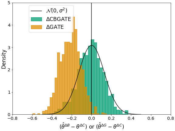
Figure C.1: N $=2,500$, correlated $Z$ and $X$

Figure C.2: N = 2500, uncorrelated $Z$ and $X$

Figure C.3: N = 10,000, correlated $Z$ and $X$

Figure C.4: N = 10,000, uncorrelated $Z$ and $X$

Note: These figures show the distribution of the bias of $\hat{\theta}^{\Delta C}$ and $\hat{\theta}^{\Delta G}$ compared to the true $\theta^{\Delta C}$. We plot a normal distribution to indicate convergence to an appropriately normal distribution. The figures are created using the results of the unconfoundedness setting and the DML estimator with the joint propensity score estimator.

Table C.3.4 shows the results for $N=2,500$ and $R=1,000$. The first block presents the results for the setting where there is selection into treatment and correlation between $Z$ and $X$. The second block depicts the results without correlating $Z$ and $X$. Estimating the effect ($\hat{\theta}^{\Delta C}$) with a joint propensity score (Specification 1) or with the product of two marginal propensity scores (Specification 2) leads to qualitatively similar results.

Table C.10: Simulation results: N = 2,500

max width=

No correlation between $Z$ and $X$    $\theta^{\Delta G}$ 1 0.278 -0.014 0.086 0.109 0.110 0.049 0.324 -0.000 94.10 79.50 $\theta^{\Delta C}$ 1 0.277 -0.011 0.088 0.110 0.110 -0.048 0.087 -0.001 94.30 79.80 $\theta^{\Delta C}$ 2 0.277 -0.017 0.087 0.109 0.110 -0.028 0.111 -0.001 94.50 79.20

• Note: This table shows results for $N=2,500$ and $R=1,000$ in two blocks: (1) correlation between $Z$ and $X$, and (2) no correlation between $Z$ and $X$. Column (1) shows the effect estimated, column (2) the respective version of the DML estimator used as explained in Table C.8 (3) the true effect. The remaining ten columns depict performance measures explained in C.1.

Table C.3.4 shows results for $N=10,000$ and $R=250$. Compared to the results with the smaller sample presented in Table C.3.4, the standard errors and the RMSE halve. This aligns with the convergence rate of a $\sqrt{N}$-consistent estimator.

Table C.11: Simulation results: N = 10,000

max width=

No correlation between $Z$ and $X$    $\theta^{\Delta G}$ 1 0.278 -0.008 0.045 0.055 0.055 0.199 0.064 -0.002 93.60 77.60 $\theta^{\Delta C}$ 1 0.277 -0.009 0.042 0.053 0.053 0.093 0.170 -0.001 94.00 78.00 $\theta^{\Delta C}$ 2 0.277 -0.010 0.043 0.053 0.054 0.114 0.217 -0.002 93.60 78.00

• Note: This table shows results for $N=10,500$ and $R=250$ in two blocks: (1) correlation between $Z$ and $X$, and (2) no correlation between $Z$ and $X$. Column (1) shows the effect estimated, column (2) the respective version of the DML estimator used as explained in Table C.8 (3) the true effect. The remaining ten columns depict performance measures explained in C.1.

Appendix D Appendix: Empirical example

D.1 Data descriptives

Table D.1 shows the mean and standard deviation of the covariates included in the analyses by treatment status. In addition to the covariates in this table, we add caseworkers’ fixed effects. For a more detailed description of the data and how the dataset was constructed, please see Knaus . (2022). The data can be accessed on swissubase.ch for research purposes.

Table D.1: Empirical analysis: Balance table for treatment and moderator variable

max width=0.95

4438 8607 30417 47877

• Note: This table shows the mean of some covariates included in the analysis. Column (1) and (2) show it for treated individuals, column (3) and (4) for non-treated individuals. Column (1) and (3) show it for non-Swiss individuals, column (2) and (4) for Swiss individuals.

Table D.1 shows the mean and standard deviation of the covariates included in the analyses by treatment status. In addition to the covariates in this table, we add caseworkers’ fixed effects. For a more detailed description of the data and how the dataset was constructed, please see Knaus . (2022). The data can be accessed on swissubase.ch for research purposes.

Table D.2: Empirical analysis: Balance table for treatment variable (participation in the programme)

max width=0.95

13,045       78,294

• Note: This table shows the mean and standard deviation of the covariates included in the analyses. Columns (1) and (2) show it for the treated group, columns (3) and (4) for the control group. The last column shows the standardised difference between the two groups. The standardized difference is calculated as $SD=\frac{\left|\bar{X}_{\text{treated}}-\bar{X}_{\text{control}}\right|}{\sqrt{1/2\left(\operatorname{Var}\left(\bar{X}_{\text{treated}}\right)+\operatorname{Var}\left(\bar{X}_{\text{control}}\right)\right)}}\cdot 100$ where $\bar{X}_{\text{treated}}$ and $\bar{X}_{\text{control}}$ indicate the sample mean of the treatment and control group, respectively.

Table D.1 shows descriptive statistics for Swiss and non-Swiss individuals for the other covariates. It can be seen that there are some differences in the covariates, namely in the mother tongue, past income, the previous job and the qualifications. Other variables such as age, place of residence or caseworker characteristics are well balanced.

Table D.3: Empirical analysis: Balance table for moderator variable (nationality)

max width=

34,855       56,484

• Note: This table shows the mean and standard deviation of some covariates included in the analysis. Column (1) and (2) show it for Swiss individuals, column (3) and (4) for non-Swiss individuals. The last column shows the standardised difference between the two groups. The standardized difference is calculated as $SD=\frac{\left|\bar{X}_{\text{Swiss}}-\bar{X}_{\text{non-Swiss}}\right|}{\sqrt{1/2\left(\operatorname{Var}\left(\bar{X}_{\text{Swiss}}\right)+\operatorname{Var}\left(\bar{X}_{\text{non-Swiss}}\right)\right)}}\cdot 100$ where $\bar{X}_{\text{Swiss}}$ and $\bar{X}_{\text{non-Swiss}}$ indicate the sample mean of the Non-Swiss and the Swiss individuals, respectively.

References

- Abrevaya \BOthers. (\APACyear2015) \APACinsertmetastarAbrevaya:2015{APACrefauthors}Abrevaya, J., Hsu, Y\BHBIC.\BCBL \BBA Lieli, R\BPBIP. \APACrefYearMonthDay2015. \BBOQ\APACrefatitleEstimating conditional average treatment effects Estimating conditional average treatment effects.\BBCQ \APACjournalVolNumPagesJournal of Business & Economic Statistics334485–505. \PrintBackRefs\CurrentBib
- Athey \BOthers. (\APACyear2019) \APACinsertmetastarAthey:2019{APACrefauthors}Athey, S., Tibshirani, J.\BCBL \BBA Wager, S. \APACrefYearMonthDay2019. \BBOQ\APACrefatitleGeneralized random forests Generalized random forests.\BBCQ \APACjournalVolNumPagesThe Annals of Statistics4721148–1178. \PrintBackRefs\CurrentBib
- Bansak (\APACyear2021) \APACinsertmetastarBansak:2021{APACrefauthors}Bansak, K. \APACrefYearMonthDay2021. \BBOQ\APACrefatitleEstimating causal moderation effects with randomized treatments and non-randomized moderators Estimating causal moderation effects with randomized treatments and non-randomized moderators.\BBCQ \APACjournalVolNumPagesJournal of the Royal Statistical Society: Series A (Statistics in Society)184165–86. \PrintBackRefs\CurrentBib
- Bansak \BOthers. (\APACyear2021) \APACinsertmetastarBansak:2021a{APACrefauthors}Bansak, K., Bechtel, M\BPBIM.\BCBL \BBA Margalit, Y. \APACrefYearMonthDay2021. \BBOQ\APACrefatitleWhy austerity? The mass politics of a contested policy Why austerity? The mass politics of a contested policy.\BBCQ \APACjournalVolNumPagesAmerican Political Science Review1152486–505. \PrintBackRefs\CurrentBib
- Bansak \BBA Nowacki (\APACyear2022) \APACinsertmetastarBansak:2022{APACrefauthors}Bansak, K.\BCBT \BBA Nowacki, T. \APACrefYearMonthDay2022. \BBOQ\APACrefatitleEffect Heterogeneity and Causal Attribution in Regression Discontinuity Designs Effect heterogeneity and causal attribution in regression discontinuity designs.\BBCQ \APACjournalVolNumPagesSocArXiv Papers. {APACrefURL} https://doi.org/10.31235/osf.io/vj34m \PrintBackRefs\CurrentBib
- Belloni \BBA Chernozhukov (\APACyear2013) \APACinsertmetastarBelloni:2013{APACrefauthors}Belloni, A.\BCBT \BBA Chernozhukov, V. \APACrefYearMonthDay2013. \BBOQ\APACrefatitleLeast squares after model selection in high-dimensional sparse models Least squares after model selection in high-dimensional sparse models.\BBCQ \APACjournalVolNumPagesBernoulli Society for Mathematical Statistics and Probability192521–547. \PrintBackRefs\CurrentBib
- Blackwell \BBA Olson (\APACyear2022) \APACinsertmetastarBlackwell:2021{APACrefauthors}Blackwell, M.\BCBT \BBA Olson, M\BPBIP. \APACrefYearMonthDay2022. \BBOQ\APACrefatitleReducing model misspecification and bias in the estimation of interactions Reducing model misspecification and bias in the estimation of interactions.\BBCQ \APACjournalVolNumPagesPolitical Analysis304495–514. \PrintBackRefs\CurrentBib
- Busso \BOthers. (\APACyear2014) \APACinsertmetastarBusso:2014{APACrefauthors}Busso, M., DiNardo, J.\BCBL \BBA McCrary, J. \APACrefYearMonthDay2014. \BBOQ\APACrefatitleNew evidence on the finite sample properties of propensity score reweighting and matching estimators New evidence on the finite sample properties of propensity score reweighting and matching estimators.\BBCQ \APACjournalVolNumPagesReview of Economics and Statistics965885–897. \PrintBackRefs\CurrentBib
- Chernozhukov, Chetverikov\BCBL \BOthers. (\APACyear2018) \APACinsertmetastarChernozhukov:2018{APACrefauthors}Chernozhukov, V., Chetverikov, D., Demirer, M., Duflo, E., Hansen, C., Newey, W.\BCBL \BBA Robins, J. \APACrefYearMonthDay2018. \BBOQ\APACrefatitleDouble/debiased machine learning for treatment and structural parameters Double/debiased machine learning for treatment and structural parameters.\BBCQ \APACjournalVolNumPagesThe Econometrics Journal211C1-C68. \PrintBackRefs\CurrentBib
- Chernozhukov, Fernández-Val\BCBL \BBA Luo (\APACyear2018) \APACinsertmetastarChernozhukov:2018b{APACrefauthors}Chernozhukov, V., Fernández-Val, I.\BCBL \BBA Luo, Y. \APACrefYearMonthDay2018. \BBOQ\APACrefatitleThe sorted effects method: Discovering heterogeneous effects beyond their averages The sorted effects method: Discovering heterogeneous effects beyond their averages.\BBCQ \APACjournalVolNumPagesEconometrica8661911–1938. \PrintBackRefs\CurrentBib
- Cockx \BOthers. (\APACyear2023) \APACinsertmetastarCockx:2023{APACrefauthors}Cockx, B., Lechner, M.\BCBL \BBA Bollens, J. \APACrefYearMonthDay2023. \BBOQ\APACrefatitlePriority to unemployed immigrants? A causal machine learning evaluation of training in Belgium Priority to unemployed immigrants? A causal machine learning evaluation of training in Belgium.\BBCQ \APACjournalVolNumPagesLabour Economics80102306. \PrintBackRefs\CurrentBib
- Davis \BBA Heller (\APACyear2017) \APACinsertmetastarDavis:2017{APACrefauthors}Davis, J\BPBIM.\BCBT \BBA Heller, S\BPBIB. \APACrefYearMonthDay2017. \BBOQ\APACrefatitleUsing causal forests to predict treatment heterogeneity: An application to summer jobs Using causal forests to predict treatment heterogeneity: An application to summer jobs.\BBCQ \APACjournalVolNumPagesAmerican Economic Review1075546–550. \PrintBackRefs\CurrentBib
- Dearing \BBA Hamilton (\APACyear2006) \APACinsertmetastarDearing:2006{APACrefauthors}Dearing, E.\BCBT \BBA Hamilton, L\BPBIC. \APACrefYearMonthDay2006. \BBOQ\APACrefatitleContemporary advances and classic advice for analyzing mediating and moderating variables Contemporary advances and classic advice for analyzing mediating and moderating variables.\BBCQ \APACjournalVolNumPagesMonographs of the Society for Research in Child Development71388–104. \PrintBackRefs\CurrentBib
- Fairchild \BBA McQuillin (\APACyear2010) \APACinsertmetastarFairchild:2010{APACrefauthors}Fairchild, A\BPBIJ.\BCBT \BBA McQuillin, S\BPBID. \APACrefYearMonthDay2010. \BBOQ\APACrefatitleEvaluating mediation and moderation effects in school psychology: A presentation of methods and review of current practice Evaluating mediation and moderation effects in school psychology: A presentation of methods and review of current practice.\BBCQ \APACjournalVolNumPagesJournal of School Psychology48153–84. \PrintBackRefs\CurrentBib
- Farbmacher \BOthers. (\APACyear2022) \APACinsertmetastarFarbmacher:2022{APACrefauthors}Farbmacher, H., Huber, M., Lafférs, L., Langen, H.\BCBL \BBA Spindler, M. \APACrefYearMonthDay2022. \BBOQ\APACrefatitleCausal mediation analysis with double machine learning Causal mediation analysis with double machine learning.\BBCQ \APACjournalVolNumPagesThe Econometrics Journal252277–300. \PrintBackRefs\CurrentBib
- Farrell \BOthers. (\APACyear2021) \APACinsertmetastarFarrell:2021{APACrefauthors}Farrell, M\BPBIH., Liang, T.\BCBL \BBA Misra, S. \APACrefYearMonthDay2021. \BBOQ\APACrefatitleDeep neural networks for estimation and inference Deep neural networks for estimation and inference.\BBCQ \APACjournalVolNumPagesEconometrica891181–213. \PrintBackRefs\CurrentBib
- Foster \BBA Syrgkanis (\APACyear2023) \APACinsertmetastarFoster:2023{APACrefauthors}Foster, D\BPBIJ.\BCBT \BBA Syrgkanis, V. \APACrefYearMonthDay2023. \BBOQ\APACrefatitleOrthogonal statistical learning Orthogonal statistical learning.\BBCQ \APACjournalVolNumPagesThe Annals of Statistics513879–908. \PrintBackRefs\CurrentBib
- Frazier \BOthers. (\APACyear2004) \APACinsertmetastarFrazier:2004{APACrefauthors}Frazier, P\BPBIA., Tix, A\BPBIP.\BCBL \BBA Barron, K\BPBIE. \APACrefYearMonthDay2004. \BBOQ\APACrefatitleTesting moderator and mediator effects in counseling psychology research. Testing moderator and mediator effects in counseling psychology research.\BBCQ \APACjournalVolNumPagesJournal of Counseling Psychology511115. \PrintBackRefs\CurrentBib
- Gogineni \BOthers. (\APACyear1995) \APACinsertmetastarGogineni:1995{APACrefauthors}Gogineni, A., Alsup, R.\BCBL \BBA Gillespie, D\BPBIF. \APACrefYearMonthDay1995. \BBOQ\APACrefatitleMediation and moderation in social work research Mediation and moderation in social work research.\BBCQ \APACjournalVolNumPagesSocial Work Research19157–63. \PrintBackRefs\CurrentBib
- Hines \BOthers. (\APACyear2022) \APACinsertmetastarHines:2022{APACrefauthors}Hines, O., Dukes, O., Diaz-Ordaz, K.\BCBL \BBA Vansteelandt, S. \APACrefYearMonthDay2022. \BBOQ\APACrefatitleDemystifying statistical learning based on efficient influence functions Demystifying statistical learning based on efficient influence functions.\BBCQ \APACjournalVolNumPagesThe American Statistician763292–304. \PrintBackRefs\CurrentBib
- Huber \BOthers. (\APACyear2013) \APACinsertmetastarHuber:2013{APACrefauthors}Huber, M., Lechner, M.\BCBL \BBA Wunsch, C. \APACrefYearMonthDay2013. \BBOQ\APACrefatitleThe performance of estimators based on the propensity score The performance of estimators based on the propensity score.\BBCQ \APACjournalVolNumPagesJournal of Econometrics17511–21. \PrintBackRefs\CurrentBib
- Imbens (\APACyear2004) \APACinsertmetastarImbens:2004{APACrefauthors}Imbens, G\BPBIW. \APACrefYearMonthDay2004. \BBOQ\APACrefatitleNonparametric estimation of average treatment effects under exogeneity: A review Nonparametric estimation of average treatment effects under exogeneity: A review.\BBCQ \APACjournalVolNumPagesReview of Economics and statistics8614–29. \PrintBackRefs\CurrentBib
- Imbens \BBA Wooldridge (\APACyear2009) \APACinsertmetastarImbens:2009{APACrefauthors}Imbens, G\BPBIW.\BCBT \BBA Wooldridge, J\BPBIM. \APACrefYearMonthDay2009. \BBOQ\APACrefatitleRecent developments in the econometrics of program evaluation Recent developments in the econometrics of program evaluation.\BBCQ \APACjournalVolNumPagesJournal of Economic Literature4715–86. \PrintBackRefs\CurrentBib
- Kennedy (\APACyear2022) \APACinsertmetastarKennedy:2022{APACrefauthors}Kennedy, E\BPBIH. \APACrefYearMonthDay2022. \BBOQ\APACrefatitleSemiparametric doubly robust targeted double machine learning: A review Semiparametric doubly robust targeted double machine learning: A review.\BBCQ \APACjournalVolNumPagesarXiv preprint arXiv:2203.06469. \PrintBackRefs\CurrentBib
- Kennedy (\APACyear2023) \APACinsertmetastarKennedy:2023{APACrefauthors}Kennedy, E\BPBIH. \APACrefYearMonthDay2023. \BBOQ\APACrefatitleTowards optimal doubly robust estimation of heterogeneous causal effects Towards optimal doubly robust estimation of heterogeneous causal effects.\BBCQ \APACjournalVolNumPagesarXiv preprint arXiv:2004.14497. \PrintBackRefs\CurrentBib
- Kennedy \BOthers. (\APACyear2017) \APACinsertmetastarKennedy:2017{APACrefauthors}Kennedy, E\BPBIH., Ma, Z., McHugh, M\BPBID.\BCBL \BBA Small, D\BPBIS. \APACrefYearMonthDay2017. \BBOQ\APACrefatitleNon-parametric methods for doubly robust estimation of continuous treatment effects Non-parametric methods for doubly robust estimation of continuous treatment effects.\BBCQ \APACjournalVolNumPagesJournal of the Royal Statistical Society. Series B (Statistical Methodology)7941229–1245. \PrintBackRefs\CurrentBib
- Knaus (\APACyear2022) \APACinsertmetastarKnaus:2022b{APACrefauthors}Knaus, M\BPBIC. \APACrefYearMonthDay2022. \BBOQ\APACrefatitleDouble machine learning-based programme evaluation under unconfoundedness Double machine learning-based programme evaluation under unconfoundedness.\BBCQ \APACjournalVolNumPagesThe Econometrics Journal253602–627. \PrintBackRefs\CurrentBib
- Knaus \BOthers. (\APACyear2021) \APACinsertmetastarKnaus:2021{APACrefauthors}Knaus, M\BPBIC., Lechner, M.\BCBL \BBA Strittmatter, A. \APACrefYearMonthDay2021. \BBOQ\APACrefatitleMachine learning estimation of heterogeneous causal effects: Empirical Monte Carlo evidence Machine learning estimation of heterogeneous causal effects: Empirical Monte Carlo evidence.\BBCQ \APACjournalVolNumPagesThe Econometrics Journal241134–161. \PrintBackRefs\CurrentBib
- Knaus \BOthers. (\APACyear2022) \APACinsertmetastarKnaus:2022{APACrefauthors}Knaus, M\BPBIC., Lechner, M.\BCBL \BBA Strittmatter, A. \APACrefYearMonthDay2022. \BBOQ\APACrefatitleHeterogeneous employment effects of job search programmes: A machine learning approach Heterogeneous employment effects of job search programmes: A machine learning approach.\BBCQ \APACjournalVolNumPagesJournal of Human Resources572597–636. \PrintBackRefs\CurrentBib
- Künzel \BOthers. (\APACyear2019) \APACinsertmetastarKuenzel:2019{APACrefauthors}Künzel, S\BPBIR., Sekhon, J\BPBIS., Bickel, P\BPBIJ.\BCBL \BBA Yu, B. \APACrefYearMonthDay2019. \BBOQ\APACrefatitleMetalearners for estimating heterogeneous treatment effects using machine learning Metalearners for estimating heterogeneous treatment effects using machine learning.\BBCQ \APACjournalVolNumPagesProceedings of the national academy of sciences116104156–4165. \PrintBackRefs\CurrentBib
- Lechner \BOthers. (\APACyear2020) \APACinsertmetastarKnaus:2020{APACrefauthors}Lechner, M., Knaus, M\BPBIC., Huber, M., Frölich, M., Behncke, S., Mellace, G.\BCBL \BBA Strittmatter, A. \APACrefYearMonthDay2020. \BBOQ\APACrefatitleSwiss Active Labor Market Policy Evaluation [Dataset] Swiss Active Labor Market Policy Evaluation [Dataset].\BBCQ \APACjournalVolNumPagesDistributed by FORS, Lausanne. {APACrefURL} https://doi.org/10.23662/FORS-DS-1203-1 \PrintBackRefs\CurrentBib
- Lechner \BBA Mareckova (\APACyear2022) \APACinsertmetastarLechner:2022{APACrefauthors}Lechner, M.\BCBT \BBA Mareckova, J. \APACrefYearMonthDay2022. \BBOQ\APACrefatitleModified Causal Forest Modified causal forest.\BBCQ \APACjournalVolNumPagesarXiv preprint arXiv:2209.03744. \PrintBackRefs\CurrentBib
- Luo \BOthers. (\APACyear2016) \APACinsertmetastarLuo:2016{APACrefauthors}Luo, Y., Spindler, M.\BCBL \BBA Kück, J. \APACrefYearMonthDay2016. \BBOQ\APACrefatitleHigh-Dimensional Boosting: Rate of Convergence High-dimensional boosting: Rate of convergence.\BBCQ \APACjournalVolNumPagesarXiv preprint arXiv:1602.08927. \PrintBackRefs\CurrentBib
- Marsh \BOthers. (\APACyear2013) \APACinsertmetastarMarsh:2013{APACrefauthors}Marsh, H\BPBIW., Hau, K\BHBIT., Wen, Z., Nagengast, B.\BCBL \BBA Morin, A\BPBIJ. \APACrefYearMonthDay2013. \BBOQ\APACrefatitleModeration. Moderation.\BBCQ \BIn \APACrefbtitleThe Oxford handbook of quantitative methods: Statistical analysis The Oxford handbook of quantitative methods: Statistical analysis (\BPGS 361–386). \APACaddressPublisherOxford University Press. \PrintBackRefs\CurrentBib
- Nie \BBA Wager (\APACyear2021) \APACinsertmetastarNie:2021{APACrefauthors}Nie, X.\BCBT \BBA Wager, S. \APACrefYearMonthDay2021. \BBOQ\APACrefatitleQuasi-oracle estimation of heterogeneous treatment effects Quasi-oracle estimation of heterogeneous treatment effects.\BBCQ \APACjournalVolNumPagesBiometrika1082299–319. \PrintBackRefs\CurrentBib
- Rambachan \BOthers. (\APACyear2022) \APACinsertmetastarRambachan:2022{APACrefauthors}Rambachan, A., Coston, A.\BCBL \BBA Kennedy, E. \APACrefYearMonthDay2022. \BBOQ\APACrefatitleCounterfactual risk assessments under unmeasured confounding Counterfactual risk assessments under unmeasured confounding.\BBCQ \APACjournalVolNumPagesarXiv preprint arXiv:2212.09844. \PrintBackRefs\CurrentBib
- Rose \BOthers. (\APACyear2004) \APACinsertmetastarRose:2004{APACrefauthors}Rose, B\BPBIM., Holmbeck, G\BPBIN., Coakley, R\BPBIM.\BCBL \BBA Franks, E\BPBIA. \APACrefYearMonthDay2004. \BBOQ\APACrefatitleMediator and moderator effects in developmental and behavioral pediatric research Mediator and moderator effects in developmental and behavioral pediatric research.\BBCQ \APACjournalVolNumPagesJournal of Developmental & Behavioral Pediatrics25158–67. \PrintBackRefs\CurrentBib
- Rubin (\APACyear1974) \APACinsertmetastarRubin:1974{APACrefauthors}Rubin, D\BPBIB. \APACrefYearMonthDay1974. \BBOQ\APACrefatitleEstimating causal effects of treatments in randomized and nonrandomized studies. Estimating causal effects of treatments in randomized and nonrandomized studies.\BBCQ \APACjournalVolNumPagesJournal of Educational Psychology665688. \PrintBackRefs\CurrentBib
- Sant’Anna \BBA Zhao (\APACyear2020) \APACinsertmetastarSantAnna:2020{APACrefauthors}Sant’Anna, P\BPBIH.\BCBT \BBA Zhao, J. \APACrefYearMonthDay2020. \BBOQ\APACrefatitleDoubly robust difference-in-differences estimators Doubly robust difference-in-differences estimators.\BBCQ \APACjournalVolNumPagesJournal of Econometrics2191101–122. \PrintBackRefs\CurrentBib
- Semenova \BBA Chernozhukov (\APACyear2021) \APACinsertmetastarSemenova:2021{APACrefauthors}Semenova, V.\BCBT \BBA Chernozhukov, V. \APACrefYearMonthDay2021. \BBOQ\APACrefatitleDebiased machine learning of conditional average treatment effects and other causal functions Debiased machine learning of conditional average treatment effects and other causal functions.\BBCQ \APACjournalVolNumPagesThe Econometrics Journal242264–289. \PrintBackRefs\CurrentBib
- Smucler \BOthers. (\APACyear2019) \APACinsertmetastarSmucler:2019{APACrefauthors}Smucler, E., Rotnitzky, A.\BCBL \BBA Robins, J\BPBIM. \APACrefYearMonthDay2019. \BBOQ\APACrefatitleA unifying approach for doubly-robust regularized estimation of causal contrasts A unifying approach for doubly-robust regularized estimation of causal contrasts.\BBCQ \APACjournalVolNumPagesarXiv preprint arXiv:1904.03737. \PrintBackRefs\CurrentBib
- Syrgkanis \BBA Zampetakis (\APACyear2020) \APACinsertmetastarSyrgkanis:2020{APACrefauthors}Syrgkanis, V.\BCBT \BBA Zampetakis, M. \APACrefYearMonthDay2020. \BBOQ\APACrefatitleEstimation and inference with trees and forests in high dimensions Estimation and inference with trees and forests in high dimensions.\BBCQ \BIn \APACrefbtitleConference on learning theory Conference on learning theory (\BPGS 3453–3454). \PrintBackRefs\CurrentBib
- Tian \BOthers. (\APACyear2014) \APACinsertmetastarTian:2014{APACrefauthors}Tian, L., Alizadeh, A\BPBIA., Gentles, A\BPBIJ.\BCBL \BBA Tibshirani, R. \APACrefYearMonthDay2014. \BBOQ\APACrefatitleA simple method for estimating interactions between a treatment and a large number of covariates A simple method for estimating interactions between a treatment and a large number of covariates.\BBCQ \APACjournalVolNumPagesJournal of the American Statistical Association1095081517–1532. \PrintBackRefs\CurrentBib
- Wager (\APACyear2020) \APACinsertmetastarWager:2020{APACrefauthors}Wager, S. \APACrefYearMonthDay2020. \APACrefbtitleSTATS 361: Causal Inference. STATS 361: Causal Inference. {APACrefURL} https://web.stanford.edu/~swager/stats361.pdf \PrintBackRefs\CurrentBib
- Wager \BBA Athey (\APACyear2018) \APACinsertmetastarWager:2018{APACrefauthors}Wager, S.\BCBT \BBA Athey, S. \APACrefYearMonthDay2018. \BBOQ\APACrefatitleEstimation and inference of heterogeneous treatment effects using random forests Estimation and inference of heterogeneous treatment effects using random forests.\BBCQ \APACjournalVolNumPagesJournal of the American Statistical Association1135231228–1242. \PrintBackRefs\CurrentBib
- Wager \BBA Walther (\APACyear2015) \APACinsertmetastarWager:2015{APACrefauthors}Wager, S.\BCBT \BBA Walther, G. \APACrefYearMonthDay2015. \BBOQ\APACrefatitleAdaptive concentration of regression trees, with application to random forests Adaptive concentration of regression trees, with application to random forests.\BBCQ \APACjournalVolNumPagesarXiv preprint arXiv:1503.06388. \PrintBackRefs\CurrentBib
- Zimmert (\APACyear2018) \APACinsertmetastarZimmert:2018{APACrefauthors}Zimmert, M. \APACrefYearMonthDay2018. \BBOQ\APACrefatitleEfficient difference-in-differences estimation with high-dimensional common trend confounding Efficient difference-in-differences estimation with high-dimensional common trend confounding.\BBCQ \APACjournalVolNumPagesarXiv preprint arXiv:1809.01643. \PrintBackRefs\CurrentBib
- Zimmert \BBA Lechner (\APACyear2019) \APACinsertmetastarZimmert:2019{APACrefauthors}Zimmert, M.\BCBT \BBA Lechner, M. \APACrefYearMonthDay2019. \BBOQ\APACrefatitleNonparametric estimation of causal heterogeneity under high-dimensional confounding Nonparametric estimation of causal heterogeneity under high-dimensional confounding.\BBCQ \APACjournalVolNumPagesForthcoming in the Econometrics Journal. \PrintBackRefs\CurrentBib