On the origins of CMB anomalies and testing a new theory of inflationary quantum fluctuations

Abstract

In this paper, we present compelling evidence suggesting a statistical violation of parity symmetry (a discrete symmetry that is separate from isotropy) in the Cosmic Microwave Background (CMB) map, measured through two-point temperature correlations. Any asymmetry associated with discrete symmetries, such as parity, challenges our understanding of quantum physics associated with primordial physics rather than LCDM ($\Lambda$ Cold-Dark-Matter) itself. We commence by conducting a comprehensive analysis of the Planck CMB, focusing on the distribution of power in low-multipoles and temperature anticorrelations at parity conjugate points in position space. We find tension with the near scale-invariant power-law power spectrum of Standard Inflation (SI), with p-values of the order ${\mathcal{O}}\left(10^{-4}-10^{-3}\right)$. Subsequently, we explore the recently proposed direct-sum inflation (DSI), where a quantum fluctuation arises as a direct sum of two components evolving forward and backward in time at parity conjugate points in physical space. This mechanism results in a parity-asymmetric scale-dependent power spectrum, particularly prominent at low-multipoles, without any additional free model parameters. Our findings indicate that DSI is consistent with data on parity asymmetry, the absence of power at $\theta>60^{\circ}$, and power suppression at low-even-multipoles which are major data anomalies in the SI model. Furthermore, we discover that the parameters characterizing the hemispherical power asymmetry anomaly become statistically insignificant when the large SI quadrupole amplitude is reduced to align with the data. DSI explains this low quadrupole with a p-value of 3.5%, 39 times higher than SI. Combining statistics from parameters measuring parity and low-$\ell$ angular power spectrum, we find that DSI is 50-650 times more probable than SI. In summary, our investigation suggests that while CMB temperature fluctuations exhibit homogeneity and isotropy, they also display parity-violating behavior consistent with predictions of DSI. This observation provides a tantalizing evidence for the quantum mechanical nature of gravity.

1 Introduction

The 20th century witnessed the emergence of two profoundly successful theories, General Relativity (GR) and Quantum Mechanics (QM), each excelling in explaining the macroscopic and microscopic realms, respectively. Additionally, the Standard Model (SM) of particle physics stands as a significant achievement, resulting from the successful integration of Quantum Mechanics with special relativity in the form of Quantum Field Theory (QFT). The discrete symmetries such as charge conjugation (${\mathcal{C}}$), Parity (${\mathcal{P}}$), and time-reversal (${\mathcal{T}}$) played a vital role in understanding and testing SM of particle physics. For example, the Parity violation observed as asymmetric angular distribution of electron emission ($\beta-$ decay) in Cobalt-60 Lee:1956qn ; Wu:1957my ; Christenson:1964fg , the ${\mathcal{C}}{\mathcal{P}}$-violation in the weak interactions and the ${\mathcal{C}}{\mathcal{P}}{\mathcal{T}}$ invariance of scattering amplitudes Coleman:2018mew . Moreover, ${\mathcal{C}}{\mathcal{P}}$-violation has been identified as a potential explanation for the observed particle-antiparticle asymmetry in the Universe. This observation strongly suggests the necessity of extending beyond the SM of particle physics Sakharov:1967dj ; Canetti:2012zc ; Kaufman:2014rpa . It’s important to note that discrete operations like ${\mathcal{C}},{\mathcal{P}},{\mathcal{T}}$ are intricately linked to quantum rather than classical physics. Gravity stands out as the weakest among all fundamental forces in nature. The exploration of the status of discrete symmetries in quantum gravity or for quantum fields in curved spacetime naturally arises as a fundamental question. A definitive answer to this inquiry is pivotal for constructing a comprehensive theory of quantum gravity that remains valid up to Planck scales and beyond.

Parity is an inherent characteristic of elementary particles and antiparticles. The Parity transformation ${\mathcal{P}}$, combined with charge conjugation ${\mathcal{C}}$—both being unitary operations Coleman:2018mew —transforms a particle into its corresponding antiparticle while flipping the sign of the momenta. In contrast, the time reversal operation is anti-unitary, counteracting the effects of ${\mathcal{P}}$ by reversing the sign of physical momenta. In the realm of quantum gravity, particularly when addressing the early Universe’s cosmology, such as the cosmic microwave background (CMB), the evolution of spacetime geometry transitions from quantum to classical. In this context, the concept of Parity asymmetry suggests differences in physics at Parity conjugate points. Classical GR portrays spacetime as dynamical entity, and understanding time reversal for quantum fields propagating in classical spacetime poses a non-trivial challenge.

This paper delves into the foundational understanding of parity and time reversal in quantum gravity, revealing compelling observational evidence in the latest CMB data. Additionally, the paper rigorously reevaluates the status of CMB anomalies, specifically the so-called Hemispherical Power Asymmetry (HPA), often considered as a violation of the cosmological principle Land:2005ad ; Hoftuft:2009rq ; Mukherjee:2015mma ; Akrami:2014eta ; Jones:2023ncn . The findings indicate no significant statistical evidence supporting the existence of HPA, thus challenging previous claims associated with cosmological principle violations.

The paper is organized as follows. In Sec. 2 we present a visual picture of CMB’s parity asymmetry which has been consistently observed over the last 3 decades. We also show that a better way to characterize the parity asymmetry is through temperature anticorrelation maps of the CMB data. In Sec. 3 we discuss what could be the primordial (quantum) physics in the scope of inflationary cosmology that can lead to the parity asymmetric feature of CMB. We present an intuitive discussion on the idea of direct-sum inflation (DSI) where quantum fluctuations during inflation contain a parity asymmetric time evolution which leaves it in the LSS once they become classical. In Sec. 4 we study the probabilities of SI and DSI given the CMB data and vice versa using the observables that characterize only parity and not isotropy both in configuration space and also in the harmonic space. We record our results in terms of the p-values which give the best description for the SI and DSI models in terms of fitting the data. In Sec. 5 we establish a connection between lower power in the quadrupole and the observed lack of correlations at angular scales $\theta>60^{\circ}$. Then we analyze the probability of DSI explaining the lack of power on large scales compared to SI. In Sec. 6 we examine the HPA and related observables with a new set of simulations that test further the statistical significance of HPA. Also, we assess if the lower quadrupole observed in the data can influence the significance of HPA. In Sec. 7 we present in detail the SI and fundamental questions that lead to the DSI framework. We also calculate the parity-asymmetric angular power spectrum in DSI which has been used in testing the model with the Planck CMB data. We discuss the implications of DSI to Stochastic inflation and vice versa. We also comment on how our observational tests of DSI can provide valuable input to the stochastic framework of inflationary quantum fluctuations and the issue of quantum-to-classical transition. We also elucidate how the DSI predictions for parity-asymmetric CMB remain stable concerning the tiny modifications in the coarse-graining scale of stochastic inflation. We end with Conclusions and outlook, followed by some Appendixes.

In Appendix A we present how we make the parity conjugate maps of CMB data with an illustration of the parity conjugate map of Earth. In Appendix B, we provide an explanation and quantification of the sampling variance related to the angular power spectra $C_{\ell}$ for both the data and the models. We explicitly demonstrate that the distribution of the sampling variance of $C_{\ell}$ is non-Gaussian, making the conversion of $\chi^{2}$ values to probabilities challenging. Additionally, we present the covariant matrix of $C_{\ell}$ for low $\ell$. Appendix C is dedicated to a discussion of our CMB simulations, noise considerations, and the impact of using masks on the data sets of the Planck satellite. In Appendix D, we delve into the observables associated with the absence of correlations at large angular scales. In Appendix E, we conduct a visual comparison of CMB maps with DSI and SI simulations. Furthermore, we present simulated maps for HPA to visually distinguish anisotropy and parity asymmetric CMB maps.

1.1 Conventions, Notations and Data analysis:

Throughout the paper, we follow the metric signature of mostly positive. We work in the units of $\hbar=c=1$ and $M_{p}^{2}=\frac{1}{\sqrt{8\pi G}}=1$. Often in observations ${\mathcal{T}}(\hat{n})$ is given in units of Kelvin (K) or micro-Kelvin $\mu$K instead of units of $T_{0}$. In all the paper, we will therefore normalize ${\mathcal{T}}(\hat{n})$ to $\sigma_{\mathcal{T}}\equiv\sqrt{<{\mathcal{T}}(\hat{n})^{2}>}$ (where the average $<\dots>$ is overall sky directions) so that ${\mathcal{T}}(\hat{n})$ becomes a dimensionless scalar field of unit variance. This is because our study is not about the overall amplitude of fluctuations, but only their symmetrical properties. In the whole paper, we only speak about point-parity which is a discrete transformation $\textbf{x}\to-\textbf{x}$ or $\left(\theta,\,\varphi\right)\to\left(\pi-\theta,\,\pi+\varphi\right)$ in spherical coordinates. Whenever we say CMB angular power spectrum, it only means in the context of two-point temperature correlations. In this paper, we will use the data maps, masks, and best-fit LCDM model provided by Planck 2018 data release. We focus on the component-separated Commander (COMM_m from now on), SMICA (SMIC_m), SEVEM (SEVE_m) and NILC (NILC_m). The subscript ’$m$’ in the name indicates that we use the mask corresponding to each component separation, which is the default. The fraction of unmasked sky is: $f_{sky}=88.8,84.2,83.8$ and $78.6\%$ respectively for $N_{side}=2048$. The subscript ’$c$’ indicates that we use the common mask which covers $77.9\%$ of the sky. We do not use the CMB measurement inside the mask as they are contaminated and have different noise properties. To study the parity asymmetry of the CMB map and visualizations of data and theoretical model realizations, we used HEALPix software with further details explained in Appendix. A.

2 The parity asymmetric cosmic microwave background (CMB)

The observation of CMB from Cosmic Microwave Background Explorer (COBE) satellite in 1992 has revealed for the first time the blueprint of large-scale structure (LSS) of the Universe with temperature fluctuations of the order $\frac{\Delta T}{\bar{T}}\sim 10^{-5}$ with Gaussian distribution of two-point correlations revealing the large scale homogeneous and isotropic nature of primordial Universe COBEw2 ; Julien . COBE Sattelite has particularly measured the CMB anisotropies at angular scales $\theta\gtrsim 6^{\circ}$ which corresponds to the low-multipoles $\ell\lesssim 30$. The successors of COBE measurements in the later decades are carried by the Wilkinson Microwave Anisotropy Probe (WMAP) and Planck Satellites. They have confirmed the near-scale invariant spectrum of primordial fluctuations at small angular scales $\theta<1^{\circ}$ leaving the large-scale anomalies at low-multipoles Schwarz:2015cma . First of all, CMB sky is on average homogeneous and isotropic and the CMB temperature fluctuations being one part in $10^{5}$ is the first hint to speculate their origin must be spacetime fluctuations around the Friedman-Lemaître-Robertson-Walker (FLRW) Universe. CMB temperature sky fluctuations $\Delta T$ within an isotropic background of mean temperature $T_{0}$ can be characterized by the local (configuration space) scalar field ${\mathcal{T}}(\hat{n})$ or its Fourier counterpart, which in spherical coordinates is the harmonic $a_{\ell m}$ decomposition: Durrer:2008eom

$${\mathcal{T}}\left(\hat{n}\right)\equiv\frac{\Delta T\left(\hat{n}\right)}{T_{0}}=\sum a_{\ell m}Y_{\ell m}\left(\hat{n}\right)\quad;\quad a_{\ell m}=\int d\Omega\,Y_{\ell m}^{\ast}\left(\hat{n}\right){\mathcal{T}}\left(\hat{n}\right)\,.$$ (1)

where the multipole $\ell=0,1,\dots,\ell_{max}$ corresponds to the inverse angular separation $\theta$ of each mode: $\ell\simeq\pi/\theta$ (e.g. $\ell_{max}\sim\pi/\theta_{min}$ corresponds to the map resolution $\theta_{min}$) and $m=-\ell\dots\ell$ is the direction $\hat{\theta}$ of each mode (see Fig. 1 for an illustration).

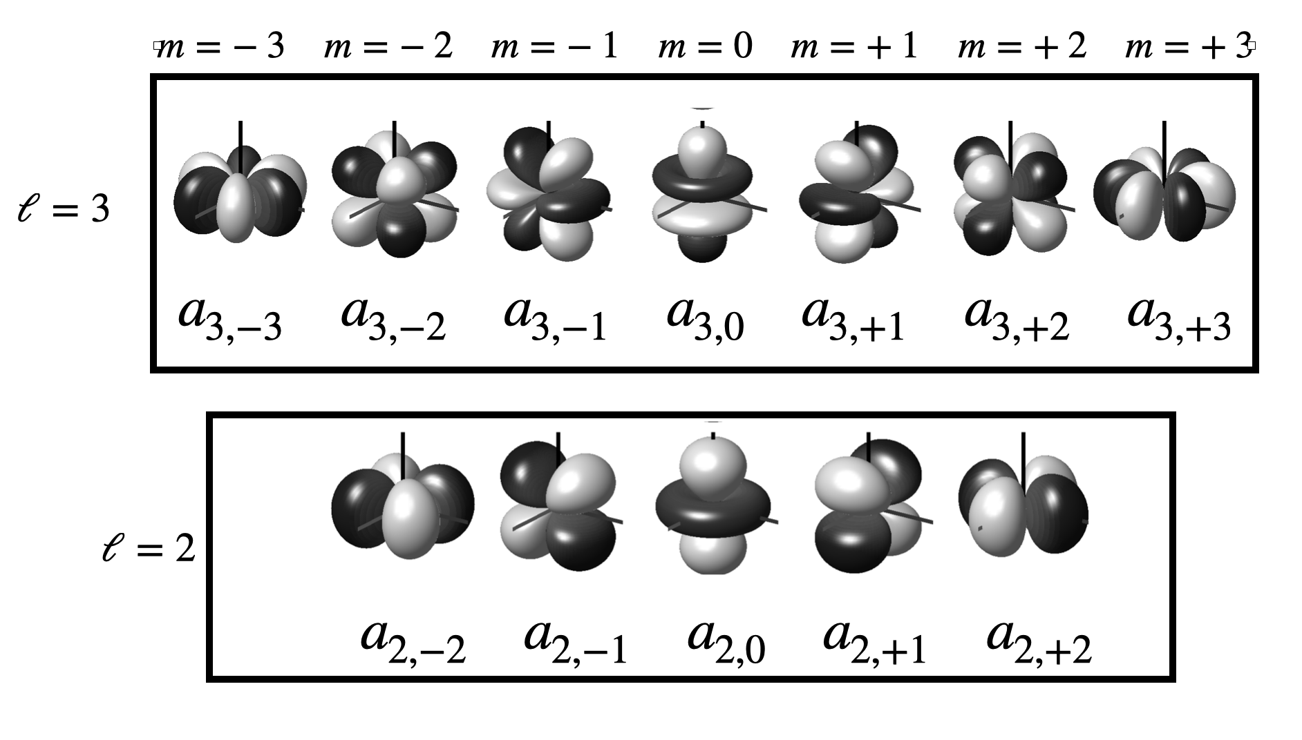
Figure 1: Representation of Spherical harmonic functions $Y_{\ell m}$ with the corresponding $a_{\ell m}$ coefficients for the quadrupole ($\ell=2$) and octopole ($\ell=3$). Note the even (odd) spherical ${\mathcal{P}}$ conjugate parity of $\ell=2$ ($\ell=3$).

In the flat sky limit (i.e. small angles) we have that the 2D Fourier modes are $\hat{k}=\ell e^{i\pi m/\ell}$. The CMB angular TT power spectrum is usually defined as:

$$C_{\ell}=\frac{1}{2\ell+1}\sum_{m}|a_{\ell m}|^{2}\,.$$ (2)

but often displayed as $D_{\ell}\equiv\ell(\ell+1)\,C_{\ell}/2\pi$, corresponding to the variance in each mode $\ell$.

We can decompose the CMB temperature fluctuation ${\mathcal{T}}(\hat{n})$ as the sum of its symmetric (even parity) ${\mathcal{T}}^{+}(\hat{n})$ and its antisymmetric (odd parity) ${\mathcal{T}}^{-}(\hat{n})$ components:

$${\mathcal{T}}(\hat{n})={\mathcal{T}}^{+}(\hat{n})+{\mathcal{T}}^{-}(\hat{n})$$ (3)

where

$${\mathcal{T}}^{+}(\hat{n})\equiv\frac{1}{2}\left[{\mathcal{T}}(\hat{n})+{\mathcal{T}}(-\hat{n})\right]$$ (4)

$${\mathcal{T}}^{-}(\hat{n})\equiv\frac{1}{2}\left[{\mathcal{T}}(\hat{n})-{\mathcal{T}}(-\hat{n})\right]$$

where $(-\hat{n})$ is the antipodal direction or parity ${\mathcal{P}}$ conjugate of $(\hat{n})$. From the SMICA map of Planck data Planck:2019evm we create the projections of Symmetric (S or ${\mathcal{T}}^{+}$) and antisymmetric (A or ${\mathcal{T}}^{-}$) parts in Fig. 2. Here, we can witness that the antisymmetric map (A) and the symmetric map (S) contain large-scale structures whose shapes are ${\mathcal{P}}$ conjugate images of each other. However, the remarkable revelation here is that the total map (A+S) appears very close to the antisymmetric map (A) meaning that the CMB is odd parity preferred than even. This is exactly what we call in the rest of the paper parity asymmetry that we show that can emerge from quantum fluctuations during early Universe inflationary expansion. The odd parity favored CMB map in Fig. 2 implies that the temperature fluctuation of the CMB contains an additional purely antisymmetric component

$${\mathcal{T}}\left(\hat{n}\right)=\tilde{{\mathcal{T}}}\left(\hat{n}\right)+\Delta{\mathcal{T}}\left(\hat{n}\right)$$ (5)

where $\bar{{\mathcal{T}}}(\hat{n})$ is neither symmetric nor antisymmetric. This component $\Delta{\mathcal{T}}\left(\hat{n}\right)$ satisfies the purely antisymmetric property

$$\Delta{\mathcal{T}}\left(\hat{n}\right)=-\Delta{\mathcal{T}}\left(-\hat{n}\right)\,.$$ (6)

It is this, additional component that makes the CMB map (A+S) look more like A than S as we see in Fig. 2. If $\Delta{\mathcal{T}}\left(\hat{n}\right)=0$ then there is no defined parity, we expect even and odd multipoles to be similar. But this is not what we see in the data, the CMB strongly aligned towards the odd parity. We carry out further analysis of this in the upcoming sections.

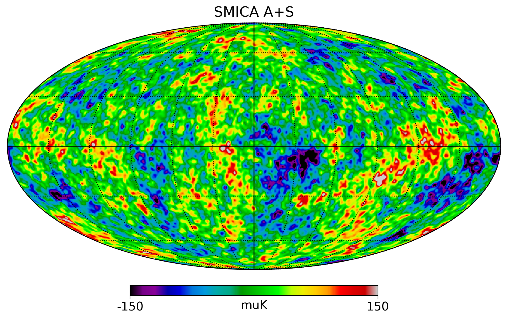
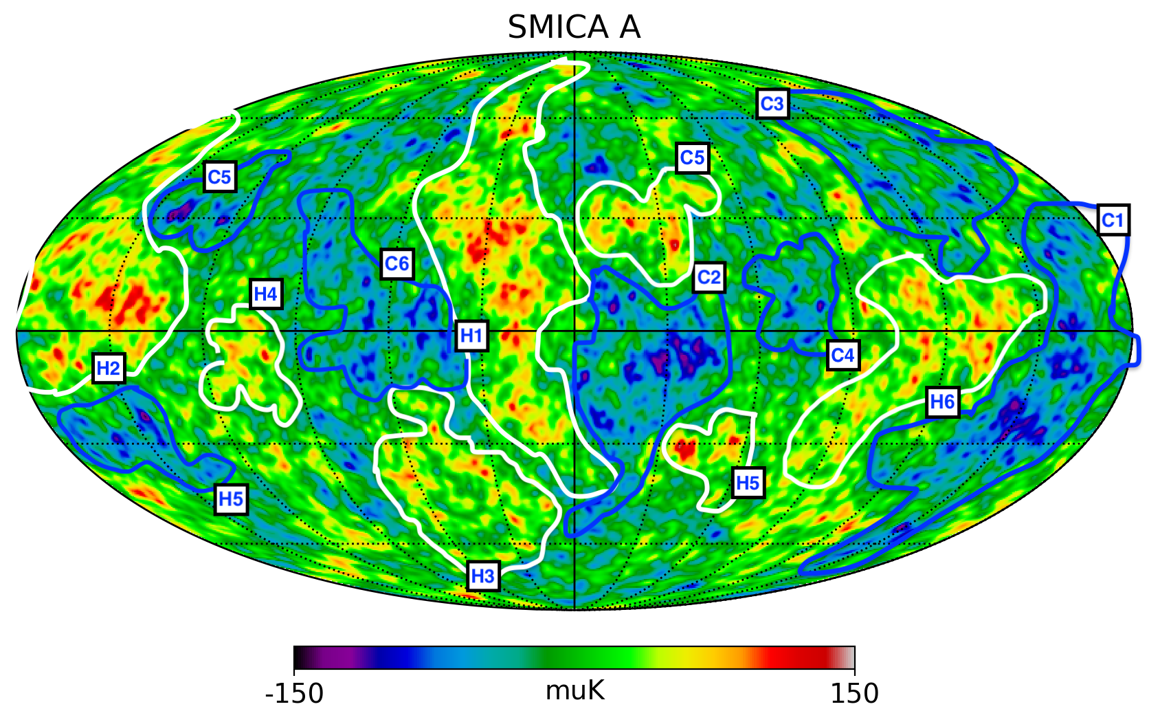
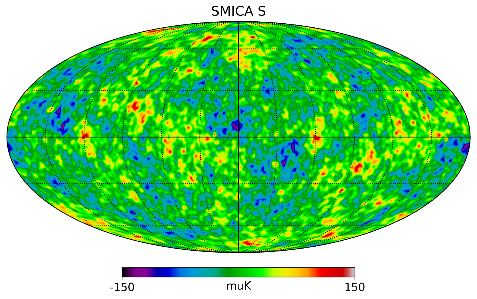
Figure 2: The Mollview projections above display the antisymmetric (A or ${\mathcal{T}}^{-}$, middle) and symmetric (S or ${\mathcal{T}}^{+}$, bottom) decomposition of the Planck 2018 map (SMICA, top). The mirror (odd/even parity) symmetry is readily apparent. Notably, large-scale cold structures crossing the galactic plane from the Southern Galactic Cap (SGC) to the North (labeled C1) have corresponding hot (antisymmetric) mirror structures (labeled H1) crossing the opposite side of the galactic plane from the Northern Galactic Cap (NGC) to the South. This symmetry holds for structures C2, C3, C4, and C5 as well. These structures align closely with the original SMICA map (A+S) and are either entirely or partially absent in the $T^{+}$ even parity map, indicating that they are genuine odd parity components. In contrast, the very hot superstructure around H6, just above C1 in the original map, consists of both even and odd components, as expected for isotropic fluctuations without a well-defined parity. See also Fig. 3 and Fig. 9 for further illustration of parity odd preferred CMB.

2.1 Characterizing parity asymmetry with CMB temperature correlations

A key property of (1) is rotation invariance: the values of $a_{\ell m}$ and ${\mathcal{T}}(\hat{n})$ are the same for any rotation of the coordinate system. This is not the case for (point) parity transformations. This is an important distinction that is the key element of this paper and to understanding the differences between a possible break of parity and a violation of isotropy (or the so-called Cosmological Principle). Both symmetries are independent. We therefore need to check if they are broken or conserved separately.

Temperature fluctuations ${\mathcal{T}}(\hat{n})$ in the sky correspond to local anisotropies but we still can test if they are statistically consistent with isotropy. Isotropic fluctuations are those for which $|a_{\ell m}|^{2}$ in (2) do not depend strongly on $m$. For a Gaussian field (which will be our assumption throughout this paper) this is a good pose question as we can test the null hypothesis of whether a given direction is statistically consistent with any other one.

We can also define a similar measure in configuration space:

$$w[\hat{\theta}]\equiv<{\mathcal{T}}(\hat{n}_{1}){\mathcal{T}}(\hat{n}_{2})>$$ (7)

where $\hat{\theta}\equiv\hat{n}_{2}-\hat{n}_{1}$ and the average is over all the pairs in the map. Isotropic fluctuations are characterized by the property that this quantity does not exhibit significant dependence on the direction. In other words, we can average over all directions, collapsing them into a single angular distance $\theta=|\hat{\theta}|$, as demonstrated in (2) for $C_{\ell}$. We then have: $w[\theta]=<w[\hat{\theta}]>$, where the average is over all directions in $\hat{\theta}$. We then have:

$$w[\theta]=\sum_{\ell}^{\ell_{max}}\frac{2\ell+1}{4\pi}C_{\ell}\,P_{\ell}[\cos{\theta}]$$ (8)

where $\cos{\theta}=\hat{n}_{1}\cdot\hat{n}_{2}$. Parity asymmetry comes from the anticorrelation at $\theta=180^{\circ}$:

$$w(180^{\circ})=<Z>=<{\mathcal{T}}(\hat{n}){\mathcal{T}}(-\hat{n})>=\sum_{\ell}^{\ell_{max}}\frac{2\ell+1}{4\pi}\Big{[}C_{\ell=even}-C_{\ell=odd}\Big{]}$$ (9)

The $Z(\bar{n})$ map defined as $Z(\bar{n})={\mathcal{T}}(\hat{n}){\mathcal{T}}(-\hat{n})$ is a true measure of parity in all directions (regardless of isotropy). We will study in detail the Z-parity statistics which is the only most significant anomaly in the Planck data given the near scale-invariant primordial spectra with $\Lambda$ (cosmological constant) Cold Dark Matter (CDM) model. Its mean value is:

$$Z^{1}\equiv<Z(\bar{n})>=\sum_{i=1}^{12N_{side}^{2}}P(Z_{i})Z_{i}$$ (10)

where $P(Z_{i})$ is the distribution (or histogram) of $Z_{i}=Z(\bar{n}_{i})$ values in the map pixels $\bar{n}_{i}$. We will also study the skewness:

$$Z^{3}\equiv<Z^{3}>=\sum_{i=1}^{12N_{side}^{2}}P(Z_{i})(Z_{i}-<Z>)^{3}$$ (11)

of the $P(Z)$ distribution.

$Z$-parity variable is a more direct quantity to characterize the parity of the maps in comparison with the harmonic space variable $R^{TT}$ (14). The Z-variable is utilized in Creswell:2021eqi , but with a key distinction—we center our analysis on temperatures normalized to unit variance. Such a normalized approach enables us to delve into parity asymmetry independently of pixel variance and map resolution. We also apply a 4-sigma clipping to mitigate the influence of rare values or artifacts. Such discrepancies are often evident in various Planck component separation maps around the Galactic plane and foreground sources. By implementing this clipping, our goal is to measure the parity of the entire distribution, rather than focusing on the parity of rare or most extreme events.

It’s interesting to note the close connection between these two measurements of parity, even when one is conducted in harmonic space and the other in configuration space. Harmonic space offers the advantage that, in the ideal scenario of a full sky and Gaussian statistics, different multipoles have uncorrelated errors. On the other hand, configuration space provides the advantage of easily accommodating any masking shape. Therefore, both measurements complement each other. But note that $Z(\hat{n})$ captures a wealth of information beyond just the mean of $P(Z)$, as depicted in Fig. 4 as a full sky map. For a Gaussian field, the parity information lies in the shape of the 1-point $P(Z)$, as higher N-point correlations are all given in terms of the temperature $C_{\ell}$.

2.2 Even-odd discrete symmetry in the harmonic space

Parity is a discrete symmetry, which is separate from rotational invariance. To be very precise parity transformation cannot be achieved by any continuous operations of rotation. In other words, parity is not an operation that is part of the group $SO(3)$. The temperature fluctuations of parity asymmetric CMB can be split into even-odd components of spherical harmonics as

$${\mathcal{T}}\left(\hat{n}\right)=\sum a_{\ell m}Y_{\ell m}\left(\hat{n}\right)={\mathcal{T}}^{+}(\hat{n})+{\mathcal{T}}^{-}(\hat{n})=\sum\left(a^{+}_{\ell m}+a^{-}_{\ell m}+\Delta a^{-}_{\ell m}\right)Y_{\ell m}\left(\hat{n}\right)$$ (12)

where $\Delta a_{\ell m}^{-}$ corresponds to the antisymmetric component $\Delta{\mathcal{T}}^{-}$ (6) of the CMB map. Since $Y_{\ell m}(-\hat{n})=(-1)^{\ell}Y_{\ell m}(\hat{n})$ we immediately see that:

$$\begin{matrix}a^{+}_{\ell m}=\Bigg{\{}\begin{matrix}a_{\ell m}\quad\rm{for}\quad\ell=\rm{even}\\ 0\quad\rm{for}\quad\ell=\rm{odd}\end{matrix}\\ a^{-}_{\ell m}=\Bigg{\{}\begin{matrix}0\quad\rm{for}\quad\ell=\rm{even}\\ a_{\ell m}+\Delta a^{-}_{\ell m}\quad\rm{for}\quad\ell=\rm{odd}\end{matrix}\end{matrix}$$ (13)

Note how parity symmetry happens in the $\ell$ variable and it is therefore separate from the local isotropic properties, which relate to the $m$ variable or the direction of a given multipole $\ell$. So we can see here how parity and isotropy can and should be tested separately in data.

In Fig. 2, the parity decomposition in the Planck 2018 maps (SMICA component separation) is illustrated. We can achieve the same parity split in harmonic space using (13) or in configuration space using (4), where ${\mathcal{T}}(-\hat{n})$ can be obtained from a parity transformation of ${\mathcal{T}}(\hat{n})$ (see Appendix §A). Both approaches are mathematically equivalent. It is worth noting that all components ${\mathcal{T}}(\hat{n})$, ${\mathcal{T}}^{+}(\hat{n})$, and ${\mathcal{T}}^{-}(\hat{n})$ can be perfectly isotropic and still can have a well-defined parity (a)symmetry. Parity is an additional discrete symmetry on top of isotropy, applying equally to all directions, and cannot be achieved by rotation.

To measure the asymmetry in the distribution of power ($C_{\ell}$) in the even-odd $\ell$ we use the following quantity

$$R^{TT}=\frac{D_{+}(\ell_{max})}{D_{-}(\ell_{max})}=\frac{\sum_{\ell=\rm{even}}^{\ell_{max}}\ell(\ell+1)C_{\ell}}{\sum_{\ell=\rm{odd}}^{\ell_{max}}\ell(\ell+1)C_{\ell}}.$$ (14)

One issue with the $R^{TT}$ is that it depends strongly both on $\ell_{max}$ and on the values of the quadrupole and octopole Planck:2019evm ; Schwarz:2015cma ; Muir:2018hjv , which could be affected by a break in the shape of the primordial power spectrum.

3 Primordial (quantum) seeds for parity asymmetric CMB

Cosmic inflation Starobinsky:1980te ; Guth:1980zm ; Linde:1981mu is the most prominent paradigm that is consistent with near scale-invariant and Gaussian nature of CMB temperature fluctuations. From COBE to the latest Planck observations Planck:2018jri the angular power spectrum $C_{\ell}$ Durrer:2020fza

$$C_{\ell}=\frac{2}{9\pi}\int\frac{dk}{k}{\mathcal{P}}_{\zeta}\left(k\right)j_{\ell}^{2}\left(k/k_{s}\right)$$ (15)

at $\ell>200$ or $\theta<1^{\circ}$ is found to be consistent with the power-law form of the primordial power spectrum (in convolution with the adequate thermal LCDM transfer function)

$${\mathcal{P}}_{\zeta}=A_{s}\left(\frac{k}{k_{\ast}}\right)^{n_{s}-1}$$ (16)

with $A_{s}=2.2\times 10^{-9}$ is called the primordial power spectrum amplitude and the scalar spectral index $n_{s}=0.9634\pm 0.0048$ (Planck TT+TE+EE) at $k_{\ast}=0.05\,\text{Mpc}^{-1}$ from the Planck data Planck:2018jri and $k_{s}=\frac{1}{\tau-\tau_{LS}}=7\times 10^{-5}\,\text{Mpc}^{-1}$ is given by the distance $(\tau-\tau_{LS})$ to the CMB surface of last scattering Durrer:2020fza . The power spectrum (16) has been understood as the outcome of inflationary quantum fluctuations generated around near exponential (quasi de Sitter) expansion of the Universe which we call in the rest of the paper as Standard Inflation (SI) Mukhanov:1981xt , which we review in greater detail SI in Sec. 7. Inflationary cosmology involves a non-perturbative modification of GR by introducing at least one new additional massive scalar (often called "inflaton") degree of freedom responsible for near de Sitter cosmic expansion followed by an inflaton-matter-dominated phase that results in particle production by reheating after the end of inflation. The success of the inflation is that its prediction of a slight departure from scale invariance is quantified by $n_{s}\lesssim 1$. Even though SI is largely successful, several fundamental questions do loom around regarding the nature of inflationary quantum fluctuations and their imprints in the CMB which is the subject we discuss in detail in Sec. 7. On the observational aspect as well, SI with (16) is not consistent with large scale features of CMB, more prominently at angular scales $\theta>6^{\circ}$ or $\ell<30$) Schwarz:2015cma ; Hansen:2008ym . This was known even from the days of WMAP and numerous phenomenological and theoretical attempts to explain it have been made either by modifying the inflationary potential or by proposing empirical modifications of SI power spectrum or by Planck-scale quantum gravity inspired (phenomenological) models (16) (See for example Sinha:2005mn ; Contaldi:2003zv ; Iqbal:2015tta ; Pedro:2013pba ; Agullo:2020cvg and the many papers that were followed).

Inflationary expansion can be seen as an adiabatic departure from de Sitter spacetime Starobinsky:1980te which can be seen as a spontaneous breaking of ${\mathcal{P}}{\mathcal{T}}$ symmetry. An interesting question that can be asked here is what could be the signature of ${\mathcal{P}}{\mathcal{T}}$ symmetry breaking that inflationary quantum fluctuations generate which can be observed in the CMB. In the context of the standard treatment of inflationary quantum fluctuations Mukhanov:1990me , the concepts of ${\mathcal{P}}$ and ${\mathcal{T}}$ do not play any role and thus standard inflation (SI) cannot address parity asymmetry of the CMB map. A recently proposed direct-sum quantum field theory in curved spacetime (DQFT-CS) Kumar:2022zff ; Kumar:2023ctp ; Kumar:2023hbj introduces the idea of inflationary quantum fluctuation as a direct-sum of a component evolving forward in time and another component that evolve backward in time at parity-conjugate points of physical space. Notably, the time (which is a parameter in quantum theory) is treated in this framework separately from the classical background inflationary metric which gives a possibility for the quantum field to have both components having time opposite (quantum) evolution. This framework of treating inflationary quantum fluctuations is what we call Direct-Sum Inflation (DSI). In Fig. 3 we depict how the scheme of parity asymmetric nature of quantum fluctuation in DSI can resonate with what the CMB data is conveying us.

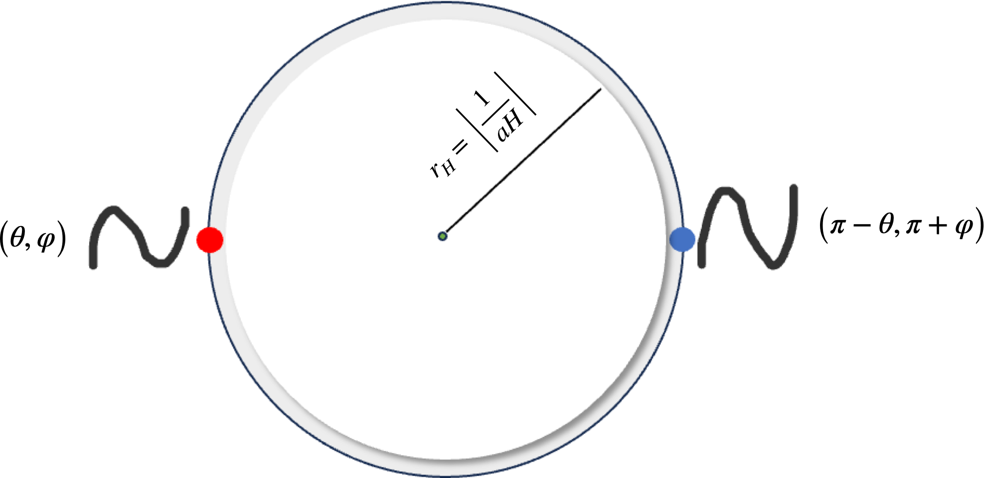
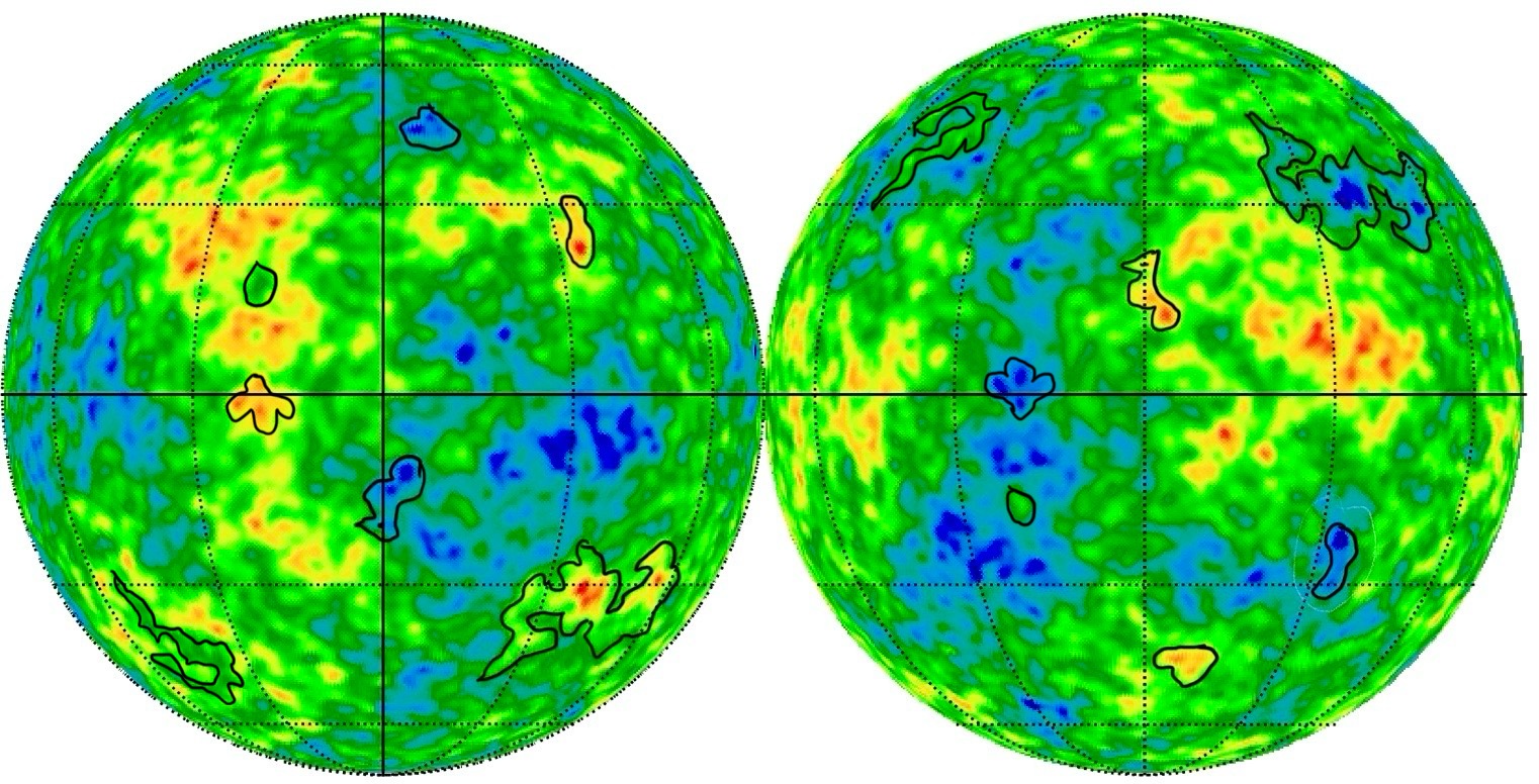
Figure 3: The top panel portrays the co-moving horizon during a particular moment of inflationary expansion, showcasing the evolution of a quantum fluctuation in DSI. This quantum fluctuation moves forward in time at $\left(\pi-\theta,\pi+\varphi\right)$ and backward at $\left(\theta,\varphi\right)$, leading to an odd parity excess due to the breaking of time-reversal symmetry by the background inflationary spacetime. In the bottom panel, you get a glimpse of the spherical distribution of the odd component in one such quantum fluctuation, displayed in two spherical caps centered at the red and blue points. The image is sourced from the odd component of the Planck 2018 (SMICA) map, which dominates over the even one (see also Fig. 9 and Fig. 18). We can schematically see here how quantum fluctuations in DSI can leave their imprints in the CMB once they exit the horizon and become super-horizon fluctuations.

The detailed explanation of the DSI theory is provided in Sec. 7. The primary and noteworthy new result presented in this paper is the even-odd asymmetric angular power spectrum:

$$C_{\ell}^{odd}=\frac{2}{9\pi}\int_{0}^{k_{c}}\frac{dk}{k}j_{\ell}^{2}\left(\frac{k}{k_{s}}\right){\mathcal{P}}_{\zeta}(k)\left(1+\Delta{\mathcal{P}}_{v}\right)$$ (17)

$$C_{\ell}^{even}=\frac{2}{9\pi}\int_{0}^{k_{c}}\frac{dk}{k}j_{\ell}^{2}\left(\frac{k}{k_{s}}\right){\mathcal{P}}_{\zeta}(k)\left(1-\Delta{\mathcal{P}}_{v}\right)$$

It’s essential to emphasize that this outcome introduces no new free parameters (with respect to the SI model in Eq.16) and simply emerges from:

$$\Delta{\mathcal{P}}_{v}=\left(1-n_{s}\right)\operatorname{Re}\left[\frac{1}{H_{3/2}^{(1)}\left(\frac{k}{k_{\ast}}\right)}\frac{\partial H^{(1)}_{\nu_{s}}\left(\frac{k}{k_{\ast}}\right)}{\partial\nu_{s}}\Bigg{|}_{\nu_{s}=\frac{3}{2}}\right]$$ (18)

Here, $H^{(1)}_{\nu_{s}}\left(z\right),j_{\ell}\left(z\right)$ is the Hankel and Bessel functions of first kind and $k_{c}=0.02k_{\ast}$ is the cut-scale we impose as (18) is accurate enough for low-$\ell$ or large angular scales (See Sec. (7) for more details). In the later sections, using (17) we compute several observables related to parity asymmetric CMB temperature maps at low-$\ell$ and compare them with the predictions of SI.

4 Standard inflation versus Direct-Sum inflation

In this section, the goal is to find out how probable DSI and SI are consistent with the parity asymmetric CMB data and vice versa.

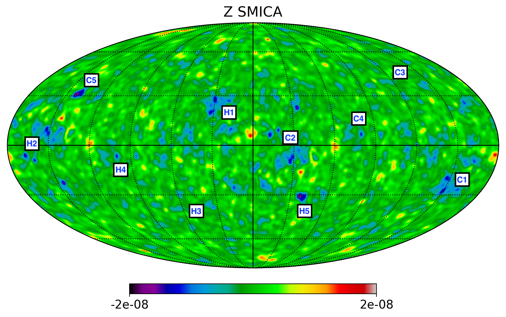
Figure 4: Un-normalised (units of Kelvin²) parity product: $Z(\hat{n})={\mathcal{T}}(\hat{n}){\mathcal{T}}(-\hat{n})$ for Planck (SMICA) map. This map is also a ${\mathcal{P}}$ conjugate image of itself. Positive values (red) correspond to the symmetric (even parity) component of ${\mathcal{T}}$ and negative values (blue) to the antisymmetric (odd parity) component. The $Z(\hat{n})$ map shows some extreme antisymmetric (i.e. blue) values that we already identified in the middle panel of Fig. 2 (we use the same labels here). But if we focus on values around the mean (i.e. cyan-blue and yellow-orange) there is an excess of negative $Z$ values, indicating a preference for odd parity. We will quantify this here by comparing the 1-point $P(Z)$ distributions in data and simulations.

We evaluate here the significance of the observed parity asymmetry by comparing the $Z$ parity 1-point $P(Z)$ distribution in the Planck maps with the corresponding distribution obtained from simulations of each model. The data and the simulated maps are processed in the same way (See Figs. 4, 20 and 21). More details on the simulations and their validation are given in Appendix C. Here we test two different theories of inflationary quantum fluctuations SI and DSI.

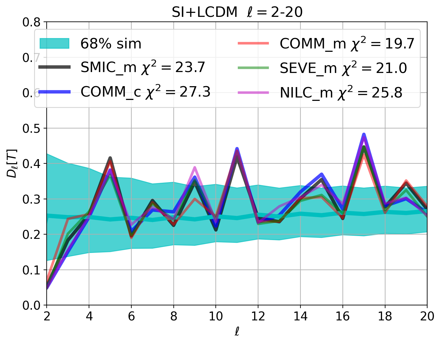
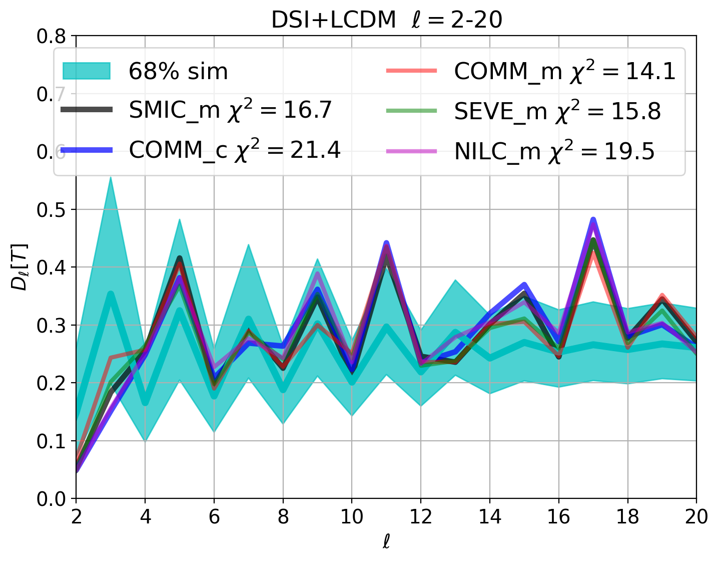
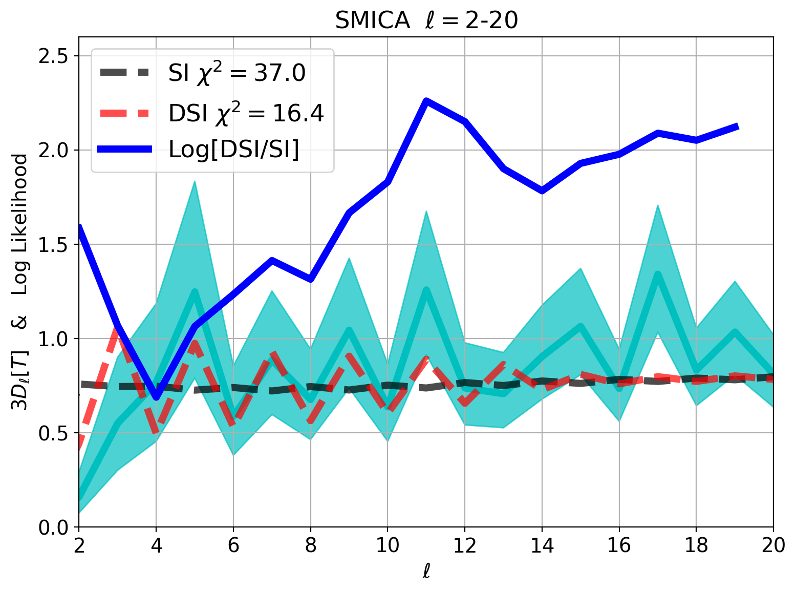
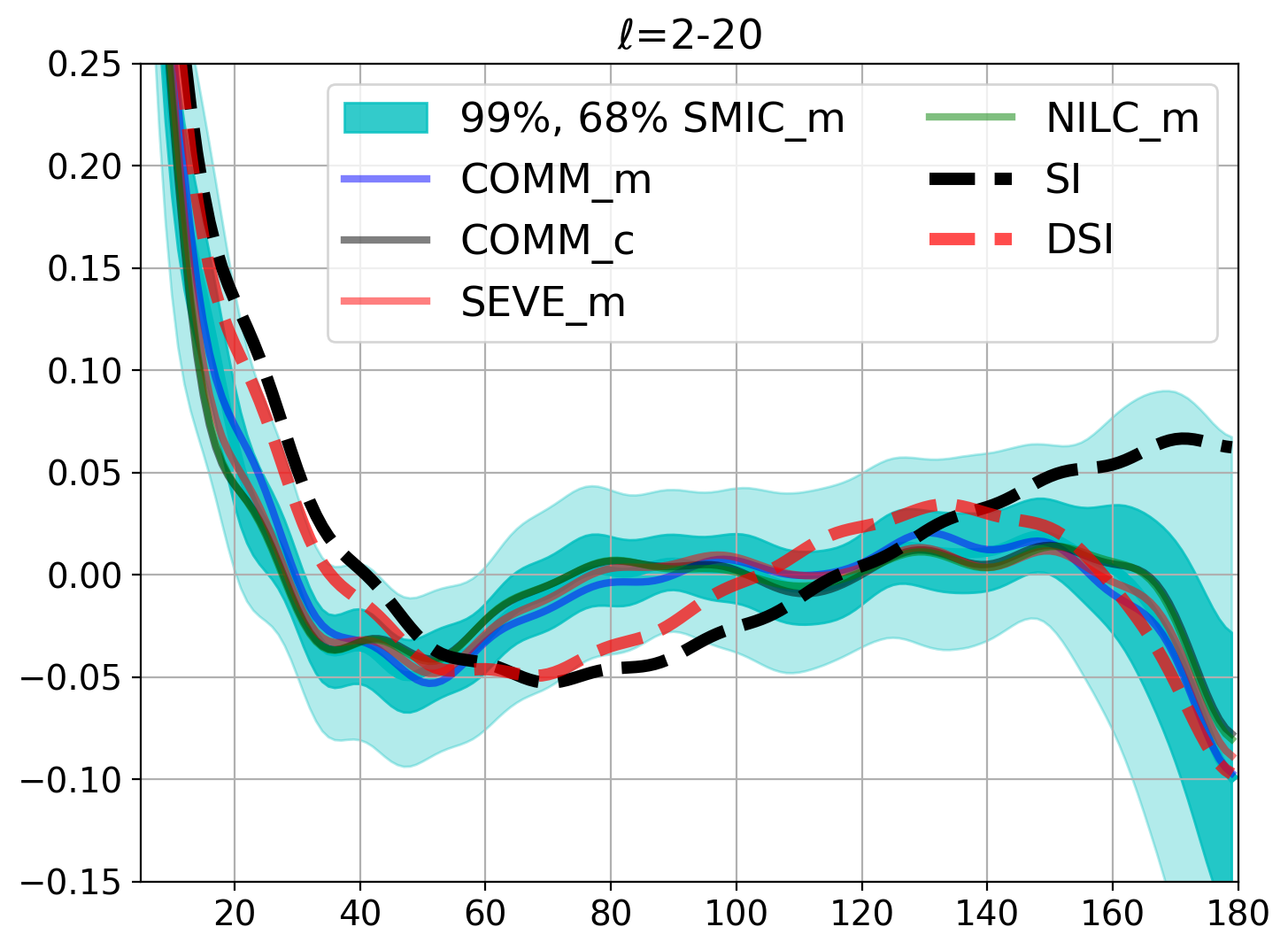
Figure 5: Comparison of measured $C_{\ell}$ in several Planck (masked, smoothed and normalized) temperature maps (lines labeled SMIC_m, COMM_m, COMM_c, SEVE_m and NILC_m) against the corresponding $C_{\ell}$ in different simulations (shaded regions correspond to 68% variations in the $10^{6}$ realizations). The top panels show simulations of SI (left) and DSI (right) LCDM models. The bottom left panel shows instead realizations of the observed Planck SMIC_m map compared to the same models. The blue line shows the log of the ratio of the cumulative DSI to SI likelihoods according to SMICA_m realizations: DSI is up to 150 times more likely than SI. The bottom right panel compares the corresponding $w(\theta)$ with 68% and 99% errors in the SMIC_m data, which it is also aligned with odd symmetry (compare to Fig. 9).

Fig. 5 shows a comparison of the normalized $C_{\ell}$ in the SI and DSI models against the corresponding outputs in the different Planck maps. Given our focus on the largest possible scales, our analysis is dominated by sampling variance, rendering other sources of errors and uncertainties negligible. Sampling variance errors are proportionate to the signal. Consequently, the errors depend on the assumptions we make regarding the model. We explore two distinct approaches. The first involves calculating errors from different models and estimating $p[D|M]$, the probability of the data $D$ given the model $M$. The top panels of Fig. 5 are examples of this. According to the $\chi^{2}$ test, the SMIC_m data in the range $\ell=2-20$ is closer to the DSI models (top right) than the SI model (top left), with a significance of $\Delta\chi^{2}\simeq 7$. Similar results are obtained for $\ell=2-30$, as shown in the bottom panels of Fig. 16.

In the second approach, we estimate errors in the data, by using the $C_{\ell}$ in the data as input for simulations. In this case, we estimate $p[M|D]$, the probability of the model given the data. The bottom left panel illustrates this second approach. The odd parity DSI model is also preferred, given the data, over standard LCDM (SI), but with a larger significance: $\Delta\chi^{2}=20.6$. This appears to indicate strong evidence for odd parity; however, as explained in Appendix B, it is not straightforward to convert such $\chi^{2}$ values into probabilities because, among other things, the $C_{\ell}$ distribution is not Gaussian for the lowest $\ell$. This is illustrated in the left panel of Fig. 14.

But we can directly estimate the likelihood ratio between DSI and SI using the data simulations, eliminating the need to presume a Gaussian distribution. We will still assume that the different $C_{\ell}$ values are approximately uncorrelated. This assumption seems reasonable, given that we have measured the covariance matrix and found that the Pearson cross-correlation coefficients are consistently smaller than 15% (see right panel of Fig. 14) and have little impact ($<15\%$) on the likelihood ratio.

In this scenario, the likelihood simplifies to the product of individual $C_{\ell}$ likelihoods. The blue line in the bottom left panel of Fig. 5 shows the logarithm of the ratio of cumulative likelihoods for the two models. Examining individual multipoles, the quadrupole $C_{2}$ alone indicates that DSI is about 40 times more likely than SI. However, when including $C_{3}$ and $C_{4}$, this ratio decreases below 10. Subsequent multipoles then elevate the accumulated likelihood ratio to over 100 at $\ell\simeq 11$. Based solely on the $C_{\ell}$ measurements, we can confidently assert that DSI is approximately 150 times more likely than SI (using $\ell<20$ or $\ell<30$). This substantial difference will be subjected to further testing using alternative approaches that focus solely on the measurements of parity.

The bottom right panel of Fig. 5 shows 68% and 99% confidence regions in the 2-point correlation $w(\theta)$ of the SMIC_m data realizations as compared to the DSI and SI mean model predictions using Eq. 8. Even when there is a lot of covariance in these measurements, the data is at odds with SI data in a very significant way (e.g. see text around Eq.106 and Camacho-Quevedo:2021bvt and references therein). As we will show, odd parity is very related to this anomaly both because it predicts a low $C_{2}$, which has a large impact on $w(\theta)$ (see Fig. 9), and also because of the strong observed negative correlation at $\theta=180^{\circ}$, connecting the antipodes at $\theta=180^{\circ}$ to $\theta=0^{\circ}$ with odd parity.

4.1 Results on parity asymmetry in SI versus DSI

We next present two alternative tests to compare models to data. The first one is based on configuration space, by doing a $\chi^{2}$ comparison of the full $P(Z)$ parity distribution. The second one shows a more direct comparison of the likelihood using extreme probabilities (p-values) of $R^{TT}$ in (14) and the quadrupole $C_{2}$ (i.e. in harmonic space) as well as moments (mean $Z^{1}$ and skewness $Z^{3}$) of the $P(Z)$ distribution (in configuration space).

4.1.1 Z-parity statistics

Fig. 4 shows a comparison of the $Z$ parity 1-point probability density distribution $P(Z)$, i.e. the probability for a given value of $Z$ to be observed, in models and observations (see also $Z$ maps in Fig. 6 and Fig. 18-21). The figures indicate a preference for odd parity in the measured CMB data. This pattern holds across various component separations and masking conditions (as labeled in the Figure). Notably, there is an excess of negative $Z$ values and a deficiency of positive ones compared to SI, which inherently lacks a defined parity. The DSI model, characterized by 20% excess in odd parity, appears to offer a much-improved fit to the data. Yet, how much improvement does it provide? The considerable covariance $C_{ij}$ between bins in the $P(Z)$ histogram (as illustrated in the lower right panel of Fig. 6) prompts the question of whether the observed differences are statistically significant. The $C_{ij}$ matrix shows 30-40% anticorrelation between the antipodal fluctuations in $Z$ and some 20-70% correlation within $Z$ fluctuations of the equal sign. This could, in principle, explain the observed parity asymmetry just as sampling variance fluctuations.

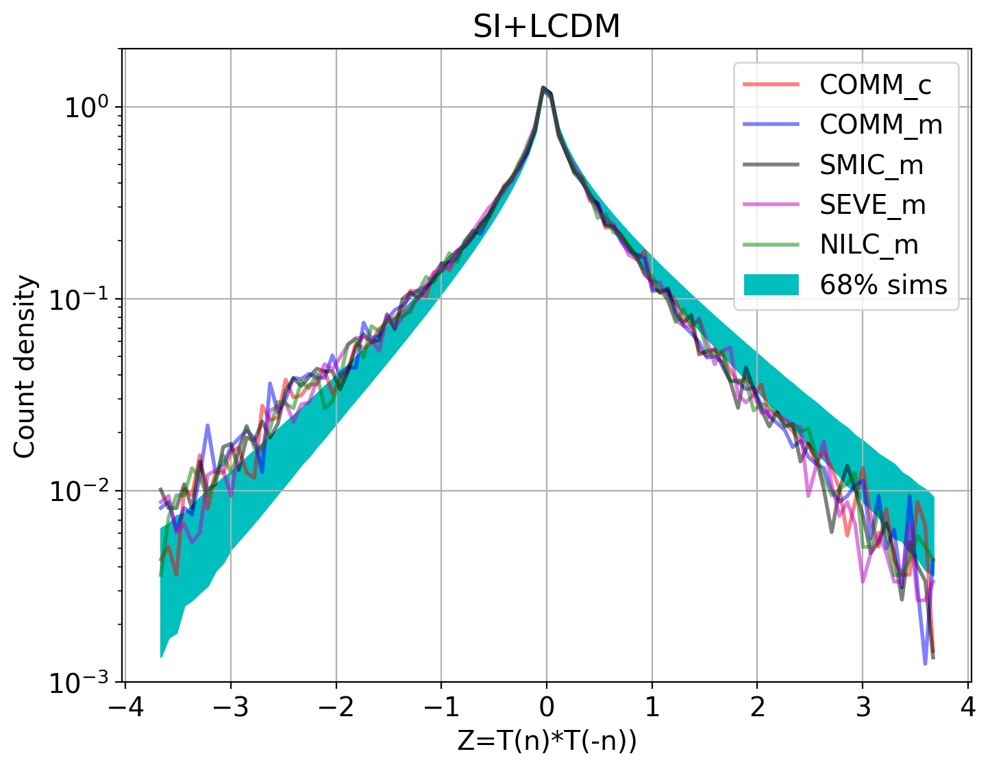
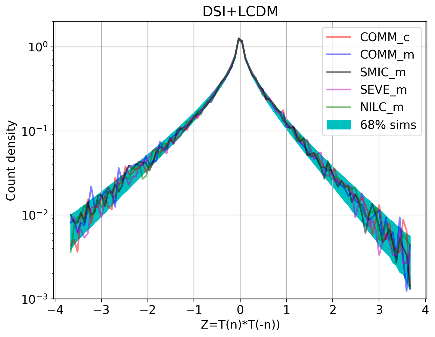
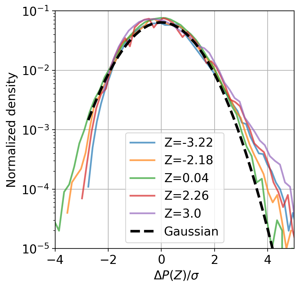
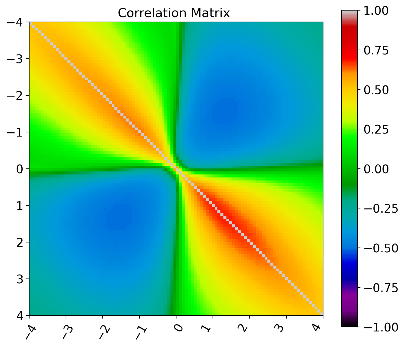
Figure 6: Top panels show $P(Z)$ histogram of $Z(\hat{n})\equiv{\mathcal{T}}(\hat{n}){\mathcal{T}}(-\hat{n})$ CMB maps (for the different component separation and masking) as compared with the corresponding $P(Z)$ in simulations of the best-fit LCDM with SI (left) or DSI (right). The shaded region corresponds to the 68% interval around the median in the corresponding simulations. There is an excess of negative $Z$ values in comparison with the lack of positive ones in the SI predictions, which indicates a preference for odd parity, in agreement with DSI. Bottom Left shows the distribution of normalized count variations $\hat{\Delta}_{i}$ in (19). This distribution is not well approximated by a Gaussian (dashed line) which makes it hard to interpret the $\chi^{2}$ test. Bottom Right shows the covariance in $P(Z)$, which is very similar for the different models.

To evaluate this, we perform a $\chi^{2}=\Delta_{i}C_{ij}^{-1}\Delta_{j}$ test on the histogram $P_{i}=P(Z_{i})$ presented in the top panels of Fig. 6. Here, $\Delta_{i}\simeq[P^{data}_{i}-P^{model}_{i}]/\sigma_{i}$ represents the normalized differences between the model realizations and data at bin $i$, and $\sigma_{i}$ denotes the RMS scatter in the realizations. We employed $10^{6}$ realizations for each model to calculate the normalized covariance matrix as:

$$C_{ij}\equiv<\hat{\Delta}_{i}\hat{\Delta}_{j}>\quad;\quad\hat{\Delta}_{i}\equiv\frac{P_{i}^{sim}-<P_{i}^{sim}>}{\sigma_{i}}.$$ (19)

In the expression above, $\hat{\Delta}_{i}$ represents the fluctuations in the simulations. The right bottom panel of Fig. 6 displays $C_{ij}$ for the SI realizations, with the covariance for DSI being very similar. The inversion of the covariance matrix $C_{ij}$ is performed using the (Moore-Penrose) pseudo-inverse based on Singular-Value Decomposition (SVD).

We obtained $\chi^{2}=109$ for SI and $\chi^{2}=97$ for DSI, considering 97 independent degrees of freedom after SVD. The data exhibits good agreement with the odd parity level in the DSI simulations. The larger value ($\Delta\chi^{2}\simeq 12$) for SI could in principle be interpreted as a $\sqrt{12}\sigma\simeq 3.5\sigma$ significant deviation. But as it happened for $C_{\ell}$, this result should be taken with some caution. The histogram of $\hat{\Delta}_{i}$ values deviates from a Gaussian distribution, especially noticeable for larger values of $Z$. This non-Gaussian behavior is explicitly depicted in the bottom left panel of Fig. 6 across various bins $i$ corresponding to different $Z$ values. Such deviations make it challenging to interpret the $\chi^{2}$ test accurately for model evaluation.

A more reliable approach is to directly assess the likelihood using p-values, similar to what was done for $C_{\ell}$ (See Appendix. B, as elaborated in the next section.

4.1.2 p-values

For a direct combination with the parity measurements in harmonic space, we will focus next on the mean and skewness of the $P(Z)$ distribution, which we call $Z^{1}\equiv\sum_{i}P_{i}Z_{i}$ and $Z^{3}\equiv\sum_{i}P_{i}Z_{i}^{3}$. These moments are not as constraining as the full parity $P(Z)$ distribution, but they are more easily cast in terms of p-values. We compute the p-value by determining the fraction of data simulations with $Z^{1}$ and/or $Z^{3}$ values more extreme than each model’s predictions. It’s important to note that because of the way the p-values are defined, they are constrained to be smaller than 50%.

The results are presented in Table. 1, where we also include the corresponding p-values (representing the probabilities of the model given the data: $p[M|D]$) for parity asymmetry in the quadrupole $C_{2}$ and the harmonic space even-odd ratio $R^{TT}$ in (14). Using the same $10^{6}$ data simulations for each case enables us to combine them, as illustrated in Fig. 7.

Table 1: Parity probability $p[M|D]$ ($\times 10^{2}$) of a model given the data (based on $10^{6}$ sky realizations of the data). Each CMB parity estimate (lines) is compared with the two different models: Standard Inflation quantum fluctuations with LCDM (SI) and direct-sum inflationary quantum fluctuations (DSI). Data is estimated from the Planck 2018 masked SMICA component separation map. Very similar results are found for the other maps (e.g. see Fig. 7). In the last column ’ratio’ refers to the ratio of probabilities between the DSI and SI predictions.

p-value: $p[M|D]\times 10^{2}$	SI	DSI	ratio
Harmonic space:			DSI/SI
$C_{2}$	0.09	3.3	37
$R^{TT}$ ($\ell\leq 20$)	0.7	39.5	56
$C_{2},R^{TT}(\ell\leq 20)$	0.003	1.96	653
Configuration space:
$Z^{1}=w[\pi]$	1.12	45.3	40
$Z^{3}$	2.10	45.6	22
$Z^{1},Z^{3}$	0.67	36.3	54
Combined:
$Z^{1},R^{TT}(\ell\leq 20)$	0.45	34.6	77
$Z^{1},C_{2}$	0.016	2.65	166

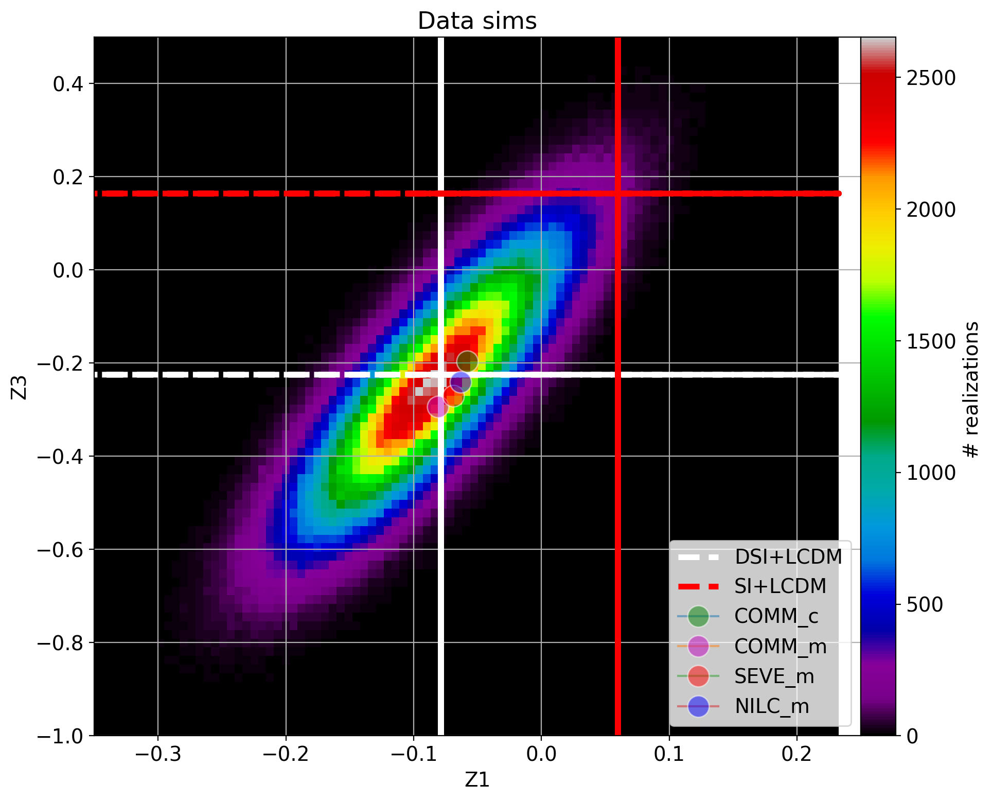
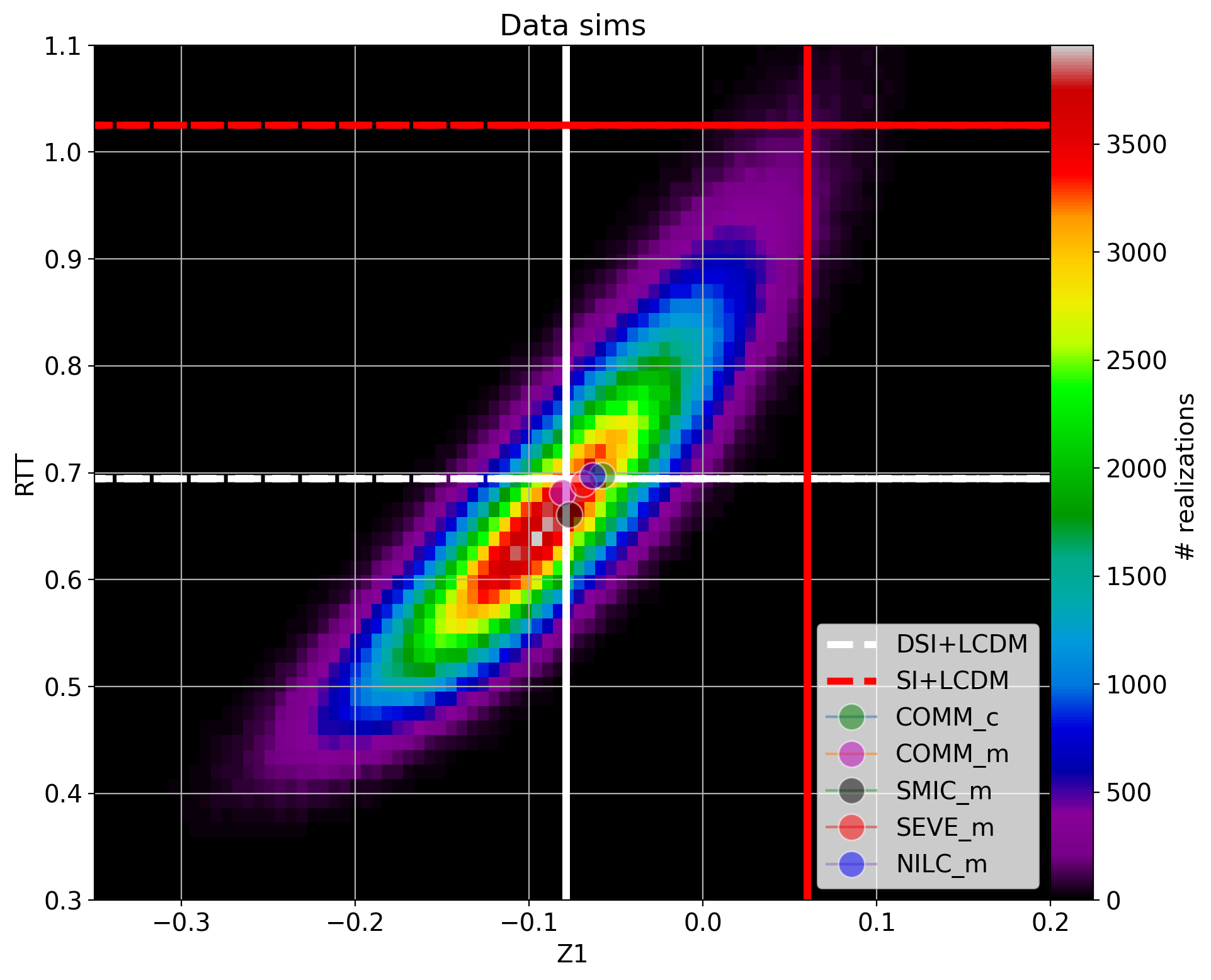
Figure 7: Colored points show the density of parity measurements in data (with sampling variance errors from $10^{6}$ realizations) as compared to the corresponding expected values in 2 different models (horizontal and vertical lines): SI (red) and DSI (white). The left panel shows the skewness $Z^{3}$ and mean $Z^{1}=w(\pi)$ of the $P(Z)$ parity distribution (i.e. parity in configuration space). The right panel shows $R^{TT}$ in (14) (i.e. parity in harmonic space) versus the mean $Z^{1}$. We also show the data measurements for different CMB Planck component separation methods (circles). The external boundaries of the yellow, blue, and magenta points correspond to 1, 2, and 3$\sigma$ confidence levels (see also Fig. 8).

Fig. 8 shows the other combinations presented in Table 1. The model predictions for SI (red) and DSI (blue) are shown as vertical and horizontal lines in Fig. 8. The data prefers DSI over SI with a significance of more than $3\sigma$, in good agreement with the direct $P(Z)$ test (shown in Fig. 6) or the p-values in Table. 1. In particular, SI is ruled out at more than $3\sigma$ in any combination involving $C_{2}$, while DSI can explain the $C_{2}$ and all other parity measurements within $2\sigma$ confidence interval.

Table 2: Probability ($\times 10^{2}$) $p[D|M]$ of the data being more extreme than a model realization (based on $10^{6}$ masked sky simulations of the model). Each CMB anomaly (lines) is compared with 2 different models (columns): Standard Inflation quantum fluctuations with LCDM (SI+LCDM) and direct-sum inflationary quantum fluctuations (DSI+LCDM). Data is estimated from the Planck 2018 masked SMICA component separation map. Very similar results are found for the other maps (e.g. see Fig. 7). In the last column ’ratio’ refers to the ratio between the DSI and SI predictions.

p-value: $p[D|M]\times 10^{2}$	SI	DSI	ratio
Parity:			DSI/SI
$C_{2}$	2.62	8.88	3.4
$R^{TT}$ ($\ell\leq 20$)	1.00	39.7	40
$Z^{1}=w[\pi]$	3.89	46.3	12
$Z^{3}$	1.78	37.1	21
$Z^{3},R^{TT}$	0.58	32	55
$C_{2},R^{TT}$	0.12	5.59	47

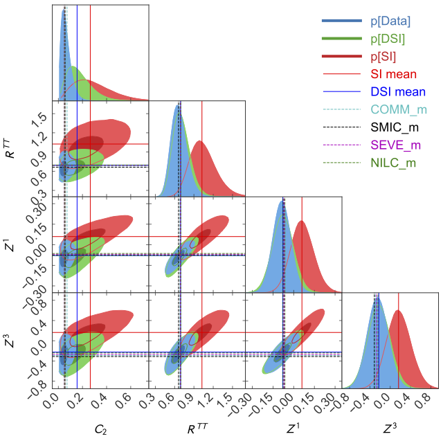
Figure 8: Similar to Fig. 7, this shows parity measurements for 4 different Planck component separation maps and masking methods (dashed lines) compared to contours of cosmic variance uncertainties (from $10^{6}$ realizations each) of the data (blue), SI (red) and DSI (green) models. The shaded regions correspond to 1 and 2-sigma confidence levels in the simulations. Note that the errors are dominated by cosmic variance, which are included both in the data and in the models. We can either look at $P[D|M]$: i.e. where the mean data lies within the model realizations, or at $P[M|D]$: where the mean of the models lies within the data realizations. The latter is more constraining and well-defined. The mean DSI model is within the 1-2$\sigma$ data contours whereas SI is ruled out with more than 3$\sigma$ confidence (see also Table. 1).

The other Planck component separation maps plotted as circles in Fig. 7 or lines in Fig. 8, are close to SMIC_m and the small differences can mostly be attributed to the difference in the size of the masking areas. The DSI results exhibit close similarity to data. Given that both SI and DSI models share the same number of parameters (as dictated by the best LCDM fit used as $C_{\ell}$ input to the simulations), we can confidently assert that DSI is up to $\simeq 80-650$ times more probable than SI. This agrees well with the cumulative likelihood ratios based on the $C_{\ell}$ shown as a blue line in the bottom left panel of Fig. 5.

Table. 2 presents the corresponding probabilities based on model simulations (probabilities of the data given the model: $p[D|M]$), and the results agree qualitatively with Table 1. Generally, the latter provides more stringent constraints, as the sampling variance errors are smaller for realizations based on the data (due to the smaller $C_{2}$ value). The p-values obtained for SI in Table. 2 align with those found in previous literature (e.g., see Fig. 3 of Muir:2018hjv and references therein).

When $C_{2}$ is fixed in SI to match the data (model SI-$C_{2}$), the $P(Z)$ predictions get closer to observations. This makes sense because $C_{2}$ is the first and largest of the odd parity oscillations. However, additional evidence in favor of odd parity remains without $C_{2}$, as indicated by the comparison of p-values in the third columns of Table. 2 and Table. 3.

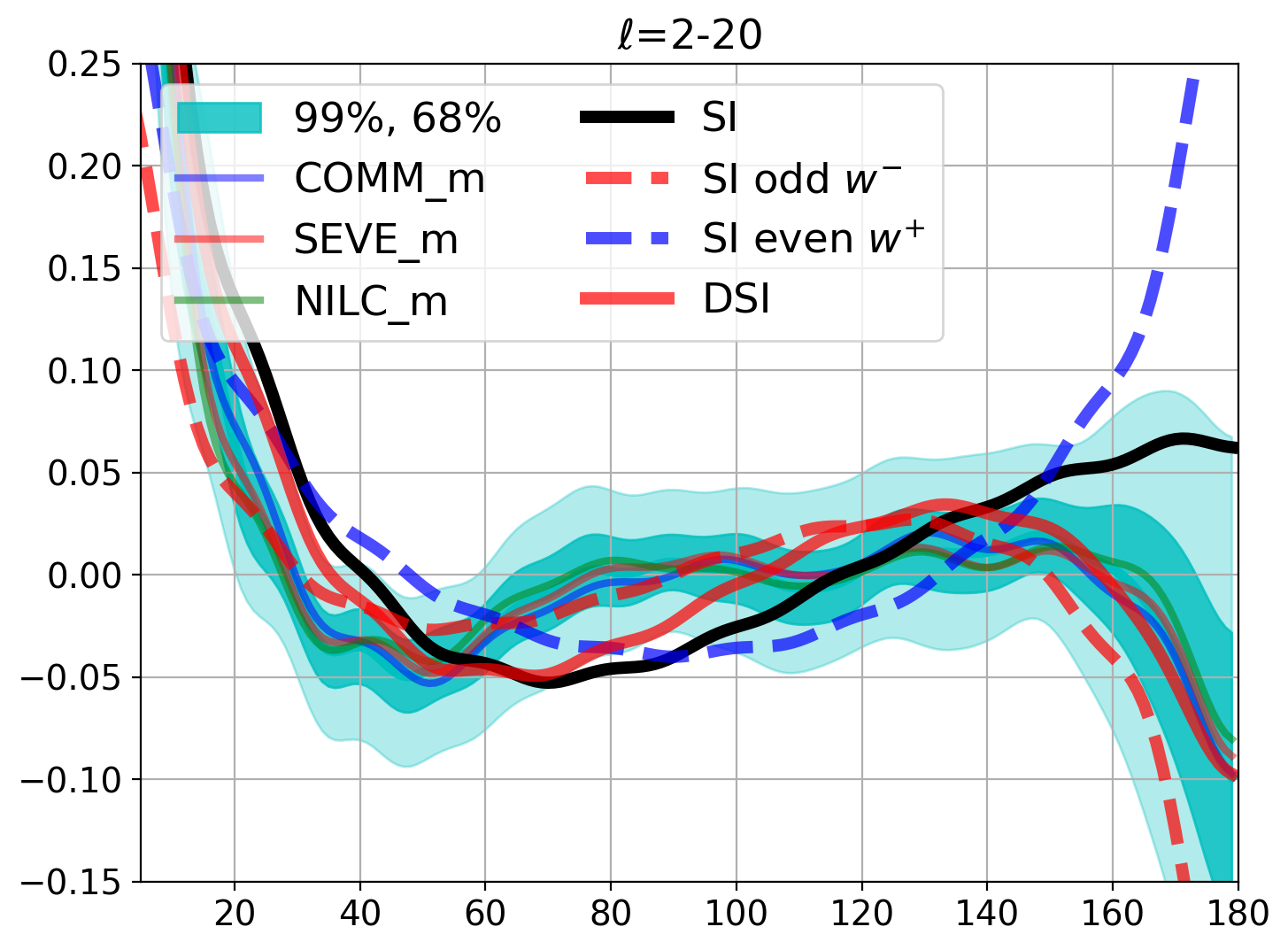
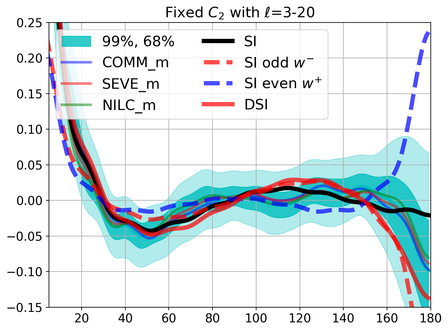
Figure 9: Comparison of the 2-pt temperature correlation $w(\theta)$ estimated from $C_{\ell}$ in (8) with $\ell_{max}=20$. Results for larger $\ell_{max}$ are the same for separations $\theta>8^{\circ}$. The 99% and 68% regions (cyan) allowed by the SMIC_m Planck map (with $10^{6}$ sampling realizations) are compared with the SI best-fit model ($w$, black) split into odd ($w^{-}$, red dashed) and even ($w^{+}$, blue dashed) parity contributions. The data is closer to the odd component. The right panel shows the result of replacing the quadrupole $C_{2}$ in the SI and DSI models with the one measured in the SMIC_m map (i.e. model SI-$C_{2}$ in Table. 3). This makes all the curves closer to the data and resolves the anomaly in $S_{1/2}$ (see (106) and Table. 3). But even with a low $C_{2}$ the data is more odd than the average SI model, with strong antisymmetry between antipodal angles.

5 Connection between lack of correlations at $\theta>60^{\circ}$ and lower quadrupole

From Tables. 1 and 2 we can read that the DSI model predicts lower quadrupole than with a high $p-$value in comparison with SI model. We can see in this in Figs. 5 and Fig. 8 as well. Another CMB anomaly other than parity is called $S_{1/2}$ and is related to the lack of angular correlations (8) at $\theta>60^{\circ}$ (See Appendix. D). Fig. 9 illustrates the decomposition of $w[\theta]$ in (8) into even (red) and odd (blue) parity contributions using the same $C_{\ell}$ values displayed in Fig. 5. The Planck map and simulations align more closely with the odd component of the SI model, in agreement with the odd-even oscillations in $C_{\ell}$ that we showed in Fig. 5. It’s remarkable to observe that the antisymmetric part of Fig. 9—depicted by the red dashed line, representing the odd component of temperature fluctuation in the SI model—successfully connects antipodes at $\theta\simeq 180^{\circ}$ to $\theta\simeq 0^{\circ}$ with comparable amplitudes but opposite signs. This alignment provides compelling evidence that the CMB sky is predominantly influenced by the odd component, confirming our visual observation in Fig. 2. Thus, observations not only imply homogeneity (due to the absence of anisotropies on the largest scales: $\theta>60^{\circ}$ or $\ell<4$) but also reveal an excess of odd parity (evidenced by the equal amount of negative and positive correlations at the largest and smallest scales). Despite the potential impact of the mask on the $C_{\ell}$ measurements, a direct estimation of $w(\theta)$ in configuration space yields results very similar to the straightforward sum of $C_{\ell}$ in harmonic space presented here (see, for instance, gazta2003 ; Camacho-Quevedo:2021bvt ). From the right panel of Fig. 9, where the SI+LCDM model fixes the value of the quadrupole $C_{2}$ to align with CMB data measurement, we can infer that this model better accounts for the absence of correlations at $\theta>60^{\circ}$. However, SI+LCDM still falls short in addressing the observed anticorrelation at $\theta=180^{\circ}$, a challenge effectively met by the DSI model. Considering that the likelihood of DSI explaining the quadrupole is 37 times higher than SI (see Table. 1), it becomes evident that DSI not only accounts for the observed lack of correlations at large angular scales but also captures the antipodal odd symmetry.

We have quantified the anomaly in $S_{1/2}$ in (106) and presented the corresponding p-values in Table. 3. The obtained p-values are notably low, aligning with previous findings (see, for instance, Muir:2018hjv ; Jones:2023ncn and references therein, and also Camacho-Quevedo:2021bvt for a related study). As demonstrated in the second column of Table. 3, the low p-value is primarily a consequence of the reduced quadrupole $C_{2}$ in the data. When we hold $C_{2}$ fixed at the observed value (in SMIC_m), the probability increases by a factor of 122. This shift is visually represented in Fig. 9.

6 Revising HPA with de-biased simulations and lower-quadrupole

Table 3: Probability ($\times 10^{2}$) $p[D|M]$ of the data being more extreme than a test model realization (based on $10^{6}$ masked sky simulations of the model). Each CMB anomaly (lines) is compared with 2 different test models (columns) against Standard Inflation with LCDM (SI+LCDM): The second column is SI+LCDM but with quadrupole $C_{2}$ being fixed to data (SI-$C_{2}$), anisotropic dipolar modulation (DPM with $A=0.07$ or $A=0.5$). Data is estimated from the Planck 2018 masked SMICA component separation map. Very similar results are found for the other maps (e.g. see Fig. 7-Fig. 8). In the bottom of the Table we show other anomalies of the SI+LCDM model, which are in principle not directly related to Parity. These anomalies vanish for the low $C_{2}$ version of the model.

p-value: $p[D|M]\times 10^{2}$	SI	SI-$C_{2}$	DPM
Parity:			A=0.07 (0.5)
$C_{2}$	2.62	47.8	2.6 (2.1)
$R^{TT}$ ($\ell\leq 20$)	1.00	4.07	1.0 (0.4)
$Z^{1}=w[\pi]$	3.89	19.3	4.0 (3.9)
$Z^{3}$	1.78	9.0	1.8 (1.8)
$Z^{3},R^{TT}$	0.58	3.01	0.7 (0.3)
$C_{2},R^{TT}$	0.12	1.31	0.1 (0.03)
Other Anomalies:
2-pt $w(\theta)$: $S_{1/2}$	0.08	9.8
HPA: $\sigma^{2}_{16}$	0.49	4.6
HPA: $\sigma^{2}_{16}[db]$	2.50	14.9

In this section, we revisit one of the most explored CMB anomaly called Hemispherical Power Asymmetry (HPA) which implies CMB in a preferred direction has a maximal power asymmetry. Visually you can see this annomaly in the top right panel of Fig.15 which shows the Planck map with a low resolution in Ecliptic coordinates. In those coordinates, the amplitude of fluctuations are clearly larger in the South than in the North Ecliptic cap. As a result there is an alignment of the $C_{2}$ and $C_{3}$ multipoles with the Ecliptic plane. This can be modeled as a dipolar modulation (DPM) and the empirical fit to the CMB data has been found to be the following Akrami:2014eta

$$T(\hat{n})=\left(1+A\,\hat{n}.\hat{m}\right)\,T_{iso}(\hat{n}),$$ (20)

where $T_{iso}$ will be model as the SI+LCDM model with an isotropic spectrum of fluctuations and $\hat{m}$ is a fixed direction in the sky (the origin of the anisotropy). $A\simeq 0.07$ is the amplitude of anisotropies that is consistent with the maximum measured HPA asymmetry in Planck data Namjoo:2014nra . The HPA was also claimed to be the feature in WMAP analysis Hansen:2008ym which has triggered numerous theoretical studies (See Erickcek:2008jp ; Erickcek:2008sm and the cited of them). The appearance of HPA in the particular direction of ecliptic coordinates (i.e., the direction of the orientation of the solar system) is coined to be the axis of evil, and even some late-time observations have supported it Land:2005ad ; Secrest:2020has . Recently this has gained much more attention in the form of conclusive evidence for the violation of isotropy or cosmological principle Jones:2023ncn ; Aluri:2022hzs . First of all, this finding if true does change our understanding of cosmology but it is important to carefully scrutinize the finding even further which is what we aimed to do in this section. Notably, in Quartin:2014yaa a critical analysis of HPA was performed and it was concluded to be insignificant. We also reach a similar conclusion in our analysis with our direction-de-biased simulations of HPA which will be explained shortly. In all the previous sections, our focus was only on parity, now we can ask a much more generic question which is if HPA advocated by the relation (20) has anything to do with Parity. The value of $A\approx 0.07$ has very little impact in our parity test and we will therefore also try an extreme case of $A=0.5$. Another question we can ask is whether DPM or HPA can be originated from low-quadrupole $C_{2}$?

As shown in the 3rd column of Table. 3, the anisotropic DPM model yields very similar parity results to the SI+LCDM model, even when we increase the asymmetry in (20) to an extreme dipole with $A=0.5$. The case of $A=0.5$ is illustrated in the bottom right panel of Fig. 15 (in Ecliptic coordinates) and in Fig. 22 (in Galactic coordinates). We found that even such a substantial anisotropy proves insufficient to account for the observed parity asymmetry, particularly in the $R^{TT}$ or $P(Z)$ measurements.

This occurs because the anisotropy is generated in a single fixed direction in each simulation to match the corresponding anisotropy found in the data. In that direction, the $Z$ values will have a negative background contribution between antipodal points, akin to the odd-parity case. However, because we average over all directions, this has a minimal impact on the overall $P(Z)$ statistics. The $P(Z)$ distribution for DPM is very similar to that of the SI simulations in Fig. 6. In terms of $C_{\ell}$, regardless of how large $A$ is, there is no alteration to the odd-even oscillations ($R^{TT}$) of each isotropic (LCDM) realization. Consequently, parity remains unaffected. These findings are also evident from the examination of Table. 2-3 and underscore the fundamental distinctions between parity and anisotropies. Parity cannot be altered by anisotropies. Isotropy constitutes a rotational symmetry, whereas parity is a separate discrete symmetry that is superimposed on top.

Additionally, we’ve calculated the Hemispherical Power Asymmetry (HPA), characterized by the low variance $\sigma_{16}^{2}=<\Delta T^{2}>$ in the North ecliptic sky, employing a resolution of $N_{nside}=16$ and $r_{beam}=10.5^{\circ}$, as defined in Muir:2018hjv (refer to our Fig. 15). The corresponding p-values for each test are shown in the bottom entries of Table. 2.

The $\sigma_{16}^{2}$ value in the Planck 2018 data reflects the outcome of a directional search to find the hemisphere in which $\sigma_{16}^{2}$ is lower for a specific direction. Such a search found it to be near the North ecliptic hemisphere. However, in the simulations, the $\sigma_{16}^{2}$ value is derived from a single direction in each realization of SI+LCDM (which is random for isotropic Gaussian fluctuations). This discrepancy introduces a substantial bias in the p-values, as we are comparing different statistics in data and simulations. To rectify this bias, we conduct the test $\sigma_{16}^{2}[db]$ (de-bias value) by searching for the smallest $\sigma_{16}^{2}$ in $10^{3}$ directions in each of the $10^{6}$ realizations for each model, mirroring the approach done with the data. In both SI and DSI models, the p-value for $\sigma_{16}^{2}[db]$ is approximately 5 times larger than in $\sigma_{16}^{2}$.

These anomalies are not inherently linked to parity asymmetry. However, their statistics are influenced by the parity in the data, as evidenced by the comparison between SI and SI-$C_{2}$ in the lower entries of Table. 2. When $C_{2}$ is low, the significance of the HPA or DPM-related anomalies largely disappear. We can therefore interpret all these anomalies as resulting from the odd parity in the data, which explains the low $C_{2}$ (with a p-value of approximately 9% in Table. 2 and a p-value about 40 times larger than SI in Table. 1), without the necessity of breaking isotropy or a deviation from the primordial scale-invariant spectrum.

It is intriguing how $P(Z)$ and the other CMB anomalies at large scales, while potentially explained by odd parity asymmetry, still leave room for more profound deviations. DSI provides an over 100 times better explanation of the CMB data than SI, yet it still has a low p-value for the combination of $C_{2}$ with several parity measures (i.e. $R^{TT}$ or $Z^{1}$) in Table. 1. The notion that the cosmological constant $\Lambda$ might play the role of a cosmic boundary condition opens up fascinating possibilities Gaztanaga2021 ; Gaztanaga2022 ; BHU1 ; BHU2 ; gaztanaga2023b . It aligns well with this and other observations that indicate a bounded (or finite) universe Fosalba:2021 ; Gaztanaga:2022bdh ; gaztanaga2023a .

7 Inflationary quantum fluctuations with direct-sum QFT

In this section, we discuss the formulation of DSI through the direct-sum quantum field theory (DQFT) in curved spacetime proposed in Kumar:2022zff ; Kumar:2023ctp ; Kumar:2023hbj .

Before we delve into DSI, we first start with a review of the theory of quantum fluctuations in SI. Then, we pull out the fundamental concerns of SI. Then lay out the theme of DSI emanating from the foundations of discrete spacetime transformations and their connection with the direct-sum construction of Hilbert/Fock space.

7.1 Reviewing Standard Primordial Inflation (SI)

Inflation by definition, is a quasi-de Sitter (qdS) expansion of the Universe that is expected to last around 50-60 e-folds before exiting to reheating phase where particle production happens and the Universe eventually enters into a radiation-dominated era Starobinsky:1981vz . To drive inflationary cosmic expansion we require at the minimum a new scalar degree of freedom which would result in a non-perturbative modification of GR whose action can be written as

$$S=\int d^{4}x\sqrt{-g}\left[\frac{1}{2}R-\frac{1}{2}(\partial_{\mu}\phi)(\partial^{\mu}\phi)-V\left(\phi\right)\right]\,,$$ (21)

where the potential $V(\phi)$ is essential and it require to have a plateau-like shape to explain the the current CMB contraints Planck:2018jri . The Starobinsky potential

$$V(\phi)=\frac{3}{4}M^{2}\left(1-e^{-\sqrt{\frac{2}{3}}\frac{\phi}{M_{p}}}\right)^{2}\,.$$ (22)

which is based on the quadratic scalar curvature modification of gravity is the most consistent theory with observations so far. Moreover, the Starobinsky-like inflationary scenarios are found to occur in multiple frameworks of quantum gravity that are currently the active field of research Koshelev:2017tvv ; Koshelev:2022olc ; Koshelev:2023elc ; Linde:2014nna ; Ellis:2013nxa . Even though inflationary quantum fluctuations are largely understood to be the origin of density fluctuations observed through the CMB, still there are fundamental questions related to the quantum effects in curved spacetime which we shall discuss in the next section. Before that, it is vital here to recall the minute details of SI quantum fluctuations Mukhanov:1990me .

The scalar perturbations arise from metric fluctuations ($g_{\mu\nu}=\bar{g}_{\mu\nu}+\delta g_{\mu\nu}$) and also the scalar field fluctuations ($\phi=\bar{\phi}+\delta\phi$). The metric fluctuations can be represented by the Arnowitt-Deser-Misner (ADM) metric of the form

$$ds^{2}=a^{2}\left(\tau\right)\Big{(}-{\mathcal{N}}^{2}d\tau^{2}+\gamma_{ij}\left(dx^{i}+{\mathcal{N}}^{i}d\tau\right)\left(dx^{j}+{\mathcal{N}}^{j}d\tau\right)\Big{)}\,.$$ (23)

where $d\tau=\frac{dt}{a}$ is conformal time, ${\mathcal{N}}$ and ${\mathcal{N}}_{i}$ are the lapse and shift functions respectively. In the unitary gauge, we fix $\delta\phi=0$ then we linearly expand the ADM metric as

$${\mathcal{N}}=1+\delta{\mathcal{N}},\quad{\mathcal{N}}_{i}=a\partial_{i}\chi,\quad\gamma_{ij}=\left(1+2\zeta\right)\delta_{ij}+h_{ij}\,,$$ (24)

where $\chi$ is a scalar function of spacetime, $\zeta$ is the curvature perturbation , $h_{ij}$ is the transverse and traceless spin-2 fluctuation. In this paper, we only focus on scalar flucutations as our study is only about temperature fluctuations in the CMB. From the linear perturbed equations of motion, we obtain the following constraints

$$\delta{\mathcal{N}} =\frac{\dot{\zeta}}{H}$$ (25)

$$\partial^{2}\chi =-\frac{\partial^{2}\zeta}{H}+\epsilon a^{2}\dot{\zeta}$$

Substituting (23) into the action (21) and expanding to second order in the fluctuations, we find the second order action for the scalar perturbation:

$$\delta^{(2)}S_{s}=\frac{1}{2}\int d\tau d^{3}xa^{2}\frac{\phi^{\prime 2}}{{\mathcal{H}}^{2}}\Bigg{[}\zeta^{\prime 2}-\left(\partial\zeta\right)^{2}\Bigg{]}\,\text{,}$$ (26)

where ${\mathcal{H}}=\frac{a^{\prime}}{a}=aH$ and $\tau=\int\frac{dt}{a}=-\frac{1}{aH}$ is the conformal time.

To quantize the scalar fluctuations we perform a field redefinition to define a canonical variable

$$v=a\zeta\dot{\phi}/H$$ (27)

given by

$$\delta^{(2)}S_{s}=\frac{1}{2}\int d\tau d^{3}x\Big{[}v^{\prime 2}-\left(\partial_{i}v\right)^{2}-\left(\frac{\nu_{s}^{2}-\frac{1}{4}}{\tau^{2}}\right)v^{2}\Big{]},$$ (28)

where $\nu_{s}$ is a function of the slow-roll parameters

$$\epsilon=-\frac{\dot{H}}{H^{2}},\quad\eta=\frac{\dot{\epsilon}}{H\epsilon}$$ (29)

as

$$\nu_{s}=\frac{3}{2}+2\epsilon+\eta\,.$$ (30)

7.2 Standard inflationary quantum fluctuations

By inspection, we can recognize that (28) $v$ is a Klein-Gordan field with time-dependent mass $m_{eff}^{2}=\frac{\nu_{s}^{2}-\frac{1}{4}}{\tau^{2}}$. Quantization means we promote the canonical variable to an operator and express it in terms of creation and annihilation operators as

$$\hat{v}\left(\tau,\,\textbf{x}\right)=\int\frac{d^{3}k}{\left(2\pi\right)^{3/2}}\Big{[}\hat{a}_{\textbf{k}}v_{k}\left(\tau\right)e^{i\textbf{k}\cdot x}+\hat{a}_{\textbf{k}}^{\dagger}v_{k}\left(\tau\right)e^{-i\textbf{k}\cdot x}\Big{]}\,.$$ (31)

The crux of quantum theory lies in the non-commutativity of the fields and its conjugate momenta that results in

$$\Big{[}\hat{v}\left(\tau,\,\textbf{x}\right),\,\hat{v}^{\prime}\left(\tau,\,\textbf{y}\right)\Big{]}=i\delta\left(\textbf{x}-\textbf{y}\right)$$ (32)

supplemented by

$$\Big{[}a_{\textbf{k}},\,a_{\textbf{p}}^{\dagger}\Big{]}=\delta\left(\textbf{k}-\textbf{p}\right)\quad\Big{[}a_{\textbf{k}},\,a_{\textbf{p}}\Big{]}=\delta\left(\textbf{k}-\textbf{p}\right)$$ (33)

The mode function $v_{k}$ satisfies the Mukhanov-Sasaki (MS) equation

$$v_{k}^{\prime\prime}+\left(k^{2}-\frac{\nu_{s}^{2}-\frac{1}{4}}{\tau^{2}}\right)v_{k}=0\,.$$ (34)

whose solution in the limit $\nu_{s}\to 3/2$ (i.e., neglecting slow-roll contributions since $\epsilon,\,\eta\ll 1$ during inflation) is given by

$$v_{k}(\tau) =A_{k}\frac{\sqrt{\pi|\tau|}}{2}H_{3/2}^{(1)}\left(-k\tau\right)+B_{k}\frac{\sqrt{\pi}|\tau|}{2}H_{3/2}^{(2)}\left(-k\tau\right)$$ (35)

$$=\frac{A_{k}}{\sqrt{2k}}e^{-ik\tau}\left(1-\frac{i}{k\tau}\right)+\frac{B_{k}}{\sqrt{2k}}e^{ik\tau}\left(1+\frac{i}{k\tau}\right)\,$$

where $A_{k}$ and $B_{k}$ are the Bogoliubov coefficients which can are in principle functions of $k$ satisfying the following constraint which is obtained by substituting (35) in (32)

$$|A_{k}|^{2}-|B_{k}|^{2}=1\implies\Big{\{}A=\cosh\alpha_{k},\,B_{k}=\sinh\alpha_{k}\Bigg{\}}\,.$$ (36)

From (35) we can learn that in the limit $|k\tau|\gg 1$ we end up with

$$v_{k}^{\rm{MS}}=v_{k}\Bigg{|}_{|k\tau|\gg 1}\approx\frac{A_{k}}{\sqrt{2k}}e^{-ik\tau}+\frac{B_{k}}{\sqrt{2k}}e^{ik\tau}$$ (37)

Considering $A_{k}=1$ and $B_{k}=0$ the mode function behaves as a positive energy state that is defined according to the Schrödinger equation

$$i\frac{\partial}{\partial t_{p}}|\Psi\rangle=\hat{H}|\Psi\rangle\implies\Psi_{t}=e^{-i\hat{H}t_{p}}|\Psi\rangle_{0}\,,$$ (38)

where $t_{p}$ is the parametric time of quantum mechanics and $\hat{H}$ is the time-independent Hamiltonian and $|\Psi\rangle$ state vector of Heisenberg representation. The vacuum

$$a_{\textbf{k}}|0\rangle_{\rm{BD}}=0\,.$$ (39)

corresponds to the choice $A=1$ and $B=0$ is also called the Bunch-Davies or adiabatic vacuum. The power spectrum of curvature perturbation is obtained by

$$P_{\zeta} =\frac{k^{3}}{2\pi^{2}a^{2}}\left(\frac{1}{\sqrt{2\epsilon}}\right)^{2}\Big{|}v_{k}\Big{|}^{2}\,$$ (40)

$$=\frac{H^{2}}{8\pi^{2}\epsilon}\left(1+\frac{k^{2}}{a^{2}H^{2}}\right)$$

where in the second line we substituted $\tau^{2}=\frac{1}{a^{2}H^{2}}$. For $k^{2}\ll a^{2}H^{2}$ the power spectrum just depends on background quantities $H,\,\epsilon$. Therefore, we can evaluate the power spectrum at a moment $k=aH$ by normalizing it with a factor of 2 for every mode that crosses the horizon Kinney:2009vz . Thus the (near) scale-invariant power spectrum is just given by the background quantities as

$$P_{\zeta}\approx\frac{H^{2}}{8\pi^{2}\epsilon}\,.$$ (41)

This power spectrum has a non-zero tilt because the background quantities $H,\,\epsilon$ are time-dependent and every time a mode exits the horizon $k=aH$ the value of the power spectrum is slightly changed by

$$n_{s}-1=\frac{d\ln P_{\zeta}}{d\ln k}\approx-\frac{d\ln P_{\zeta}}{dN}\approx-2\epsilon-\eta\,.$$ (42)

where $N$ is the number of e-foldings counted from the end of inflation. Combining (41) and (42) we get the near-scale invariant power spectrum in the well-known power-law form

$$P_{\zeta}\approx A_{s}\left(\frac{k}{k_{\ast}}\right)^{n_{s}-1}\,,$$ (43)

where $k_{\ast}=0.05\,{\rm Mpc}^{-1}$ at which $A_{s}=2.2\times 10^{-9}$ from the latest Planck data Planck:2018jri . The angular power spectrum of SI is computed following (103).

A caveat in the calculation of power spectrum (43) is that slow-roll corrections in the MS equation (34) are neglected by taking $\nu_{s}\approx\frac{3}{2}$. On the other hand, the full actual calculation including slow-roll corrections has to deal with applying approximations on the Hankel functions in the super-horizon limit and eventually estimating the quantities at Horizon exit Kinney:2009vz ; Powell:2006yg ; vennin:tel-01094199 . The approximate mode functions (35) are devoid of information related to slow-roll parameters and thus we do not capture correctly the quantum nature of fluctuations subject to the inflationary background. In other words, with $\nu_{s}=\frac{3}{2}$, the quantum fluctuations (31) described by (35) are identical to those of de Sitter space. The power spectrum of curvature perturbation (43) that follows from the super-horizon limit of (40) is a consequence of classically rescaling back the canonical variable to curvature perturbation using inflationary background quantities $H,\,\epsilon$ which can be read from the first line of (40). In the next section, we continue discussing further the fundamental questions associated with SI.

7.3 The fundamental questions associated with inflationary quantum fluctuations

There are key fundamental questions on standard inflationary quantum fluctuations we discussed in the previous section. We discuss them briefly here following the investigations in Kumar:2022zff ; Kumar:2023ctp

7.3.1 Problem of time

The conundrum between gravity and quantum mechanics is the concept of time. According to GR time is a coordinate and it plays a dynamical role. Whereas in quantum mechanics time is a parameter which only characterizes whether a state is positive energy or not as per the Schrödinger equation. In the case of inflationary quantum fluctuations, we have to deal with combining these two concepts. One of the prominent attempts to combine GR and QM is by the formulation of the Wheeler-DeWitt equation Kiefer:2007ria ; Rovelli:2004tv which gives us a surprise as the wave-function of the Universe only becomes a function of scale factor and the matter fields that satisfy a timeless equation

$${\mathcal{H}}_{g}\Psi\left(g_{ij},\,\phi\right)=0\,,$$ (44)

where ${\mathcal{H}}_{g}$ is the gravitational Hamiltonian and $\Psi$ is the wavefunction of the Universe Kiefer:2007ria which is a function of spatial metric and the matter content which is assumed here to be the inflaton field $\phi$. The fact that there is no explicit time in Wheeler-de Wit equation (44) indicates that the merge of gravity and quantum mechanics requires us to think differently about time. Since only scale factor and matter content determine the Wave function of the Universe, it conveys that the arrow of time in cosmology is dictated by scale factor and dynamics of matter rather than the time coordinate that appears in the metric. It is also worth pointing out here that the stochastic inflationary framework which addresses the inflationary quantum fluctuations in a non-perturbative way also indicates the scale factor (or the Number of e-folds) should be considered as a time rather than the co-ordinate time that appears in the metric (See Appendix A of Vennin:2015hra )

To illustrate the time problem, let us look into the de-Sitter metric in flat FLRW coordinates

$$ds^{2}=-dt^{2}+e^{2Ht}d\textbf{x}^{2}\,.$$ (45)

The above metric illustrates an expanding Universe with a growing scale factor which acts as a clock that records the events within the particle horizon

$$r_{H}=\Big{|}\frac{1}{aH}\Big{|}$$ (46)

In Fig. 10 we can see that at a moment of a given size of particle horizon, we have infinitely many pairs of parity conjugate points in the spacetime that are space-like separated.

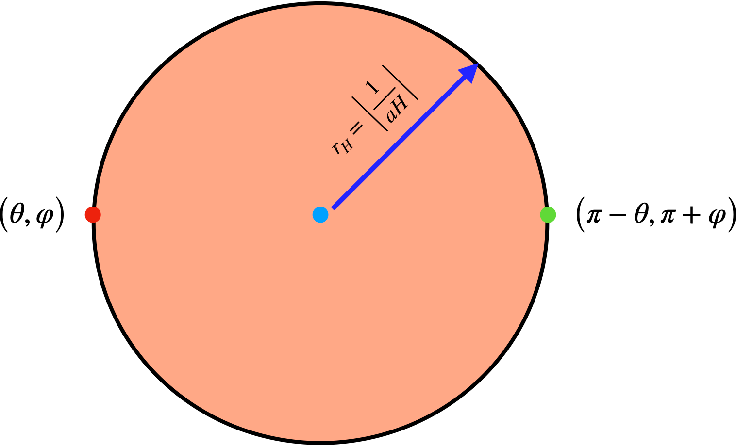
Figure 10: Depiction of the co-moving horizon in the de Sitter Universe in flat FLRW coordinates where the points $\left(\theta,\,\varphi\right)$ and $\left(\pi-\theta,\,\pi+\varphi\right)$ are always causally separated.

The description of a quantum field in such a curved spacetime is very non-trivial especially when the quantum field is described by a vacuum that contains an infinite pair of parity conjugate points on the horizon that are space-like separated. In other words, it is inconceivable to decipher a single propagator that connects the points $\left(\theta,\,\varphi\right)$ and $\left(\pi-\theta,\,\pi+\varphi\right)$ on the particle horizon, otherwise we would violate causality. In the standard QFT in Minkowski spacetime, the Feynman propagator vanishes exponentially outside the light cone. So conceptually it is convincing to think propagator of a quantum field in any given spacetime must not involve space-like distances. Within this principle, we run into trouble describing the quantum field in an inflationary Universe because, by construction, the pairs of parity opposite points on the horizon are always space-like separated at every moment of the expansion.

Let us turn now our attention to the metric (45) which has a symmetry

$$\Big{\{}t\to-t,\,H\to-H\Big{\}}\implies\Big{\{}\tau\to-\tau\Big{\}},\quad\Big{\{}\textbf{x}\to-\textbf{x}\Big{\}}$$ (48)

Time reversal and space reflection are the usual ${\mathcal{P}}{\mathcal{T}}$ operations that we know in quantum field theory. Here we see a new (quantum) parameter $H$ that has a reflection symmetry in de Sitter space which does not affect the value of scalar curvature $R=12H^{2}$. This can be understood in another way by rewriting the metric (45) in conformal time $\tau$

$$ds^{2}=\frac{1}{\tau^{2}H^{2}}\left(-d\tau^{2}+d\textbf{x}^{2}\right)$$ (49)

which is clearly a metric that is conformal to Minkowski spacetime with the same discrete symmetry (48) which is time ($\tau$) reversal and space-reflection. What this conveys is that the nature of the expanding Universe is associated with the growth of scale factor (or shrinking co-moving particle horizon) is consistent with both signs $\tau<0$ and $\tau>0$. Often in the literature, $\tau<0$ is fixed before quantization of a field in de Sitter space. This leads to conundrums since another choice of time $\tau>0$ is equally possible. A physical conundrum here is how can quantum fields in the time-symmetric ($\tau\to-\tau$) spacetime (49) distinguish $\tau<0$ with $\tau>0$? It is important to note here that the singularity $\tau\to 0$ in the metric (49) is a coordinate singularity as the de Sitter metric (45) is a completely regular one. Therefore, $\tau\to 0$ singularity cannot be a reason to make a conscious choice $\tau>0$ or $\tau<0$.

7.3.2 Observer complimentarity principle

A regular practice in theoretical cosmology is to assume $\tau<0$ or $\tau>0$ which are often called Poincaré patches of de Sitter space and they have always been read as either two (entangled) Universes that are causally disconnected or only one universe is the real physical world while other being regarded as unphysical by hand Spradlin:2001pw ; Hartman:2020khs . It is remarkable that Schrödinger in 1956 rejected the idea of two Universes and demanded there should be only one Universe Schrodinger1956 ; Parikh:2002py . This is based on a basic principle that physics of any observer should not depend on the physics happening outside his/her horizon. This is called the observer complementarity principle which has been realized in the form of DQFT with recent developments Kumar:2022zff ; Kumar:2023ctp ; Kumar:2023hbj .

7.4 DQFT for inflationary quantum fluctuations

It is good to recall again that the inflationary paradigm by definition is a regime of quasi-de Sitter phase in the early Universe Starobinsky:1980te ; Guth:1980zm . The de Sitter metric (45) has a discrete symmetry (${\mathcal{P}}{\mathcal{T}}$) (48) that inflationary spacetime breaks by the background dynamics of the scalar field that rolls down the potential. The slow-roll parameters (29) break the symmetry (48) classically. A legitimate question here is what is the response of the quantum fluctuations to this symmetry breaking and what is the imprint of it in the CMB? The standard formulation of inflationary quantum fluctuations is insensitive to this fundamental fact about classical inflationary background breaking the discrete symmetry of de Sitter spacetime. It is worth pointing out here that discrete spacetime transformations take a central spot in our understanding of quantum theory and we refer the reader to Kumar:2023ctp for detailed discussions on this topic.

7.4.1 Direct-sum QM and QFT

Direct-sum quantum mechanics (QM) is rewriting standard QM in a more symmetric form. Here Direct-sum means

We define a quantum state as a direct-sum of two components, which are the states in parity conjugate regions of space corresponding to two Hilbert spaces whose direct-sum forms the total Hilbert space. Thus, a single quantum state in direct-sum QM evolves forward and backward in time in the parity conjugate regions of physical space.

The above text can be translated to the equations as

$$|\Psi\rangle=\frac{1}{\sqrt{2}}\left(|\Psi_{+}\rangle\oplus|\Psi_{-}\rangle\right)=\frac{1}{\sqrt{2}}\begin{pmatrix}|\Psi_{+}\rangle\\ |\Psi_{-}\rangle\end{pmatrix}$$ (50)

which obeys the direct-sum Schrödinger equation

$$i\frac{\partial|\Psi\rangle}{\partial t_{p}}=\begin{pmatrix}\hat{\mathbb{H}}&0\\ 0&-\hat{\mathbb{H}}\end{pmatrix}|\Psi\rangle$$ (51)

where $\mathbb{H}$ is the time-independent Hamiltonian (which is Hermitian) that is ${\mathcal{P}}{\mathcal{T}}$ symmetric. One can immediately notice from the above equation that the components evolve as

$$|\Psi_{+}\rangle_{t_{p}}=e^{-i\mathbb{H}t_{p}}|\Psi_{+}\rangle_{0},\quad|\Psi_{-}\rangle_{t_{p}}=e^{+i\mathbb{H}t_{p}}|\Psi_{-}\rangle_{0}$$ (52)

which are positive energy components evolving forward and backward in time. To be more precise the component $|\Psi\rangle_{+}$ is defined only in a spatial region $x\gtrsim 0$ whose time evolution is governed by

$$i\frac{\partial}{\partial t_{p}}|\Psi_{+}\rangle=\mathbb{H}|\Psi_{+}\rangle$$ (53)

which is a positive energy state with a parametric convention on the arrow of time $t_{p}:-\infty\to\infty$ whereas the component $|\Psi\rangle_{-}$ is defined only in a spatial position $x\lesssim 0$ whose time evolution is governed by

$$-i\frac{\partial}{\partial t_{p}}|\Psi_{-}\rangle=\mathbb{H}|\Psi_{-}\rangle$$ (54)

which is a positive energy state with a parametric convention for the arrow of time $t_{p}:\infty\to-\infty$. Both $\Psi_{+}$ and $\Psi_{-}$ are the states corresponding to two direct-sum Hilbert spaces associated with the parity conjugate spatial regions $x>0$ and $x<0$ respectively.

$$\mathtt{H}=\mathtt{H}_{+}\oplus\mathtt{H}_{-}\implies\Big{[}\hat{{\mathcal{O}}}_{+},\,\hat{{\mathcal{O}}}_{-}\Big{]}=0\,.$$ (55)

where ${\mathcal{O}}_{+},\,{\mathcal{O}}_{-}$ are the operators that act on the states of Hilbert spaces $\mathtt{H}_{+},\,\mathtt{H}_{-}$ respectively.

From (50) we can deduce that

$$\langle\Psi|\Psi\rangle=\frac{1}{2}\langle\Psi_{+}|\Psi_{+}\rangle+\frac{1}{2}\langle\Psi_{-}|\Psi_{-}\rangle=1,$$ (56)

Since $\langle\Psi_{+}|\Psi_{+}\rangle=\langle\Psi_{-}|\Psi_{-}\rangle=1$ are the probability densities in each Hilbert space are unity. The wavefunction is obtained by

$$\begin{aligned} \Psi\left(x,\,t_{p}\right)&=\langle x|\Psi\rangle_{t_{p}}=\frac{1}{2}\begin{pmatrix}\langle x_{+}|&\langle x_{-}|\end{pmatrix}\begin{pmatrix}|\Psi_{+}\rangle_{t_{p}}\\ |\Psi_{-}\rangle_{t_{p}}\end{pmatrix}=\frac{1}{2}\langle x_{+}|\Psi_{+}\rangle_{t_{p}}+\frac{1}{2}\langle x_{-}|\Psi_{-}\rangle_{t_{p}}\\ &=\frac{1}{2}\Psi_{+}\left(x_{+}\right)+\frac{1}{2}\Psi_{-}\left(x_{-}\right)\end{aligned}\,,$$ (57)

which conveys the information that the total wave function of the physical system is the sum of the wave functions of the parity conjugate regions defined by the position vectors $|x_{+}\rangle$ and $|x_{-}\rangle$ respectively. We can clearly witness here that the wave-function of direct-sum QM is ${\mathcal{P}}{\mathcal{T}}$ symmetric for a ${\mathcal{P}}{\mathcal{T}}$ symmetric physical system described by $\mathbb{H}$. We can easily apply the direct-sum QM for the harmonic oscillator case which does not change any results in practice but rather it brings a new understanding of having the ${\mathcal{P}}{\mathcal{T}}$ symmetry in the physical system. The quantum harmonic oscillator in direct-sum QM is described by

$$\hat{x}_{+} =\sqrt{\frac{1}{2}}\left(a+a^{\dagger}\right),\quad\hat{p}_{+}=-i\frac{d}{dx_{+}}=\frac{i}{\sqrt{2}}\left(a^{\dagger}-a\right)$$ (58)

$$\hat{x}_{-} =\sqrt{\frac{1}{2}}\left(b+b^{\dagger}\right),\quad\hat{p}_{-}=i\frac{d}{dx_{-}}=-\frac{i}{\sqrt{2}}\left(b^{\dagger}-b\right)$$

with

$$\Big{[}\hat{x}_{+},\,\hat{p}_{+}\Big{]} =i,\quad\Big{[}\hat{x}_{-},\,\hat{p}_{-}\Big{]}=-i$$ (59)

$$\Big{[}a,\,a^{\dagger}\Big{]} =\Big{[}b,\,b^{\dagger}\Big{]}=1,\quad\Big{[}a,\,b^{\dagger}\Big{]}=\Big{[}a,\,b\Big{]}=0\,.$$

The wavefunction of the Harmonic oscillator is

$$\Psi\left(x,\,t_{p}\right) =\frac{1}{\sqrt{2}}\Psi_{+}\left(t_{p},\,x_{+}\right)+\frac{1}{\sqrt{2}}\Psi_{-}\left(-t_{p},\,x_{-}\right)$$ (60)

$$=\frac{1}{\sqrt{2^{n+1}n!}}\left(\frac{1}{\pi}\right)^{1/4}e^{-x_{+}^{2}}H_{n}\left(x_{+}\right)e^{-iE_{n}t_{p}}+\frac{1}{\sqrt{2^{n+1}n!}}\left(\frac{1}{\pi}\right)^{1/4}e^{-x_{-}^{2}}H_{n}\left(x_{-}\right)e^{iE_{n}t_{p}}$$

where $H_{n}(z)$ is the Hermite Polynomial. and the probability density is

$$\Big{|}\Psi\left(x,\,t_{p}\right)\Big{|}^{2} ={}_{t_{p}}\langle\Psi|\Psi\rangle_{t_{p}}=\frac{1}{2}\Big{|}\Psi_{+}\left(x_{+},\,t_{p}\right)\Big{|}^{2}+\frac{1}{2}\Big{|}\Psi_{-}\left(x_{-},\,t_{p}\right)\Big{|}^{2}$$ (61)

Now we turn our attention to the DQFT in Minkowski spacetime

$$ds^{2}=-dt_{m}^{2}+d\textbf{x}^{2}\,.$$ (62)

According to DQFT, the Klein-Gordon field in Minkowski spacetime is quantized as

$$\hat{\phi}\left(x\right) =\frac{1}{\sqrt{2}}\hat{\phi}_{+}\left(t_{m},\,\textbf{x}\right)\oplus\frac{1}{\sqrt{2}}\hat{\phi}_{-}\left(-t_{m},\,-\textbf{x}\right)$$ (63)

$$=\frac{1}{\sqrt{2}}\begin{pmatrix}\hat{\phi}_{+}&0\\ 0&\hat{\phi}_{-}\end{pmatrix}$$

where

$$\hat{\phi}_{+}\left(x\right) =\int\frac{d^{3}k}{\left(2\pi\right)^{3/2}}\frac{1}{\sqrt{2|k_{0}|}}\Bigg{[}\hat{a}_{(+)\,\textbf{k}}e^{ik\cdot x}+\hat{a}^{\dagger}_{(+)\,\textbf{k}}e^{-ik\cdot x}\Bigg{]}$$ (64)

$$\hat{\phi}_{-}\left(-x\right) =\int\frac{d^{3}k}{\left(2\pi\right)^{3/2}}\frac{1}{\sqrt{2|k_{0}|}}\Bigg{[}\hat{a}_{(-)\,\textbf{k}}e^{-ik\cdot x}+\hat{a}^{\dagger}_{(-)\,\textbf{k}}e^{ik\cdot x}\Bigg{]}$$

The creation and annihilation operators satisfy

$$=[\hat{a}_{(-)\,\textbf{k}},\,\hat{a}_{(-)\,\textbf{k}^{\prime}}^{\dagger}]=\delta^{(3)}\left(\textbf{k}-\textbf{k}^{\prime}\right)$$ (65)

$$[\hat{a}_{(+)\,\textbf{k}},\,\hat{a}_{(-)\,\textbf{k}^{\prime}}] =[\hat{a}_{(+)\,\textbf{k}},\,\hat{a}_{(-)\,\textbf{k}^{\prime}}^{\dagger}]=0\,.$$

Furthermore, the commutation relations of the field and the corresponding conjugate momenta become

$$[\hat{\phi}_{(+)}\left(t_{m},\textbf{x}\right),\,\pi_{(+)}\left(t_{m},\,\textbf{x}^{\prime}\right)]=i\delta\left(\textbf{x}-\textbf{x}^{\prime}\right),\quad[\hat{\phi}_{(-)}\left(-t_{m},-\textbf{x}\right),\,\pi_{(-)}\left(-t_{m},\,-\textbf{x}^{\prime}\right)]=-i\delta\left(\textbf{x}-\textbf{x}^{\prime}\right),$$ (66)

where

$$\pi_{(+)}\left(t_{m},\,\textbf{x}\right)=\frac{\partial{\mathcal{L}}_{\rm KG}}{\partial\left(\partial_{t_{m}}\phi_{(+)}\right)},\quad\pi_{(-)}\left(t_{m},\,\textbf{x}\right)=-\frac{\partial{\mathcal{L}}_{\rm KG}}{\partial\left(\partial_{t_{m}}\phi_{(-)}\right)}$$ (67)

where ${\mathcal{L}}$ is the Lagrangian of the Klein-Gordan field. We now define Fock space vacuums as

$$\hat{a}_{+\,\textbf{k}}|0_{+}\rangle=0,\quad\hat{a}_{-\,\textbf{k}}|0_{-}\rangle=0\,,$$ (68)

The total Fock space vacuum state is given by

$$|0_{T}\rangle=|0_{+}\rangle\oplus|0_{-}\rangle=\begin{pmatrix}|0_{+}\rangle\\ |0_{-}\rangle\ \end{pmatrix}\,.$$ (69)

In the DQFT the scalar field propagator which is by definition a time-ordered product of a two-point function is split into two parts as

$$\langle 0_{T}|{\mathcal{T}}\hat{\phi}\left(x\right)\hat{\phi}\left(y\right)|0_{T}\rangle=\langle 0_{+}|{\mathcal{T}}\hat{\phi}_{+}\left(x\right)\hat{\phi}_{+}\left(y\right)|0_{+}\rangle+\langle 0_{-}|{\mathcal{T}}\hat{\phi}_{-}\left(x\right)\hat{\phi}_{-}\left(y\right)|0_{-}\rangle$$ (70)

According to DQFT in Minkowski spacetime, $\hat{\phi}|0\rangle_{T}=\begin{pmatrix}\hat{\phi}_{+}|0_{+}\rangle\\ \hat{\phi}_{-}|0_{-}\rangle\ \end{pmatrix}$ leads to a quantum state that evolve forward in time at x and backward in time at $-\textbf{x}$. Further details of DQFT in Minkowski spacetime can be found in Kumar:2023ctp .

7.5 DQFT inflationary fluctuations

When we do quantization of inflationary fluctuations we promote the canonical variable (27) as an operator $\hat{v}$ which according to the rules of DQFT transformed as

$$\hat{v} =\frac{1}{\sqrt{2}}\hat{v}_{(+)}\left(\tau,\,\textbf{x}\right)\oplus\frac{1}{\sqrt{2}}\hat{v}_{(-)}\left(-\tau,\,-\textbf{x}\right)$$ (71)

$$=\frac{1}{\sqrt{2}}\begin{pmatrix}\hat{v}_{(+)}\left(\tau,\,\textbf{x}\right)&0\\ 0&\hat{v}_{-}\left(-\tau,\,-\textbf{x}\right)\end{pmatrix}$$

where

$$\hat{v}_{\pm}\left(\pm\tau,\,\pm\textbf{x}\right)=\int\frac{d^{3}k}{\left(2\pi\right)^{3/2}}\Bigg{[}c_{\left(\pm\right)\textbf{k}}{v}_{\pm,\,k}e^{\pm i\textbf{k}\cdot\textbf{x}}+c_{\left(\pm\right)\textbf{k}}^{\dagger}{v}_{\pm,\,k}^{\ast}e^{\mp i\textbf{k}\cdot\textbf{x}}\Bigg{]}$$ (72)

with $c_{\left(\pm\right)\textbf{k}},\,c_{\left(\pm\right)\textbf{k}}^{\dagger}$ being the creation and annihilation operators of quasi de Sitter (qdS) vacua defined by

$$c_{\left(+\right)\textbf{k}}|0\rangle_{\rm qdS_{I}} =0\quad c_{\left(-\right)\textbf{k}}|0\rangle_{\rm qdS_{II}}=0$$ (73)

$$\big{[}c_{\left(\pm\right)\textbf{k}},\,c_{\left(\pm\right)\textbf{k}^{\prime}}^{\dagger}\big{]} =\delta\left(\textbf{k}-\textbf{k}^{\prime}\right),\quad\big{[}c^{\dagger}_{\left(\pm\right)\textbf{k}},\,c^{\dagger}_{\left(\mp\right)\textbf{k}^{\prime}}\big{]}=0$$

The total inflationary vacuum is a direct-sum

$$|0\rangle_{\rm qdS}=|0\rangle_{\rm qdS_{I}}\oplus|0\rangle_{\rm qdS_{II}}=\begin{pmatrix}|0\rangle_{\rm qdS_{I}}\\ |0\rangle_{\rm qdS_{II}}\end{pmatrix}$$ (74)

and ${v}_{\pm,\,k}$ are the mode functions obtained by solving Mukhanov-Sasaki (MS) equation for $v_{\pm}$

$$v_{\pm,\,k}^{\prime\prime}+\left(k^{2}-\frac{{\nu}_{s}^{\left(\pm\right)2}-\frac{1}{4}}{\tau^{2}}\right)v_{\pm,\,k}^{2}=0\,.$$ (75)

where

$$\nu_{s}^{\pm}\approx\frac{3}{2}\pm\epsilon\pm\frac{\eta}{2}$$ (76)

Here where $v_{(+)}|0\rangle_{\rm qdS_{I}}$ gives a field component evolving forward in time ($\tau:-\infty\to 0$) whereas $v_{(-)}|0\rangle_{\rm qdS_{II}}$ ($\tau:\infty\to 0$) in the parity conjugate regions x and $-\textbf{x}$ respectively. Note that time reversal operation (in a completely quantum mechanical sense) is given by

$$t\to-t\implies\tau\to-\tau\implies H\to-H,\,\epsilon\to-\epsilon\,,\eta\to-\eta\,.$$ (77)

which conveys that in the context of gravity time reversal operation is much more than what we know in the context of quantum mechanics. Here the slow-roll parameters $\epsilon,\,\eta$ classically break the time-reversal symmetry of de Sitter space (48). Therefore, the quantum field in the inflationary space-time breaks the ${\mathcal{P}}{\mathcal{T}}$ symmetry of de Sitter space due to (77) in our framework of DQFT.

The solutions for the mode functions are

$${v}_{\pm,\,k}=\frac{\sqrt{\mp\pi\tau}}{2}e^{\left(i\nu_{s}^{\pm}+1\right)}\Bigg{[}C_{k}^{\pm}H^{(1)}_{\nu_{s}^{\pm}}\left(\mp k\tau\right)+D_{k}^{\pm}H^{(2)}_{\nu_{s}^{\pm}}\left(\mp k\tau\right)\Bigg{]}.$$ (78)

The canonical commutation relations

$$\Big{[}\hat{v}_{\pm},\,\hat{v}_{\pm}^{\prime}\Big{]}=\pm i$$ (79)

gives us

$$|C_{k}^{\pm}|^{2}-|D_{k}^{\pm}|^{2}=1\,.$$ (80)

We choose the adiabatic vacuum that corresponds to

$$\left(C_{k}^{\pm},\,D_{k}^{\pm}\right)=\left(1,\,0\right)\,.$$ (81)

The two-point function of the canonical variable is

$${}_{\rm qdS}\langle 0|\hat{v}\left(\tau,\,\textbf{x}\right)\hat{v}\left(\tau,\,\textbf{y}\right)|0\rangle_{\rm qdS}= \,\frac{1}{2}{}_{\rm qdS_{I}}\langle 0|\hat{v}_{+}\left(\tau,\,\textbf{x}\right)\hat{v}_{(+)}\left(\tau,\,\textbf{y}\right)|0\rangle_{\rm qdS_{I}}$$ (82)

$$+\frac{1}{2}{}_{\rm qdS_{II}}\langle 0|\hat{v}_{-}\left(-\tau,\,-\textbf{x}\right)\hat{v}_{-}\left(-\tau,\,-\textbf{y}\right)|0\rangle_{\rm qdS_{II}}$$

$$= \,\frac{1}{2}\int\frac{dk}{k}\frac{k^{3}}{2\pi^{2}}\left(|v_{+\,k}|^{2}+|v_{-\,k}|^{2}\right)\frac{\sin{kL}}{kL}$$

where $L=|\textbf{x}-\textbf{y}|$. The power spectrum related to the canonical variable is given by

$${}_{\rm qdS}\langle 0|\hat{v}_{\textbf{k}}\hat{v}_{\textbf{k}^{\prime}}|0\rangle_{\rm qdS} =\frac{1}{2}{}_{\rm qdS_{I}}\langle 0|\hat{v}_{(+),\,\textbf{k}}\hat{v}_{(+),\,\textbf{k}^{\prime}}|0\rangle_{\rm qdS_{I}}+\frac{1}{2}{}_{\rm qdS_{II}}\langle 0|\hat{v}_{(-),\,\textbf{k}}\hat{v}_{(-),\,\textbf{k}^{\prime}}|0\rangle_{\rm qdS_{II}}$$ (83)

$$=\delta\left(\textbf{k}+\textbf{k}^{\prime}\right)\frac{2\pi^{2}}{k^{3}}{\mathcal{P}}_{v}$$

where

$$\hat{v}_{(\pm)\,\textbf{k}}=\int\frac{d^{3}x}{\left(2\pi\right)^{3/2}}\hat{v}_{(\pm)}\left(\pm\tau,\,\pm\textbf{x}\right)e^{-i\textbf{k}\cdot\textbf{x}}$$ (84)

and

$${\mathcal{P}}_{v} =\frac{1}{2}|v_{(+)\,k}|^{2}+\frac{1}{2}|v_{(-)\,k}|^{2}$$ (85)

where

$${\mathcal{P}}_{v}^{\pm}=|v_{(\pm)\,k}|^{2}\approx\frac{1}{2}\frac{\pi|\tau|}{2}\Bigg{|}H_{3/2}^{(1)}\left(\mp k\tau\right)\Bigg{|}^{2}\left(1\pm\Delta{\mathcal{P}}_{v}\right)$$ (86)

which conveys the power spectrum of quantum fluctuation $v$ has a parity antisymmetric component

$$\Delta{\mathcal{P}}_{v}=\left(2\epsilon+\eta\right)\operatorname{Re}\left[\frac{1}{H_{3/2}^{(1)}\left(\mp k\tau\right)}\frac{\partial H^{(1)}_{\nu_{s}}\left(\mp k\tau\right)}{\partial\nu_{s}}\Bigg{|}_{\nu_{s}=\frac{3}{2}}\right]$$ (87)

The power spectrum of the curvature perturbation can be obtained by (classical) rescaling from (27) which we evaluate at a moment of a mode $k_{\ast}=a_{\ast}H_{\ast}$ which exits the horizon approximately 55-60 e-folds before the end of inflation

$${\mathcal{P}}_{\zeta} =\frac{1}{2a^{2}\epsilon}\Bigg{|}_{\rm classical}{\mathcal{P}}_{v}\Bigg{|}_{\tau=\mp\frac{1}{a_{\ast}H_{\ast}}}$$ (88)

$$\approx\frac{H_{\ast}^{2}}{8\pi\epsilon_{\ast}}\left(\frac{k}{k_{\ast}}\right)^{n_{s}-1}\frac{1}{2}\left[\left(1+\Delta{\mathcal{P}}_{v}\left(\frac{k}{k_{\ast}}\right)\right)+\left(1-\Delta{\mathcal{P}}_{v}\left(\frac{k}{k_{\ast}}\right)\right)\right]$$

$$\approx A_{s}\left(\frac{k}{k_{\ast}}\right)^{n_{s}-1}$$

where $A_{s}=2.2\times 10^{-9}$ from the Planck data with $k_{\ast}=0.05{\rm Mpc}^{-1}$. In our DSI approach developed above, the antisymmetric component of the primordial fluctuations $\Delta{\mathcal{P}}_{v}$ will result in an antisymmetric $\Delta T$ CMB component under parity transformation: $\Delta{\mathcal{T}}\left(\hat{n}\right)=-\Delta{\mathcal{T}}\left(-\hat{n}\right)$ which translates into $\Delta a_{\ell m}$ of $\Delta{\mathcal{P}}_{v}$ equal to zero for even modes, as shown in (13). With our method of calculation, the scale-dependent correction $\Delta{\mathcal{P}}_{v}\left(\frac{k}{k_{\ast}}\right)$ is accurate enough for the modes $k<k_{c}$ that must have already exited the horizon much before $k_{\ast}$ which corresponds to $55-$efoldings in our consideration. From the latest Planck data Planck:2018jri the value of spectral index $n_{s}$ corresponding to the pivot scale $k_{\ast}$ is

$$n_{s}=1-2\epsilon_{\ast}-\eta_{\ast}\approx 0.9634\pm 0.0048\quad\left(\rm{PlanckTT+TE+EE}\right)$$ (89)

which we use it to estimate $\Delta{\mathcal{P}}_{v}$ as shown in Fig. 11.

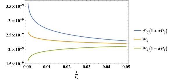
Figure 11: In this plot, we depict the power spectrum of curvature perturbation ${\mathcal{P}}_{\zeta}$ (88) with its antisymmetric components. The corresponding values are displayed in Table 4.

$k<k_{c}$	DSI25	DSI	DSI50	15.8 percentile	84.1 percentile
$\ell$	$k_{c}=ks/25$	$k_{c}=ks/40$	$k_{c}=ks/50$	$10^{6}$ SMICm realizations
1	1.475	1.471	1.468
2	0.582	0.589	0.594	0.473	1.824
3	1.385	1.373	1.363	0.549	1.637
4	0.641	0.657	0.667	0.593	1.545
5	1.339	1.320	1.305	0.634	1.470
6	0.678	0.705	0.725	0.649	1.455
7	1.305	1.278	1.258	0.674	1.412
8	0.708	0.743	0.770	0.687	1.395
9	1.277	1.235	1.199	0.705	1.365
10	0.734	0.776	0.814	0.714	1.355
11	1.254	1.203	1.168	0.727	1.331
12	0.759	0.824	0.875	0.734	1.324
13	1.233	1.165	1.073	0.745	1.309
14	0.781	0.845	0.967	0.750	1.301
15	1.208	1.126	1.012	0.759	1.288
16	0.799	0.916	0.996	0.759	1.288
17	1.188	1.045	1.001	0.759	1.288
18	0.825	0.980	1.000	0.759	1.288
19	1.169	1.007	1.000	0.780	1.259
20	0.840	0.998	1.000	0.783	1.256
21	1.143	1.001	1.000	0.783	1.256
22	0.871	1.000	1.000	0.792	1.244
23	1.124	1.000	1.000	0.797	1.237
24	0.882	1.000	1.000	0.799	1.234
25	1.102	1.000	1.000	0.799	1.234
26	0.925	1.000	1.000	0.799	1.234
27	1.047	1.000	1.000	0.799	1.234
28	0.974	1.000	1.000	0.811	1.219
29	1.012	1.000	1.000	0.814	1.214
30	0.995	1.000	1.000	0.828	1.229
31	1.002	1.000	1.000	0.841	1.239
32	0.999	1.000	1.000	0.779	1.144
33	1.000	1.000	1.000	0.809	1.180

Table 4: Values for $1\pm\Delta{\mathcal{C}}_{\ell}$ in (103) for the DSI model with different approximations for the cut-off $k_{c}$. The last two columns give the percentiles 15.8 and 84.1 (corresponding to $\pm 1\sigma$ range for a Gaussian distribution) in the relative $C_{\ell}$ measurements over $10^{6}$ sampling variance realizations of the SMIC_m Planck CMB maps. The corresponding simulated outputs are displayed in Fig. 16 and Fig. 5. The significance of odd parity in the first individual multipoles is only about $1\sigma$, but each multipole is approximately independent, which means that such odd parity can potentially be measured with a large significance within $\ell<30$.

Using (15) we obtain the temperature angular power spectrum for the even and odd multipoles as

$$C_{\ell}^{odd}=\frac{2}{9\pi}\int_{0}^{k_{c}}\frac{dk}{k}j_{\ell}^{2}\left(\frac{k}{k_{s}}\right)\frac{H^{2}}{8\pi\epsilon}\left(1+\Delta{\mathcal{P}}_{v}\right)$$ (90)

$$C_{\ell}^{even}=\frac{2}{9\pi}\int_{0}^{k_{c}}\frac{dk}{k}j_{\ell}^{2}\left(\frac{k}{k_{s}}\right)\frac{H^{2}}{8\pi\epsilon}\left(1-\Delta{\mathcal{P}}_{v}\right)$$

In summary, according to DQFT, quantum fluctuations evolve forward and backward in time in the two parity conjugate regions. Although the total power spectrum of the fluctuation matches with the standard (near) scale-invariant power spectrum, the antisymmetric component (87) leads to an asymmetry in power in the parity conjugate regions. This is pictorially depicted in Fig. 3.

7.6 The power spectrum of DSI and the first modes to exit horizon

At first glance, the power spectrum of DSI (88) may appear to be very simple but the physics of it is rather profound. Recalling once again the concept that in DSI a quantum fluctuation is generated as a direct-sum of two opposite time-evolving components at the parity pair of points in physical space. The total power spectrum (88) is the average of power at the parity conjugate pair of points in the homogeneous and isotropic spacetime. In other words, in DSI the primordial power is distributed unequally into the parity conjugate points in physical space, and when we take the average we recover exactly the power-law form of the power spectrum which has been the best-fit description of the CMB excluding the low-$\ell$ anomalies.

The antisymmetric component of the power spectrum (87) is evaluated for the modes of interest $k\lesssim 0.001\,\rm{Mpc}^{-1}$ which are the ones to exit the horizon much before the mode $k=0.05\,\rm{Mpc}^{-1}$. The reason we impose $k\lesssim 0.001\,\rm{Mpc}^{-1}$ for the antisymmetric component of the power spectrum is that the modes do not immediately become frozen after the horizon exit. From now on we refer to the results of SI in the literature whose conclusions are generically valid for DSI as well. The time evolution of curvature perturbation is determined by the following equation

$$\zeta_{k}^{\prime\prime}+2\frac{z^{\prime}}{z}\zeta_{k}+k^{2}\zeta_{k}=0\,.$$ (91)

where $z=a\frac{\dot{\phi}}{H}$ which is the classical rescaling factor that relates the canonical variable and curvature perturbation (27). At the horizon exit i.e., when $k\sim aH$ the decaying component of the curvature perturbation given below takes a few e-folds (about 3 to 4) after which the constant component dominates Polarski:1995jg ; Julien

$$\zeta_{k}=G_{k}+F_{k}\int\frac{dt}{a^{3}\epsilon}$$ (92)

where $G_{k},\,F_{k}$ are the $k$-dependent constants. The solution for $\zeta_{k}$ (92) can be obtained from solving (91) in the limit $k\to 0$. Following the numerical evaluations of (34) and the corresponding curvature perturbation in SI, one can reach sufficient accuracy in evaluating the primordial power spectrum by evolving each mode at least a factor of 50 times before the mode exits the horizon Julien . Alternatively, we determine the power spectrum of $k$ at a moment of $aH$ at least 50 times larger. This is exactly the upper cut-off we used in our calculation of the angular power spectrum and the antisymmetric component in DSI. Moreover, the scales $10^{-4}\,\rm{Mpc}^{-1}<k\lesssim 0.001\,\rm{Mpc}^{-1}$ corresponds to approximately $\ell=2-30$ where CMB anomalies are centered in. These are the scales $k<0.02k_{\ast}$ where the pivot scale $k_{\ast}$ corresponds to $\ell=200$. Therefore, for the investigation carried out in this paper, we sufficiently computed the primordial power spectrum of DSI to the particular modes of interest (that have exited the horizon much before the onset of inflation corresponding to the pivot scale $k_{\ast}$) to confront against the latest CMB data. From the point of view of DSI, the parity asymmetry of the power spectrum for the high-energy modes is expected to become small because the effects of curved spacetime on quantum fields should cease to exist as we go to high-energy modes. This is exactly what we can observe in Fig. 11 which is accurate up to an order of magnitude smaller than the pivot scale as the remaining modes would be in the process of quantum-to-classical transition impacted by the modes that have already left the horizon.

The quantum-to-classical transition of inflationary fluctuations is the whole subject of separate investigation Kiefer:1998qe ; Sudarsky:2009za ; Landau:2011ljv . Inflationary fluctuations once they become classical would leave their imprint as in-homogeneities and anisotropies which we can probe now using CMB and primordial gravitational waves. The first scalar modes that leave the horizon at the beginning of inflation would leave large-scale in-homogeneities which affect the modes that leave at a later stage. This is because inflationary quantum fluctuations leaving the horizon and evolving into classical ones is a non-Markovian process Cruces:2022imf . To accurately capture the correlations of all modes, it is more appropriate to employ the scheme of Stochastic inflation Starobinsky:1983zz where the scalar field fluctuations are split into the long and short wavelength modes as

$$\phi\left(N,\,\textbf{x}\right)=\phi_{cg}\left(N,\,\textbf{x}\right)+\delta\hat{\phi}\left(N,\,\textbf{x}\right)$$ (93)

where $\phi_{cg}\left(\tau,\,\textbf{x}\right)$ is the coarse-grained field (non-expanding) at a fixed scale that contains the classical modes that have already left the horizon long before the later modes. This contribution already leaves in-homogeneities within the Hubble patch which determine the short-wavelength modes which are called the Stochastic noise or white noise described as

$$\delta\hat{\phi}=\frac{1}{\left(2\pi\right)^{3/2}}\int d^{3}k\,\Theta(k-\sigma aH)\left[\hat{s}\phi_{k}\left(\tau\right)e^{-i\textbf{k}\cdot\textbf{x}}+\hat{s}^{\dagger}\phi_{k}^{\ast}\left(\tau\right)e^{i\textbf{k}\cdot\textbf{x}}\right]\,,$$ (94)

where $\sigma\ll 1$ determine coarse-graining modes. The annihilation and creation operators characterize the modes that are shorter in wavelength than the coarse-graining modes. The splitting of the field into classical and quantum/stochastic parts (93) in Stochastic formalism gives the effective quantum dynamics of long-wavelength modes. In (94) is the most popular way to introduce a cut-off between infrared (IR) long wavelength and UV short wavelength modes, but instead of a sharp cut-off more realistic smooth functions have been studied recently Mahbub:2022osb . As inflation proceeds contribution to the coarse-grained field increases due to the continuous quantum kicks from the short-wavelength modes that later evolve to be classical. This is called the quantum backreaction which has been explored in the context of primordial black holes during inflation Pattison:2017mbe ; Pattison:2019hef . The stochastic framework is to study inflationary fluctuations in a non-perturbative manner and the technique in several instances has been proven to be powerful and match the predictions of standard QFT methods Finelli:2001bn ; Tsamis:2005hd ; Finelli:2011gd ; Finelli:2008zg . The free parameter $\sigma\ll 1$ is used for gradient expansion of the perturbed metric of the long wavelength modes in the Stochastic framework.

Having the long wavelength modes becoming classical, the Universe will only be locally homogeneous and isotropic with the following local scale factor and the Hubble parameter which are estimated to the first order in gradient expansion ($\sigma$) of the perturbed quantities Cruces:2022imf

$$a_{\ell}\approx a(t)e^{-\int\partial_{i}{\mathcal{N}}_{cg}^{i}dt},\quad H_{\ell}\approx\frac{H}{{\mathcal{N}}_{cg}}-\frac{1}{3{\mathcal{N}}_{cg}}\partial_{i}{\mathcal{N}}_{cg}^{i}\,.$$ (95)

Once we split the perturbed quantities into the IR and UV parts by the characteristic scale $k_{\sigma}=\sigma aH$

$$\zeta_{k}=\zeta_{k<k_{\sigma}}+\zeta_{k>k_{\sigma}}\,,$$ (96)

the Lapse and Shift functions ${\mathcal{N}},\,{\mathcal{N}}_{i}$ are also split into IR and UV parts. In the spatially flat gauge, the curvature perturbation is proportional to the inflaton field fluctuation as

$$\zeta=-\frac{H}{\dot{\phi}}\delta\phi\,,$$ (97)

and the Lapse and Shift are given by

$${\mathcal{N}}\approx 1+\sqrt{\frac{\epsilon}{2}}\delta\phi,\quad\partial_{i}{\mathcal{N}}^{i}\approx-aH^{2}\left(\frac{\partial\delta\phi}{\partial N}-\frac{\eta}{2}\delta\phi\right)$$ (98)

The non-Markovian nature of inflationary quantum fluctuations can be seen by the Stochastic differential equations (in the units of $M_{p}=1$) given by

$$\pi_{cg}=\frac{\partial\phi_{cg}}{\partial N}+\xi_{1}$$ (99)

$$\frac{\partial\pi_{cg}}{\partial N}+\left(3-\frac{\pi_{cg}^{2}}{2}\right)\left(\pi_{cg}+\frac{V_{,\,\phi_{cg}}\left(\phi_{cg}\right)}{V}\right)=-\xi_{2}\,.$$

where

$$\xi_{1} =-\frac{\partial}{\partial N}\left(\frac{\sigma aH}{{\mathcal{N}}_{cg}}\right)\int\frac{d^{3}k}{\left(2\pi\right)^{3/2}}\delta\left(k-\frac{\sigma aH}{{\mathcal{N}}_{cg}}\delta\hat{\phi}_{k}\right)$$ (100)

$$\xi_{2} =-\frac{\partial}{\partial N}\left(\frac{\sigma aH}{{\mathcal{N}}_{cg}}\right)\int\frac{d^{3}k}{\left(2\pi\right)^{3/2}}\delta\left(k-\frac{\sigma aH}{{\mathcal{N}}_{cg}}\frac{\partial\delta\hat{\phi}_{k}}{\partial N}\right)$$

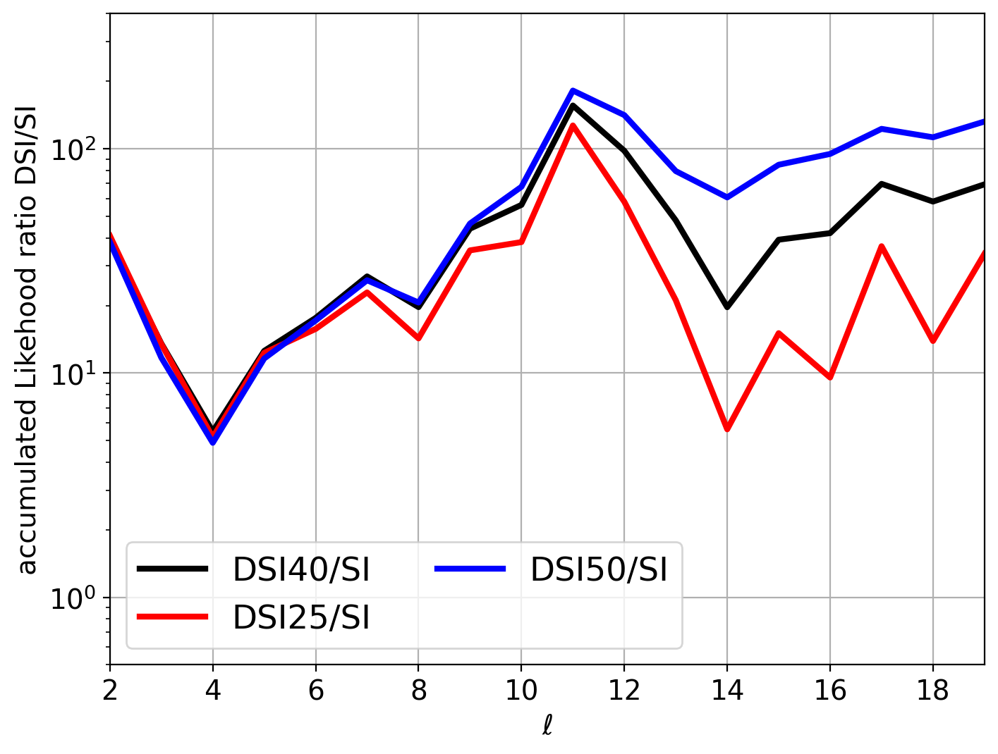
Figure 12: Cumulative likelihood ratio between DSI and SI predictions compared to the CMB data (as a function of the multipole $\ell$). The differnt colors correspond to different values of the cutoff: $\sigma=0.02$ (DSI50, blue) , $0.025$ (DSI40, black) and $0.04$ (DSI25, red).

In the Starobinsky’s formulation Starobinsky:1986fx ; Starobinsky:1994bd the the dynamics of the field fluctuations in Stochastic formalism become Markovian and they are determined by the Langevin equation Starobinsky:1994bd

$$\frac{d\phi}{dN}=-\frac{1}{3H^{2}}\frac{dV}{d\phi}+\sigma aH\hat{\phi}\left(N,\,\textbf{x}\right)\,.$$ (101)

Solving the above Langevin equation even numerically is a very non-trivial tast and this was recently achieved within and also beyond the slow-roll approaximations using the so-called stochastic $\delta N$ formalism (See Fujita:2014tja ; Vennin:2015hra ; Pattison:2019hef ; Mishra:2023lhe ; Jackson:2022unc and references therein). However, it is the non-Markovian system of equations (99) one needs to adopt and solve for DSI to determine the parity asymmetries in the small angular scales or large multipoles. This exercise is entirely non-trivial and is beyond the scope of the present paper. Furthermore, the Parity asymmetries are only significant at large angular scales or small multipoles, therefore, we only look at the infrared modes or course graining modes $k\ll k_{\ast}$ with the value of $\sigma=0.02$. In Table 4 and Fig. 12 we show how the value of $\sigma$ changes the DSI estimates for different values $\sigma=k_{c}/k_{\ast}=0.02,0.025,0.04$. The results only change slightly in this range, but data seems to prefer $\sigma=0.02$, as expected from the above discussion. Therefore, for the first time, we exactly specify what should be the value of $\sigma$ which is most often treated as a free parameter in the stochastic inflation literature Mishra:2023lhe ; Fujita:2014tja . Furthermore, This is an important input to further develop the framework of the stochastic formalism of inflationary fluctuations together with QFT in the inflationary spacetime.

8 Conclusions and outlook

CMB measurements starting from COBE to the latest Planck data have been consistently telling us about the anomalies Schwarz:2015cma at lower multi-poles ($\ell<30$) or large angular scales $\theta>6^{\circ}$. The well-celebrated fit of near scale-invariant power spectrum (16) together with LCDM is perfect only for the physics of angular scales $\theta<1^{\circ}$ or for $\ell>200$. Numerous investigations have been carried out in the last decades with WMAP and Planck data sets to characterize and understand the low-$\ell$ angular power spectrum. The notable challenges have been the low-quadrupole ($C_{2}$), there is more power observed in the odd-multipoles rather than in even-multipoles, the anticorrelation between two-point temperature correlation at the anti-podes of the CMB (i.e, at $\theta\simeq 180^{\circ}$) and the apparent lack of power at $\theta>60^{\circ}$. The common origin of these anomalies has been the major concern for theoretical and observational cosmologists. All these anomalies point to one aspect which is parity that is a discrete symmetry by nature and has nothing to do with the statistically isotropic feature of CMB. Therefore, parity does not seem to conflict with the cosmological principle. By meticulously analyzing the CMB map in the configuration space, we have unveiled a remarkable fact that CMB is parity asymmetric by a significant preference for odd parity. This can be seen by the naked eye in Fig. 2 where the total CMB map (A+S) is very much similar to its antisymmetric counterpart (A). This tells us there are large-scale temperature fluctuations in the CMB (which also means there are large-scale structures in the Universe) that not only look flipped in shape by parity but also asymmetric in amplitude. This picture conveys a clear parity asymmetric feature of CMB and it is calling our attention to understand better the (quantum) physics associated with the early Universe. This is because discrete symmetries and their violations most likely must be related to quantum physics rather than classical physics. History is teaching us about it, it is the understanding and evidence for discrete (a)symmetries such as charge conjugation (${\mathcal{C}}$), Parity (${\mathcal{P}}$), and time reversal (${\mathcal{T}}$) and their combinations ${\mathcal{C}}{\mathcal{P}}$ and ${\mathcal{C}}{\mathcal{P}}{\mathcal{T}}$ have helped us to build quantum field theory and the standard model of particle physics.

Analyzing CMB data is the most tricky aspect, especially since it requires a guiding cue which is, the most plausible theory with the least number of free parameters. In the context of early Universe cosmology, the most plausible theory is advocated to be the near-scale invariant primordial power spectrum (16) together with the LCDM. The power spectrum (16) is widely advocated to be the robust prediction from quantum fluctuations in standard inflation (SI). Since SI+LCDM is the only model that has the least number of parameters, low-$\ell$ CMB data is studied with simulations and sampling variance calculated from SI+LCDM. Naturally, if SI+LCDM not the right model to address the low-$\ell$ anomalies of CMB it is not a correct approach to consider sampling variance from the model. Studies in the past have been strongly suggesting the inconsistency of SI+LCDM at large angular scales and in this paper, we show that the rather remarkable parity asymmetric feature of CMB is quite at odds with SI. Here in this paper, we study a new theory of inflationary quantum fluctuations called Direct-Sum Inflation (DSI) (See Sec. 7) where quantum fluctuations have parity asymmetric time evolution (different time evolution at parity conjugate points in physical space) during inflation. This theory is developed based on an observation that time reversal symmetry would be broken during inflation and corresponding parity should also be broken spontaneously. This framework strongly resonates with what we see in the CMB data i.e., a strong preference for odd parity (See Sec. 3 and Fig. 3).

Given we have two theories of inflationary quantum fluctuations SI and DSI with an equal number of parameters we carefully look into their implications for low-$\ell$ parity asymmetric CMB observables such as Z-parity with its mean distribution and Skewness that measures the temperature anticorrelations at parity conjugate points (See Eqs. (10), (11)), $R^{TT}$ that measures even-odd asymmetry of power in harmonic space (14) and possibilities of finding lower-quadrupole in both models. Since we have two theories with equal parameters, we perform our analysis in two ways, one is we do data simulations (up to $10^{6}$ realizations of CMB sky), and ask the question given the data how probable DSI is in comparison with SI to explain the data. We find robust answers to this question which are summarized in Table. 1 and Figs. 5-8. We also analyze the data by performing the simulations of the models SI and DSI (where we consider the cosmic variance from each model rather than the data), the results of this approach are depicted in Table. 2. In the first approach, we found the DSI is 653 times more probable than SI in explaining the low-quadrupole and $R^{TT}$ given the data. With the Z-parity statistics in configuration space, DSI becomes 54 times more probable than SI, and with both Z-parity and $C_{2}$, DSI is 166 times more favored than SI. In the second approach of finding how probable the models match with data, we still find DSI is 47-55 times more probable than SI. In the whole analysis, the $p-$ values of SI happen to be only ${\mathcal{O}}\left(10^{-4}-10^{-3}\right)$ whereas the DSI stands out to be consistent with data with p-values of ${\mathcal{O}}\left(2-10\right)$. Another notable point here is that the cosmic variance of DSI theory is much closer to the data in comparison with SI which again strongly indicates the power of parity asymmetric inflationary quantum fluctuations. We have found that the lower quadrupole can explain another anomaly associated $S_{1/2}$ (which indicates the lack of correlations in the very large scales $\theta>60^{\circ}$) by a factor of 122 times the p-value found in the SI model. Interestingly the DSI does predict a lower value for quadrupole and it does naturally explain the $S_{1/2}$ anomaly as we can see in Fig. 9. All of this makes the DSI+LCDM the Planck data’s best-fit theory as we can witness in our Fig. 8.

We revisited one of the most discussed anomaly called HPA and its related observables such as the amplitude of DPM (defined in (20)) and $\sigma_{16}^{2}$ which is the variance at $N_{side}=16$. This anomaly has been advocated to challenge the cosmological principle by showcasing evidence for statistical anisotropy in the direction of ecliptic plane (the direction our solar system is oriented) that suggests our place in the Universe as a special one. The way HPA has been shown as significant anomaly in the literature is by doing isotropic Gaussian simulations of SI+LCDM in a specific direction in each realizations. As this introduces a bias, we instead run a million SI+LCDM simulations and looked for HPA in a thousand directions in each realization. Thus, we found evidence for HPA has reduced by the p-value of 2.5% which turned out to be close to the p-value of quadrupolar power in SI (See Table. 3). This establishes a direct connection between HPA and lower-quadrupole. To test this, we studied SI+LCDM model by fixing the quadrupole as low as the data and this has dramatically made the HPA anomaly statistically very insignificant with a p-value of 15%. Furthermore, we have also shown that any dipolar modulation in CMB does not effect the parity measurements such as Z-parity and $R^{TT}$ which proves parity and isotropy are totally different.

In our study, we have only concentrated on parity asymmetric CMB at low-$\ell$, because this is where the major anomalies have been reported from WMAP to Planck. From the mechanism of inflationary quantum fluctuations in DSI, we should expect parity asymmetry at all scales but there are two limitations to explore this in the present paper. The CMB data is not that accurate to tell us about parity asymmetry at smaller scales (large $\ell$). Since the inflationary quantum fluctuations becoming classical is a non-Markovian process, computing parity asymmetry for the smaller scales is completely non-trivial and it requires employing the stochastic formalism and high numerical analysis as we discussed in Sec. 7. We apply a cut-off in wavenumber of inflationary quantum fluctuations $k_{c}=0.02k_{\ast}$ which is the scale that affects the angular power spectrum at low-$\ell$. This determines the so-called coarse gaining modes in stochastic formalism. We greatly expect this would help further to develop the framework and correspondingly the quantum field theory in curved spacetime.

In the coming years, there will be Stage 4 CMB observations which are expected to observe more precisely the polarization of the CMB photons Abazajian:2016yjj . This will add complementary parity information to the $C_{\ell}$ measurements at low-$\ell$, providing a further test to DSI. Furthermore, DSI also predicts parity asymmetry for primordial gravitational wave background Kumar:2022zff which can be extracted from future possible detection of CMB B-modes. Another thing the DSI model predicts is primordial dipole $C_{1}$ at about 50% larger than SI (see Table 4). Thus, the predicted primordial dipole cannot be easily separated from the kinematic dipole and therefore it can translate into a $\simeq 3$Km/s systematic uncertainty in establishing the local motion of comoving observers. This corresponds to $\Delta H_{0}\simeq 3$Km/s/Mpc for the distance ladder calibration 2021ApJ…908L…6R of $H_{0}$ at 1 Mpc distance. Further work is needed to address the possible implications of such uncertainty. Given the Hubble tension of late-time cosmology has been gaining significant attention in recent years DiValentino:2021izs , it would indeed be worth investigating the effect of DSI’s primordial dipole in the local expansion measurements.

Finding a signature for the quantum mechanical nature of gravity (i.e., quantum gravity) is the most vital key to understanding early Universe and Black Hole physics and also to build a consistent ultraviolet complete theory of quantum gravity towards the Planck scales. What else would be the most important signature for quantum gravity than a parity asymmetric CMB emerging from primordial quantum fluctuations in the early Universe? The Direct-Sum-Inflation resolves the conundrum between gravity and quantum mechanics by separating the concept of time in GR with the concept of time for quantum fluctuations in curved spacetime. In the DSI, the clock in the expanding FLRW Universe would be the scale factor and the quantum-mechanical (parametric) time allows the quantum fields to respect the (a)symmetries of background spacetime. The evidence we found for DSI in this paper is only the first step in further exploring the role of gravity and quantum mechanics at the spacetime horizons.

Appendix A Making parity-conjugate CMB maps with Healpix

In the HEALPX (hp) format a map is just an ordered 1D array of ($\Delta T$) numbers map[pix] where pix is an index array that runs from $0$ to Npix-1. The number of pixels Npix depends only on the map resolution NSIDE: Npix = 12 NSIDE*NSIDE. The angular spherical coordinates (t,p)$=(\theta,\varphi)$ of each pixel is just given by the order in the index array pix with a transformation (i.e. the HEALPX pixelization scheme) that only depends on NSIDE: t, p = hp.pix2ang(nside,pix). To apply a parity transformation on a sphere with HEALPX we follow 2 simple steps:

1. Apply the parity transformation $(\theta,\varphi)\implies(\pi-\theta,\varphi+\pi)$ and get the corresponding pixel ${\mathcal{P}}$ conjugate array pix_mirror:
   pix_mirror = hp.ang2pix(nside, $\pi$- t, p + $\pi$)

2. The spherical ${\mathcal{P}}$ conjugate map, map_mirror, is then just given by:
   

   map_mirror[pix_mirror] = $\pm$ map[pix]

where the $\pm$ signs correspond to the odd and even parities. To illustrate this transformation with a familiar image we show in Fig. 13 the different parity transformations of the Earth elevation map. The maps show that Earth’s elevation shows a preferred odd parity, at least at the level of large continents, except the polar caps, which are even.

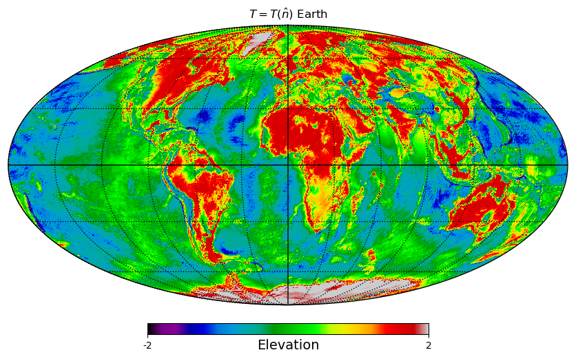
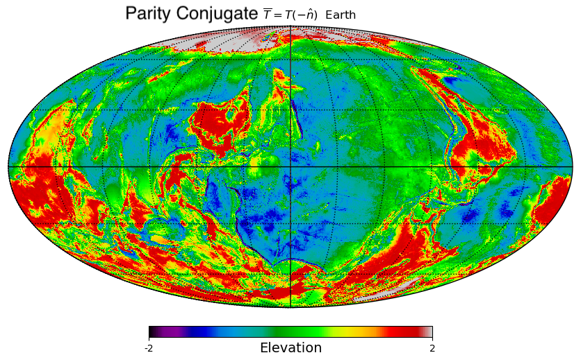
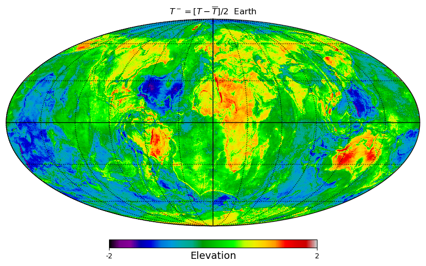
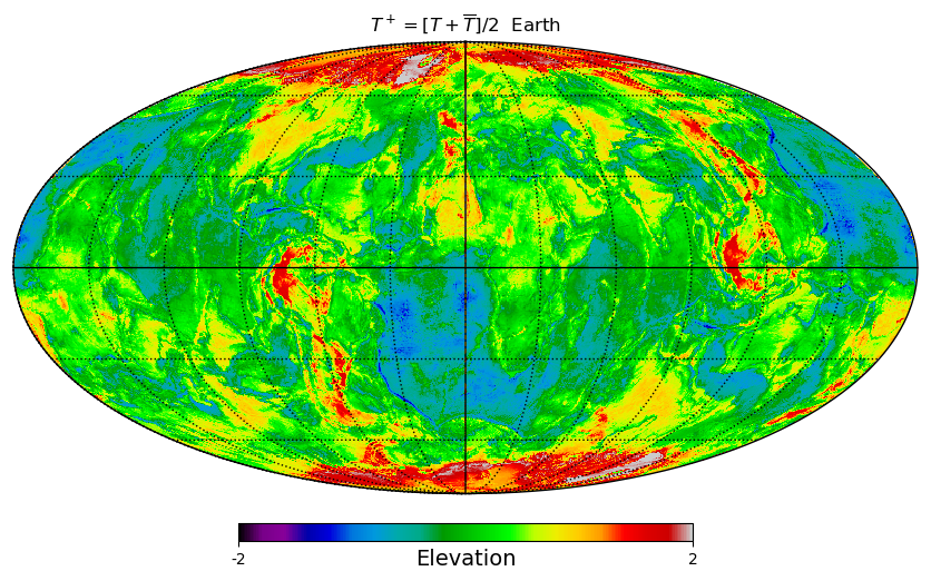
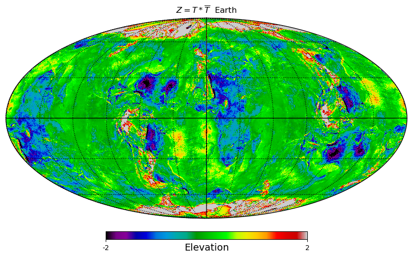
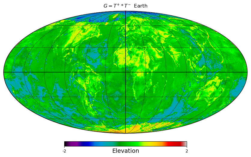
Figure 13: In these Mollview projections, we compare the antisymmetric ($T^{-}$ odd parity, middle left) and symmetric ($T^{+}$ even parity, middle right) decomposition of the Earth elevation map (top left). The Earth ${\mathcal{P}}$ conjugate image $\overline{T}(\hat{n})=T(-\hat{n})$ (top right) indicates where to find the antipodes of the original map. The odd parity map shows the locations where the antipodes of a given elevated continent match a deep ocean depression (like Australia), while the even parity matches regions with similar elevation in the antipodes (like the polar caps or Europe-New Zeland). This can also be seen in the $Z=T*\overline{T}$ map which shows blue for odd and red for even continents. The cross-map $G=T^{+}*T^{-}$ is predominantly noise close to zero, except in the polar caps.

Appendix B Sampling variance and Non-Gaussian distribution of errors

Fig. 5 shows a comparison of the measured $C_{\ell}$ for the lower multipoles (i.e. larger scales) in the CMB temperature maps against the corresponding estimates in simulated maps that will be described below. We also show the diagonal $\chi^{2}$ values of the data and models, given the simulations. The $\chi^{2}$ values seem to prefer the odd-parity model (DSI+LCDM) over the standard inflation (SI+LCDM) model. But such a simple interpretation should be taken with caution for several reasons. First of all, the errorbars (or covariance matrix) are dominated by sampling variance and therefore depend on the model assumption. This can be easily seen in the figure as the shaded region from the simulations is quite different for the SI model (top left), for the data (top right), or the odd-parity models (bottom panels). Second, the covariance matrix is not quite diagonal (because of the map masking). Third, for SI the large $\chi^{2}$ values are dominated by the low quadrupole $C_{2}$ in the data. This is a prediction of the odd parity model, but could also originate from a break in the primordial power spectrum, unrelated to parity symmetry. Fourth, the distribution of $C_{\ell}$ values is not Gaussian (e.g. see Bond2000 and references therein). This is illustrated in Fig. 14. More generally, when doing such $\chi^{2}$ we are testing different aspects of the model (like gaussianity, scale-invariant, or global isotropy) and not just directly parity.

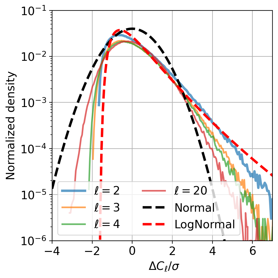
Figure 14: Left: Distribution of normalized variations $\delta_{\ell}\equiv\Delta C_{\ell}/\sigma$ for the lower order multipoles ($\ell=2-20$) in $10^{6}$ masked map realizations of the measured $C_{\ell}$ in the Planck SMICA_m map, compared to the Normal distribution (dashed black). The distribution is non-Gaussian which makes a simple $\chi^{2}$ test hard to interpret. For example, a $\simeq+4\sigma$ fluctuation in $C_{2}$ is about $10^{2}$ more likely in the actual data than in the Gaussian prediction, while $\simeq-2\sigma$ fluctuations is almost $10^{2}$ times less likely. The Log-Normal distribution (dashed red) gives a better approximation for $C_{2}$, but far from perfect. Right: normalized covariance matrix $Cov[\ell,\ell^{\prime}]=<\delta_{\ell}\delta_{\ell^{\prime}}>$ between $\delta_{\ell}$ in two different multipoles $[\ell,\ell^{\prime}]$. The cross-correlation Pearson coefficients are always below $15\%$.

Fig. 5 suggests that the octopole $C_{3}$ aligns more closely with SI than with DSI. While this observation holds true, the difference is less pronounced compared to $C_{2}$. The p-value of $C_{3}$ in DSI is approximately $9-10\%$, which is 3 times smaller than the $28\%$ for SI. This could mean that there is something else going on the largest scales: $\ell=2-3$ (i.e. lack of power on scales $\theta>60^{\circ}$). However, a low $C_{3}$ remains a plausible random fluctuation given the range of multipole draws explored within $\ell<20$. The reason for the contrast in significance between $C_{2}$ and $C_{3}$ lies in the fact that sampling variance errors in $C_{\ell}$ are directly proportional to $C_{\ell}$:

$$\Delta C_{\ell}=\frac{C_{\ell}}{\sqrt{(2\ell+1)f_{sky}}}.$$ (102)

An increase in $C_{\ell}$ (occurring for odd $\ell$ under odd-parity) entails larger sampling errors compared to a decrease, as observed in the case of $C_{2}$. Consequently, deviations in even multipoles are more statistically significant than those in even ones. In addition, the lower $\ell$ multipoles have a more pronounced non-Gaussian distribution of errors.

We can avoid some of these complications by just focusing on the alternating even-odd oscillation in the $C_{\ell}$ multipoles, which is the distinct feature of parity (e.g. see (13)). Such an approach has already been reported in several analyses (see 2005PhRvD..72j1302L ; Kim:2012hf ; Muir:2018hjv ; Jones:2023ncn and references therein). We will use $R^{TT}$ defined in (14) (e.g. see Muir:2018hjv and references): Here, we will set $\ell_{max}=20$, motivated by our predictions. We have checked that our results remain similar for $\ell_{max}=22,27$, and $30$ which are the other values that have been used in the literature. For SI we expect $R^{TT}\simeq 1$ because the fluctuations have no defined parity. For the Planck 2018 masked SMICA map, Jones:2023ncn finds $R^{TT}=0.79$ for $\ell_{max}=27$ with a p-value for SI of $\simeq 10^{-2}$ (this is the probability that a randomly generated SI realization produces a value of $R^{TT}$ as extreme as—in this case, lower than—the observed data). This result indicates a pronounced antisymmetric component (20% larger odd parity) in the data.

Appendix C CMB simulations

Fig. 15 displays the version of the common mask employed for the parity $Z$ maps. This ${\mathcal{P}}$ conjugate mask results from combining the common mask with its ${\mathcal{P}}$ conjugate image (see Appendix §A). Generally, our conclusions remain consistent across different component separations or masks, though the specific numerical values may differ. Unless specified otherwise, results will be presented for SMIC_m. Additionally, this is the default model simulated for estimating data error bars.

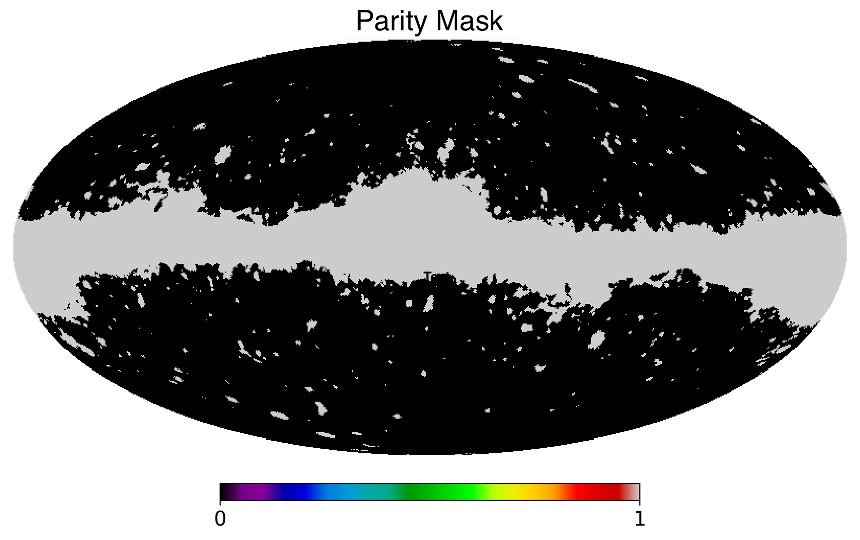
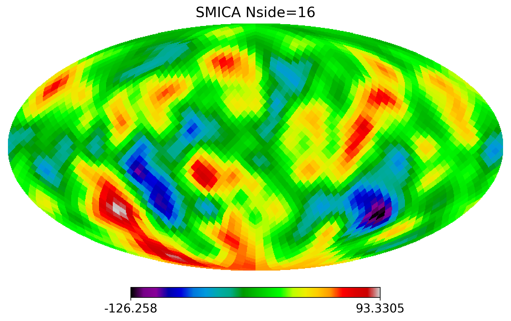
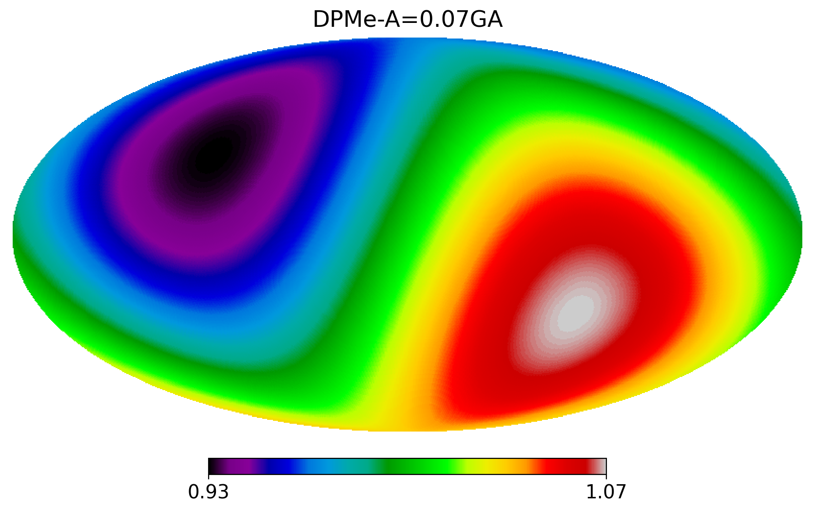
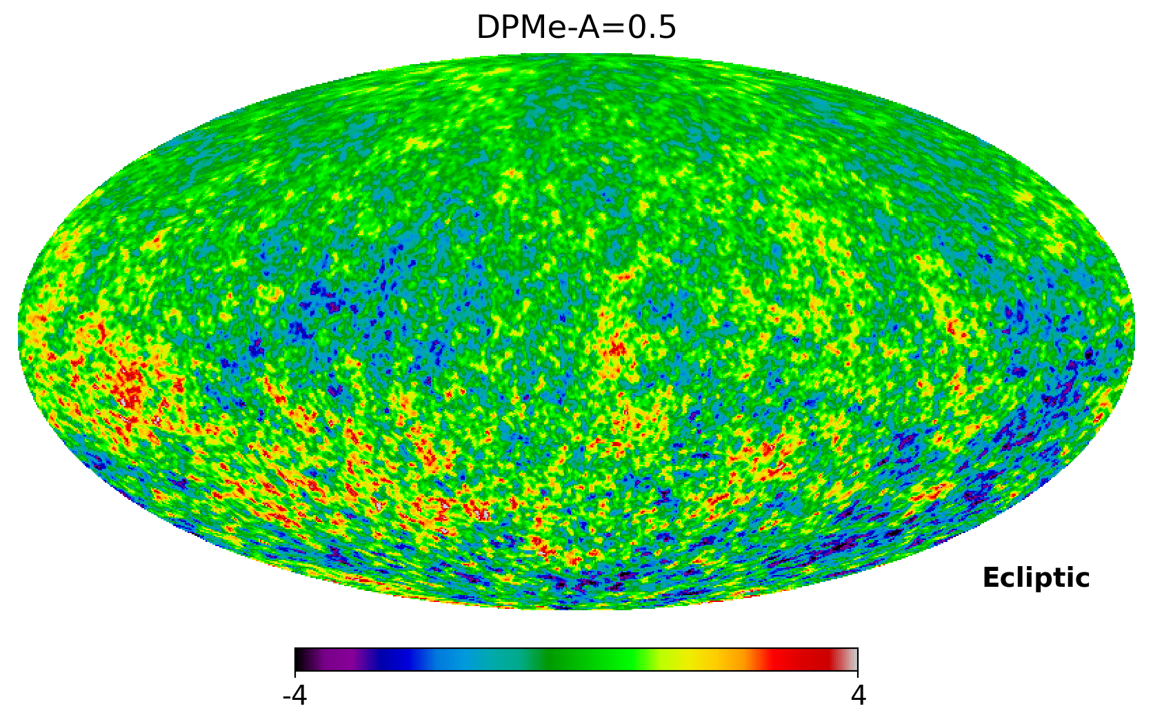
Figure 15: Top Left: ${\mathcal{P}}$ conjugate product image of the Planck common mask ($77.9\%$ of the sky), which is needed for the $Z$ map masking. This $Z$ masked map covers only 74% of the sky. Top Right: Planck 2018 (SMICA) maps in Ecliptic coordinates with $N_{side}=16$ and smoothing of $10.5^{\circ}$. This clearly shows less structure in the North Eclictic pole and is used to estimate the $\sigma_{16}^{2}$ HPA anomaly. Bottom Left: A dipole modulation in (20) with $A=0.07$ (shown in Galactic coordinates) pointing in the direction of the South Ecliptic pole. Bottom Right: A LCDM Gaussian realization of the dipolar anisotropy modulation (DPM) model in (20) with $A=0.5$ in Ecliptic coordinates (dipole is negative on the North Ecliptic Cap). Note that $A=0.5$ is much larger than the value $A=0.07$ allowed by the Planck data and is only used here to state the separation between isotropy and parity symmetries.

We generate Gaussian simulations based on the Planck 2018 best-fit LCDM model using the Helapix routine symfast with $N_{side}=2048$. We introduce instrumental noise and a $\theta_{B}=5$ arcmin Full Width at Half Maximum (FWHM) Gaussian beam. The Planck 2018 best fit is predominantly influenced by $\ell>40$, where the signal-to-noise is more significant, and the Baryon Acoustic Oscillation (BAO) peaks are prominent. The top left panel of Fig. 16 illustrates this fit in blue.

To assess the accuracy of our simulation, we simulate the blue line with symfast (smoothed with a $\theta_{B}=5$ arcmin beam) and measure the $C_{\ell}$ back from the simulated map using anafast. The result is represented by the gray line labeled ’sim test’ in the figure. The difference between gray and blue lines is due to the instrumental noise and instrumental beam smoothing. The gray line is further compared to the same direct measurement of $C_{\ell}$ in the Planck SMIC_m maps (in red), post-application of the mask, and division by $f{sky}$. The two outputs exhibit a remarkable overlap for all multipoles, essentially lying on top of each other. This test emphasizes that our simulations faithfully reproduce the intended models.

Since our focus is on studying the largest scales, there’s no necessity to work with such a relatively large resolution of $N_{side}=2048$. Consequently, we downsampled the maps to $N_{side}=256,128,$ or $64$ and applied smoothing with $\theta_{S}=0.5^{\circ},1^{\circ},$ or $2^{\circ}$. These processes were also applied to the Planck maps for consistency.

The instrumental noise exhibits minimal impact on the smoothed $N_{side}<256$ maps, particularly at the low multipoles. This was previously demonstrated by Muir:2018hjv , who conducted a comparison between simulations incorporating realistic noise (derived from FFP8.1 Planck public simulations) and simpler symfast simulations. The findings indicated that both approaches yield very similar statistics for CMB anomalies at $\ell<30$.

To focus on the parity symmetry, we normalize $\Delta T$ in the low-resolution maps by $\sigma_{T}$, defined as the root mean square (RMS) of the temperature map: $\sigma_{T}=\sqrt{\langle\Delta T^{2}\rangle}$. In practice, we estimate $\sigma_{T}$ by determining the 68% percentile width of the 1-point $\Delta T$ probability distribution function. This approach is more robust in the presence of outliers or artifacts.

When estimating $\sigma_{T}$, it is crucial to utilize only the data outside the mask. This is because values within the mask possess different noise properties, and we want to avoid introducing such noise into the CMB signal. By doing so, the results become less sensitive to resolution or noise at the pixel level. The resulting pipeline statistics prove to be quite robust, yielding very similar results and conclusions across different resolutions. For simplicity, we default to presenting results for $\theta_{S}=2^{\circ}$ and $N_{side}=64$.

The parity measurements yield very similar results whether one degrades higher resolution simulations from $N_{side}=2048$ to lower resolutions (e.g., $N_{side}=64$) or directly simulate CMB maps at the lower resolution without any instrumental noise. The efficiency gained from the latter approach adds practicality to the methodology.

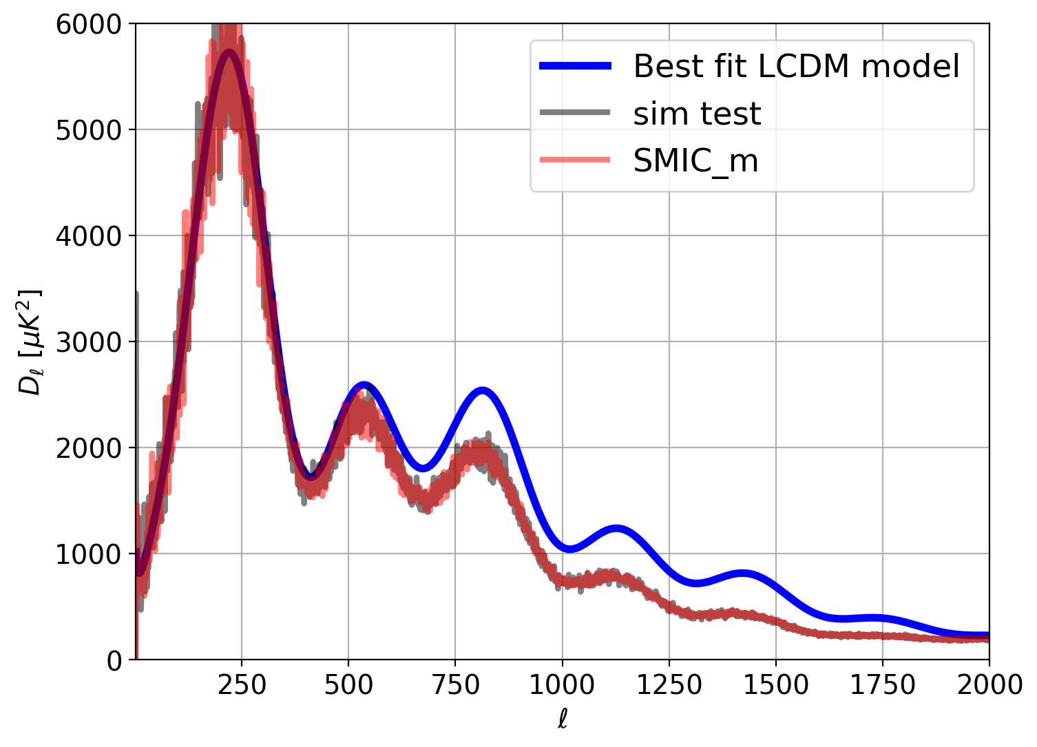
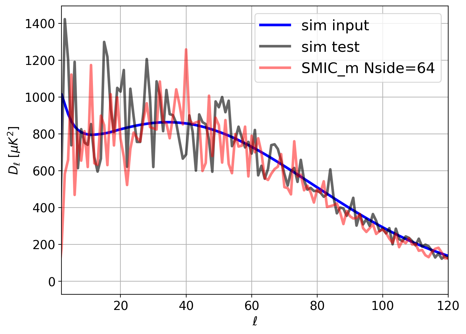
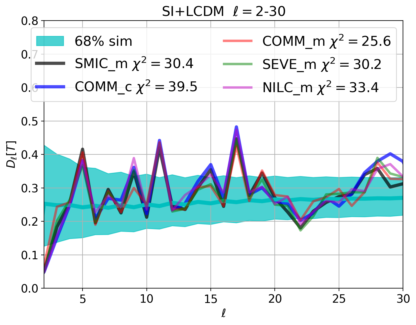
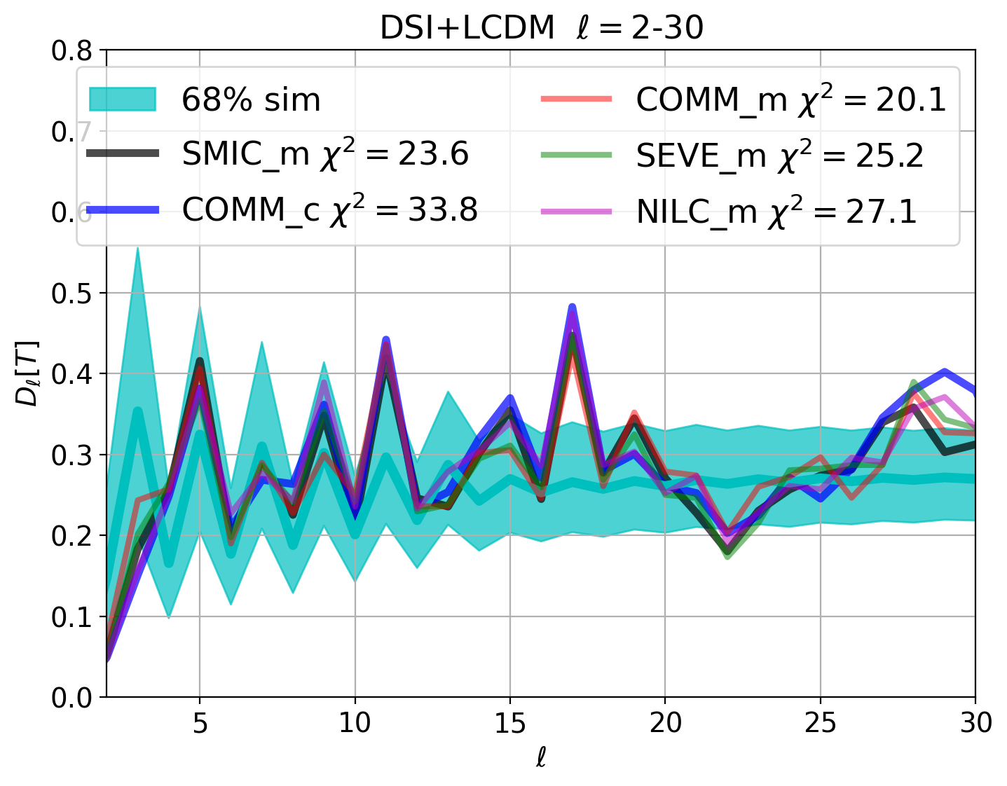
Figure 16: Top left : Planck 2018 best-fit LCDM model power spectrum $C_{\ell}$ (blue), which is the input for our simulations. In gray we show the measured $C_{\ell}$ from the simulation test with $N_{side}=2048$ and $r_{beam}=5^{\prime}$, as in the Planck maps. It overlaps very well with the measurements in the Planck SMIC_m map (shown in red). The differences for $\ell>500$ between the raw input and the measurements are due to the instrumental beam smoothing, noise, and masking. Top Right: Zoom in on the lower multipoles measured after degrading the maps to $N_{side}=65$ (with $r_{beam}=2^{\circ}$ Gaussian beam). This is the default resolution in our parity analysis. Bottom Panels: Shaded (cyan) region corresponds to 68% range of $C_{\ell}$ values around the mean from $10^{6}$ simulations in SI+LCDM (left) and DSI+LCDM (right). These models are compared to $C_{\ell}$ measured in the different Planck 2018 maps. We have degraded and smoothed the original maps and simulations from $N_{side}=2048$ to $N_{side}=64$ and normalized them to unit variance.

We have checked that the smoothed normalized low-resolution maps (with $N_{side}=64$) also have the same average power spectrum $C_{\ell}$ as the corresponding data. This is shown in the right panel of Fig. 16. The bottom panels of Fig. 16 show a zoom-in around the lower multipoles.

In Fig. 17, we further test our simulations by demonstrating that both Planck data and simulations exhibit Gaussian 1-point statistics with unit variance (as the temperature is normalized to $\Delta T/\sigma_{T}$). While there is a small negative skewness in the Planck maps, it remains consistent with zero at the 1$\sigma$ level, contingent on the component separation map used. The most noticeable discrepancy (still within $2\sigma$) arises from the COMM_m map, which has the smallest mask. When utilizing the common mask (labeled COMM_c in the figure), the skewness in COMM_m reduces to half its value. The skewness becomes more pronounced (deviating from zero) when the mask is not applied (right panel). This is an artifact. Moving forward, we’ll exclusively present results outside the masked region.

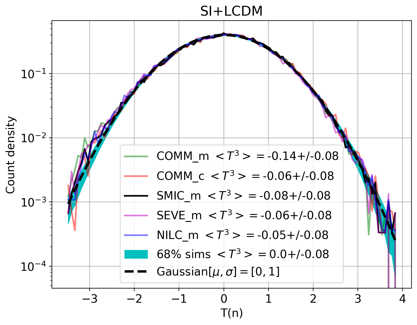
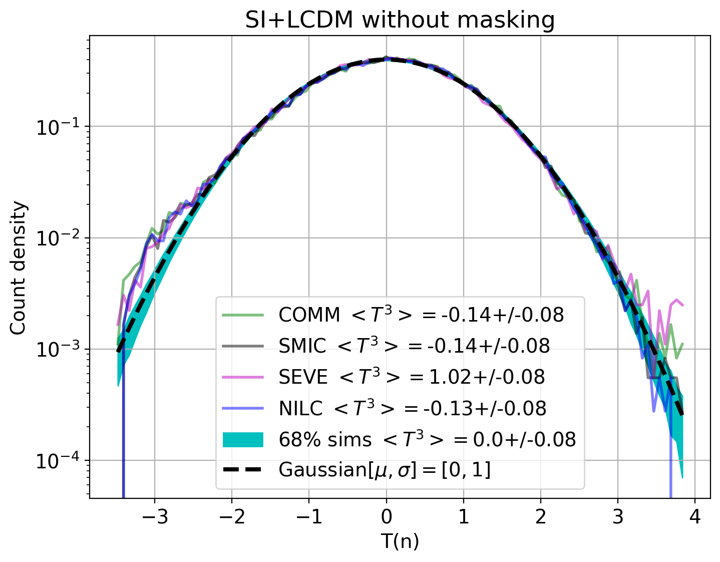
Figure 17: Test of Gaussianity in the CMB maps and simulations, with (left) and without (right) mask.

Simulating the SI+LCDM-C2 model involves repeating the same SI simulation, with the only modification being the fixation of the quadrupole $C_{2}$ to the value measured in the Planck SMICA masked map (SMIC_m). Comparable results are observed for the other component separations.

To simulate the DPM model described in (20), the process begins by generating a fixed dipole using Healpix hpt.dipole_pdf with an amplitude $A=0.07$ and oriented toward the South Ecliptic pole (to emphasize power in the South). An extreme case with $A=0.5$ was also explored. This fixed dipole is then multiplied by each of the LCDM realizations. An illustrative example with $A=0.5$ is presented in the left panel of the bottom right of Fig. 15, showcasing a visible dipolar anisotropy.

To simulate the DSI we add a new component to the SI best-fit (+LCDM) model:

$$C^{DSI}_{\ell}=C^{SI}_{\ell}\left(1\pm\Delta{\mathcal{C}}_{\ell}\right)$$ (103)

where $+$ is for odd-$\ell$ and $-$ stands for even-$\ell$. The $\Delta{\mathcal{C}}_{\ell}$ is given by

$$\Delta{\mathcal{C}}_{\ell}=\frac{1}{C_{\ell}^{SI}}\int_{0}^{k_{c}}\frac{dk}{k}A_{s}\left(\frac{k}{k_{s}}\right)^{n_{s}-1}j_{\ell}^{2}\left(\frac{k}{k_{s}}\right)\left(\Delta{\mathcal{P}}_{v}\right)$$ (104)

where $\Delta{\mathcal{P}}_{v}$ can be read from (18) and

$$C_{\ell}^{SI}=\int_{0}^{\infty}\frac{dk}{k}A_{s}\left(\frac{k}{k_{s}}\right)^{n_{s}-1}j_{\ell}^{2}\left(\frac{k}{k_{s}}\right)$$ (105)

Since (104) is the ratio, the LCDM transfer function’s contribution cancels out in the numerator and the denominator. This modification (103) oscillates as shown in bottom panels of Fig. 16 and Table 4.

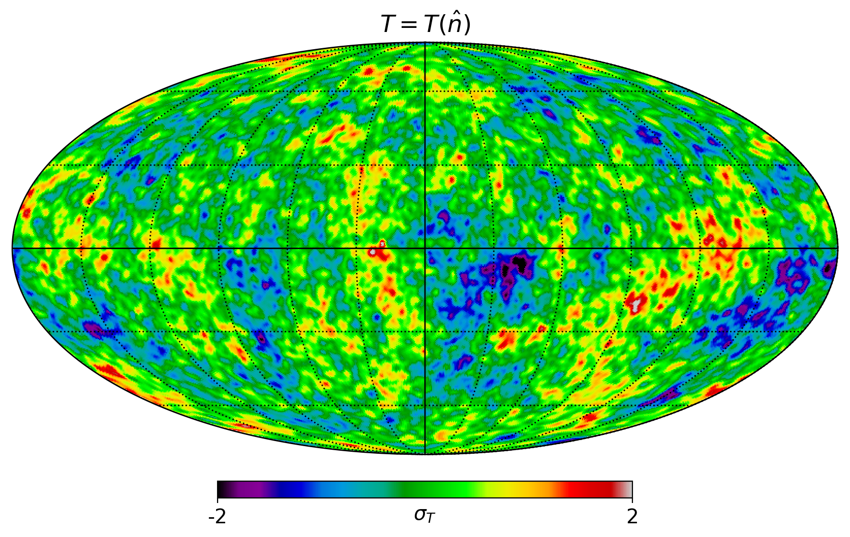
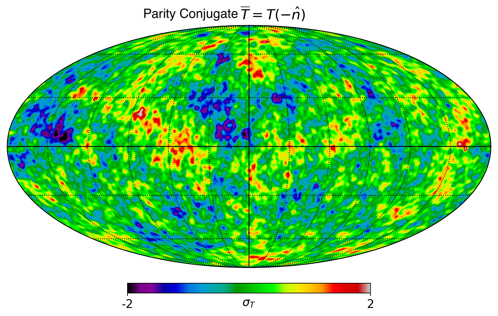
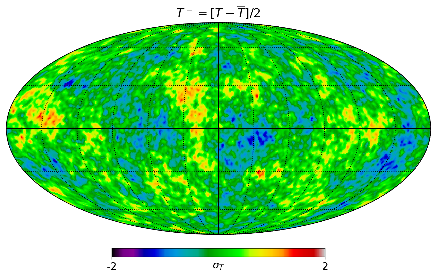
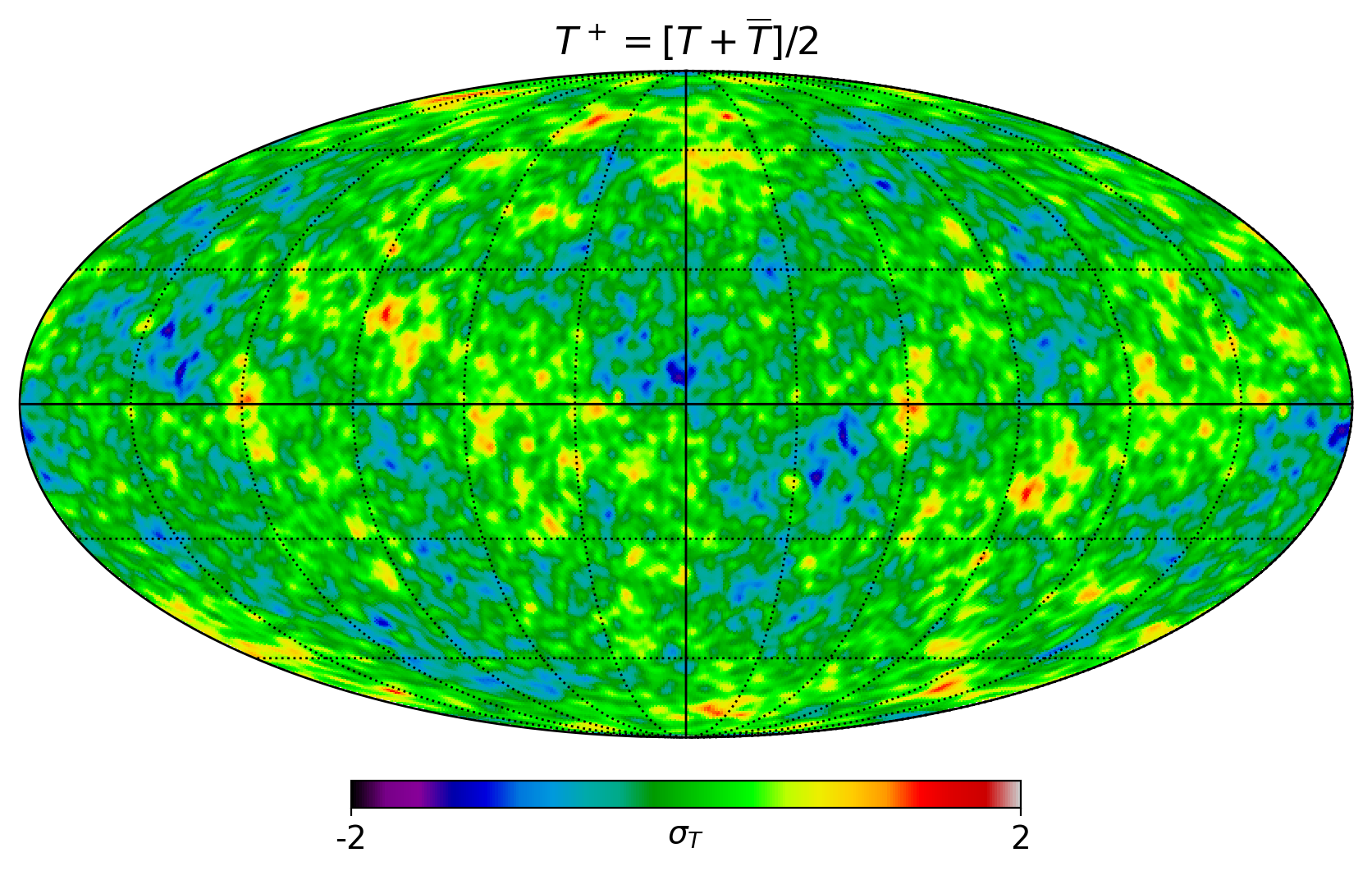
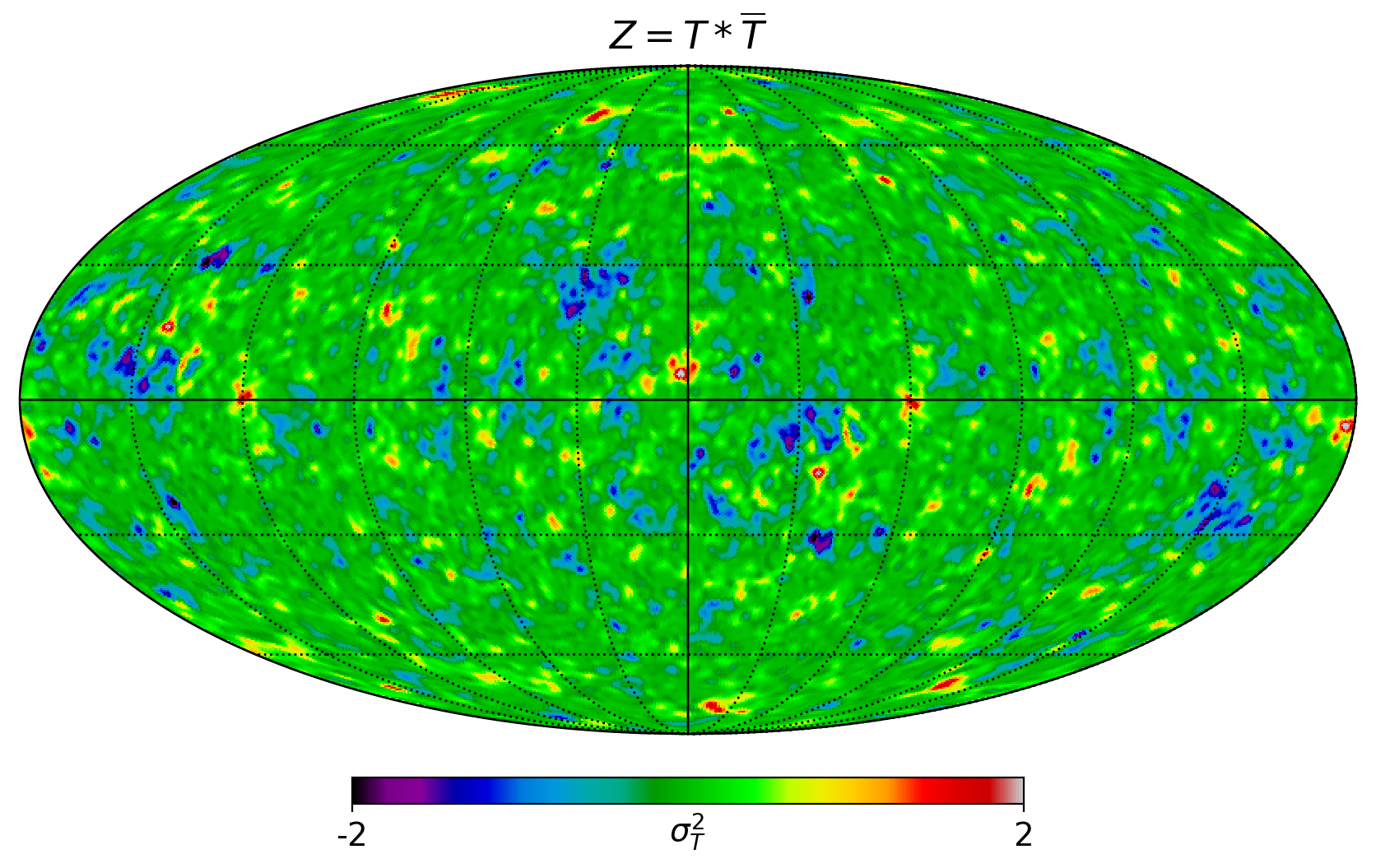
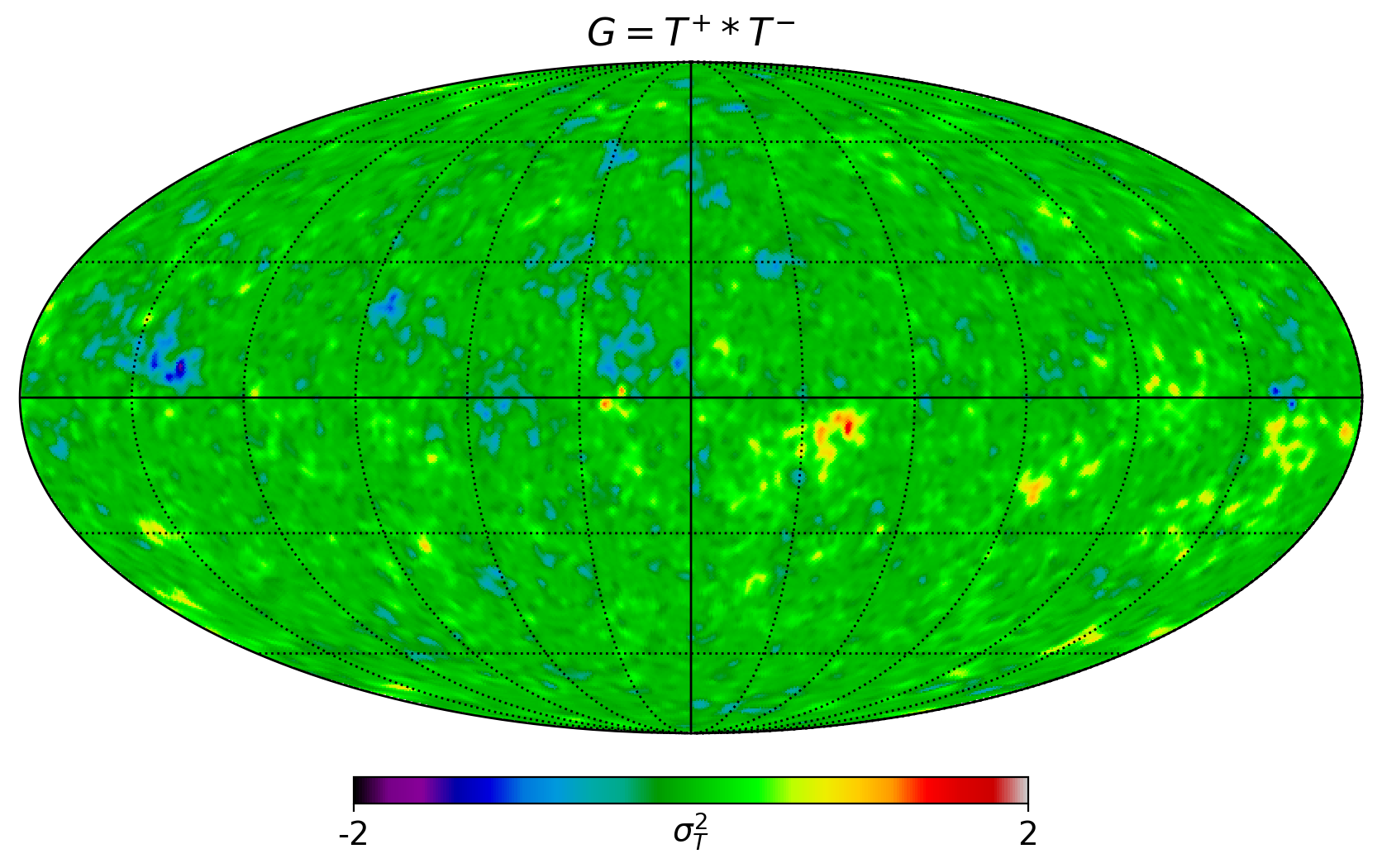
Figure 18: In these Mollview projections, we compare the antisymmetric ($T^{-}$ odd parity, middle left) and symmetric ($T^{+}$ even parity, middle right) decompositions of the Planck 2018 map (SMICA, top left). Furthermore, we showcase its ${\mathcal{P}}$ conjugate image $\overline{T}(\hat{n})=T(-\hat{n})$ (top right). The odd parity map resembles the original more closely than the even parity counterpart. This can also be seen in the $Z=T*\overline{T}$ map which is characterized by a prevalence of negative (blue) values. The cross-map $G=T^{+}*T^{-}$ is predominantly near zero, except in the proximity of the cold structure close to the Galactic Center.

Appendix D Homgeneity Index and lack of correlations at $\theta>60^{\circ}$

Both (2) and (8) assume local statistical isotropy. But even when a fluctuating field ${\mathcal{T}}(\hat{n})$ is found to be locally isotropic, we can also test if, on the largest scales, the amplitude of such fluctuations tend towards global isotropy, which we will also call Homogeneity (to distinguish it from the local isotropy, but not to be confused with 3D translation invariance) and will be better defined in the next paragraph. COBE COBEw2 , WMAP (Bennett-wmap ; Bennett-wmap ; gazta2003 ) and latter Planck (Planck:2013lks ), found an anomalous (lack of) amplitude of large-scale fluctuations in the CMB sky (see our Fig. 9). The integrated value of the square 2-point temperature correlation $S_{1/2}$ for separations above $\theta>60^{\circ}$ has been used as a measure of how much power there is on such large scales Bennett-wmap :

$$S_{1/2}=\int_{-1}^{1/2}w^{2}[\theta]d(\cos{\theta}).$$ (106)

This additional test of (global) isotropy has no directional component. Because $S_{1/2}$ is quadratic in $w$ (and in $C_{\ell}$) , it results in a non-linear response to rare statistics which can be hard to interpret.

A better measurement of such global isotropy is given by the Homogeneity index $\mathcal{H}$ (Camacho-Quevedo:2021bvt ). This is a Hausdorff or fractal dimension Mandelbrot ; Mandel , which is a rigorous way to characterize geometrical irregularities and chaos in Nature. The idea of the homogeneity index, $\mathcal{H}$, is to test if the (2D) metric associated with a given map of fluctuations tends towards a homogeneous (2D) metric on the largest scales. The index $\mathcal{H}$ is independent of the amplitude of fluctuations. It only depends on the slope (how the amplitude of fluctuations changes as we change the angular separation $\theta$):

$$\mathcal{H}(\theta)=2\frac{d\ln{\mathcal{P}}}{d\ln{\Omega}}\quad;\quad\mathcal{P}=\frac{1}{1-\cos{\theta}}\int_{0}^{\theta}\left(1+w[\theta]\right)d(\cos{\theta})$$ (107)

For a global isotropic (i.e. homogeneous) metric we expect $\mathcal{H}\simeq 0$ on the largest scales. Standard Primordial Inflation (SI) is near scale-invariant (16) and therefore has $\mathcal{H}\neq 0$ also on the largest scales. This is at high odds with the actual CMB measurements (Camacho-Quevedo:2021bvt ), which shows $\mathcal{H}\simeq 0$ for $\theta>60^{\circ}$, which corresponds to $\ell<4$ (i.e. a lower than expected quadrupole $C_{2}$ and octopole $C_{3}$). We have checked here that the p-values of $\mathcal{H}$ at $\theta=180^{\circ}$ follow a very similar trend to the ones of $Z^{1}$ shown in Table 1-2, which confirms the odd parity in the 2-point function using a more robust measurement of global isotropy.

Appendix E Visual comparison of the models to data

In this section, we’ll demonstrate how one can easily discern odd parity with a simple visual inspection of the right CMB maps. In the upper-left panel of Figure 18, we present the Cosmic Microwave Background (CMB) temperature, denoted as $T=T(\hat{n})$, extracted from the Planck map using the SMICA component separation method.

In the top-right panel, we compare it to its spherical ${\mathcal{P}}$ conjugate image, denoted as $\bar{T}=T(-\hat{n})$. Moving to the middle panels, we explore the odd and even parity components: $T^{-}=(T-\bar{T})/2$ and $T^{+}=(T+\bar{T})/2$. Further, we examine their multiplication, represented by $Z=T*\bar{T}$ and $G=T^{+}*T^{-}$ in the bottom panels. All these maps are presented in Galactic coordinates. For the corresponding maps in Ecliptic coordinates, refer to Figure 19.

If you squint at the middle maps, you’ll observe that the original $T$ map bears a closer resemblance to the odd $T^{-}$ component than the even $T^{+}$ component. This holds in both coordinate systems. This visual impression agrees very well with the more quantitative split $w^{+}/w^{-}$ shown for $w(\theta)$ in the left panel of Fig. 9 or the even/odd oscillations of $C_{\ell}$ in Fig. 5. Another indicator is that the $Z$ map is predominantly dominated by blue (i.e., negative) values, which matches with the asymmetry evident in $P(Z)$ distribution in Fig. 6.

In comparison, the corresponding maps for SI realization, as illustrated in Fig. 20, exhibit no discernible preference for even or odd parity. These visual observations can be further contrasted with the DSI maps in Fig. 21, which exhibit similar odd parity features as observed in the Planck maps.

In contrast with the other maps, the maps of $G=T^{+}*T^{-}$ (bottom right corner of each figure) are in all cases consistent with white noise. This indicates that the odd and even components are not coupled, which is what we expect out of Gaussian statistics. This characteristic arises from the independence of each multipole, and it trivially extends to the independence between even and odd multipoles.

Exceptions to this rule are observed in the form of rare bright hot spots. These spots, appearing as cold spots in the antipodal opposite direction due to ${\mathcal{P}}$ conjugate symmetry construction, might signify rare events or could be artifacts caused by galactic or foreground contamination in some of the maps. Rare events are inevitable due to the finite size of the observable sky realization. At any resolution, this realization has a maximum number of unique draw values, with the extreme values being labeled as rare events or anomalies, as discussed in Creswell:2021eqi . In our analysis, we mitigate the impact of these rare events by employing a 4-sigma clipping to the maps before conducting statistical measurements. This approach allows us to distinctly separate the parity study from the interpretation of rare events.

The very extreme $A=0.5$ DPM model in Figure 22, shows a dipolar component in the $G$ map. Despite such strong anisotropy, the $Z$ map and the parity statistics, e.g. $P(Z)$ or $R^{TT}$, show no preference for parity (see Table. 2). This is a clear demonstration of how the $P(Z)$ distribution allows us to separate isotropy from parity.

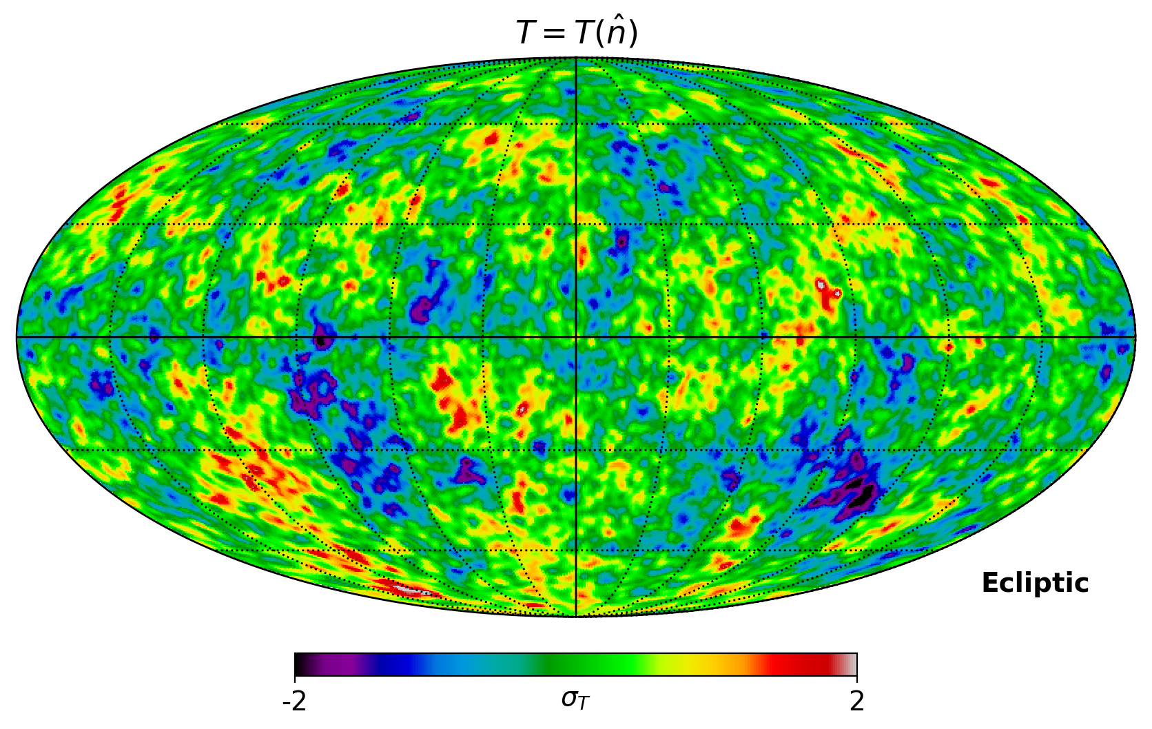
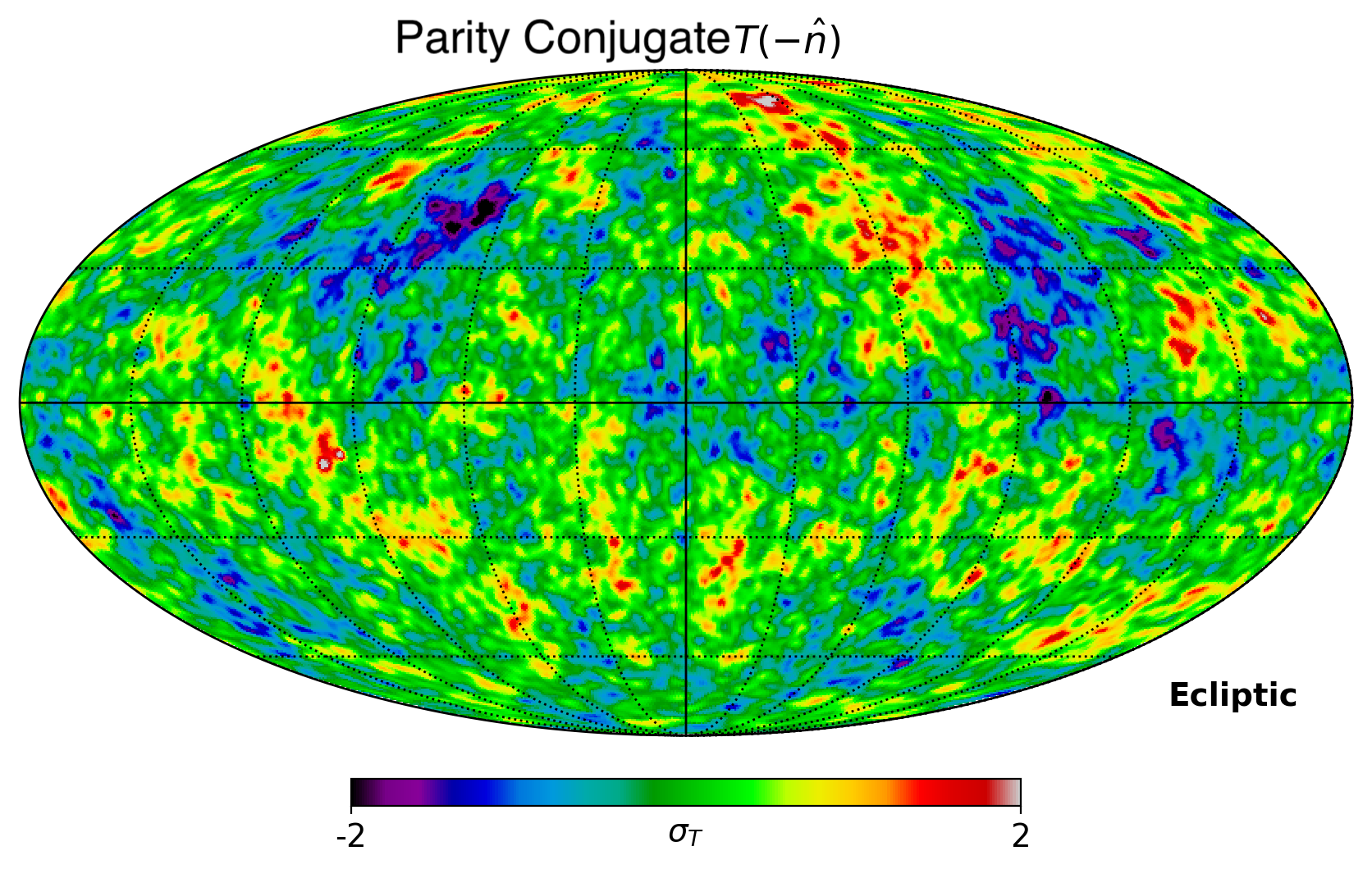
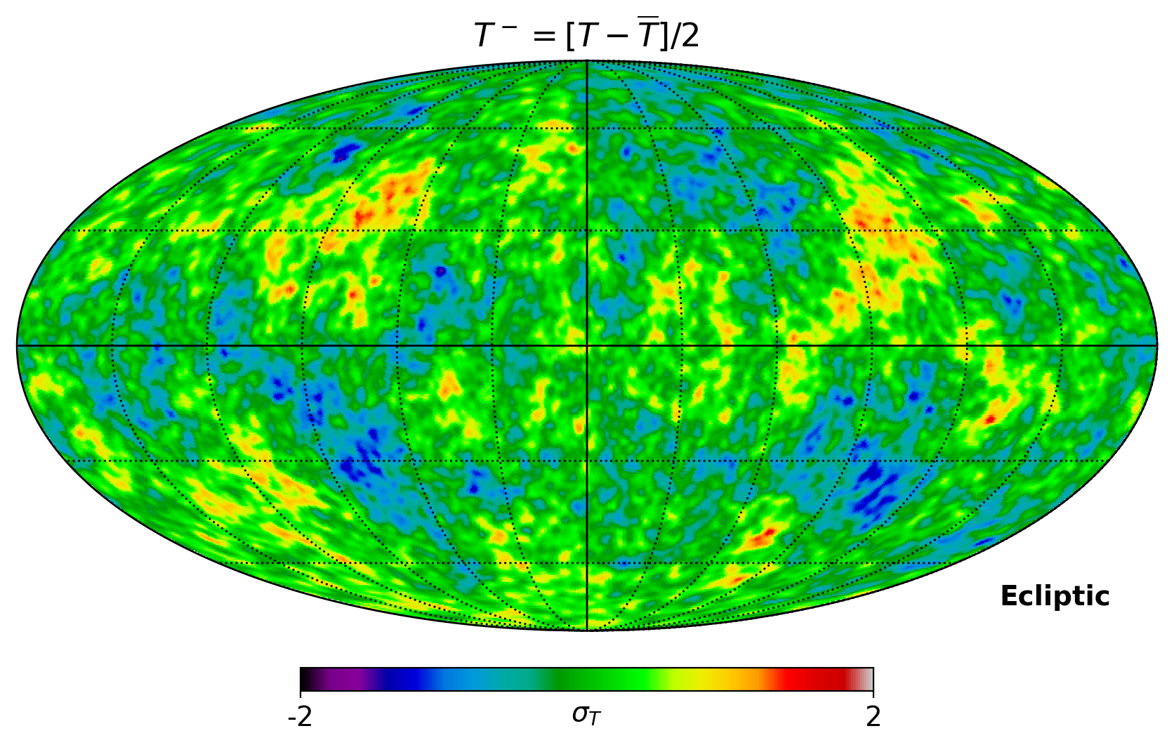
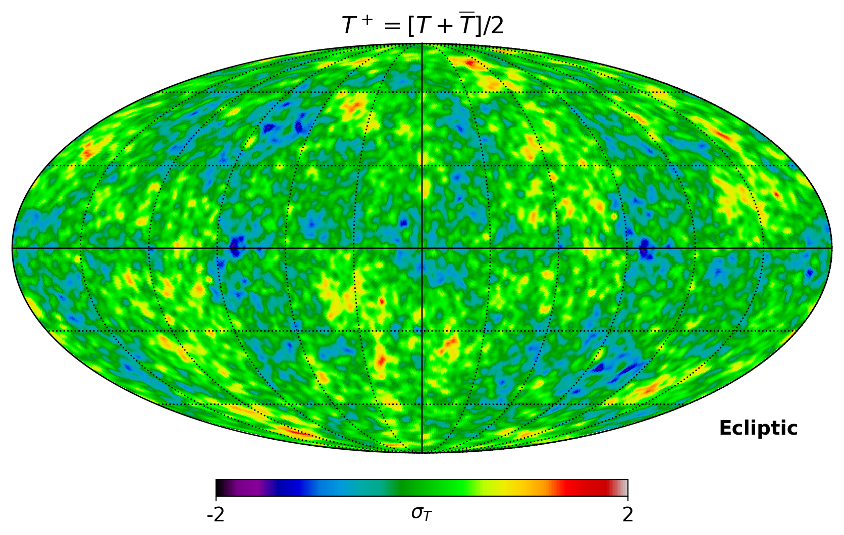
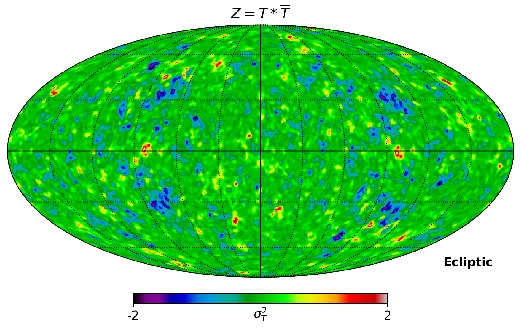
Figure 19: Same as Fig. 18 in Ecliptic coordinates, where there is the maximal hemispherical power difference.

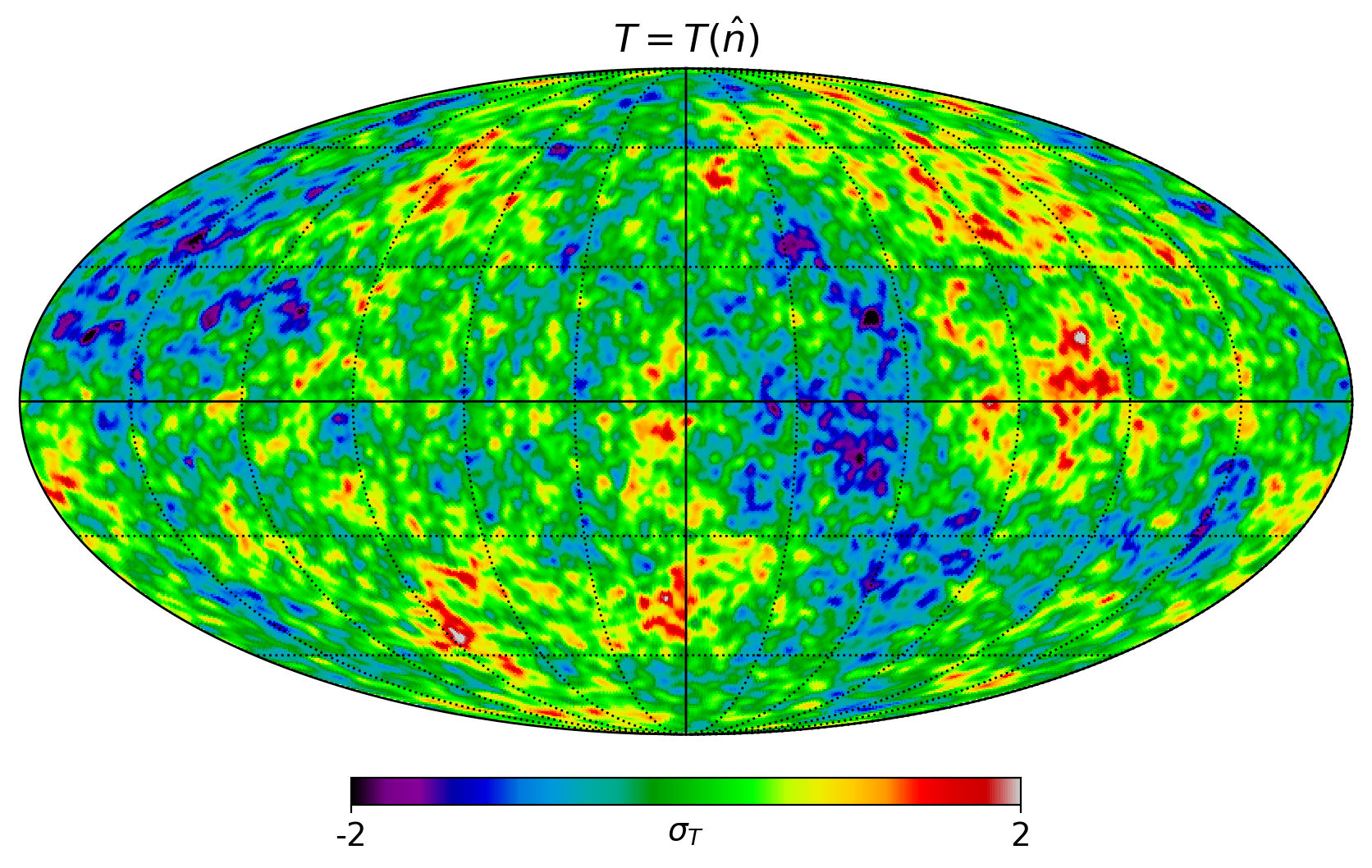
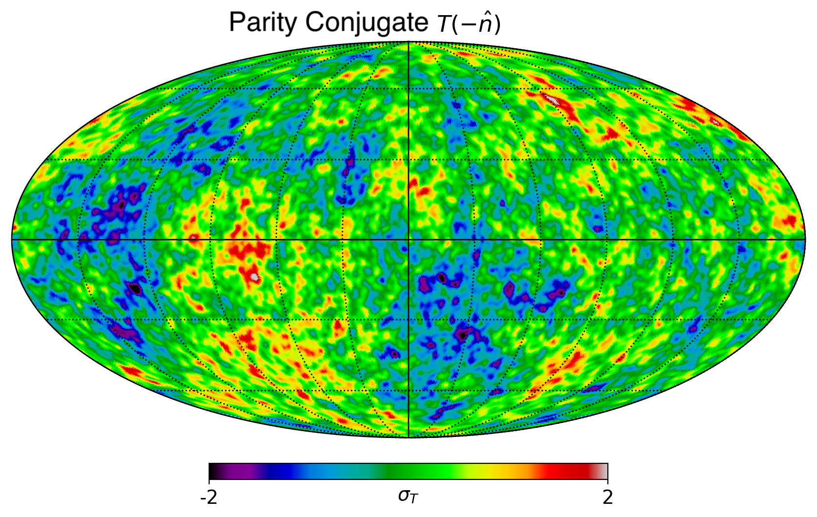
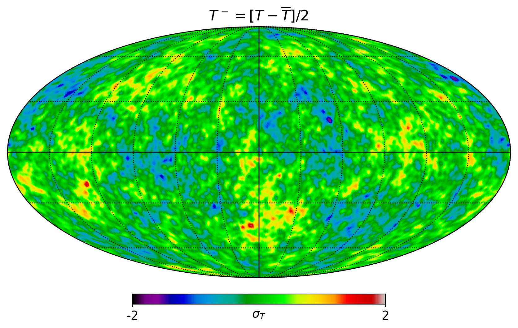
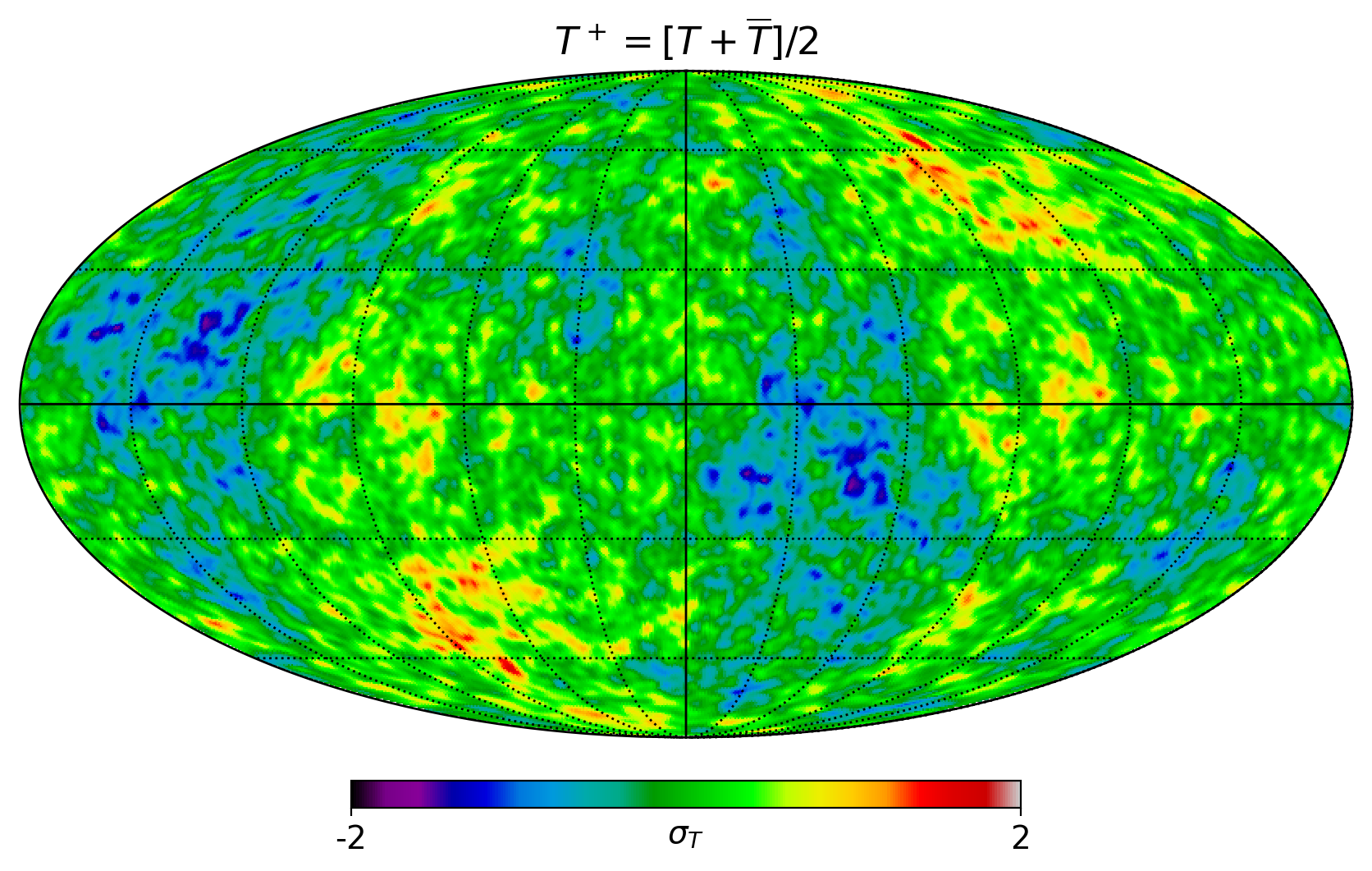
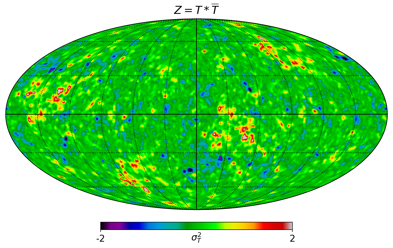
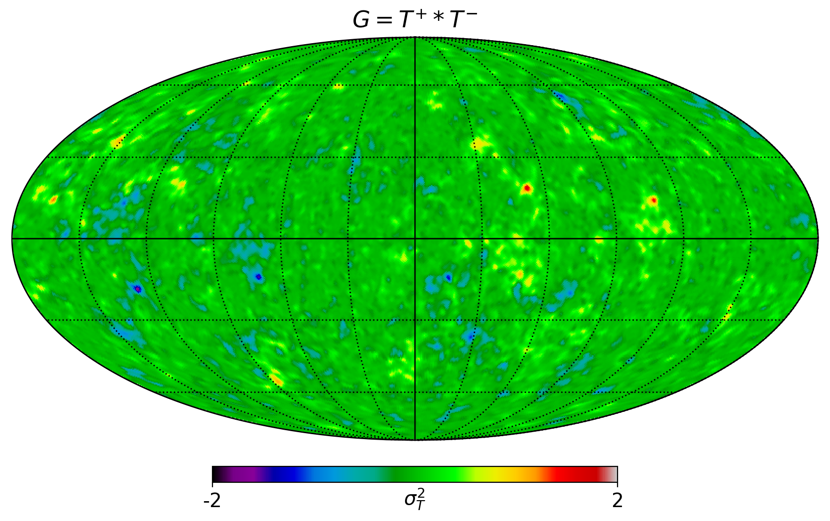
Figure 20: Same as Fig. 18 for a randomly selected realization of the SI+LCDM (with standard primordial inflation, SI). On average LCDM shows more even distribution of power in the odd/even parity maps than the Planck map.

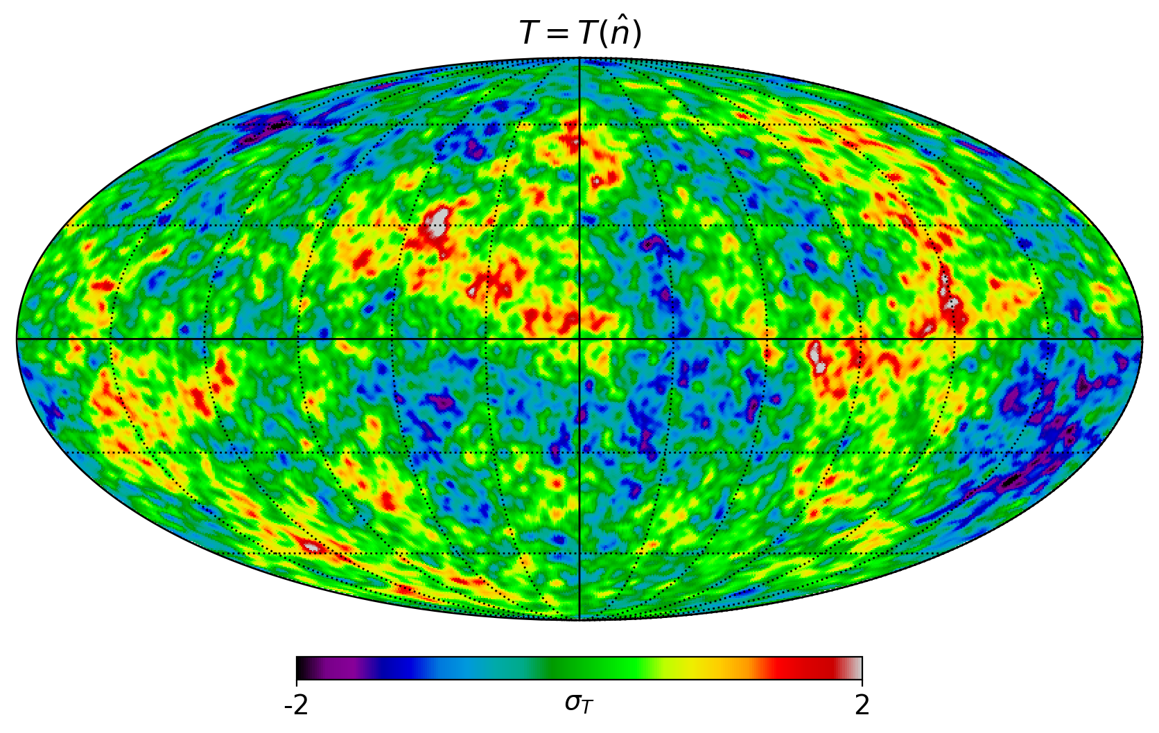
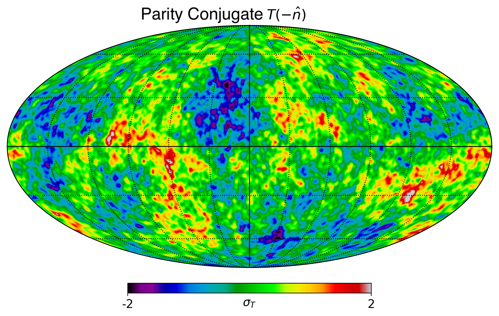
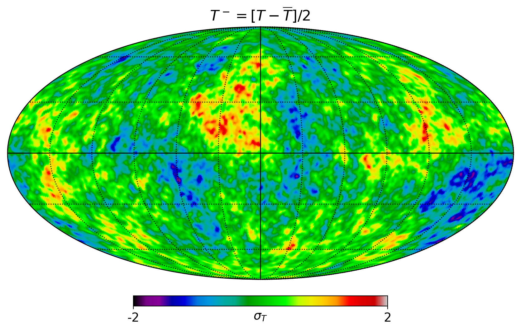
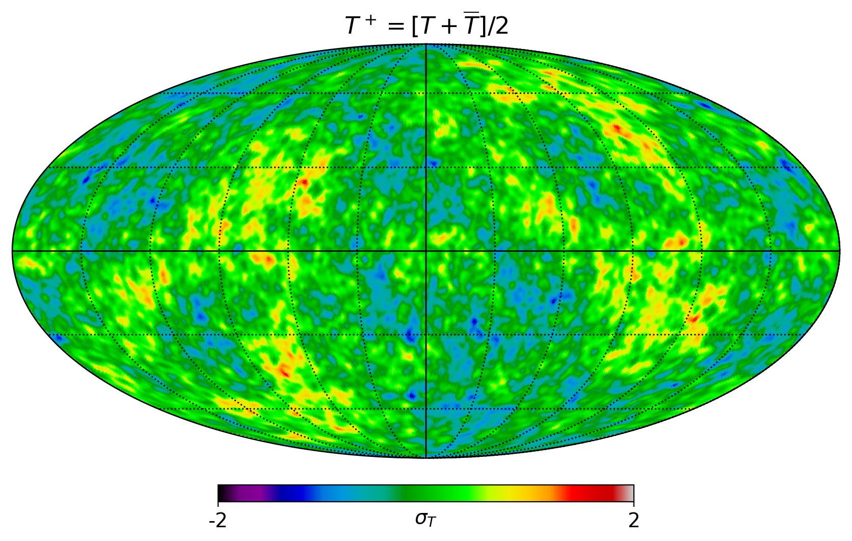
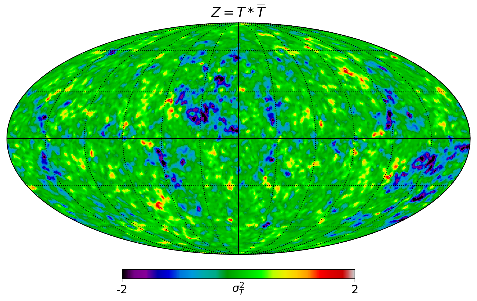
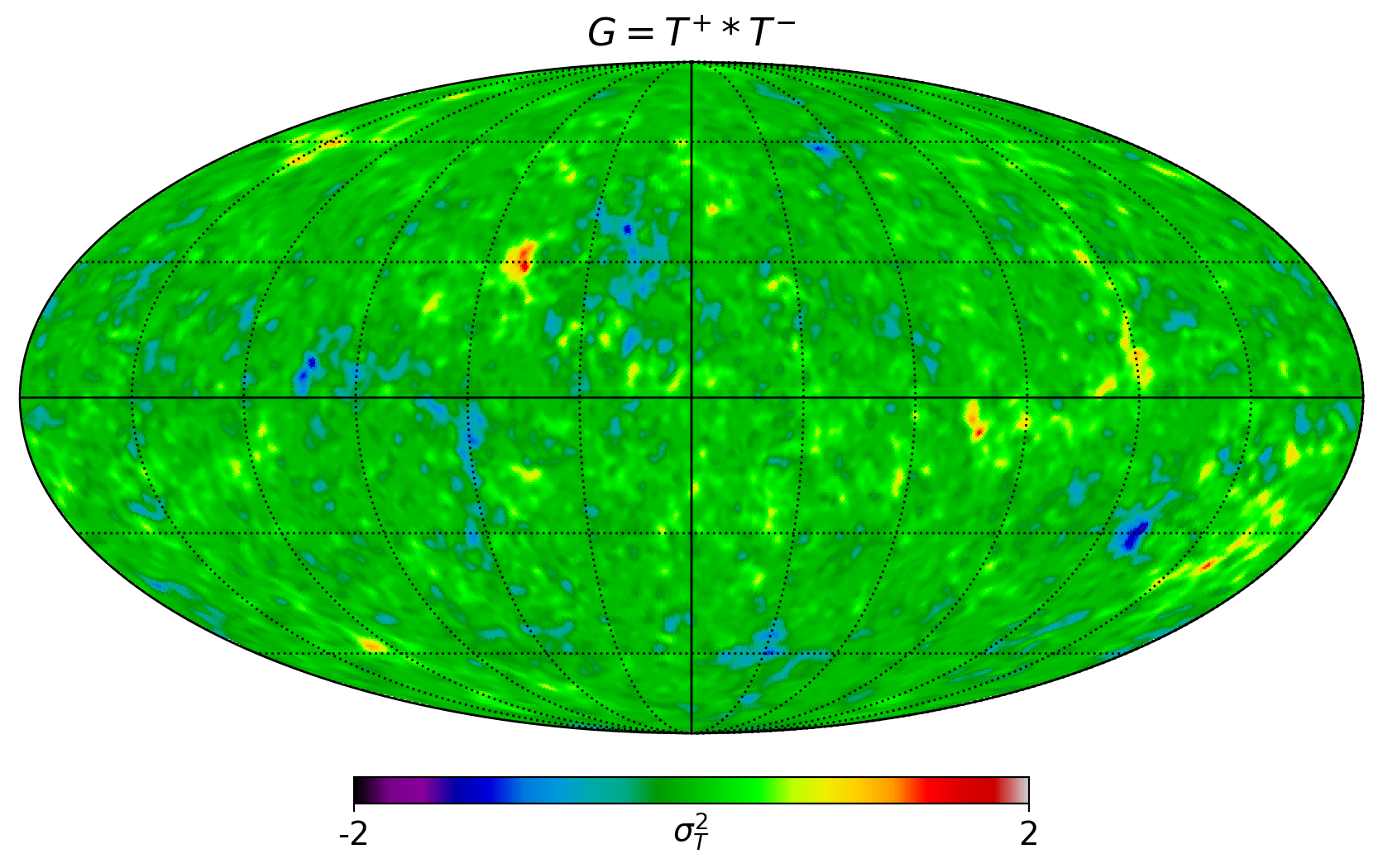
Figure 21: Same as Fig. 18 for a randomly selected realization of the DSI+LCDM. It shows prominent odd parity maps $T^{-}$ and negative values of $Z$, as in the observed Planck map.

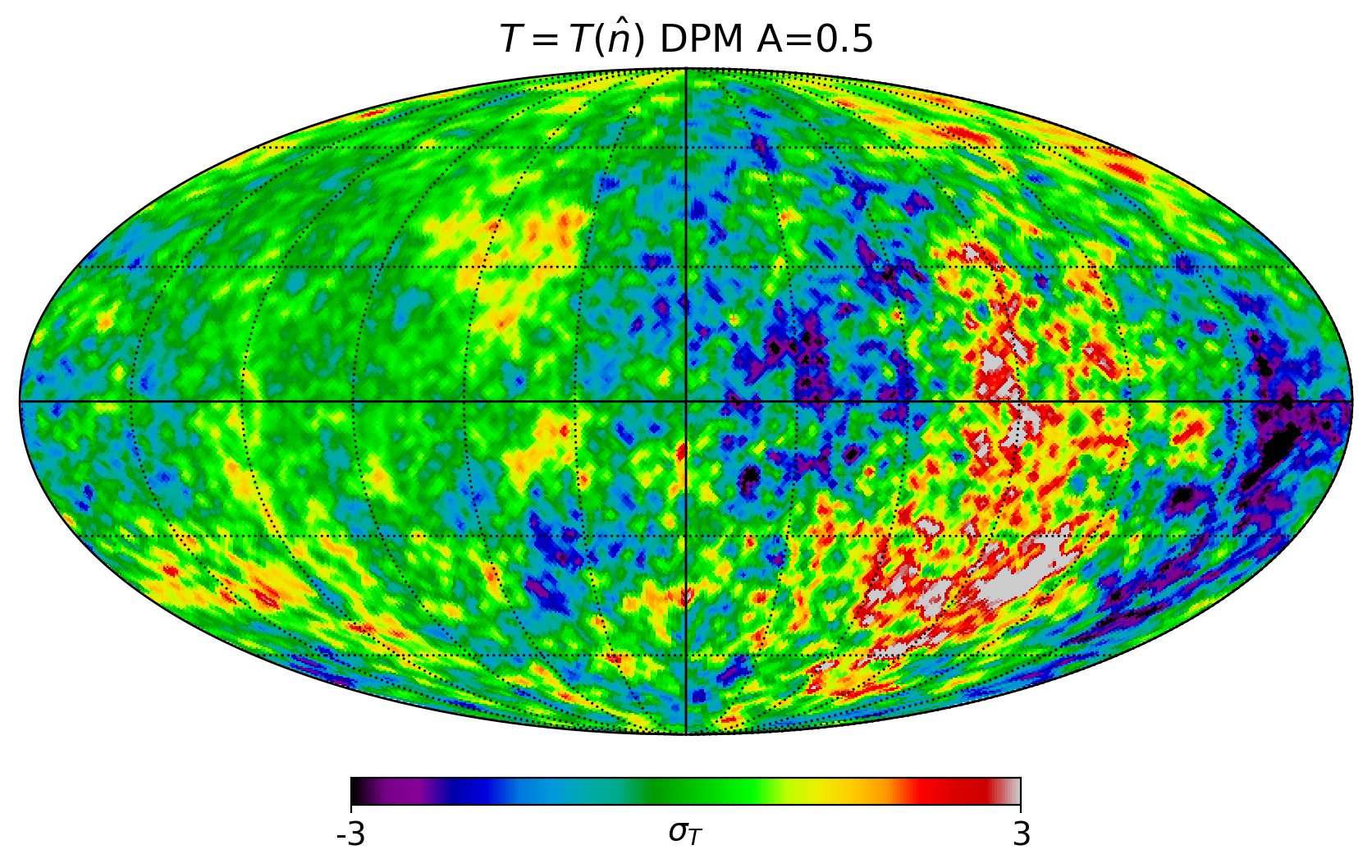
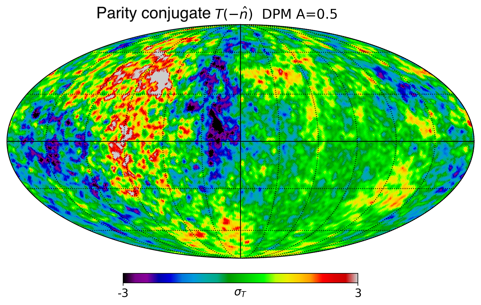
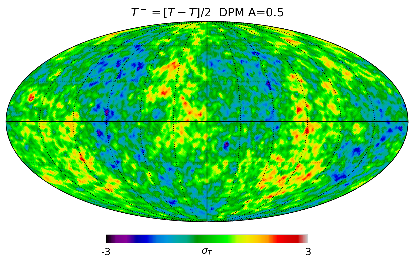
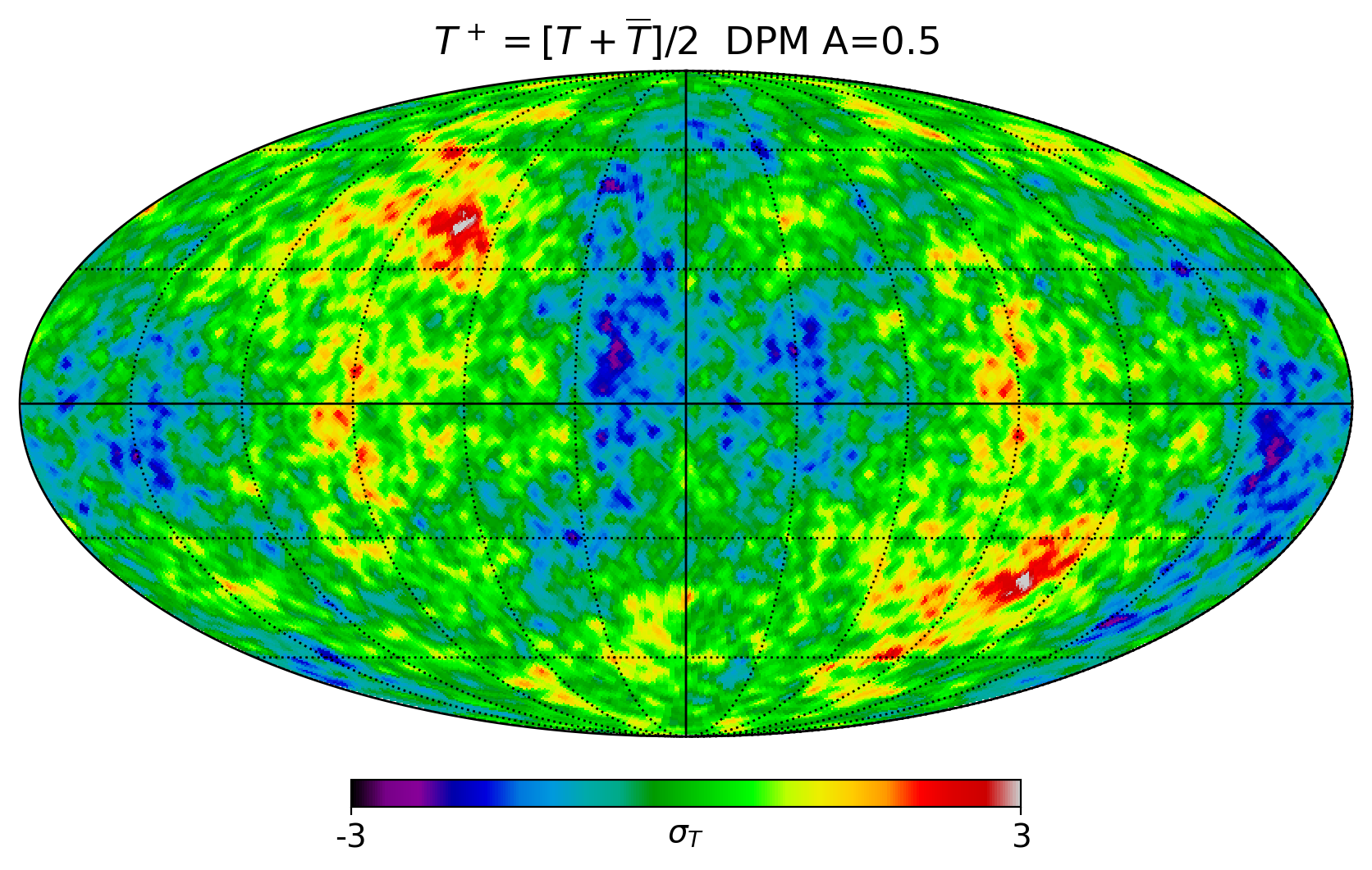
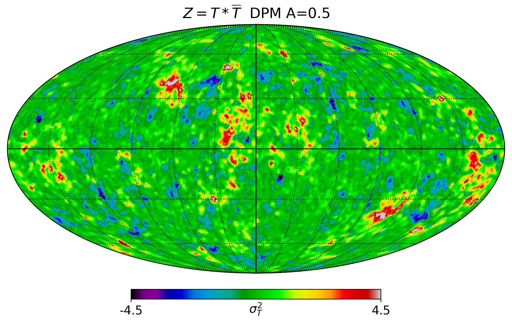
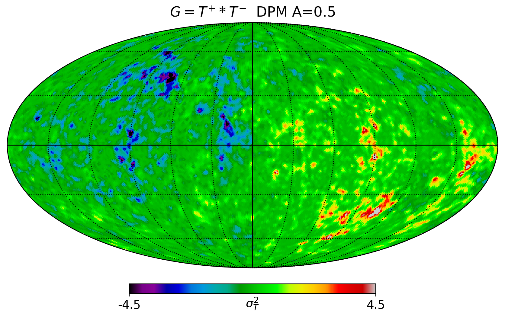
Figure 22: Same as Fig. 18 for a randomly selected realization of the extremely anisotropic DPM model with $A=0.5$. Despite the very large dipolar anisotropy, the model shows no preference for odd parity in the $Z$ maps other than some rare peaks at the position of North and South Ecliptic poles, where the dipole mimics parity. Such rare peaks have little impact on the overall parity statistics (especially when we include a 4-$\sigma$ clipping).

References

- (1) T. D. Lee and C.-N. Yang, “Question of Parity Conservation in Weak Interactions,” Phys. Rev. 104 (1956) 254–258.
- (2) C. S. Wu, E. Ambler, R. W. Hayward, D. D. Hoppes, and R. P. Hudson, “Experimental Test of Parity Conservation in Decay,” Phys. Rev. 105 (1957) 1413–1414.
- (3) J. H. Christenson, J. W. Cronin, V. L. Fitch, and R. Turlay, “Evidence for the Decay of the Meson,” Phys. Rev. Lett. 13 (1964) 138–140.
- (4) S. Coleman, Lectures of Sidney Coleman on Quantum Field Theory. WSP, Hackensack, 12, 2018.
- (5) A. D. Sakharov, “Violation of CP Invariance, C asymmetry, and baryon asymmetry of the universe,” Pisma Zh. Eksp. Teor. Fiz. 5 (1967) 32–35.
- (6) L. Canetti, M. Drewes, and M. Shaposhnikov, “Matter and Antimatter in the Universe,” New J. Phys. 14 (2012) 095012, arXiv:1204.4186 [hep-ph].
- (7) J. P. Kaufman, B. G. Keating, and B. R. Johnson, “Precision Tests of Parity Violation over Cosmological Distances,” Mon. Not. Roy. Astron. Soc. 455 no. 2, (2016) 1981–1988, arXiv:1409.8242 [astro-ph.CO].
- (8) K. Land and J. Magueijo, “The Axis of evil,” Phys. Rev. Lett. 95 (2005) 071301, arXiv:astro-ph/0502237.
- (9) J. Hoftuft, H. Eriksen, A. Banday, K. Gorski, F. Hansen, and P. Lilje, “Increasing evidence for hemispherical power asymmetry in the five-year WMAP data,” Astrophys. J. 699 (2009) 985–989, arXiv:0903.1229 [astro-ph.CO].
- (10) S. Mukherjee, P. K. Aluri, S. Das, S. Shaikh, and T. Souradeep, “Direction dependence of cosmological parameters due to cosmic hemispherical asymmetry,” JCAP 06 (2016) 042, arXiv:1510.00154 [astro-ph.CO].
- (11) Y. Akrami, Y. Fantaye, A. Shafieloo, H. K. Eriksen, F. K. Hansen, A. J. Banday, and K. M. Górski, “Power asymmetry in WMAP and Planck temperature sky maps as measured by a local variance estimator,” Astrophys. J. Lett. 784 (2014) L42, arXiv:1402.0870 [astro-ph.CO].
- (12) J. Jones, C. J. Copi, G. D. Starkman, and Y. Akrami, “The Universe is not statistically isotropic,” arXiv:2310.12859 [astro-ph.CO].
- (13) G. Hinshaw, A. J. Branday, C. L. Bennett, K. M. Gorski, A. Kogut, C. H. Lineweaver, G. F. Smoot, and E. L. Wright, “Two-Point Correlations in the COBE DMR Four-Year Anisotropy Maps,” ApJl 464 (June, 1996) L25, arXiv:astro-ph/9601061 [astro-ph].
- (14) J. Lesgourgues, “Inflationary cosmology,” EPFL Lectures-Ecole Doctorale de Suisse Romande (2006) .
- (15) D. J. Schwarz, C. J. Copi, D. Huterer, and G. D. Starkman, “CMB Anomalies after Planck,” Class. Quant. Grav. 33 no. 18, (2016) 184001, arXiv:1510.07929 [astro-ph.CO].
- (16) R. Durrer, The Cosmic Microwave Background. Cambridge University Press, Cambridge, 2008.
- (17) Planck Collaboration, Y. Akrami et al., “Planck 2018 results. VII. Isotropy and Statistics of the CMB,” Astron. Astrophys. 641 (2020) A7, arXiv:1906.02552 [astro-ph.CO].
- (18) J. Muir, S. Adhikari, and D. Huterer, “Covariance of CMB anomalies,” Phys. Rev. D 98 no. 2, (2018) 023521, arXiv:1806.02354 [astro-ph.CO].
- (19) A. Lue, L.-M. Wang, and M. Kamionkowski, “Cosmological signature of new parity violating interactions,” Phys. Rev. Lett. 83 (1999) 1506–1509, arXiv:astro-ph/9812088.
- (20) N. Bartolo and G. Orlando, “Parity breaking signatures from a Chern-Simons coupling during inflation: the case of non-Gaussian gravitational waves,” JCAP 07 (2017) 034, arXiv:1706.04627 [astro-ph.CO].
- (21) Y. Minami and E. Komatsu, “New Extraction of the Cosmic Birefringence from the Planck 2018 Polarization Data,” Phys. Rev. Lett. 125 no. 22, (2020) 221301, arXiv:2011.11254 [astro-ph.CO].
- (22) O. H. E. Philcox, “Do the CMB Temperature Fluctuations Conserve Parity?,” Phys. Rev. Lett. 131 no. 18, (2023) 181001, arXiv:2303.12106 [astro-ph.CO].
- (23) J. Creswell and P. Naselsky, “Asymmetry of the CMB map: local and global anomalies,” JCAP 03 (2021) 103, arXiv:2102.13442 [astro-ph.CO].
- (24) A. A. Starobinsky, “A New Type of Isotropic Cosmological Models Without Singularity,” Phys. Lett. B91 (1980) 99–102.
- (25) A. H. Guth, “The Inflationary Universe: A Possible Solution to the Horizon and Flatness Problems,” Phys. Rev. D23 (1981) 347–356.
- (26) A. D. Linde, “A New Inflationary Universe Scenario: A Possible Solution of the Horizon, Flatness, Homogeneity, Isotropy and Primordial Monopole Problems,” Phys. Lett. 108B (1982) 389–393. [Adv. Ser. Astrophys. Cosmol.3,149(1987)].
- (27) Planck Collaboration, Y. Akrami et al., “Planck 2018 results. X. Constraints on inflation,” Astron. Astrophys. 641 (2020) A10, arXiv:1807.06211 [astro-ph.CO].
- (28) R. Durrer, The Cosmic Microwave Background. Cambridge University Press, 12, 2020.
- (29) V. F. Mukhanov and G. V. Chibisov, “Quantum Fluctuations and a Nonsingular Universe,” JETP Lett. 33 (1981) 532–535. [Pisma Zh. Eksp. Teor. Fiz.33,549(1981)].
- (30) F. K. Hansen, A. J. Banday, K. M. Gorski, H. K. Eriksen, and P. B. Lilje, “Power Asymmetry in Cosmic Microwave Background Fluctuations from Full Sky to Sub-degree Scales: Is the Universe Isotropic?,” Astrophys. J. 704 (2009) 1448–1458, arXiv:0812.3795 [astro-ph].
- (31) R. Sinha and T. Souradeep, “Post-wmap assessment of infrared cutoff in the primordial spectrum from inflation,” Phys. Rev. D 74 (2006) 043518, arXiv:astro-ph/0511808.
- (32) C. R. Contaldi, M. Peloso, L. Kofman, and A. D. Linde, “Suppressing the lower multipoles in the CMB anisotropies,” JCAP 07 (2003) 002, arXiv:astro-ph/0303636.
- (33) A. Iqbal, J. Prasad, T. Souradeep, and M. A. Malik, “Joint Planck and WMAP Assessment of Low CMB Multipoles,” JCAP 06 (2015) 014, arXiv:1501.02647 [astro-ph.CO].
- (34) F. G. Pedro and A. Westphal, “Low- CMB power loss in string inflation,” JHEP 04 (2014) 034, arXiv:1309.3413 [hep-th].
- (35) I. Agullo, D. Kranas, and V. Sreenath, “Large scale anomalies in the CMB and non-Gaussianity in bouncing cosmologies,” Class. Quant. Grav. 38 no. 6, (2021) 065010, arXiv:2006.09605 [astro-ph.CO].
- (36) V. F. Mukhanov, H. A. Feldman, and R. H. Brandenberger, “Theory of cosmological perturbations. Part 1. Classical perturbations. Part 2. Quantum theory of perturbations. Part 3. Extensions,” Phys. Rept. 215 (1992) 203–333.
- (37) K. S. Kumar and J. Marto, “Hemispherical asymmetry of primordial power spectra,” arXiv:2209.03928 [gr-qc].
- (38) K. S. Kumar and J. Marto, “Towards a unitary formulation of quantum field theory in curved spacetime I: the case of de Sitter spacetime,” arXiv:2305.06046 [hep-th].
- (39) K. S. Kumar and J. a. Marto, “Towards a unitary formulation of quantum field theory in curved space-time II: the case of Schwarzschild black hole,” arXiv:2307.10345 [hep-th].
- (40) B. Camacho-Quevedo and E. Gaztañaga, “A measurement of the scale of homogeneity in the early Universe,” JCAP 04 no. 04, (2022) 044, arXiv:2106.14303 [astro-ph.CO].
- (41) E. Gaztañaga, J. Wagg, T. Multamäki, A. Montaña, and D. H. Hughes, “Two-point anisotropies in WMAP and the cosmic quadrupole,” MNRAS 346 no. 1, (Nov., 2003) 47–57, arXiv:astro-ph/0304178 [astro-ph].
- (42) M. H. Namjoo, A. A. Abolhasani, S. Baghram, and H. Firouzjahi, “CMB Hemispherical Asymmetry: Long Mode Modulation and non-Gaussianity,” JCAP 08 (2014) 002, arXiv:1405.7317 [astro-ph.CO].
- (43) A. L. Erickcek, S. M. Carroll, and M. Kamionkowski, “Superhorizon Perturbations and the Cosmic Microwave Background,” Phys. Rev. D 78 (2008) 083012, arXiv:0808.1570 [astro-ph].
- (44) A. L. Erickcek, M. Kamionkowski, and S. M. Carroll, “A Hemispherical Power Asymmetry from Inflation,” Phys. Rev. D 78 (2008) 123520, arXiv:0806.0377 [astro-ph].
- (45) N. J. Secrest, S. von Hausegger, M. Rameez, R. Mohayaee, S. Sarkar, and J. Colin, “A Test of the Cosmological Principle with Quasars,” Astrophys. J. Lett. 908 no. 2, (2021) L51, arXiv:2009.14826 [astro-ph.CO].
- (46) P. K. Aluri et al., “Is the Observable Universe Consistent with the Cosmological Principle?,” arXiv:2207.05765 [astro-ph.CO].
- (47) M. Quartin and A. Notari, “On the significance of power asymmetries in Planck CMB data at all scales,” JCAP 01 (2015) 008, arXiv:1408.5792 [astro-ph.CO].
- (48) E. Gaztañaga, “The cosmological constant as a zero action boundary,” MNRAS 502 no. 1, (Mar., 2021) 436–444, arXiv:2101.07368 [gr-qc].
- (49) E. Gaztanaga, “How the Big Bang Ends Up Inside a Black Hole,” Universe 8 no. 5, (Apr., 2022) 257, arXiv:2204.11608 [astro-ph.CO].
- (50) E. Gaztañaga, “The Black Hole Universe, Part I,” Symmetry 14 no. 9, (Sept., 2022) 1849.
- (51) E. Gaztañaga, “The Black Hole Universe, Part II,” Symmetry 14 no. 10, (Sept., 2022) 1984.
- (52) E. Gaztanaga, “Do White Holes Exist?,” Universe 9 no. 4, (Apr., 2023) 194.
- (53) P. Fosalba and E. Gaztañaga, “Explaining cosmological anisotropy: evidence for causal horizons from CMB data,” MNRAS 504 no. 4, (July, 2021) 5840–5862.
- (54) E. Gaztanaga and B. Camacho-Quevedo, “What moves the heavens above?,” Phys. Lett. B 835 (2022) 137468, arXiv:2204.10728 [astro-ph.CO].
- (55) E. Gaztañaga, “The mass of our observable Universe,” MNRAS 521 no. 1, (May, 2023) L59–L63.
- (56) A. A. Starobinsky, “Nonsingular Model of the Universe with the Quantum Gravitational De Sitter Stage and its Observational Consequences,” in *Moscow 1981, Proceedings of the second seminar “Quantum Theory of Gravity”*, 58-72. 1981.
- (57) A. S. Koshelev, K. Sravan Kumar, and A. A. Starobinsky, “ inflation to probe non-perturbative quantum gravity,” JHEP 03 (2018) 071, arXiv:1711.08864 [hep-th].
- (58) A. S. Koshelev, K. S. Kumar, and A. A. Starobinsky, “Generalized non-local R2-like inflation,” JHEP 07 (2023) 146, arXiv:2209.02515 [hep-th].
- (59) A. S. Koshelev, K. S. Kumar, and A. A. Starobinsky, “Cosmology in nonlocal gravity,” arXiv:2305.18716 [hep-th].
- (60) A. Linde, “Inflationary Cosmology after Planck 2013,” in 100e Ecole d’Ete de Physique: Post-Planck Cosmology, pp. 231–316. 2015. arXiv:1402.0526 [hep-th].
- (61) J. Ellis, D. V. Nanopoulos, and K. A. Olive, “Starobinsky-like Inflationary Models as Avatars of No-Scale Supergravity,” JCAP 1310 (2013) 009, arXiv:1307.3537 [hep-th].
- (62) W. H. Kinney, “TASI Lectures on Inflation,” arXiv:0902.1529 [astro-ph.CO].
- (63) B. A. Powell and W. H. Kinney, “The pre-inflationary vacuum in the cosmic microwave background,” Phys. Rev. D 76 (2007) 063512, arXiv:astro-ph/0612006.
- (64) V. Vennin, Cosmological Inflation: Theoretical Aspects and Observational Constraints. Theses, Université Pierre et Marie Curie, Sept., 2014. https://theses.hal.science/tel-01094199.
- (65) C. Kiefer, Quantum Gravity. Oxford University Press, New York, 2nd ed ed., 2007.
- (66) C. Rovelli, Quantum gravity. Cambridge Monographs on Mathematical Physics. Univ. Pr., Cambridge, UK, 2004.
- (67) V. Vennin and A. A. Starobinsky, “Correlation Functions in Stochastic Inflation,” Eur. Phys. J. C 75 (2015) 413, arXiv:1506.04732 [hep-th].
- (68) M. Spradlin, A. Strominger, and A. Volovich, “Les Houches lectures on de Sitter space,” in Les Houches Euro Summer School: on Unity of Fundamental Physics: Gravity, Gauge Theory and Strings, pp. 423–453. 10, 2001. arXiv:hep-th/0110007.
- (69) T. Hartman, Y. Jiang, and E. Shaghoulian, “Islands in cosmology,” JHEP 11 (2020) 111, arXiv:2008.01022 [hep-th].
- (70) Erwin Schrodinger, Expanding universes. 1956.
- (71) M. K. Parikh, I. Savonije, and E. P. Verlinde, “Elliptic de Sitter space: dS/Z(2),” Phys. Rev. D 67 (2003) 064005, arXiv:hep-th/0209120.
- (72) D. Polarski and A. A. Starobinsky, “Semiclassicality and decoherence of cosmological perturbations,” Class. Quant. Grav. 13 (1996) 377–392, arXiv:gr-qc/9504030.
- (73) C. Kiefer, D. Polarski, and A. A. Starobinsky, “Quantum to classical transition for fluctuations in the early universe,” Int. J. Mod. Phys. D 7 (1998) 455–462, arXiv:gr-qc/9802003.
- (74) D. Sudarsky, “Shortcomings in the Understanding of Why Cosmological Perturbations Look Classical,” Int. J. Mod. Phys. D 20 (2011) 509–552, arXiv:0906.0315 [gr-qc].
- (75) S. Landau, G. León, and D. Sudarsky, “Quantum Origin of the Primordial Fluctuation Spectrum and its Statistics,” Phys. Rev. D 88 no. 2, (2013) 023526, arXiv:1107.3054 [astro-ph.CO].
- (76) D. Cruces, “Review on Stochastic Approach to Inflation,” Universe 8 no. 6, (2022) 334, arXiv:2203.13852 [gr-qc].
- (77) A. A. Starobinsky, “The Perturbation Spectrum Evolving from a Nonsingular Initially De-Sitter Cosmology and the Microwave Background Anisotropy,” Sov. Astron. Lett. 9 (1983) 302–304.
- (78) R. Mahbub and A. De, “Smooth coarse-graining and colored noise dynamics in stochastic inflation,” JCAP 09 (2022) 045, arXiv:2204.03859 [astro-ph.CO].
- (79) C. Pattison, V. Vennin, H. Assadullahi, and D. Wands, “Quantum diffusion during inflation and primordial black holes,” JCAP 10 (2017) 046, arXiv:1707.00537 [hep-th].
- (80) C. Pattison, V. Vennin, H. Assadullahi, and D. Wands, “Stochastic inflation beyond slow roll,” JCAP 07 (2019) 031, arXiv:1905.06300 [astro-ph.CO].
- (81) F. Finelli, G. Marozzi, G. P. Vacca, and G. Venturi, “Energy momentum tensor of field fluctuations in massive chaotic inflation,” Phys. Rev. D 65 (2002) 103521, arXiv:gr-qc/0111035.
- (82) N. C. Tsamis and R. P. Woodard, “Stochastic quantum gravitational inflation,” Nucl. Phys. B 724 (2005) 295–328, arXiv:gr-qc/0505115.
- (83) F. Finelli, G. Marozzi, A. A. Starobinsky, G. P. Vacca, and G. Venturi, “Stochastic growth of quantum fluctuations during inflation,” AIP Conf. Proc. 1446 no. 1, (2012) 320–332, arXiv:1102.0216 [hep-th].
- (84) F. Finelli, G. Marozzi, A. A. Starobinsky, G. P. Vacca, and G. Venturi, “Generation of fluctuations during inflation: Comparison of stochastic and field-theoretic approaches,” Phys. Rev. D 79 (2009) 044007, arXiv:0808.1786 [hep-th].
- (85) A. A. Starobinsky, “STOCHASTIC DE SITTER (INFLATIONARY) STAGE IN THE EARLY UNIVERSE,” Lect. Notes Phys. 246 (1986) 107–126.
- (86) A. A. Starobinsky and J. Yokoyama, “Equilibrium state of a selfinteracting scalar field in the De Sitter background,” Phys. Rev. D 50 (1994) 6357–6368, arXiv:astro-ph/9407016.
- (87) T. Fujita, M. Kawasaki, and Y. Tada, “Non-perturbative approach for curvature perturbations in stochastic formalism,” JCAP 10 (2014) 030, arXiv:1405.2187 [astro-ph.CO].
- (88) S. S. Mishra, E. J. Copeland, and A. M. Green, “Primordial black holes and stochastic inflation beyond slow roll. Part I. Noise matrix elements,” JCAP 09 (2023) 005, arXiv:2303.17375 [astro-ph.CO].
- (89) J. H. P. Jackson, H. Assadullahi, K. Koyama, V. Vennin, and D. Wands, “Numerical simulations of stochastic inflation using importance sampling,” JCAP 10 (2022) 067, arXiv:2206.11234 [astro-ph.CO].
- (90) CMB-S4 Collaboration, K. N. Abazajian et al., “CMB-S4 Science Book, First Edition,” arXiv:1610.02743 [astro-ph.CO].
- (91) A. G. Riess, S. Casertano, W. Yuan, J. B. Bowers, L. Macri, J. C. Zinn, and D. Scolnic, “Cosmic Distances Calibrated to 1% Precision with Gaia EDR3 Parallaxes and Hubble Space Telescope Photometry of 75 Milky Way Cepheids Confirm Tension with CDM,” ApJL 908 no. 1, (Feb., 2021) L6, arXiv:2012.08534 [astro-ph.CO].
- (92) E. Di Valentino, O. Mena, S. Pan, L. Visinelli, W. Yang, A. Melchiorri, D. F. Mota, A. G. Riess, and J. Silk, “In the realm of the Hubble tension—a review of solutions,” Class. Quant. Grav. 38 no. 15, (2021) 153001, arXiv:2103.01183 [astro-ph.CO].
- (93) J. R. Bond, A. H. Jaffe, and L. Knox, “Radical Compression of Cosmic Microwave Background Data,” ApJ 533 no. 1, (Apr., 2000) 19–37, arXiv:astro-ph/9808264 [astro-ph].
- (94) K. Land and J. Magueijo, “Is the Universe odd?,” PRD 72 no. 10, (Nov., 2005) 101302, arXiv:astro-ph/0507289 [astro-ph].
- (95) J.-S. Kim, P. Naselskya, and M. Hansen, “Symmetry and anti-symmetry of the CMB anisotropy pattern,” Adv. Astron. 2012 (2012) 960509, arXiv:1202.0728 [astro-ph.CO].
- (96) D. N. Spergel, L. Verde, H. V. Peiris, E. Komatsu, M. R. Nolta, C. L. Bennett, M. Halpern, G. Hinshaw, N. Jarosik, A. Kogut, M. Limon, S. S. Meyer, L. Page, G. S. Tucker, J. L. Weiland, E. Wollack, and E. L. Wright, “First-Year Wilkinson Microwave Anisotropy Probe (WMAP) Observations: Determination of Cosmological Parameters,” ApJs 148 no. 1, (Sept., 2003) 175–194, arXiv:astro-ph/0302209 [astro-ph].
- (97) Planck Collaboration, P. A. R. Ade et al., “Planck 2013 results. XXIII. Isotropy and statistics of the CMB,” Astron. Astrophys. 571 (2014) A23, arXiv:1303.5083 [astro-ph.CO].
- (98) B. B. Mandelbrot, The Fractal Geometry of Nature. 1982.
- (99) B. B. Mandelbrot, “Galaxy distributions and fractals.,” Astrophysical Letters and Communications 36 (Dec., 1997) 1–5.