Simultaneous Change Point Detection and Identification for High Dimensional Linear Models

Abstract

In this article, we consider change point inference for high dimensional linear models. For change point detection, given any subgroup of variables, we propose a new method for testing the homogeneity of corresponding regression coefficients across the observations. Under some regularity conditions, the proposed new testing procedure controls the type I error asymptotically and is powerful against sparse alternatives and enjoys certain optimality. For change point identification, an “argmax” based change point estimator is proposed which is shown to be consistent for the true change point location. Moreover, combining with the binary segmentation technique, we further extend our new method for detecting and identifying multiple change points. Extensive numerical studies justify the validity of our new method and an application to the Alzheimer’s disease data analysis further demonstrate its competitive performance.

Keyword: Change point inference, High dimensions, Linear regression, Multiplier bootstrap, Sparsity, Subgroups.

1 Introduction

Driven by the great improvement of data collection and storage capacity, high dimensional linear regression models have attracted a lot of attentions because of its simplicity for interpreting the effect of different variables in predicting the response. Specifically, we are interested in the following model:

$$Y=\bm{X}^{\top}\bm{\beta}+\epsilon,$$

where $Y\in\mathbb{R}$ is the response variable, $\bm{X}=(X_{1},\ldots,X_{p})\in\mathbb{R}^{p}$ is the covariate vector, $\bm{\beta}=(\beta_{1},\ldots,\beta_{p})^{\top}$ is a $p$-dimensional unknown vector of coefficients, and $\epsilon\in\mathbb{R}$ is the error term.

For high dimensional linear regression, the $L_{1}$-penalized technique lasso (Tibshirani (1996)) is a popular method for estimating $\bm{\beta}$. In the past decades, lots of research attentions both in machine learning and statistics have been focused on studying theoretical properties of lasso and other penalized methods. Most of the existing literature on high dimensional linear regression focuses on the case with a homogeneous linear model, where the regression coefficients are assumed invariant across the observations. With many modern complex datasets for analysis in practice, data heterogeneity is a common challenge in many real applications such as economy and genetics. In some applications, the regression coefficients may have a sudden change at some unknown time point, which is called a change point. Typical examples include racial segregation and crime prediction in sociology, and financial contagion in economy. For these problems, methods and theories designed for independently and identically ($i.i.d.$) distributed settings are no longer applicable. As a result, ignoring these structural breaks in machine learning applications may lead to misleading results and wrong decision making. For the regression change point problem, a fundamental question is whether the underlying regression model remains homogenous across the observations. To address this issue, in this article, we investigate change point inference for high dimensional linear models. Specifically, let $(Y_{i},\bm{X}_{i})_{i=1}^{n}$ be $n$ ordered independent realizations of $(Y,\bm{X})$. We aim to detect whether the regression coefficients have a change point during the observations. In particular, let $\bm{\beta}^{(1)}$ and $\bm{\beta}^{(2)}$ be two $p$-dimensional vectors of coefficients with $\bm{\beta}^{(1)}=(\beta^{(1)}_{1},\ldots,\beta^{(1)}_{p})^{\top}$ and $\bm{\beta}^{(2)}=(\beta^{(2)}_{1},\ldots,\beta^{(2)}_{p})^{\top}$. We consider the following linear regression model with a possible change point:

$$\begin{array}[]{ll}Y_{i}=\bm{X}_{i}^{\top}\bm{\beta}^{(1)}\mathbf{1}\{1\leq i\leq k_{*}\}+\bm{X}_{i}^{\top}\bm{\beta}^{(2)}\mathbf{1}\{k_{*}+1\leq i\leq n\}+\epsilon_{i},\end{array}$$ (1.1)

where $k_{*}$ is the possible but unknown change point location and $(\epsilon_{i})_{i=1}^{n}$ are the error terms. In this paper, we assume $k_{*}=\lfloor nt_{0}\rfloor$ for some $t_{0}\in(0,1)$. For any given subgroup $\mathcal{G}\subset\{1,\ldots,p\}$, the first goal is to test

$$\begin{array}[]{ll}\mathbf{H}_{0,\mathcal{G}}:\beta_{s}^{(1)}=\beta_{s}^{(2)}~{}~{}\text{for~{}all}~{}s\in\mathcal{G}~{}~{}\text{v.s.}{}{}\\ \mathbf{H}_{1,\mathcal{G}}:\text{There exist}~{}s\in\mathcal{G}~{}\text{and}~{}k_{*}\in\{1,\dots,n-1\}~{}\text{s.t.}~{}\beta_{s}^{(1)}\neq\beta_{s}^{(2)}.\end{array}$$ (1.2)

In other words, under $\mathbf{H}_{0,\mathcal{G}}$, the regression coefficients in each subgroup $\mathcal{G}$ are homogeneous across the observations, and under $\mathbf{H}_{1,\mathcal{G}}$ there is a change point at an unknown time point $k_{*}$ such that the regression coefficients have a sudden change after $k_{*}$. Our second goal of the paper is to identify the change point location once we reject $\mathbf{H}_{0,\mathcal{G}}$ in (1.2). In this paper, we assume that the number of coefficients can be much larger than the number of observations, i.e., $p\succeq n$, which is known as a high dimensional problem.

For the low dimensional setting with a fixed $p$ and $p<n$, change point inference for linear regression models has been well-studied. For example, Quandt (1960) considered testing (1.2) for a simple regression model with $p=2$. Based on that, several techniques were proposed in the literature. Among them are maximum likelihood ratio tests (Horváth, 1995), partial sums of regression residuals (Bai and Perron, 1998), and the union intersection test (Horváth and Shao, 1995). Moreover, as a special case of linear regression models, Chan et al. (2014) considered change point detection for the autoregressive model. As compared to the broad literature in the low dimensional setting, methods and theory for high dimensional change point inference of (1.1) have not been investigated much until recently. For instance, Lee et al. (2016) considered a high dimensional regression model with a possible change point due to a covariate threshold. Based on the $L_{1}/L_{0}$ regularization, Kaul et al. (2019) proposed a two-step algorithm for the detection and estimation of parameters in a high-dimensional change point regression model. As extensions to multiple structural breaks in high dimensional linear models, Leonardi and Bühlmann (2016) proposed fast algorithms for multiple change point estimation based on dynamic programming and binary search algorithms. In addition, Zhang et al. (2015) developed an approach for estimating multiple change points based on sparse group lasso. Wang et al. (2021) proposed a projection-based algorithm for estimating multiple change points. Recently, Cho and Owens (2022); Bai and Safikhani (2023) constructed estimates for the multiple change points in high-dimensional regression models based on methods of moving window and blocked fused lasso. Kaul et al. (2021); Xu et al. (2022) respectively considered the problem of constructing confidence interval for the change point in the context of high dimensional mean vector-based models and linear regression models. Chen et al. (2023) proposed a new method for determing the number of change points with false discovery rate controls. Other related papers include He et al. (2023); Wang et al. (2022).

It is worth noting that the majority of above mentioned papers mainly focus on the estimation of regression coefficients as well as the change point locations by assuming a pre-existing change point in the model. To our best knowledge, the testing problem of (1.2) has not been considered yet. How to make effective change point detection remains to be an urgent but challenging task. To fill this gap, in this article, we consider change point inference in the context of high dimensional linear models.

The main contributions of this paper are as follows. For any pre-specified subgroup $\mathcal{G}\subset\{1,\ldots,p\}$, we propose a new method for testing the homogeneity of corresponding regression coefficients across the observations. For change point detection, the proposed test statistic $T_{\mathcal{G}}$ is constructed based on a weighted $L_{\infty}$ aggregation, both temporally and spatially, of the process $\{Z_{j}(\lfloor nt\rfloor)\}_{j\in\mathcal{G},t\in[\tau_{0},1-\tau_{0}]}$, where $Z_{j}(\lfloor nt\rfloor)=\breve{\beta}_{j}^{(0,t)}-\breve{\beta}_{j}^{(t,1)}$ with $\breve{\beta}_{j}^{(0,t)}$ and $\breve{\beta}_{j}^{(t,1)}$ denoting the de-biased lasso estimators for coordinate $j$ before and after time point $\lfloor nt\rfloor$, respectively. It is shown that $T_{\mathcal{G}}$ is powerful against sparse alternatives with only a few entries in $\mathcal{G}$ having a change point. To approximate its limiting null distribution, a multiplier bootstrap procedure is introduced. The proposed bootstrap can automatically account for the dependence structures of $\{Z_{j}(\lfloor nt\rfloor)\}_{j\in\mathcal{G},t\in[\tau_{0},1-\tau_{0}]}$ and allow the group size $|\mathcal{G}|$ to grow exponentially with the sample size $n$. Furthermore, to identify the change point location, for each time point $\lfloor nt\rfloor$, we first aggregate the coordinates with the $L_{\infty}$-norm, then a change point estimator $\widehat{t}_{0,\mathcal{G}}$ is obtained by taking “argmax” with respect to $t$ of the above aggregated process with some proper weights. In addition to single change point detection, by combining with the binary segmentation technique (Vostrikova, 1981), we extend our new algorithm for detecting multiple change points which enjoys better performance than the existing methods.

In terms of theoretical investigation, with mild moment conditions on the covariates and errors in the regression model, we justify the validity of our proposed method in terms of change point detection and identification. In particular, our bootstrap procedure consistently approximates the limiting null distribution of $T_{\mathcal{G}}$, which implies that the proposed new test preserves the pre-specified significance level asymptotically. Furthermore, under $\mathbf{H}_{1,\mathcal{G}}$, our new method is sensitive to sparse alternatives and can reject the null hypothesis with probability tending to one. It is worth mentioning that Xia et al. (2018) considered two sample tests for high dimensional linear regression models. They derived some conditions for consistently distinguishing two sample regression models, which are shown to be minimax optimal. Our requirement for detecting a change point under $\mathbf{H}_{1,\mathcal{G}}$ has the same order as the condition derived in Xia et al. (2018). As for the change point estimation, we prove that our proposed argmax-based change point estimator is consistent for $t_{0}$ with an estimation error rate of $\big{|}\widehat{t}_{0,\mathcal{G}}-t_{0}\big{|}=O_{p}\big{(}\dfrac{\log(|\mathcal{G}|n)}{n\|\bm{\delta}\|_{\mathcal{G},\infty}^{2}}\big{)},$ where $\bm{\delta}:=\bm{\beta}^{(1)}-\bm{\beta}^{(2)}$ with $\|\bm{\delta}\|_{\mathcal{G},\infty}=:\max_{j\in\mathcal{G}}|\beta_{j}^{(1)}-\beta_{j}^{(2)}|$. Hence, the above estimation result shows that our proposed change point estimator is consistent as long as $\|\bm{\beta}^{(1)}-\bm{\beta}^{(2)}\|_{\mathcal{G},\infty}\gg\sqrt{\log(|\mathcal{G}|n)/n}$ and allows the overall sparsity of regression coefficients and the group’s magnitude $|\mathcal{G}|$ to grow simultaneously with the sample size $n$. We demonstrate that our new testing procedure is relatively simple to implement and extensive numerical studies provide strong support to our theory. Moreover, an R package called “RegCpt” is developed to implement our proposed new algorithms.

The rest of this paper is organized as follows. In Section 2, we introduce our new methodology for Problem (1.2). In Section 3, some theoretical results are derived in terms of change point detection and identification. In Section 4, extensive numerical studies are investigated. The detailed proofs of the main theorems, additional numerical studies and an interesting real data application are given in the Appendix.

For $\bm{v}=(v_{1},\ldots,v_{p})^{\top}\in\mathbb{R}^{p}$, let its $L_{p}$ norm be $\|\bm{v}\|_{p}=(\sum_{j=1}^{d}|v_{j}|^{p})^{1/p}$ for $1\leq p\leq\infty$. For $p=\infty$, define $\|\bm{v}\|_{\infty}=\max_{1\leq j\leq d}|v_{j}|$. For a subset $\mathcal{G}\subset\{1,\ldots,p\}$, denote $\|\bm{v}\|_{\mathcal{G},\infty}$ by $\max_{j\in\mathcal{G}}|v_{j}|$. For any set ${\mathcal{S}}$, denote its cardinality by $|{\mathcal{S}}|$. For two real numbered sequences $a_{n}$ and $b_{n}$, set $a_{n}=O(b_{n})$ if there exits a constant $C$ such that $|a_{n}|\leq C|b_{n}|$ for a sufficiently large $n$; $a_{n}=o(b_{n})$ if $a_{n}/b_{n}\rightarrow 0$ as $n\rightarrow\infty$; $a_{n}\asymp b_{n}$ if there exists constants $c$ and $C$ such that $c|b_{n}|\leq|a_{n}|\leq C|b_{n}|$ for a sufficiently large $n$. For a sequence of random variables $\{\xi_{1},\xi_{2},\ldots\}$, denote $\xi_{n}=o_{p}(1)$ if $\xi_{n}\xrightarrow{{\mathbb{P}}}0$. Define $\lfloor x\rfloor$ as the largest integer less than or equal to $x$ for $x\geq 0$.

2 Methodology

2.1 New test statistic

We present our methodology for testing the existence of a change point in Model (1.1). To this end, we first introduce some basic model settings. Recall the regression model

$$Y_{i}=\bm{X}_{i}^{\top}\bm{\beta}^{(1)}\mathbf{1}\{1\leq i\leq\lfloor nt_{0}\rfloor\}+\bm{X}_{i}^{\top}\bm{\beta}^{(2)}\mathbf{1}\{\lfloor nt_{0}\rfloor+1\leq i\leq n\}+\epsilon_{i}.$$ (2.1)

Denote $\bm{Y}=(Y_{1},\ldots,Y_{n})^{\top}$ as a $n\times 1$ response vector, $\mathbf{X}$ is a $n\times p$ design matrix with $\bm{X}_{i}=(X_{i,1},\ldots,X_{i,p})^{\top}$ being its $i$-th row for $1\leq i\leq n$, and $\bm{\epsilon}=(\epsilon_{1},\cdots,\epsilon_{n})^{\top}$ is the error vector. For the unknown $p\times 1$ regression vectors $\bm{\beta}^{(1)}=(\beta_{1}^{(1)},\ldots,\beta_{p}^{(1)})^{\top}$ and $\bm{\beta}^{(2)}=(\beta_{1}^{(2)},\ldots,\beta_{p}^{(2)})^{\top}$, define ${\mathcal{S}}^{(1)}=\{1\leq j\leq p:\beta_{j}^{(1)}\neq 0\}$ and ${\mathcal{S}}^{(2)}=\{1\leq j\leq p:\beta_{j}^{(2)}\neq 0\}$ as the active sets of variables. Denote $s^{(1)}=|{\mathcal{S}}^{(1)}|$ and $s^{(2)}=|{\mathcal{S}}^{(2)}|$ as the cardinalities of ${\mathcal{S}}^{(1)}$ and ${\mathcal{S}}^{(2)}$, respectively. Define $\bm{\Sigma}=(\Sigma_{i,j})=\text{Cov}(\bm{X}_{1})$ as the covariance matrix of $\bm{X}_{1}$ and $\bm{\Theta}=(\theta_{i,j})$ as the inverse of $\bm{\Sigma}$. For $\bm{\Theta}$, let $s_{j}=|\{1\leq k\leq p:\theta_{j,k}\neq 0,k\neq j\}|$. In addition to the above notations, we assume that the change point does not happen at the beginning or end of data observations. In other words, there exists some $\tau_{0}\in(0,0.5)$ such that $t_{0}\in[\tau_{0},1-\tau_{0}]$ holds. Note that the search boundary scales with $n$ by allowing $\tau_{0}\rightarrow 0$.

To propose our method, we first introduce the de-sparsified (de-biased) lasso estimator, which was proposed in Van de Geer et al. (2014) and Zhang and Zhang (2014). Specifically, for Model (2.1), let $\widehat{\bm{\beta}}_{n}$ be a lasso estimator from $\widehat{\bm{\beta}}^{n}=\mathop{\text{\rm arg\,min}}_{\bm{\beta}\in\mathbb{R}^{p}}\|\bm{Y}-\mathbf{X}\bm{\beta}\|_{2}^{2}/n+2\lambda_{n}\|\bm{\beta}\|_{1},$ where $\lambda_{n}$ is the non-negative regularization parameter. Then for a homogeneous model with no change points, the de-biased lasso estimator is defined:

$$\breve{\bm{\beta}}^{n}=\widehat{\bm{\beta}}^{n}+\widehat{\bm{\Theta}}\mathbf{X}^{\top}\big{(}\bm{Y}-\mathbf{X}\widehat{\bm{\beta}}^{n}\big{)}/n,$$ (2.2)

where $\widehat{\bm{\Theta}}$ is some appropriate estimator for $\bm{\Theta}$. Essentially, the de-biased lasso estimator $\breve{\bm{\beta}}_{n}$ is a lasso solution by plugging in a Karush-Kuhn-Tucker (KKT) condition. It has been widely used for constructing confidence intervals and statistical tests for high dimensional parameters, and proven to be asymptotically optimal in terms of semiparametric efficiency.

Remark 2.1.

In this paper, we adopt the node-wise estimation for obtaining $\widehat{\bm{\Theta}}$, as proposed in Meinshausen and Bühlmann (2006). The main idea is to perform regression on each variable using the remaining ones. In particular, denote $\mathbf{X}^{j}$ as the $j$-th column of $\mathbf{X}$ and $\mathbf{X}^{-j}$ as the remaining columns. For each $j=1\ldots,p$, define

$$\widehat{\bm{\gamma}}_{j}=\mathop{\text{\rm arg\,min}}_{\bm{\gamma}\in\mathbb{R}^{p-1}}\Big{(}\|\mathbf{X}^{j}-\mathbf{X}^{-j}\bm{\gamma}\|_{2}^{2}/n+2\lambda_{(j)}\|\bm{\gamma}\|_{1}\Big{)},$$ (2.3)

with $\widehat{\bm{\gamma}_{j}}=\{\widehat{\gamma}_{j,k}:k=1\ldots,p,k\neq j\}$. Denote by $\widehat{\mathbf{C}}=(\widehat{c}_{i,j})_{i,j}^{p}$ with $\widehat{c}_{i,i}=1$ and $\widehat{c}_{i,j}=-\gamma_{i,j}$ for $i\neq j$. Let $\widehat{\tau}_{j}^{2}=\|\mathbf{X}^{j}-\mathbf{X}^{-j}\widehat{\bm{\gamma}}_{j}\|_{2}^{2}/n+\lambda_{(j)}\|\widehat{\bm{\gamma}}_{j}\|_{1}$ and $\widehat{\mathbf{T}}^{2}={\rm diag}\{\widehat{\tau}_{1}^{2},\ldots,\widehat{\tau}_{p}^{2}\}$. The node-wise lasso estimator for $\bm{\Theta}$ is defined as

$$\small\widehat{\bm{\Theta}}=\widehat{\mathbf{T}}^{-2}\widehat{\mathbf{C}}.$$ (2.4)

It is shown that $\widehat{\bm{\Theta}}$ enjoys good properties in estimation accuracy. More importantly, it is possible to use parallel computation for calculating $\widehat{\bm{\Theta}}$, which is more appropriate for modern statistical applications with large scale datasets.

Since there is a possible but unknown change point in Model (2.1), we can not use (2.2) directly to make statistical inferences on $\bm{\beta}^{(1)}$ and $\bm{\beta}^{(2)}$. The main challenge comes from the unknown change point $t_{0}$. To overcome this difficulty, instead of only calculating a single de-biased lasso estimator $\breve{\bm{\beta}}^{n}$, we need to construct the de-biased lasso-based process. To that end, we need some notations. For any $0\leq s<t\leq 1$, define

$$\begin{array}[]{ll}\bm{Y}_{(s,t)}=(Y_{\lfloor ns\rfloor+1},\ldots,Y_{\lfloor nt\rfloor})^{\top},~{}~{}\bm{\epsilon}_{(s,t)}=(\epsilon_{\lfloor ns\rfloor+1},\ldots,\epsilon_{\lfloor nt\rfloor})^{\top},\\ \mathbf{X}_{(s,t)}=(\bm{X}_{\lfloor ns\rfloor+1},\ldots,\bm{X}_{\lfloor nt\rfloor})^{\top},\widehat{\bm{\Sigma}}_{(s,t)}=\dfrac{1}{\lfloor nt\rfloor-\lfloor ns\rfloor+1}\sum\limits_{i=\lfloor ns\rfloor+1}^{\lfloor nt\rfloor}\bm{X}_{i}\bm{X}_{i}^{\top}.\end{array}$$

To motivate our testing statistic, for each fixed $t\in[\tau_{0},1-\tau_{0}]$, we define

$$\small\begin{array}[]{ll}{\bm{\beta}}^{(0,t)}=\mathop{\text{\rm arg\,min}}\limits_{\bm{\beta}\in\mathbb{R}^{p}}{\mathbb{E}}\big{\|}\bm{Y}_{(0,t)}-\mathbf{X}_{(0,t)}\bm{\beta}\big{\|}_{2}^{2},{\bm{\beta}}^{(t,1)}=\mathop{\text{\rm arg\,min}}\limits_{\bm{\beta}\in\mathbb{R}^{p}}{\mathbb{E}}\big{\|}\bm{Y}_{(t,1)}-\mathbf{X}_{(t,1)}\bm{\beta}\big{\|}_{2}^{2}.\end{array}$$ (2.5)

By definition, ${\bm{\beta}}^{(0,t)}$ and ${\bm{\beta}}^{(t,1)}$ are the best regression coefficients for predicting $\bm{Y}_{(0,t)}$ and $\bm{Y}_{(t,1)}$ under the squared error loss, respectively. More importantly, suppose there is a change point $t_{0}$ in the linear model (2.1). According to the search location $t$ and the true change point location $t_{0}$, the underlying true parameters can have the following explicit form:

$$\bm{\beta}^{(0,t)}=\bm{\beta}^{(1)}\mathbf{1}\{t\in[\tau_{0},t_{0}]\}+\big{(}\dfrac{\lfloor nt_{0}\rfloor}{\lfloor nt\rfloor}\bm{\beta}^{(1)}+\dfrac{\lfloor nt\rfloor-\lfloor nt_{0}\rfloor}{\lfloor nt\rfloor}\bm{\beta}^{(2)}\big{)}\mathbf{1}\{t\in[t_{0},1-\tau_{0}]\},$$

and

$$\bm{\beta}^{(t,1)}=\big{(}\dfrac{\lfloor nt_{0}\rfloor-\lfloor nt\rfloor}{n-\lfloor nt\rfloor}\bm{\beta}^{(1)}+\dfrac{n-\lfloor nt_{0}\rfloor}{n-\lfloor nt\rfloor}\bm{\beta}^{(2)}\big{)}\mathbf{1}\{t\in[\tau_{0},t_{0}]\}+\bm{\beta}^{(2)}\mathbf{1}\{t\in[t_{0},1-\tau_{0}]\}.$$

From the population level, we can define the theoretical signal jump process:

$$\begin{array}[]{ll}\bm{\delta}_{n}(t)&:=\sqrt{n}\dfrac{\lfloor nt\rfloor}{n}\dfrac{\lfloor nt\rfloor^{*}}{n}(\bm{\beta}^{(0,t)}-\bm{\beta}^{(t,1)})\\ &=\sqrt{n}\dfrac{\lfloor nt\rfloor}{n}\dfrac{\lfloor nt_{0}\rfloor^{*}}{n}\big{(}\bm{\beta}^{(1)}-\bm{\beta}^{(2)}\big{)}\mathbf{1}\{t\in[\tau_{0},t_{0}]\}\\ &+\sqrt{n}\dfrac{\lfloor nt_{0}\rfloor}{n}\dfrac{\lfloor nt\rfloor^{*}}{n}\big{(}\bm{\beta}^{(1)}-\bm{\beta}^{(2)}\big{)}\mathbf{1}\{t\in[t_{0},1-\tau_{0}]\},\\ \end{array}$$ (2.6)

where $\lfloor nt\rfloor^{*}:=n-\lfloor nt\rfloor$.

The signal function in (2.6) has some interesting properties. First, under $\mathbf{H}_{0,\mathcal{G}}$ of no change points, it reduces to a vector of zeros at each time point $\lfloor nt\rfloor$. Second, under $\mathbf{H}_{1,\mathcal{G}}$, $\bm{\delta}_{n}(t)$ is at most $(s^{(1)}+s^{(2)})$-sparse since we require sparse regression coefficients in the model. Third, we can see that $\|\bm{\delta}_{n}(t)\|_{\mathcal{G},\infty}$ with $t\in[\tau_{0},1-\tau_{0}]$ obtains its maximum value at the true change point location $t_{0}$. Hence, to make change point inference for high dimensional linear models, the key point is how to propose a test statistic that can estimate $\bm{\delta}_{n}(t)$ well under $\mathbf{H}_{1,\mathcal{G}}$, and has some theoretically tractable limiting null distributions under $\mathbf{H}_{0,\mathcal{G}}$. A natural idea is to use the lasso estimators directly. Specifically, for each time point, we obtain the lasso estimators $\widehat{\bm{\beta}}^{(0,t)}=(\widehat{\beta}^{(0,t)}_{1},\ldots,\widehat{\beta}^{(0,t)}_{p})^{\top}$ and $\widehat{\bm{\beta}}^{(t,1)}=(\widehat{\beta}^{(t,1)}_{1},\ldots,\widehat{\beta}^{(t,1)}_{p})^{\top}$:

$$\begin{array}[]{l}\widehat{\bm{\beta}}^{(0,t)}=\mathop{\text{\rm arg\,min}}\limits_{\bm{\beta}\in\mathbb{R}^{p}}\dfrac{1}{2\lfloor nt\rfloor}\big{\|}\bm{Y}_{(0,t)}-\mathbf{X}_{(0,t)}\bm{\beta}\big{\|}_{2}^{2}+\lambda_{1}(t)\|\bm{\beta}\|_{1},\\ \widehat{\bm{\beta}}^{(t,1)}=\mathop{\text{\rm arg\,min}}\limits_{\bm{\beta}\in\mathbb{R}^{p}}\dfrac{1}{2\lfloor nt\rfloor^{*}}\big{\|}\bm{Y}_{(t,1)}-\mathbf{X}_{(t,1)}\bm{\beta}\big{\|}_{2}^{2}+\lambda_{2}(t)\|\bm{\beta}\|_{1},\end{array}$$ (2.7)

where $\lambda_{1}(t)$ and $\lambda_{2}(t)$ are some regularity parameters to account for the data heterogeneity. It is well known that due to the $\ell_{1}$ regularized penalization in (2.7), the lasso estimators are typically biased and do not have a tractable limiting null distribution. As a result, some“de-biased” process is needed. The main idea is to plug into the KKT conditions under both $\mathbf{H}_{0,\mathcal{G}}$ and $\mathbf{H}_{1,\mathcal{G}}$ for the change point model. To give an insight into the de-biased process for change point detection, in what follows, we assume $\mathbf{H}_{1,\mathcal{G}}$ holds.

Firstly, we consider the case that the search location satisfies $t\in[\tau_{0},t_{0}]$. Let $\widehat{\bm{\kappa}}_{1}(t)\in\mathbb{R}^{p}$ and $\widehat{\bm{\kappa}}_{2}(t)\in\mathbb{R}^{p}$ be the subdifferentials of $\|\bm{\beta}\|_{1}$ for the first and second optimization problems in (2.7), respectively. Then, by the KKT condition, we have:

$$\begin{array}[]{ll}-\mathbf{X}^{\top}_{(0,t)}(\bm{Y}_{(0,t)}-\mathbf{X}_{(0,t)}\widehat{\bm{\beta}}^{(0,t)})/\lfloor nt\rfloor+\lambda_{1}(t)\widehat{\bm{\kappa}}_{1}(t)=\mathbf{0},\\ -\mathbf{X}^{\top}_{(t,1)}(\bm{Y}_{(t,1)}-\mathbf{X}_{(t,1)}\widehat{\bm{\beta}}^{(t,1)})/\lfloor nt\rfloor^{*}+\lambda_{2}(t)\widehat{\bm{\kappa}}_{2}(t)=\mathbf{0}.\end{array}$$ (2.8)

Note that for $t\in[\tau_{0},t_{0}]$, the samples $\{\bm{Y}_{(0,t)},\mathbf{X}_{(0,t)}\}$ are homogeneous with regression coefficients being $\bm{\beta}^{(0,t)}=\bm{\beta}^{(1)}$. Hence, similar to the analysis in Van de Geer et al. (2014), for the first term in (2.8), for $t\in[\tau_{0},t_{0}]$, we have the following decomposition:

$$\begin{array}[]{ll}\widehat{\bm{\beta}}^{(0,t)}+\widehat{\bm{\Theta}}\lambda_{1}(t)\widehat{\bm{\kappa}}_{1}(t)-\bm{\beta}^{(1)}=\mathbf{X}^{\top}_{(0,t)}\bm{\epsilon}_{(0,t)}/\lfloor nt\rfloor\overbrace{-(\widehat{\bm{\Theta}}\widehat{\bm{\Sigma}}_{(0,t)}-\mathbf{I})(\widehat{\bm{\beta}}^{(0,t)}-\bm{\beta}^{(1)})}^{\bm{\Delta}_{(0,t)}^{I}}.\end{array}$$ (2.9)

For the second term in (2.8), we note that the samples $\{\bm{Y}_{(t,1)},\mathbf{X}_{(t,1)}\}$ with $t\in[\tau_{0},t_{0}]$ are heterogeneous due to the change point at $t_{0}$. Observe that

$$\mathbf{X}^{\top}_{(t,1)}=(\mathbf{X}^{\top}_{(t,t_{0})},\mathbf{X}^{\top}_{(t_{0},1)}),~{}\text{and}~{}\mathbf{Y}_{(t,1)}=((\mathbf{X}_{(t,t_{0})}\bm{\beta}^{(1)})^{\top}+\bm{\epsilon}_{(t,t_{0})}^{\top},(\mathbf{X}_{(t_{0},1)}\bm{\beta}^{(2)})^{\top}+\bm{\epsilon}_{(t_{0},1)}^{\top})^{\top}.$$

Then, the KKT condition for the second equation in (2.8) becomes:

$$\begin{array}[]{ll}\lambda_{2}(t)\widehat{\bm{\kappa}}_{2}(t)\\ =\mathbf{X}^{\top}_{(t,t_{0})}\mathbf{X}_{(t,t_{0})}(\bm{\beta}^{(1)}-\widehat{\bm{\beta}}^{(t,1)})/\lfloor nt\rfloor^{*}+\mathbf{X}^{\top}_{(t_{0},1)}\mathbf{X}_{(t_{0},1)}(\bm{\beta}^{(2)}-\widehat{\bm{\beta}}^{(t,1)})/\lfloor nt\rfloor^{*}+\mathbf{X}^{\top}_{(t,1)}\bm{\epsilon}_{(t,1)}/\lfloor nt\rfloor^{*}\\ =\widehat{\bm{\Sigma}}_{(t,1)}(\bm{\beta}^{(2)}-\widehat{\bm{\beta}}^{(t,1)})+\dfrac{\lfloor nt_{0}\rfloor-\lfloor nt\rfloor}{\lfloor nt\rfloor^{*}}\widehat{\bm{\Sigma}}_{(t,t_{0})}(\bm{\beta}^{(1)}-\bm{\beta}^{(2)})+\mathbf{X}^{\top}_{(t,1)}\bm{\epsilon}_{(t,1)}/\lfloor nt\rfloor^{*}.\end{array}$$ (2.10)

Multiplying $\widehat{\bm{\Theta}}$ on both sides of (2.10), for the case of $t\in[\tau_{0},t_{0}]$, we have:

$$\small\begin{array}[]{ll}\widehat{\bm{\beta}}^{(t,1)}+\widehat{\bm{\Theta}}\lambda_{2}(t)\widehat{\bm{\kappa}}_{2}(t)-\underbrace{\big{(}\dfrac{\lfloor nt_{0}\rfloor-\lfloor nt\rfloor}{\lfloor nt\rfloor^{*}}\bm{\beta}^{(1)}+\dfrac{n-\lfloor nt_{0}\rfloor}{\lfloor nt\rfloor^{*}}\bm{\beta}^{(2)}\big{)}}_{\bm{\beta}^{(t,1)}}\\ =\underbrace{-(\widehat{\bm{\Theta}}\widehat{\bm{\Sigma}}_{(t,1)}-\mathbf{I})(\widehat{\bm{\beta}}^{(t,1)}-\bm{\beta}^{(2)})-\dfrac{\lfloor nt_{0}\rfloor-\lfloor nt\rfloor}{\lfloor nt\rfloor^{*}}(\widehat{\bm{\Theta}}\widehat{\bm{\Sigma}}_{(t,t_{0})}-\mathbf{I})(\bm{\beta}^{(2)}-\bm{\beta}^{(1)})}_{\bm{\Delta}_{(t,1)}^{I}}+\mathbf{X}^{\top}_{(t,1)}\bm{\epsilon}_{(t,1)}/\lfloor nt\rfloor^{*}.\\ \end{array}$$ (2.11)

Secondly, for the case of $t\in[t_{0},1-\tau_{0}]$, using a very similar analysis, we can prove that:

$$\begin{array}[]{ll}\widehat{\bm{\beta}}^{(0,t)}+\widehat{\bm{\Theta}}\lambda_{1}(t)\widehat{\bm{\kappa}}_{1}(t)-\underbrace{\big{(}\dfrac{\lfloor nt_{0}\rfloor}{\lfloor nt\rfloor}\bm{\beta}^{(1)}+\dfrac{\lfloor nt\rfloor-\lfloor nt_{0}\rfloor}{\lfloor nt\rfloor}\bm{\beta}^{(2)}\big{)}}_{\bm{\beta}^{(0,t)}}=\mathbf{X}^{\top}_{(0,t)}\bm{\epsilon}_{(0,t)}/\lfloor nt\rfloor+\bm{\Delta}_{(0,t)}^{II},\\ \widehat{\bm{\beta}}^{(t,1)}+\widehat{\bm{\Theta}}\lambda_{2}(t)\widehat{\bm{\kappa}}_{2}(t)-\underbrace{\bm{\beta}^{(2)}}_{\bm{\beta}^{(t,1)}}=\mathbf{X}^{\top}_{(t,1)}\bm{\epsilon}_{(t,1)}/\lfloor nt\rfloor^{*}+\bm{\Delta}_{(t,1)}^{II},\\ \end{array}$$ (2.12)

where the two terms $\bm{\Delta}_{(0,t)}^{II}$ are $\bm{\Delta}_{(t,1)}^{II}$ are defined as

$$\begin{array}[]{ll}\bm{\Delta}_{(0,t)}^{II}&:=-\dfrac{\lfloor nt\rfloor-\lfloor n{t}_{0}\rfloor}{\lfloor nt\rfloor}\big{(}\widehat{\bm{\Theta}}\widehat{\bm{\Sigma}}_{(t_{0},t)}-\mathbf{I}\big{)}\big{(}\bm{\beta}^{(1)}-\bm{\beta}^{(2)}\big{)}-\big{(}\widehat{\bm{\Theta}}\widehat{\bm{\Sigma}}_{(0,t)}-\mathbf{I}\big{)}\big{(}\widehat{\bm{\beta}}^{(0,t)}-\bm{\beta}^{(1)}\big{)},\\ \bm{\Delta}_{(t,1)}^{II}&:=-\big{(}\widehat{\bm{\Theta}}\widehat{\bm{\Sigma}}_{(t,1)}-\mathbf{I}\big{)}\big{(}\widehat{\bm{\beta}}^{(t,1)}-\bm{\beta}^{(2)}\big{)}.\end{array}$$

Combining the results in (2.8)-(2.12), for each $t\in[\tau_{0},1-\tau_{0}]$, we then construct the de-biased lasso estimators $\breve{\bm{\beta}}^{(0,t)}=(\breve{\beta}^{(0,t)}_{1},\ldots,\breve{\beta}^{(0,t)}_{p})^{\top}$ and $\breve{\bm{\beta}}^{(t,1)}=(\breve{\beta}^{(t,1)}_{1},\ldots,\breve{\beta}^{(t,1)}_{p})^{\top}$ as follows:

$$\begin{array}[]{ll}\breve{\bm{\beta}}^{(0,t)}=\widehat{\bm{\beta}}^{(0,t)}+{\widehat{\bm{\Theta}}\mathbf{X}_{(0,t)}^{\top}}\big{(}\bm{Y}_{(0,t)}-\mathbf{X}_{(0,t)}\widehat{\bm{\beta}}^{(0,t)}\big{)}/{\lfloor nt\rfloor},\\ \breve{\bm{\beta}}^{(t,1)}=\widehat{\bm{\beta}}^{(t,1)}+\widehat{\bm{\Theta}}\mathbf{X}_{(t,1)}^{\top}\big{(}\bm{Y}_{(t,1)}-\mathbf{X}_{(t,1)}\widehat{\bm{\beta}}^{(t,1)}\big{)}/{\lfloor nt\rfloor^{*}}.\end{array}$$ (2.13)

The construction of our new test statistic comes from our important new derivation (2.13). In particular, under some regularity conditions, the difference between $\breve{\bm{\beta}}^{(0,t)}$ and $\breve{\bm{\beta}}^{(t,1)}$ has the following decomposition:

$$\sqrt{n}\dfrac{\lfloor nt\rfloor}{n}\dfrac{\lfloor nt\rfloor^{*}}{n}\big{(}\breve{\bm{\beta}}^{(0,t)}-\breve{\bm{\beta}}^{(t,1)}\big{)}=\underbrace{\bm{\delta}_{n}(t)}_{\bf{Signal~{}function}}+\underbrace{\dfrac{1}{\sqrt{n}}\sum_{i=1}^{\lfloor nt\rfloor}\widehat{\bm{\Theta}}\bm{X}_{i}\epsilon_{i}}_{\bf{Random~{}noise}}+\underbrace{\sqrt{n}\dfrac{\lfloor nt\rfloor}{n}\dfrac{\lfloor nt\rfloor^{*}}{n}(\bm{R}^{(0,t)}-\bm{R}^{(t,1)})}_{\bf{Random~{}bias}},$$ (2.14)

where $\bm{\delta}_{n}(t)$ is defined in (2.6), and $\bm{R}^{(0,t)}$ and $\bm{R}^{(t,1)}$ are the residuals:

$$\begin{array}[]{ll}\bm{R}_{(0,t)}=\bm{\Delta}_{(0,t)}^{I}\mathbf{1}\{t\in[\tau_{0},t_{0}]\}+\bm{\Delta}_{(0,t)}^{II}\mathbf{1}\{t\in[t_{0},1-\tau_{0}]\},\\ \bm{R}_{(t,1)}=\bm{\Delta}_{(t,1)}^{I}\mathbf{1}\{t\in[\tau_{0},t_{0}]\}+\bm{\Delta}_{(t,1)}^{II}\mathbf{1}\{t\in[t_{0},1-\tau_{0}]\}.\end{array}$$

The above de-biased lasso-based process enjoys several advantages for making change point inference. Firstly, under $\mathbf{H}_{0,\mathcal{G}}$ of no change points, it is the combination of a partial sum-based process plus a random bias term. The latter one can be shown to be negligible. Moreover, under $\mathbf{H}_{1,\mathcal{G}}$, we can see that the de-biased lasso-based process is an asymptotically unbiased estimator for the signal function defined in (2.6), allowing us to make change point detection and identification. The derivation of (2.14) is different from the original de-biased lasso estimator in (2.2) and requires a fundamental modification of Bickel et al. (2009)) to account for data heterogeneity. More details can be found in the Appendix.

Motived by the above observation, for any given subgroup $\mathcal{G}\subset\{1,\ldots,p\}$, a natural test statistic for the hypothesis (1.2) is defined as

$$\widetilde{T}_{\mathcal{G}}=\max_{t\in[\tau_{0},1-\tau_{0}]}\max_{j\in\mathcal{G}}\sqrt{n}\dfrac{\lfloor nt\rfloor}{n}\Big{(}1-\dfrac{\lfloor nt\rfloor}{n}\Big{)}\Big{|}\breve{\beta}^{(0,t)}_{j}-\breve{\beta}^{(t,1)}_{j}\Big{|}.$$

For any given subgroup $\mathcal{G}$, the proposed new statistic $\widetilde{T}_{\mathcal{G}}$ searches all possible locations of time points. It is demonstrated that $\widetilde{T}_{\mathcal{G}}$ is powerful against sparse alternatives with only a few entries in $\mathcal{G}$ having a change point, and a large value of $\widetilde{T}_{\mathcal{G}}$ leads to a rejection of $\mathbf{H}_{0,\mathcal{G}}$.

2.2 Weighted variance estimation

In Section 2.1, we introduced $\widetilde{T}_{\mathcal{G}}$ for the hypothesis (1.2). Considering the variability of the design matrix $\mathbf{X}$ and the error term $\bm{\epsilon}$, the test statistic $\widetilde{T}_{G}$ is heterogeneous. Hence, we need to take its variance into account and standardize it. In this paper, we adopt a weighted variance estimator. Specifically, let $\widehat{\bm{\Omega}}=(\widehat{\omega}_{i,j})_{i,j}^{p}=\widehat{\bm{\Theta}}\widehat{\bm{\Sigma}}_{n}\widehat{\bm{\Theta}}^{\top}$ with $\widehat{\bm{\Sigma}}_{n}:=\mathbf{X}^{\top}\mathbf{X}/n$. For each $t\in[\tau_{0},1-\tau_{0}]$, denote

$$\widehat{\sigma}_{\epsilon}^{2}(t)=\dfrac{1}{n}\big{(}\big{\|}\bm{Y}_{(0,t)}-\mathbf{X}_{(0,t)}\widehat{\bm{\beta}}^{(0,t)}\big{\|}_{2}^{2}+\big{\|}\bm{Y}_{(t,1)}-\mathbf{X}_{(t,1)}\widehat{\bm{\beta}}^{(t,1)}\big{\|}_{2}^{2}\big{)}.$$ (2.15)

Under $\mathbf{H}_{0,\mathcal{G}}$ of no change points in the model, we can prove that

$$\max\limits_{\tau_{0}\leq t\leq 1-\tau_{0}}\max_{1\leq j\leq p}|\widehat{\sigma}_{\epsilon}^{2}(t)\widehat{\omega}_{j,j}-\sigma_{\epsilon}^{2}\omega_{j,j}|=o_{p}(1).$$

Under $\mathbf{H}_{1,\mathcal{G}}$, however, $\widehat{\sigma}_{\epsilon}^{2}(t)$ is not a consistent estimator for $\sigma_{\epsilon}^{2}$ because of the unknown change point $t_{0}$. Furthermore, as discussed in Shao and Zhang (2010), an inappropriate variance estimator may lead to non-monotonic power performance. In order to form a powerful test statistic, it is necessary to construct consistent variance estimation for $\mathbf{H}_{0,\mathcal{G}}$ and $\mathbf{H}_{1,\mathcal{G}}$. To address this issue, we need to deal with the unknown change point first. In particular, for a given subgroup $\mathcal{G}$, define

$$H_{\mathcal{G}}(t)=\max_{j\in\mathcal{G}}\dfrac{\lfloor nt\rfloor}{n}\Big{(}1-\dfrac{\lfloor nt\rfloor}{n}\Big{)}\Big{|}\breve{\beta}^{(0,t)}_{j}-\breve{\beta}^{(t,1)}_{j}\Big{|},~{}\text{with}~{}t\in[\tau_{0},1-\tau_{0}].$$

By maximizing $H_{\mathcal{G}}(t)$, we obtain the argmax-based change point estimator:

$$\small\widehat{t}_{0,\mathcal{G}}=\mathop{\text{\rm arg\,max}}_{t\in[\tau_{0},1-\tau_{0}]}H_{\mathcal{G}}(t).$$ (2.16)

Based on (2.16), let $\widehat{t}_{0}=\widehat{t}_{0,\mathcal{G}}$ with $\mathcal{G}=\{1,\ldots,p\}$. We put $\widehat{t}_{0}$ into $\widehat{\sigma}_{\epsilon}^{2}(t)$ and get a weighted variance estimator for $\sigma^{2}_{\epsilon}$ as

$$\widehat{\sigma}_{\epsilon}^{2}=\dfrac{1}{n}\big{(}\big{\|}\bm{Y}_{(0,\widehat{t}_{0})}-\mathbf{X}_{(0,\widehat{t}_{0})}\widehat{\bm{\beta}}^{{(0,\widehat{t}_{0})}}\big{\|}_{2}^{2}+\big{\|}\bm{Y}_{(\widehat{t}_{0},1)}-\mathbf{X}_{(\widehat{t}_{0},1)}\widehat{\bm{\beta}}^{{(\widehat{t}_{0},1)}}\big{\|}_{2}^{2}\big{)}.$$ (2.17)

As shown in our theoretical analysis, the new variance estimation in (2.17) is consistent under both $\mathbf{H}_{0,\mathcal{G}}$ and $\mathbf{H}_{1,\mathcal{G}}$. The proof is nontrivial since we need to justify the consistency of $\widehat{t}_{0,\mathcal{G}}$ for $t_{0}$, which is known to be an important but difficult task for high dimensional linear models (Lee et al. (2016)).

Using the new variance estimator in (2.17), for any given subgroup $\mathcal{G}\subset\{1,\ldots,p\}$, our new test statistic for the hypothesis (1.2) is finally defined as follows:

$$T_{\mathcal{G}}=\max_{t\in[\tau_{0},1-\tau_{0}]}\max_{j\in\mathcal{G}}\sqrt{n}\dfrac{\lfloor nt\rfloor}{n}\Big{(}1-\dfrac{\lfloor nt\rfloor}{n}\Big{)}\Big{|}\dfrac{\breve{\beta}^{(0,t)}_{j}-\breve{\beta}^{(t,1)}_{j}}{\sqrt{\widehat{\sigma}_{\epsilon}^{2}\widehat{\omega}_{j,j}}}\Big{|}.$$ (2.18)

2.3 Multiplier bootstrap for approximating the null distribution

In Section 2.2, we have proposed the new test statistic $T_{\mathcal{G}}$ for the hypothesis (1.2). It is challenging to directly obtain its limiting null distribution in high dimensions. Bootstrap has been widely used for making statistical inference on high dimensional linear models since the seminal work of Chernozhukov et al. (2013). For high dimensional linear models with change points, however, existing bootstrap techniques are not applicable and it is desirable to design a new method. To overcome this problem, we investigate two types of multiplier bootstrap.

2.3.1 Bootstrap-I

Recall the decomposition in (2.14). Under $\mathbf{H}_{0,\mathcal{G}}$, we have

$$\small\sqrt{n}\dfrac{\lfloor nt\rfloor}{n}\dfrac{\lfloor nt\rfloor^{*}}{n}\big{(}\breve{\bm{\beta}}^{(0,t)}-\breve{\bm{\beta}}^{(t,1)}\big{)}=\dfrac{1}{\sqrt{n}}\sum_{i=1}^{\lfloor nt\rfloor}\widehat{\bm{\Theta}}\bm{X}_{i}\epsilon_{i}+(\bm{R}^{(0,t)}-\bm{R}^{(t,1)}).$$

It is shown that under $\mathbf{H}_{0,\mathcal{G}}$, the residual-based process $\{\bm{R}^{(0,t)}-\bm{R}^{(t,1)},t\in[\tau_{0},1-\tau_{0}]\}$ is asymptotically negligible and the partial sum-based process $\{n^{-1/2}\sum_{i=1}^{\lfloor nt\rfloor}\widehat{\bm{\Theta}}\bm{X}_{i}\epsilon_{i},t\in[\tau_{0},1-\tau_{0}]\}$ determines the limiting null distribution of $T_{\mathcal{G}}$, which is known as the leading term. This motivates us to first consider the following bootstrap method:
Step 1: For the $b$-th bootstrap, generate $i.i.d.$ random variables $\epsilon_{1}^{b},\ldots,\epsilon_{n}^{b}$ with $\epsilon_{i}^{b}\sim N(0,1)$.
Step 2: Calculate the testing statistic for the $b$-th bootstrap by

$$W^{b}_{\mathcal{G}}=\max_{t\in[\tau_{0},1-\tau_{0}]}\max_{j\in\mathcal{G}}\sqrt{n}\dfrac{\lfloor nt\rfloor}{n}\dfrac{\lfloor nt\rfloor^{*}}{n}{\widehat{\omega}_{j,j}}^{-1/2}\Big{|}\dfrac{1}{\lfloor nt\rfloor}\sum\limits_{i=1}^{\lfloor nt\rfloor}\widehat{\bm{\Theta}}_{j}^{\top}\mathbf{X}_{i}\epsilon_{i}^{b}-\dfrac{1}{\lfloor nt\rfloor^{*}}\sum\limits_{i=\lfloor nt\rfloor+1}^{n}\widehat{\bm{\Theta}}_{j}^{\top}\mathbf{X}_{i}\epsilon_{i}^{b}\Big{|},$$

where $\widehat{\bm{\Theta}}_{j}^{\top}$ is the $j$-th row of $\widehat{\bm{\Theta}}$.
Step 3: Repeat the above process for $B$ times.
Step 4: Based on the bootstrap samples $\{W^{1}_{\mathcal{G}},\ldots,W^{B}_{\mathcal{G}}\}$, calculate the bootstrap sample-based critical value

$$\widehat{w}_{\mathcal{G},\alpha}=\inf\Big{\{}t:{(B+1)}^{-1}\sum_{b=1}^{B}\mathbf{1}\{W^{b}_{\mathcal{G}}\leq t|\mathbf{X},\bm{Y}\}\geq 1-\alpha\Big{\}}.$$

Step 5: Reject $\mathbf{H}_{0,\mathcal{G}}$ if and only if $T_{\mathcal{G}}\geq\widehat{w}_{\mathcal{G},1-\alpha}$.

Note that the above bootstrap method essentially bootstraps the partial sum-based process, which has been recently used for change point detection of high dimensional mean vectors in Jirak (2015); Yu and Chen (2021). As shown in our numerical studies, Bootstrap-I suffers from serious size distortions. This phenomenon is due to large biases arising from the residual-based process $\{\bm{R}^{(0,t)}-\bm{R}^{(t,1)},t\in[\tau_{0},1-\tau_{0}]\}$, which can not be ignored in finite sample performance although it is asymptotically negligible. Hence, for change point detection in high dimensional linear models, substantial modifications are needed and it is desirable to consider a new candidate bootstrap method. To overcome this problem, different from the existing methods, we choose to bootstrap the entire de-biased lasso-based process as shown in the following Bootstrap-II.

2.3.2 Bootstrap-II

The key idea of this bootstrap procedure is to approximate the null limiting distribution under both $\mathbf{H}_{0,\mathcal{G}}$ and $\mathbf{H}_{1,\mathcal{G}}$. It proceeds as follows:
Step 1: Given $\widehat{\sigma}_{\epsilon}^{2}$ in (2.17), for the $b$-th bootstrap, let $\epsilon_{1}^{b},\ldots,\epsilon_{n}^{b}$ be $i.i.d.$ random variables following $N(0,\widehat{\sigma}_{\epsilon}^{2})$. Define the $b$-th bootstrap of response vectors $\bm{Y}^{b}=(Y_{1}^{b},\ldots,Y_{n}^{b})^{\top}$:

$$Y_{i}^{b}=\bm{X}_{i}^{\top}\widehat{\bm{\beta}}^{(0,\widehat{t}_{0})}\mathbf{1}\{1\leq i\leq\lfloor n\widehat{t}_{0}\rfloor\}+\bm{X}_{i}^{\top}\widehat{\bm{\beta}}^{(\widehat{t}_{0},1)}\mathbf{1}\{\lfloor n\widehat{t}_{0}\rfloor<i\leq n\}+\epsilon_{i}^{b},$$ (2.19)

where $\widehat{\bm{\beta}}^{(0,\widehat{t}_{0})}$ and $\widehat{\bm{\beta}}^{(\widehat{t}_{0},1)}$ are the lasso estimators before and after $\widehat{t}_{0}$.
Step 2: Denote $\bm{Y}^{b}_{(0,t)}=(Y^{b}_{1},\ldots,Y^{b}_{\lfloor nt\rfloor})^{\top}$, and $\bm{Y}^{b}_{(t,1)}=(Y^{b}_{\lfloor nt\rfloor+1},\ldots,Y^{b}_{n})^{\top}$. We then define the $b$-th bootstrap version of the de-biased lasso estimators before and after $\lfloor nt\rfloor$ as $\breve{\bm{\beta}}^{b,(0,t)}=(\breve{\beta}^{b,(0,t)}_{1},\ldots,\breve{\beta}^{b,(0,t)}_{p})^{\top}$ and $\breve{\bm{\beta}}^{b,(t,1)}=(\breve{\beta}^{b,(t,1)}_{1},\ldots,\breve{\beta}^{b,(t,1)}_{p})^{\top}$, where

$$\begin{array}[]{ll}\breve{\bm{\beta}}^{b,(0,t)}:=\widehat{\bm{\beta}}^{b,(0,t)}+{\widehat{\bm{\Theta}}\mathbf{X}_{(0,t)}^{\top}}\Big{(}\bm{Y}^{b}_{(0,t)}-\mathbf{X}_{(0,t)}\widehat{\bm{\beta}}^{b,(0,t)}\big{)}/\lfloor nt\rfloor,\\ \breve{\bm{\beta}}^{b,(t,1)}:=\widehat{\bm{\beta}}^{b,(t,1)}+{\widehat{\bm{\Theta}}\mathbf{X}_{(t,1)}^{\top}}\Big{(}\bm{Y}^{b}_{(t,1)}-\mathbf{X}_{(t,1)}\widehat{\bm{\beta}}^{b,(t,1)}\big{)}/\lfloor nt\rfloor^{*},\end{array}$$ (2.20)

and $\widehat{\bm{\beta}}^{b,(0,t)}$ and $\widehat{\bm{\beta}}^{b,(t,1)}$ are the lasso estimators before and after $t$ using the bootstrap samples $\{\bm{Y}^{b}_{(0,t)},\mathbf{X}_{(0,t)}\}$ and $\{\bm{Y}^{b}_{(t,1)},\mathbf{X}_{(t,1)}\}$.
Step 3: Define the bootstrap sample-based signal function $\widehat{\bm{\delta}}(t)=(\widehat{\delta}_{1}(t),\ldots,\widehat{\delta}_{p}(t))^{\top}$:

$$\widehat{\bm{\delta}}(t)=\dfrac{n-\lfloor n\widehat{t}_{0}\rfloor}{n-\lfloor nt\rfloor}\big{(}\widehat{\bm{\beta}}^{(0,\widehat{t}_{0})}-\widehat{\bm{\beta}}^{(\widehat{t}_{0},1)}\big{)}\mathbf{1}\{t\in[\tau_{0},\widehat{t}_{0}]\}+\dfrac{\lfloor n\widehat{t}_{0}\rfloor}{\lfloor nt\rfloor}\big{(}\widehat{\bm{\beta}}^{(0,\widehat{t}_{0})}-\widehat{\bm{\beta}}^{(\widehat{t}_{0},1)}\big{)}\mathbf{1}\{t\in[\widehat{t}_{0},1-\tau_{0}]\}.$$

Step 4: Calculate the $b$-th bootstrap version for the test statistic $T_{\mathcal{G}}$ by

$$T_{\mathcal{G}}^{b}=\max_{t\in[\tau_{0},1-\tau_{0}]}\max_{j\in\mathcal{G}}\sqrt{n}\dfrac{\lfloor nt\rfloor}{n}\Big{(}1-\dfrac{\lfloor nt\rfloor}{n}\Big{)}\Big{|}\dfrac{\breve{\beta}^{b,(0,t)}_{j}-\breve{\beta}^{b,(t,1)}_{j}-\widehat{\delta}_{j}(t)}{\sqrt{\widehat{\sigma}_{\epsilon}^{2}\widehat{\omega}_{j,j}}}\Big{|}.$$ (2.21)

Step 5: Repeat the above procedures (2.19)-(2.21) for $B$ times and obtain the bootstrap samples $\{T^{1}_{\mathcal{G}},\ldots,T^{B}_{\mathcal{G}}\}$. Let $c_{\mathcal{G},\alpha}:=\inf\{t:{\mathbb{P}}(T_{\mathcal{G}}\leq t)\geq 1-\alpha\}$ be the theoretical critical value of $T_{\mathcal{G}}$. Using the bootstrap samples $\{T^{1}_{\mathcal{G}},\ldots,T^{B}_{\mathcal{G}}\}$, we estimate $c_{\mathcal{G},\alpha}$ by

$$\widehat{c}_{\mathcal{G},\alpha}=\inf\Big{\{}t:{(B+1)^{-1}}\sum_{b=1}^{B}\mathbf{1}\{T^{b}_{\mathcal{G}}\leq t|\mathbf{X},\bm{Y}\}\geq 1-\alpha\Big{\}}.$$ (2.22)

Step 6: Define the new test for the hypothesis (1.2) as follows:

$$\small\Phi_{\mathcal{G},\alpha}=\mathbf{1}\{T_{\mathcal{G}}\geq\widehat{c}_{\mathcal{G},\alpha}\}.$$ (2.23)

Given a significance level $\alpha\in(0,1)$ and a prespecified subgroup $\mathcal{G}$, for the hypothesis (1.2), we reject $\mathbf{H}_{0,\mathcal{G}}$ if $\Phi_{\mathcal{G},\alpha}=1$.

It is shown in theory that the Bootsrap-II-based test statistic $T_{\mathcal{G}}^{b}$ approximates the limiting null distribution of $T_{\mathcal{G}}$. More importantly, by bootstrapping the whole de-biased lasso-based process, Bootstrap-II enjoys better test size performance than Bootstrap-I under various candidate subgroups. This is supported by our extensive numerical studies in Section 4.

2.4 Extensions to multiple change points

So far, we have proposed new methods for detecting a single change point as well as identifying its location using the argmax based estimator. In this section, we aim to extend our new testing procedure for detecting and identifying multiple change points for high dimensional linear models. In particular, suppose there are $m$ change points $k_{1},\ldots,k_{m}$ that divide the linear structures into $m+1$ segments with different regression coefficients:

$$\left\{\begin{array}[]{ll}Y_{i}=\bm{X}_{i}^{\top}\bm{\beta}^{(1)}+\epsilon_{i},&\text{for}~{}i=1,\ldots,k_{1},\\ Y_{i}=\bm{X}_{i}^{\top}\bm{\beta}^{(2)}+\epsilon_{i},&\text{for}~{}i=k_{1}+1,\ldots,k_{2},\\ \quad\quad\quad\vdots\\ Y_{i}=\bm{X}_{i}^{\top}\bm{\beta}^{(m)}+\epsilon_{i},&\text{for}~{}i=k_{m-1}+1,\ldots,k_{m},\\ Y_{i}=\bm{X}_{i}^{\top}\bm{\beta}^{(m+1)}+\epsilon_{i},&\text{for}~{}i=k_{m}+1,\ldots,n.\end{array}\right.$$ (2.24)

Based on Model (2.24), for any given subgroup $\mathcal{G}\subset\{1,\ldots,p\}$, in the case of multiple change points, we consider the following hypothesis:

$$\begin{array}[]{ll}\mathbf{H}_{0,\mathcal{G}}^{\prime}:\beta_{s}^{(1)}=\beta_{s}^{(2)}=\cdots=\beta_{s}^{(m)}=\beta_{s}^{(m+1)}~{}~{}\text{for~{}all}~{}s\in\mathcal{G}~{}~{}\text{v.s.}{}{}\\ \mathbf{H}_{1,\mathcal{G}}^{\prime}:\text{There exist}~{}s\in\mathcal{G}~{}\text{and~{}at~{}least ~{}one}~{}j^{*}\in\{1,\ldots,m\}~{}\text{s.t.}~{}\beta_{s}^{(j^{*})}\neq\beta_{s}^{(j^{*}+1)}.\end{array}$$ (2.25)

To solve Problem (2.25), we combine our bootstrap-based new testing procedure with the well-known binary segmentation technique (Vostrikova, 1981) to simultaneously detect and identify multiple change points. More specifically, for each candidate search interval $(s,e)$, we detect the existence of a change point. If $\mathbf{H}_{0,\mathcal{G}}$ is rejected, we identify the new change point $b$ by taking the argmax in (2.16). Then the interval $(s,e)$ is split into two subintervals $(s,b)$ and $(b,e)$ and we conduct the above procedure on $(s,b)$ and $(b,e)$ separately. This algorithm is stopped until no subinterval can detect a change point. Algorithm 1 describes our bootstrap-based multiple change point testing procedure. It is demonstrated by our numerical studies that Algorithm 1 can automatically account for the data generating mechanism and simultaneously detect and identify multiple change points, which enjoys better performance than existing techniques.

Algorithm 1 : Bootstrap-based binary segmentation procedure for multiple change point detection in high dimensional linear regression models.

Input:

Given the data set $\{\mathbf{X},\bm{Y}\}$, set the value for $\tau_{0}$, the number of bootstrap replications $B$, and the subset $\mathcal{G}$.

Step 1:

Initialize the set of change point pairs ${\mathcal{T}}=\{0,1\}$.

Step 2:

For each pair $\{s,e\}$ in ${\mathcal{T}}$, detect the existence of a change point. If $\mathbf{H}_{0,\mathcal{G}}$ is rejected, identify the new change point $b$ by taking the argmax in (2.16). Then add new pairs of nodes $\{s,b\}$ and $\{b,e\}$ to ${\mathcal{T}}$ and update ${\mathcal{T}}$ as ${\mathcal{T}}={\mathcal{T}}\cup\{s,b\}\cup\{b,e\}$.

Step 3:

Repeat Step 2 until no more new pair of nodes can be added. Denote the terminal set of change point pairs by ${\mathcal{T}}_{\rm final}=\cup_{i=1}^{\widehat{m}+1}\{\widehat{t}_{i-1},\widehat{t}_{i}\}$.

Output:

Algorithm 1 provides the change point estimator ${\widehat{\bm{t}}=(\widehat{t}_{0},...,\widehat{t}_{\widehat{m}+1})^{\top}}$, where $\widehat{m}=\#{{\mathcal{T}}}_{\text{final}}-1$ and $0=\widehat{t}_{0}<\widehat{t}_{1}<...<\widehat{t}_{\widehat{m}}<\widehat{t}_{\widehat{m}+1}=1$, including the number and locations.

3 Theoretical properties

In this section, we examine some theoretical properties of our proposed method including the size, power and the change point estimation results.

3.1 Basic assumptions

We introduce some basic assumptions for making change point inference on high dimensional linear models. Assumption $\mathbf{(A.1)}$ is a basic requirement for the change point location. Assumptions $\mathbf{(A.1)}$ – $\mathbf{(A.3)}$ impose some regular conditions on the design matrix as well as the error terms. Assumption $\mathbf{(A.4)}$ contains basic requirements on model parameters. Assumption $\mathbf{(A.5)}$ is a technical condition on the regularity parameters in (2.3) and (2.7).

Before giving the assumptions, we introduce the concept of the restricted eigenvalue (RE) and uniform restricted eigenvalue (URE) conditions.

Definition 3.1.

(Restricted eigenvalue $\text{RE}(s_{j},3)$). For integers $s_{j}$ such that $1\leq s_{j}\leq p-1$, a set of indices $J_{0}\subset\{1,\ldots,p-1\}$ with $|J_{0}|\leq s_{j}$, define

$$\mathcal{R}^{(j)}(s_{j},3)=\min_{J_{0}\subset\{1,\ldots,p-1\}\atop|J_{0}|\leq s_{j}}\min_{\bm{\delta}\neq 0\atop\|\bm{\delta}_{J_{0}^{c}}\|_{1}\leq 3\|\bm{\delta}_{J_{0}}\|_{1}}\dfrac{\|\mathbf{X}^{-j}\bm{\delta}\|_{2}}{\sqrt{n}\|\bm{\delta}_{J_{0}}\|_{2}},~{}\text{with}~{}1\leq j\leq p,$$ (3.1)

where $\mathbf{X}^{-j}\in\mathbb{R}^{n\times(p-1)}$ is a submatrix of $\mathbf{X}$ with the $j$-th column being removed, and $\bm{\delta}_{J_{0}}$ is the vector that has the same coordinates as $\bm{\delta}$ on $J_{0}$ and zero coordinates on the complement $J_{0}^{c}$ of $J_{0}$.

Definition 3.2.

(Uniform restricted eigenvalue $\text{URE}(s,3,\mathbb{T}))$. For integers $s$ such that $1\leq s\leq p$, a set of indices $J_{0}\subset\{1,\ldots,p\}$ with $|J_{0}|\leq s$, and $\mathbb{T}=[\tau_{0},1-\tau_{0}]$, define

$$\mathcal{R}_{1}(s,3,\mathbb{T})=\min_{t\in\mathbb{T}}\min_{J_{0}\subset\{1,\ldots,p\}\atop|J_{0}|\leq s}\min_{\bm{\delta}\neq 0\atop\|\bm{\delta}_{J_{0}^{c}}\|_{1}\leq 3\|\bm{\delta}_{J_{0}}\|_{1}}\dfrac{\|\mathbf{X}_{(0,t)}\bm{\delta}\|_{2}}{\sqrt{\lfloor nt\rfloor}\|\bm{\delta}_{J_{0}}\|_{2}}.$$ (3.2)

and

$$\mathcal{R}_{2}(s,3,\mathbb{T})=\min_{t\in\mathbb{T}}\min_{J_{0}\subset\{1,\ldots,p\}\atop|J_{0}|\leq s}\min_{\bm{\delta}\neq 0\atop\|\bm{\delta}_{J_{0}^{c}}\|_{1}\leq 3\|\bm{\delta}_{J_{0}}\|_{1}}\dfrac{\|\mathbf{X}_{(t,1)}\bm{\delta}\|_{2}}{\sqrt{\lfloor nt\rfloor^{*}}\|\bm{\delta}_{J_{0}}\|_{2}}.$$ (3.3)

Note that Definition 3.1 is similar to the RE conditions introduced in Bickel et al. (2009) and is mainly used for the node-wise lasso estimators. It is well-known that the RE conditions are among the weakest assumptions on the design matrix and are important for deriving the estimation error bounds of the lasso solutions. See Raskutti et al. (2010); Van De Geer and Bühlmann (2009). Moreover, our testing procedure needs to calculate $\widehat{\bm{\beta}}^{(0,t)}$ and $\widehat{\bm{\beta}}^{(t,1)}$ as in (2.7). For each search location $t\in[\tau_{0},1-\tau_{0}]$, to guarantee $\widehat{\bm{\beta}}^{(0,t)}$ and $\widehat{\bm{\beta}}^{(t,1)}$ enjoy desirable properties toward their population counterpart ${\bm{\beta}}^{(0,t)}$ and ${\bm{\beta}}^{(t,1)}$, we introduce the uniform restricted eigenvalue condition as in Definition 3, which is an extension of the RE condition.

With the above two definitions, we are ready to introduce the assumptions, which are summarized as follows:
$\mathbf{Assumption~{}(A.1)}$ The design matrix $\mathbf{X}$ has $i.i.d.$ rows following sub-Gaussian distributions. In other words, there exists a positive constant $K$ such that $\sup_{i,j}{\mathbb{E}}(\exp(|X_{i,j}|^{2}/K))\leq 1$ holds.
$\mathbf{Assumption~{}(A.2)}$ The error terms $\{\epsilon_{i}\}_{i=1}^{n}$ are $i.i.d.$ sub-Gaussian with finite variance $\sigma_{\epsilon}^{2}$. In other words, there exist positive constants $K^{\prime}$, $c_{\epsilon}$ and $C_{\epsilon}$ such that ${\mathbb{E}}(\exp(|\epsilon_{i}|^{2}/K^{\prime}))\leq 1$ and $c_{\epsilon}\leq\text{Var}(\epsilon_{i})\leq C_{\epsilon}$ hold. Furthermore, $\epsilon_{i}$ is independent with $\bm{X}_{i}$ for $i=1,\ldots,n$.
$\mathbf{Assumption~{}(A.3)}$ Assume that there are positive constants $\kappa_{1}$ and $\kappa_{2}$ such that $\max_{j}\Sigma_{j,j}<\kappa_{1}<\infty$ and $\max_{j}\|\bm{\theta}_{j}\|_{2}<\kappa_{2}<\infty$ hold, where $\bm{\theta}_{j}$ is the $j$-th row of $\bm{\Theta}=(\theta_{j,k}):=\bm{\Sigma}^{-1}$. Moreover, for the RE and URE conditions, we require

$$\min_{1\leq j\leq p}\mathcal{R}^{(j)}(s_{j},3)>\kappa_{3},~{}~{}\min\big{(}\mathcal{R}_{1}(s,3,\mathbb{T}),\mathcal{R}_{2}(s,3,\mathbb{T})\big{)}>\kappa_{4}$$ (3.4)

for some $\kappa_{3},\kappa_{4}>0$, where $s_{j}:=|\{1\leq k\leq p:\theta_{j,k}\neq 0,k\neq j\}|$.
$\mathbf{Assumption~{}(A.4)}$ For the change point model in (2.1), we assume the following:

$$\begin{array}[]{l}(a)~{}\text{Assume that}~{}\log(pn)=O(\lfloor n\tau_{0}\rfloor^{\zeta})~{}\text{holds for some}~{}0<\zeta<1/7;\\ (b)\text{We assume}\lfloor n\tau_{0}\rfloor\rightarrow\infty,~{}\max\limits_{1\leq j\leq p}s_{j}\dfrac{\log(pn)}{\sqrt{n}}\rightarrow 0~{}\text{and}~{}s\sqrt{n}\dfrac{\log(pn)}{{\lfloor n\tau_{0}\rfloor}}\rightarrow 0~{}\text{as}~{}n,p\rightarrow\infty,\\ \text{where }s:=s^{(1)}\vee s^{(2)};\\ (c)~{}~{}\text{There exists some constant}~{}\gamma\in(0,1]~{}\text{such that}~{}|\mathcal{G}|=p^{\gamma}.\end{array}$$

$\mathbf{Assumption~{}(A.5)}$ For the node-wise regression in (2.3), we require the regularization parameter $\lambda_{(j)}\asymp\sqrt{\log(p)/n}$ uniformly in $j$. For the lasso-based estimators in (2.7), we require

$$\begin{array}[]{l}\lambda_{1}(t)\asymp\sqrt{\dfrac{\log(p)}{\lfloor nt\rfloor}},~{}~{}\lambda_{2}(t)\asymp\sqrt{\dfrac{\log(p)}{\lfloor nt\rfloor^{*}}},~{}\text{for}~{}t\in[\tau_{0},1-\tau_{0}].\end{array}$$ (3.5)

Assumptions $\mathbf{(A.1)}$ – $\mathbf{(A.3)}$ are relatively weak conditions on the covariates and error terms. In particular, they require that $\{\bm{X}_{i}\}_{i=1}^{n}$ and $\{\epsilon_{i}\}_{i=1}^{n}$ are sub-Gaussian distributed with “well-behaved” sample covariance matrix and non-degenerate variances $\sigma^{2}_{\epsilon}$, which covers a wide broad of distributional patterns and has been commonly adopted in high dimensional data analysis. Assumption $\mathbf{(A.4)}$ specifies the scaling relationships among parameters ($\{s,s_{j},n,p,|\mathcal{G}|\}$) in Model (2.1). More specifically, (a) allows the number of variables ($p$) can grow exponentially with the number of data observations ($n$) as long as $\log(pn)=O(\lfloor n\tau_{0}\rfloor^{\zeta})$ holds; (b) allows the number of active variables ($s$ and $s_{j}$) can go to infinity if $\max\limits_{1\leq j\leq p}s_{j}\dfrac{\log(pn)}{\sqrt{n}}\rightarrow 0$  and   $s\sqrt{n}\dfrac{\log(pn)}{{\lfloor n\tau_{0}\rfloor}}\rightarrow 0$ holds; (c) demonstrates that we can make change point inference on any large scale subgroup $\mathcal{G}$ with $|\mathcal{G}|=p^{\gamma}$. Lastly, Assumption $\mathbf{(A.5)}$ imposes some technical conditions on the regularity parameters of lasso and node-wise lasso, which is important for deriving desirable estimation error bounds of the corresponding estimators. It is worth mentioning that (3.5) automatically accounts for the heterogeneity of the $\ell_{1}$ regularization problem (2.7) and is consistent with the classical conditions as in Bickel et al. (2009) when the data are homogenous (e.g. $\bm{\beta}^{(1)}=\bm{\beta}^{(2)}$).

Lastly, the following Proposition 3.1 shows that the RE and URE conditions in (3.4) of Assumption (A.2) hold with high probabilities.

Proposition 3.1.

(i) For integers $s_{j}$ such that $1\leq s_{j}\leq p-1$, a set of indices $J_{0}\subset\{1,\ldots,p-1\}$ with $|J_{0}|\leq s_{j}$ and $s_{j}\sqrt{\log(p)/n}=o(1)$. Under Assumption (A.1), if $\bm{\Sigma}$ satisfies

$$\min_{1\leq j\leq p}\min_{J_{0}\subset\{1,\ldots,p-1\}\atop|J_{0}|\leq s_{j}}\min_{\bm{\delta}\neq 0\atop\|\bm{\delta}_{J_{0}^{c}}\|_{1}\leq 3\|\bm{\delta}_{J_{0}}\|_{1}}\dfrac{\|\bm{\Sigma}^{-j,-j}\bm{\delta}\|_{2}}{\|\bm{\delta}_{J_{0}}\|}\geq 2\kappa_{3},$$ (3.6)

for some $\kappa_{3}>0$, then we have:

$${\mathbb{P}}(\min_{1\leq j\leq p}\mathcal{R}^{(j)}(s_{j},3)>\kappa_{3})\geq 1-C_{1}(np)^{-C_{2}},$$

where $\bm{\Sigma}^{-j,-j}:={\mathbb{E}}[\mathbf{X}^{-j}(\mathbf{X}^{-j})^{\top}/n]$ and $C_{1},C_{2}$ are universal positive constants not depending on $n$ or $p$. (ii) Similarly, for integers $s$ such that $1\leq s\leq p$, a set of indices $J_{0}\subset\{1,\ldots,p\}$ with $|J_{0}|\leq s$ and $s\sqrt{\log(p)/\lfloor n\tau_{0}\rfloor}=o(1)$. Under Assumption (A.1), if $\bm{\Sigma}$ satisfies

$$\min_{J_{0}\subset\{1,\ldots,p\}\atop|J_{0}|\leq s}\min_{\bm{\delta}\neq 0\atop\|\bm{\delta}_{J_{0}^{c}}\|_{1}\leq 3\|\bm{\delta}_{J_{0}}\|_{1}}\dfrac{\|\bm{\Sigma}\bm{\delta}\|_{2}}{\|\bm{\delta}_{J_{0}}\|_{2}}\geq 2\kappa_{4},$$ (3.7)

for some $\kappa_{4}>0$, then we have

$${\mathbb{P}}(\min\big{(}\mathcal{R}_{1}(s,3,\mathbb{T}),\mathcal{R}_{2}(s,3,\mathbb{T})\big{)}>\kappa_{4})\geq 1-C_{3}(np)^{-C_{4}},$$

where $C_{3},C_{4}>0$ are some universal constants not depending on $n$ or $p$.

Remark 3.2.

The proof of Proposition 3.1 is given in the Appendix. A sufficient condition for both (3.6) and (3.7) hold is $\lambda_{\rm min}(\bm{\Sigma})>c$ for some $c>0$, where $\lambda_{\rm min}(\bm{\Sigma})$ is the smallest eigenvalue of $\bm{\Sigma}$. Note that the smallest eigenvalue condition is easy to verify and has been widely used in the literature such as Kaul et al. (2019); Wang et al. (2021) for change point analysis of high dimensional linear models. For example, many commonly used covariance matrices such as Toeplitz matrices, blocked diagonal matrices have positive smallest eigenvalue values.

3.2 Main results

We derive some theoretical results of our proposed new test. In Section 3.2.1, we consider the control of Type I error. In Section 3.2.2, we examine the power performance as well as the accuracy of change point estimation.

3.2.1 The validity of test size

Before giving the test size results, we first consider the variance estimation. Theorem 3.3 shows that the pooled weighted variance estimator is uniformly consistent under the null hypothesis. It is crucial for deriving the Gaussian approximation results as in Theorem 3.4.

Theorem 3.3.

Suppose Assumptions $\mathbf{(A.1)}$ – $\mathbf{(A.5)}$ hold. Under $\mathbf{H}_{0,\mathcal{G}}$, for the variance estimator, with probability at least $1-C_{1}(np)^{-C_{2}}$, we have

$$\max_{1\leq j,k\leq p}|\widehat{\sigma}_{\epsilon}^{2}\widehat{\omega}_{j,k}-\sigma_{\epsilon}^{2}\omega_{j,k}|\leq C_{3}\big{(}\sqrt{\dfrac{\log(n)}{n}}+\max_{j}\lambda_{(j)}\sqrt{s_{j}}\big{)},$$

where $C_{1},\ldots,C_{3}$ are universal positive constants not depending on $n$ or $p$.

Based on Theorem 3.3 as well as other regularity conditions, the following Theorem 3.4 justifies the validity of our bootstrap procedure.

Theorem 3.4.

Suppose Assumptions $\mathbf{(A.1)}$ – $\mathbf{(A.5)}$ hold. Under $\mathbf{H}_{0,\mathcal{G}}$, for any given subgroup $\mathcal{G}\subset\{1,\ldots,p\}$, we have

$$\sup_{z\in(0,\infty)}\big{|}{\mathbb{P}}(T_{\mathcal{G}}\leq z)-{\mathbb{P}}(T_{\mathcal{G}}^{b}\leq z|\{\mathbf{X},\bm{Y}\})\big{|}=o_{p}(1),~{}\text{as}~{}n,p\rightarrow\infty.$$

Theorem 3.4 shows that we can uniformly approximate the distribution of $T_{\mathcal{G}}$ using that of $T_{\mathcal{G}}^{b}$. As a corollary, the following Corollary 3.1 shows that our proposed new test can control the Type I error asymptotically for any given pre-specified significance level $\alpha$.

Corollary 3.1.

Assume Assumptions $\mathbf{(A.1)}$–$\mathbf{(A.5)}$ hold. Under $\mathbf{H}_{0,\mathcal{G}}$, for any given subgroup $\mathcal{G}\subset\{1,\ldots,p\}$, we have ${\mathbb{P}}(\Phi_{\mathcal{G},\alpha}=1)\rightarrow\alpha,~{}\text{as}~{}n,p,B\rightarrow\infty.$

3.2.2 Analysis under $\mathbf{H}_{1,\mathcal{G}}$

After analyzing the theoretical results under the null hypothesis, we next consider the performance under $\mathbf{H}_{1,\mathcal{G}}$. To this end, some additional assumptions are needed.
$\mathbf{Assumption~{}(A.6)}$. Let $\bm{\delta}=\bm{\beta}^{(1)}-\bm{\beta}^{(2)}$. For the signal jump, we require there exists a constant $c^{*}\in[0,\infty)$ such that $\lim_{n,p\rightarrow\infty}s\|\bm{\delta}\|_{\infty}\rightarrow c^{*}$.

Note that Assumption $\mathbf{(A.6)}$ is a signal strength requirement for identifying the change point location $t_{0}$ with high accuracy. It allows weak signals that can scale to zero as $(n,p)\rightarrow\infty$. With the additional assumption as well as those of $\mathbf{(A.1)}$ – $\mathbf{(A.5)}$, the following Theorem 3.5 provides a non-asymptotic estimation error bound of $\widehat{t}_{0,\mathcal{G}}$ for $t_{0}$.

Theorem 3.5.

Suppose Assumptions $\mathbf{(A.1)}$ - $\mathbf{(A.6)}$ hold. Assume additionally $\|\bm{\delta}\|_{\mathcal{G},\infty}\gg\sqrt{\log(|\mathcal{G}|n)/n}$ holds. For any given subgroup $\mathcal{G}\subset\{1,\ldots,p\}$, under $\mathbf{H}_{1,\mathcal{G}}$, with probability at least $1-C_{1}(np)^{-C_{2}}$, we have

$$\big{|}\widehat{t}_{0,\mathcal{G}}-t_{0}\big{|}\leq C^{*}\dfrac{\log(|\mathcal{G}|n)}{n\|\bm{\delta}\|_{\mathcal{G},\infty}^{2}},$$ (3.8)

where $C^{*}$ is a universal positive constant not depending on $n$ or $p$.

Theorem 3.5 shows that our subgroup-based change point estimator is asymptotically consistent, which allows the group size $|\mathcal{G}|$ to grow with the sample size $n$ as long as $\|\bm{\delta}\|_{\mathcal{G},\infty}\gg\sqrt{\log(|\mathcal{G}|n)/n}$ holds.

Remark 3.6.

Note that Jirak (2015); Yu and Chen (2021) considered the change point estimation for high dimensional mean vectors. They obtained the change point estimators by taking “argmax” of the corresponding partial sum processes with an estimation error rate of $O_{p}\big{(}\log(p)/(n\|\bm{\Delta}\|_{\rm min}^{2})\big{)}$, where $\bm{\Delta}=(\Delta_{1},\ldots,\Delta_{p})^{\top}$ is the signal jump of mean vectors before and after the change point and $\|\bm{\Delta}\|_{\rm min}$ is the minimum signal jump for the coordinates with a change point. Different from Jirak (2015); Yu and Chen (2021), we adopt a different proof technique and derive an estimation error bound of $O_{p}\big{(}\log(p)/(n\|\bm{\Delta}\|_{\infty}^{2})\big{)}$. Considering $\|\bm{\Delta}\|_{\infty}$ can be much larger than $\|\bm{\Delta}\|_{\rm min}$, our result is sharper than Jirak (2015); Yu and Chen (2021). More proof details can be found in the Appendix.

After analyzing the change point identification, we next consider the change point detection. Note that for the change point problem, variance estimation under the alternative is a difficult but important task. As pointed out in Shao and Zhang (2010), due to the unknown change point, any improper estimation may lead to non-monotonic power performance. This distinguishes the change point problem substantially from one-sample or two-sample tests where homogenous data are used to construct consistent variance estimation.

Theorem 3.7 shows that the pooled weighted variance estimation is uniformly consistent under $\mathbf{H}_{1,\mathcal{G}}$. This guarantees that our new testing method has reasonable power performance.

Theorem 3.7.

Suppose Assumptions $\mathbf{(A.1)}$ - $\mathbf{(A.6)}$ hold. Then, for the weighted variance estimation, under $\mathbf{H}_{1,\mathcal{G}}$, we have

$$\max_{1\leq j,k\leq p}|\widehat{\sigma}_{\epsilon}^{2}\widehat{\omega}_{j,k}-\sigma_{\epsilon}^{2}\omega_{j,k}|=o_{p}(1),~{}\text{as}~{}~{}n,p\rightarrow\infty.$$ (3.9)

From the proof of Theorem 3.7, some interesting observations can be found. On one hand, if the signal strength is too weak such that $\|\bm{\delta}\|_{\mathcal{G},\infty}=O(\sqrt{\log(pn)/n})$ holds, then the pooled weighted variance estimator $\widehat{\sigma}^{2}_{\epsilon}$ is a consistent estimator for $\sigma_{\epsilon}^{2}$ even though we can not guarantee a consistent change point estimator in this case. On the other hand, if the signal strength is big enough such that $\|\bm{\delta}\|_{\mathcal{G},\infty}\gg\sqrt{\log(pn)/n}$ holds, then a consistent change point estimator $\widehat{t}_{0,\mathcal{G}}$ is needed to guarantee (3.9) holds. These are insightful findings for variance estimation in change point analysis, which is different from the $i.i.d.$ case.

Lastly, we discuss the power properties. To this end, we need some additional notations. Recall $\Pi=\{j:\beta^{(1)}_{j}\neq\beta^{(2)}_{j}\}$ as the set of coordinates having a change point. Define the oracle signal to noise ratio vector $\bm{D}=(D_{1},\ldots,D_{p})^{\top}$ with

$$D_{j}:=\left\{\begin{array}[]{ll}0,&\text{for}~{}~{}j\in\Pi^{c}\\ \Big{|}\dfrac{t_{0}(1-t_{0})(\beta_{j}^{(2)}-\beta_{j}^{(1)})}{(\sigma^{2}_{\epsilon}\omega_{j,j})^{1/2}}\Big{|},&\text{for}~{}~{}j\in\Pi.\end{array}\right.$$ (3.10)

With the above notations and some regularity conditions, the following Theorem 3.8 shows that we can reject the null hypothesis of no change points with overwhelming probability.

Theorem 3.8.

Suppose Assumptions $\mathbf{(A.1)}$ – $\mathbf{(A.6)}$ hold. Let $\epsilon_{n}=o(1)$. For any given subgroup $\mathcal{G}\subset\{1,\ldots,p\}$, if $\bm{D}$ satisfies

$$\sqrt{n}\big{\|}\bm{D}\big{\|}_{\mathcal{G},\infty}\geq\dfrac{C_{0}}{1-\epsilon_{n}}\Big{(}\sqrt{2\log(|\mathcal{G}|n)}+\sqrt{2\log(\alpha^{-1})}\Big{)},$$ (3.11)

under $\mathbf{H}_{1,\mathcal{G}}$, we have ${\mathbb{P}}(\Phi_{\mathcal{G},\alpha}=1)\rightarrow 1,\text{as}~{}n,p,B\rightarrow\infty,$ where $C_{0}$ is a large enough universal positive constant not depending on $n$ or $p$.

Theorem 3.8 demonstrates that with probability tending to one, our proposed new test can detect the existence of a change point for any given subgroup as long as the corresponding signal to noise ratio satisfies (3.11). Combining (3.10) and (3.11), we note that with a larger signal jump, a smaller noise level, and a closer change point location to the middle of data observations, it is more likely to trigger a rejection of the null hypothesis.

Lastly, we would like to point out that the requirements for identifying and detecting a change point are different. More specifically, from Theorem 3.5, to correctly identify the location of a change point with desirable accuracy, the signal strength should at least satisfy $\|\bm{\delta}\|_{\mathcal{G},\infty}\gg\sqrt{\log(|\mathcal{G}|n)/n}$. In contrast, Theorem 3.8 shows that it is sufficient to detect a change point if $\|\bm{D}\big{\|}_{\mathcal{G},\infty}\geq C\sqrt{\log(|\mathcal{G}|n)/n}$ holds. Hence, we need more stringent conditions for locating a change point than detecting its existence.

4 Numerical studies

We examine the numerical performance of our proposed method and compare it with several existing state-of-art techniques.

We first consider single change point detection. For the design matrix $\mathbf{X}$, we generate $\bm{X}_{i}$ ($i.i.d.$) from $N(\mathbf{0},\bm{\Sigma})$, where the following two types of covariance structures are investigated:

Model 1:

$\bm{\Sigma}=\mathbf{I}_{p\times p}$;

Model 2:

$\bm{\Sigma}=\bm{\Sigma}^{*}$ with $\bm{\Sigma}^{*}=(\sigma^{*})_{i,j=1}^{p}$, where $\sigma^{*}_{i,j}=0.5^{|i-j|}$ for $1\leq i,j\leq p$.

To show the bootstrap performance, for each model, the error terms $(\epsilon_{i})_{i=1}^{n}$ are $i.i.d.$ generated from standard normal distributions, standardized $\rm Gamma(4,1)$ distributions as well as Student’s $t_{5}$ distributions.

For the regression coefficient $\bm{\beta}^{(1)}$, for each replication, we generate $s$ non-zero covariates randomly selected from ${\mathcal{S}}=\{1,\ldots,50\}$. The corresponding selected coefficients are $i.i.d.$ from $\text{U}(0,2)$, and the remaining $p-s$ covariates are 0’s. Note that we generate regression coefficients out of ${\mathcal{S}}$, which is denoted as the active set. Under $\mathbf{H}_{0,\mathcal{G}}$, we set $\bm{\beta}^{(2)}=\bm{\beta}^{(1)}$. Throughout the simulations, we consider various combinations of the sample sizes $n$, data dimensions $p$, and overall sparsities $s$ by setting $n\in\{200,300\}$, $p\in\{100,200,300,400\}$ and $s\in\{5,10\}$. The number of bootstrap replications is $B=100$. Without additional specifications, all numerical results are based on 2000 replications.

4.1 Empirical sizes

We investigate the empirical sizes. We set the significance levels $\alpha=1\%,5\%$. Furthermore, three different types of subgroups are investigated: $\mathcal{G}={\mathcal{S}}$, $\mathcal{G}={\mathcal{S}}^{c}$, and $\mathcal{G}={\mathcal{S}}\cup{\mathcal{S}}^{c}=\{1,\ldots,p\}$. To evaluate the numerical performance, in addition to our proposed methods, we consider four existing well-known techniques for change point detection of high dimensional linear models: the high dimensional lasso-based method in Lee et al. (2016) (Lee2016), the sparse group lasso-based method in Zhang et al. (2015) (SGL), the binary segmentation-based method in Leonardi and Bühlmann (2016) (L&B), and the Variance Projected Wild Binary Segmentation in Wang et al. (2021) (VPWBS).

It is worth noting that under $\mathbf{H}_{0,\mathcal{G}}$ with $\bm{\beta}^{(1)}=\bm{\beta}^{(2)}$, SGL and L&B can potentially select the true homogeneous model by identifying the change points at $\{1,n\}$. Hence, we record their rates of false selections as their “empirical sizes”. As for Lee2016, their main purpose is to simultaneously estimate the potential single change point as well as the regression coefficients. Therefore, we do not report their empirical sizes and powers here.

Table 1: Empirical sizes for Models 1 and 2. The errors are generated from $N(0,1)$. The results are based on 2000 replications.

Empirical sizes (%) with $(n,s)=(200,5)$
Model	$\mathcal{G}$	$p$	Boot-I ($\alpha=1\%$)	Boot-II ($\alpha=1\%$)	Boot-I ($\alpha=5\%$)	Boot-II ($\alpha=5\%$)	SGL	L&B
$\bm{\Sigma}=\mathbf{I}$	${\mathcal{S}}$	200	7.61	1.70	18.52	3.86	NA	NA
		400	10.70	1.80	23.05	5.30	NA	NA
	${\mathcal{S}}^{c}$	200	8.23	1.44	15.43	4.06	NA	NA
		400	11.93	0.93	21.60	3.40	NA	NA
	${\mathcal{S}}\cup{\mathcal{S}}^{c}$	200	7.41	1.03	14.20	2.93	38.89	0.00
		400	12.55	1.39	27.37	3.86	46.67	0.00
$\bm{\Sigma}=\bm{\Sigma}^{*}$	${\mathcal{S}}$	200	7.61	1.49	14.40	4.73	NA	NA
		400	8.64	1.65	16.26	4.68	NA	NA
	${\mathcal{S}}^{c}$	200	3.50	0.82	12.14	3.09	NA	NA
		400	5.76	0.67	12.76	3.03	NA	NA
	${\mathcal{S}}\cup{\mathcal{S}}^{c}$	200	4.73	0.82	13.37	3.29	77.78	0.00
		400	7.82	1.23	17.08	3.19	80.00	0.00
Empirical sizes (%) with $(n,s)=(300,10)$
Model	$\mathcal{G}$	$p$	Boot-I ($\alpha=1\%$)	Boot-II ($\alpha=1\%$)	Boot-I ($\alpha=5\%$)	Boot-II ($\alpha=5\%$)	SGL	L&B
$\bm{\Sigma}=\mathbf{I}$	${\mathcal{S}}$	200	12.76	1.83	23.66	3.25	NA	NA
		400	19.55	1.88	33.74	7.35	NA	NA
	${\mathcal{S}}^{c}$	200	8.33	1.02	16.67	3.25	NA	NA
		400	13.79	1.63	26.95	3.06	NA	NA
	${\mathcal{S}}\cup{\mathcal{S}}^{c}$	200	11.52	0.82	22.43	3.27	56.67	0.00
		400	17.49	2.45	32.30	5.71	62.30	0.00
$\bm{\Sigma}=\bm{\Sigma}^{*}$	${\mathcal{S}}$	200	10.91	0.62	22.63	2.67	NA	NA
		400	17.07	2.26	28.86	5.56	NA	NA
	${\mathcal{S}}^{c}$	200	4.32	0.41	11.32	1.65	NA	NA
		400	3.66	0.81	10.77	2.44	NA	NA
	${\mathcal{S}}\cup{\mathcal{S}}^{c}$	200	6.50	1.85	16.06	4.32	56.67	0.00
		400	7.06	0.61	17.57	3.25	55.30	0.00

Table 1 summarizes the empirical sizes for Models 1 and 2 with different combinations of $(n,p,s)$ under $N(0,1)$ distributions. We can see that both SGL and L&B are only applicable for the case of the overall subset with $\mathcal{G}=\{1,\ldots,p\}$. In those cases, SGL suffers from serious size distortions with too many false selections. One reasonable explanation is that SGL builds their algorithms on the sparse group lasso which tends to overestimate the number of change points. Moreover, we observe that L&B seems to be conservative although it can select the homogenous model with no false selections. As for our proposed methods, the empirical sizes of Boot-I are out of control (especially for the active set ${\mathcal{S}}$). This suggests that for change point detection of high dimensional linear models, the residual term of the de-biased lasso-based process can not be ignored, even though it is asymptotically negligible in theory. As compared to Boot-I, Boot-II benefits from bootstrapping the whole de-biased lasso-based process. In most cases, the empirical sizes for Boot-II are close to the nominal level across various dimensions and subgroups. Interestingly, it shows that the empirical performance of Boot-II is affected by the candidate subgroups. More specifically, empirical sizes for the active set ${\mathcal{S}}$ are sometimes larger than the nominal level and the size performance of the non-active set ${\mathcal{S}}^{c}$ performs the best among all candidate subgroups. Note that similar findings are also observed in constructing simultaneous confidence intervals in Zhang and Cheng (2017) for the given subgroup $\mathcal{G}$. In addition, we can see that Boot-II can still have satisfactory size performance as the non-zero elements increase slowly from $s=5$ to $s=10$.

In the supplemental materials, we report the size performance under standardized $\rm Gamma(4,1)$ and Student’s $t_{5}$ distributions in Tables 5 and 6. In both cases, our proposed method can control the size under the nominal level. This suggests that the bootstrap null distribution is correctly calibrated even for non-normal underlying errors.

4.2 Empirical powers

Table 2: Empirical powers (%) under Model 1. The numerical results are based on 2000 replications.

Empirical powers (%) with $\bm{\delta}=0.5\sqrt{{\log(p)}/{n}}\times(2^{3},2^{2},2^{1},2^{0},2^{-1})$.
			Change point at $k^{*}=0.5n$			Change point at $k^{*}=0.3n$
Model	$\mathcal{G}$	$p$	Boot-II	L&B		Boot-II	L&B
$\bm{\Sigma}=\mathbf{I}$	${\mathcal{S}}$	200	58.33	NA		36.46	NA
		400	64.93	NA		42.71	NA
	${\mathcal{S}}^{c}$	200	2.08	NA		4.17	NA
		400	3.47	NA		3.82	NA
	${\mathcal{S}}\cup{\mathcal{S}}^{c}$	200	43.75	0.00		29.17	0.00
		400	40.97	0.00		27.17	0.00
Empirical powers (%) with $\bm{\delta}=\sqrt{{\log(p)}/{n}}\times(2^{3},2^{2},2^{1},2^{0},2^{-1})$.
			Change point at $k^{*}=0.5n$			Change point at $k^{*}=0.3n$
Model	$\mathcal{G}$	$p$	Boot-II	L&B		Boot-II	L&B
$\bm{\Sigma}=\mathbf{I}$	${\mathcal{S}}$	200	100.00	NA		99.38	NA
		400	99.59	NA		99.38	NA
	${\mathcal{S}}^{c}$	1 200	3.50	NA		3.91	NA
		400	3.09	NA		2.06	NA
	${\mathcal{S}}\cup{\mathcal{S}}^{c}$	200	100.00	36.87		99.18	29.29
		400	99.38	38.38		99.38	28.28
Empirical powers (%) with $\bm{\delta}=2\sqrt{{\log(p)}/{n}}\times(2^{3},2^{2},2^{1},2^{0},2^{-1})$.
			Change point at $k^{*}=0.5n$			Change point at $k^{*}=0.3n$
Model	$\mathcal{G}$	$p$	Boot-II	L&B		Boot-II	L&B
$\bm{\Sigma}=\mathbf{I}$	${\mathcal{S}}$	200	100.00	NA		100.00	NA
		400	100.00	NA		100.00	NA
	${\mathcal{S}}^{c}$	200	2.47	NA		1.65	NA
		400	3.50	NA		2.88	NA
	${\mathcal{S}}\cup{\mathcal{S}}^{c}$	200	100.00	99.49		100.00	98.48
		400	100.00	100.00		100.00	97.98

We next analyze the empirical powers. Denote the signal jump

$$\bm{\delta}=C\sqrt{\log(p)/n}\times\big{(}2^{3},2^{2},2^{1},2^{0},2^{-1}\big{)}^{\top}.$$

We set $n=200$. We first generate $\bm{\beta}^{(1)}$ with $s=5$ non-zero elements following $\text{U}(0,2)$ distributions out of ${\mathcal{S}}=\{1,\ldots,50\}$. Then, we add $\bm{\delta}$ with $C\in\{0.5,1,2\}$ on the corresponding $5$ non-zero covariates of $\bm{\beta}^{(1)}$ to generate $\bm{\beta}^{(2)}$. Note that in this setting, $\bm{\beta}^{(1)}$ and $\bm{\beta}^{(2)}$ have a common support.

Table 2 shows the power results with $n=200$, where various data dimensions, change point locations, candidate subgroups, and signal strength are considered. Note that we do not report the results of SGL and Boot-I because of their serious size distortions. According to Table 2, we see that our proposed method can detect a change point with a very high probability across various data dimensions when the candidate subgroup has a change point ($\mathcal{G}={\mathcal{S}}$ and $\mathcal{G}={\mathcal{S}}\cup{\mathcal{S}}^{c}$). Interestingly, it is shown that the powers in ${\mathcal{S}}^{c}$ are close to the nominal level since the coefficients in ${\mathcal{S}}^{c}$ are zeros before and after the change point. As for L&B, we see that it can successfully detect a change point when the signal jump is relatively strong ($C=2$). However, L&B is not very sensitive to weak signals with $C=0.5$ and $C=1$. The above analysis suggests that our proposed method is very powerful to sparse alternatives and is more efficient and flexible than the existing methods for change point detection of high dimensional linear models. Moreover, Table 7 in the supplemental materials shows the power performance similar to Table 2 for Model 2 with banded covariance structures.

4.3 Multiple change point detection

So far, we have considered the numerical performance of single change point detection and identification. Next, we investigate multiple change points detection for Problem (2.25). In this numerical study, we consider two model settings:
Case 2: Alternatives with three change points. In this case, we set $n=600$ and $p=200$ with three change points at $k_{1}=180$, $k_{2}=300$, and $k_{3}=420$, respectively. The above three change points divide the data into four segments with different regression coefficients: $\bm{\beta}^{(1)}$, $\bm{\beta}^{(2)}$, $\bm{\beta}^{(3)}$, and $\bm{\beta}^{(4)}$. We first generate $\bm{\beta}^{(1)}$ and $\bm{\beta}^{(2)}$. The generating mechanism for $\bm{\beta}^{(1)}$ and $\bm{\beta}^{(2)}$ is the same as Case 1 in the single change point setting except that we use a signal jump

$$\bm{\delta}^{\prime}=C\sqrt{\dfrac{\log(p)}{n}}\Big{(}2^{4},2^{3},2^{2},2^{1},2^{0}\Big{)}^{\top}.$$

Then, we set $\bm{\beta}^{(3)}=\bm{\beta}^{(1)}$ and $\bm{\beta}^{(4)}=\bm{\beta}^{(2)}$. In this case, we set $C\in\{1.5,3\}$.
Case 3: Alternatives with four change points. In this case, we set $n=1000$ and $p=200$ with four change points at $k_{1}=300$, $k_{2}=450$, $k_{3}=550$, and $k_{4}=700$, respectively. The above four change points divide the data into five segments with different regression coefficients: $\bm{\beta}^{(1)},\ldots,\bm{\beta}^{(5)}$. We first generate $\bm{\beta}^{(1)}$ and $\bm{\beta}^{(2)}$ as introduced in Case 2. Then, we set $\bm{\beta}^{(3)}=\bm{\beta}^{(1)}$, $\bm{\beta}^{(4)}=\bm{\beta}^{(2)}$ and $\bm{\beta}^{(5)}=\bm{\beta}^{(1)}$. In this case, we set $C\in\{2,4\}$.

We use Algorithm 1 to detect and identify multiple change points and compare our methods with SGL, L&B, and VPWBS. Note that Lee2016 is not applicable here because they only considered single change point detection. Moreover, to evaluate their performance, we report the mean for the number of identified change points (Mean) and the mean adjusted Rand index between the identified change points and the true change points (Adj.Rand) as well as its standard deviations (Sd.Adj.Rand). Note that the adjusted Rand index with a value belonging to [$-1$, 1] is well adopted for measuring the similarity between two data clusterings. The adjusted Rand index with a value being one means that the data clusterings are exactly the same. The results are reported in Table 3. For detecting the number of multiple change points, SGL tends to overestimate the numbers across all model settings. This is consistent with our numerical studies in the size control in Section 4.1. For L&B, it has satisfactory performance when the signal jump is strong with $C=3$ or $C=4$. However, L&B fails to detect all relevant three or four change points when the signal-to-noise ratio is low by setting $C=1.5$ or $C=2$. This suggests that L&B is not very sensitive to weak signals and this observation is consistent with our previous power analysis in Section 4.2. As for our proposed method, it can correctly detect the three (or four) change points on average even for a small signal jump. For identifying the change point locations, VPWBS has better performance than L&B when the signal is weak and L&B becomes very competitive as the signal becomes stronger. In most cases, the Arg-max based methods can estimate the locations with high accuracy and have better performance than their competitors. This is supported by the high Adj.Rand. Finally, we would like to point out that for all methods, their performance becomes better when the model has a stronger signal jump.

In summary, as compared to the existing works, our bootstrap-assistant method is more efficient and accurate for detecting and identifying multiple change points. Moreover, it is able to detect the structural changes for any given subgroup and is very flexible to use.

Table 3: Multiple change point detection results for Models 1 and 2 under Case 2. The significance level is $\alpha=5\%$. The numerical results are based on 100 replications.

Multiple change points with $(n,p)=(600,200)$ and three change points at $(180,300,420)$
	$\bm{\Sigma}=\mathbf{I}$					$\bm{\Sigma}=\bm{\Sigma}^{*}$
$C$	Method	Mean	Adj.Rand	Sd.Adj.Rand		Mean	Adj.Rand	Sd.Adj.Rand
	$\mathbf{\mathcal{G}={\mathcal{S}}}$
$C=1.5$	Arg-max	3.265	0.947	0.056		3.133	0.952	0.043
	L&B	NA	NA	NA		NA	NA	NA
	SGL	NA	NA	NA		NA	NA	NA
	VPWBS	NA	NA	NA		NA	NA	NA
	$\mathbf{\mathcal{G}={\mathcal{S}}\cup{\mathcal{S}}^{c}}$
	Arg-max	3.177	0.950	0.048		2.983	0.940	0.045
	L&B	1.000	0.398	0.013		1.133	0.439	0.148
	SGL	4.000	0.722	0.111		5.417	0.753	0.083
	VPWBS	2.857	0.899	0.133		2.949	0.918	0.086
	$\mathbf{\mathcal{G}={\mathcal{S}}}$
$C=3$	Arg-max	3.112	0.967	0.034		3.200	0.955	0.049
	L&B	NA	NA	NA		NA	NA	NA
	SGL	NA	NA	NA		NA	NA	NA
	VPWBS	NA	NA	NA		NA	NA	NA
	$\mathbf{\mathcal{G}={\mathcal{S}}\cup{\mathcal{S}}^{c}}$
	Arg-max	3.104	0.968	0.032		3.250	0.951	0.035
	L&B	3.000	0.991	0.006		3.000	0.992	0.007
	SGL	7.000	0.767	0.093		8.000	0.873	0.118
	VPWBS	2.878	0.945	0.066		2.898	0.944	0.060

Table 4: Multiple change point detection results for Models 1 and 2 under Case 3. The significance level is $\alpha=5\%$. The numerical results are based on 100 replications.

Multiple change points with $(n,p)=(1000,200)$ and four change points at $(300,450,550,700)$
	$\bm{\Sigma}=\mathbf{I}$					$\bm{\Sigma}=\bm{\Sigma}^{*}$
$C$	Method	Mean	Adj.Rand	Sd.Adj.Rand		Mean	Adj.Rand	Sd.Adj.Rand
	$\mathbf{\mathcal{G}={\mathcal{S}}}$
$C=2$	Arg-max	4.100	0.967	0.047		4.183	0.968	0.036
	L&B	NA	NA	NA		NA	NA	NA
	SGL	NA	NA	NA		NA	NA	NA
	VPWBS	NA	NA	NA		NA	NA	NA
	$\mathbf{\mathcal{G}={\mathcal{S}}\cup{\mathcal{S}}^{c}}$
	Arg-max	4.067	0.949	0.052		4.200	0.961	0.044
	L&B	1.600	0.589	0.296		1.867	0.688	0.185
	SGL	6.167	0.664	0.054		6.500	0.708	0.104
	VPWBS	3.296	0.882	0.093		3.276	0.882	0.106
	$\mathbf{\mathcal{G}={\mathcal{S}}}$
$C=4$	Arg-max	4.150	0.971	0.031		4.067	0.968	0.029
	L&B	NA	NA	NA		NA	NA	NA
	SGL	NA	NA	NA		NA	NA	NA
	VPWBS	NA	NA	NA		NA	NA	NA
	$\mathbf{\mathcal{G}={\mathcal{S}}\cup{\mathcal{S}}^{c}}$
	Arg-max	4.050	0.979	0.026		4.183	0.967	0.040
	L&B	3.956	0.988	0.038		4.000	0.994	0.004
	SGL	8.833	0.799	0.111		8.583	0.807	0.112
	VPWBS	3.520	0.932	0.052		3.592	0.939	0.046

5 Application to Alzheimer’s Disease Data Analysis

In this section, we apply our proposed method to analyze data from the Alzheimer’s Disease Neuroimaging Initiative (http://adni.loni.usc.edu/). It is known that AD accounts for most forms of dementia characterized by progressive cognitive and memory deficits. This makes it a very important health issue which attracts a lot of scientific attentions in recent years. To study AD, Mini-Mental State Examination (MMSE) (Folstein et al., 1975) is a 30-point questionnaire that is commonly used to measure cognitive impairment. According to MMSE, any score of 24 or more (out of 30) indicates a normal cognition. Below this, scores can indicate severe ($\leq$9 points), moderate (10–18 points) or mild (19–23 points) cognitive impairment. Because of the strong relationship between the MMSE score and AD, it can be interesting and useful to predict the MMSE score using some biomarkers for diagnosing the current disease status of AD as well as to identify important predictive biomarkers. According to previous studies (Yu and Liu, 2016; Yu et al., 2020), structural magnetic resonance imaging (MRI) data are very useful for the prediction of the MMSE score. However, these studies typically ignored the effect of other covariates such as ages, education years, or genders on the linear models. Hence, an interesting question is whether there is a change point in the linear structure between the MMSE score and MRI data due to some other covariates. If a change point exists, we would like to identify the location of the change point. To answer these questions, we use our proposed change point detection method to address these issues. We focus on the covariate age which is of particular interest in AD studies. We obtain the dataset for our analysis from the ADNI database. After proper image preprocessing steps such as anterior commissure posterior commissure correction and intensity inhomogeneity correction, we obtain the final dataset with 410 subjects with 225 normal controls and 185 AD patients. For each subject with known age, there is one MMSE score and 93 MRI features corresponding to 93 manually labeled regions of interest (ROI) (Zhang and Shen, 2012). We treat the MMSE score as the response variable and MRI features as predictors in our model. The dataset is first scaled to have mean 0 and variance 1 for the MMSE score and each MRI feature. We are interested in detecting a change point in the linear structure due to the change of ages. Considering potential effect variations of different samples, we randomly select 370 subjects from the whole 410 subjects according to the empirical distribution of ages shown in Figure 1 (left) as the training data and use the remaining 40 subjects as the testing data. Then, we sort the training subjects by the value of ages and use our proposed method to detect and identify a change point in the covariate age. We repeat the above process for 50 times. As a comparison, for each random split, we also use lasso to select variables on the training data via 10-fold cross-validation. For this study, we set the significance level at 5%. The number of bootstraps is 200.

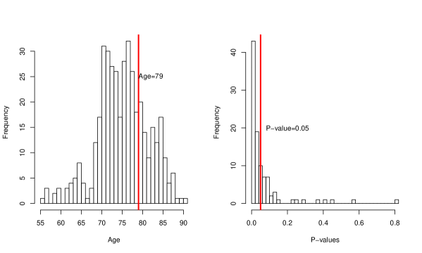
Figure 1: Left: Distribution of ages among the 410 subjects. Right: Empirical $p$-values for change point detection out of 50 random data splits.

Figure 1 (right) shows the empirical $p$-values for the 50 random data splits. Based on our results, 82% of the random splits with an estimated $p$-value lower than 0.05 have detected a change point. This strongly suggests that there is a change point in the linear structure due to the covariate age. Moreover, for the above 82% random splits, we record the estimated change points in Figure 2. We can see that in most cases, the argmax-based estimator identify the change point at the age of 79. The above analysis indicates that the linear structure between the MMSE score and MRI may be different before and after the age of 79. To see this more clearly, among the random splits with a change point, Figure 3 reports the features (with estimated coefficients bigger than 0.01) which are selected for more than 80% times before and after the change point, respectively. There are 16 features selected before the change point and 6 features selected after the change point. In other words, those 16 features shown in Figure 3 (left) are very predictive for the MMSE score for people with an age smaller or equal to 79. Once the age exceeds 79, it is better to predict the MMSE score using the other 6 features in Figure 3 (right). To verify this, for those random splits with a change point, we calculate the mean squared error for the corresponding testing data, based on the selected models using the training data. Figure 4 shows the results of our proposed method and lasso. We can see that our proposed method has better prediction performance by segmenting the model by the covariate age, with about 5.34% lower averaged MSE than that of lasso.

Lastly, as for the selected variables, some interesting observations can be made. For example, ROI 83 is predictive for the MMSE score across all ages. ROIs 30 and 69 are only very predictive for the MMSE score under the age of 79 and above 79, respectively. It is known that the 83th ROI corresponds to the amygdala region, and the 30th and 69th features correspond to the hippocampal regions. According to many previous studies (Zhang and Shen, 2012), those regions are known to be related to AD based on group comparison methods. For these and other selected features, it would be very interesting to investigate their relationship with AD by some group comparison studies according to the segmentation of ages.

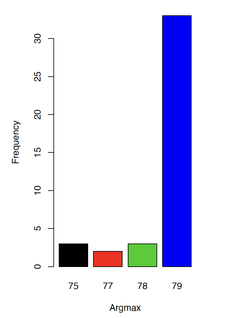
Figure 2: Estimated change points for the 82% random splits with change points among the 50 replications.

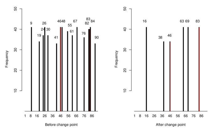
Figure 3: Frequency of features selected before the change point (left) and after the change point (right) for the ADNI data out of 50 random splits. Red corresponds to the features that are selected both before and after the change point.

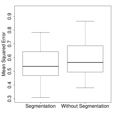
Figure 4: Mean squared errors for the prediction of the MMSE score with and without change point models.

6 Conclusions

In this paper, we propose a new method for change point inference in the context of high dimensional linear models. For any given subgroup $\mathcal{G}\subset\{1,\ldots,p\}$, a $L_{\infty}$-norm-based test statistic $T_{\mathcal{G}}$ is constructed for testing the homogeneity of regression coefficients across the observations. To approximate its limiting null distribution, a novel multiplier bootstrap procedure is introduced. Our new method is powerful against sparse alternatives with only a few entries in $\mathcal{G}$ having a change point, and allows the group size $|\mathcal{G}|$ to grow exponentially with the sample size $n$. As for the change point identification, a new change point estimator is obtained by taking “argmax” of the $L_{\infty}$-aggregated process $H_{\mathcal{G}}(t)$. Theoretically, the change point estimator is shown to be consistent, allowing the overall sparsity $s$ of regression coefficients and the group size $|\mathcal{G}|$ to grow simultaneously with the sample size $n$. In addition to single change point detection, we further combine our proposed method with the binary segmentation-based technique for detecting and identifying multiple change points. Our new testing method is relatively easy to implement and is justified via extensive numerical studies.

Supplementary Materials to “Simultaneous Change Point Detection and Identification for High Dimensional Linear Models”

Bin Liu , Xinsheng Zhang Yufeng Liu

The Appendix provides detailed proofs and additional results of the main paper. In Section A, we introduce some additional notations. In Section B, some additional numerical results, including size, power as well as detecting multiple change points, are provided. In Section C, some useful lemmas are provided. In Section D, we give the detailed proofs of theoretical results in the main paper. In Sections E and F, we prove the useful lemmas in Section C as well as the lemmas used in Section D.

Appendix A Some notations

Under $\mathbf{H}_{0}$, we set $\bm{\beta}^{(0)}:=\bm{\beta}^{(1)}=\bm{\beta}^{(2)}$ and $s^{(0)}:=s^{(1)}=s^{(2)}$. We set $s:=s^{(1)}\vee s^{(2)}$. For a given subgroup $\mathcal{G}$, set $\Pi_{\mathcal{G}}=\{j\in\mathcal{G}:\beta^{(1)}_{j}-\beta^{(2)}_{j}\neq 0\}$ as the subset of coordinates with a change point. For a vector $\bm{v}\in\mathbb{R}^{p}$, we set $\mathcal{M}(\bm{v})$ as the number of non-zero elements of $\bm{v}$, i.e. $\mathcal{M}(\bm{v})=\sum_{j=1}^{p}\mathbf{1}\{v_{j}\neq 0\}$. We denote $J(\bm{v})=\{1\leq j\leq p:v_{j}\neq 0\}$ as the set of non-zero elements of $\bm{v}$. For a set $J$ and $\bm{v}\in\mathbb{R}^{p}$, denote $\bm{v}_{J}$ as the vector in $\mathbb{R}^{p}$ that has the same coordinates as $\bm{v}$ on $J$ and zero coordinates on the complement $J^{c}$ of $J$. Denote $\mathcal{X}=\{\mathbf{X},\bm{Y}\}$. We use $C_{1},C_{2},\ldots$ to denote constants that may vary from line to line.

Appendix B Additional numerical results

B.1 Implementations of the existing techniques

Before reporting additional numerical results, we first demonstrate how to implement the mentioned techniques in this paper.

Implementation of the existing methods: For Lee2016, we use the package-glmnet to implement their proposed algorithm. Note that Lee2016 involves a selection of the tuning parameter $\lambda$. For each replication, we generate a sequence from $2^{-5}$ to $2^{5}$ and select the “best” $\lambda$ by 10-fold cross-validation. For L&B, we use the binary segmentation-based method with parameters suggested by the authors using the package-glmnet. Moreover, we use a three folded cross-validation procedure to select the tuning parameters in L&B. For VPWBS, we implement the algorithm using the codes provided by the authors at GitHub (https://github.com/darenwang/VPBS). For SGL, we use the package-SGL with parameters in favor of their method and use three folded cross-validation to select the tuning parameters. Note that SGL solves the following optimization problem:

$$\begin{array}[]{ll}\{\widehat{\bm{\beta}}_{1},\ldots,\widehat{\bm{\beta}}_{n}\}\\ =\mathop{\text{\rm arg\,min}}\limits_{\bm{\beta}_{1},\ldots,\bm{\beta}_{n}\in\mathbb{R}^{p}}\sum\limits_{i=1}^{n}(Y_{i}-\bm{X}_{i}^{\top}\bm{\beta}_{i})^{2}+\lambda_{n}\alpha\sum\limits_{i=1}^{n}\|\bm{\beta}_{i}-\bm{\beta}_{i-1}\|_{2}+\lambda_{n}(1-\alpha)\sum\limits_{i=1}^{n}\|\bm{\beta}_{i}-\bm{\beta}_{i-1}\|_{1}.\end{array}$$

Based on the above optimization, SGL finds a change point at $i^{*}$ if $\widehat{\bm{\beta}}_{i^{*}}-\widehat{\bm{\beta}}_{i^{*}-1}\neq\mathbf{0}$. It is well-known that lasso tends to over select the variables. In addition, SGL essentially solves a group lasso problem by calculating $n\times p$ parameters using only $n$ observations. As a result, SGL may yield false alarms by identifying some $\{i:\bm{\beta}_{i}-\bm{\beta}_{i-1}=\mathbf{0}_{p}\}$ as a change point. This can be seen by our following empirical size performance in Section 4.1 as well as the multiple change point detection results in Section 4.3. Moreover, we note that this phenomenon was also observed by Wang et al. (2021).

Implementation of our method: As for our proposed method, we use the package-hdi to obtain the node-wise lasso estimator $\widehat{\bm{\Theta}}$. Note that the calculation of the lasso processes $\widehat{\bm{\beta}}^{(0,t)}$ and $\widehat{\bm{\beta}}^{(t,1)}$ with $t\in[\tau_{0},1-\tau_{0}]$ involves the selection of tuning parameters $\lambda_{1}(t)$ and $\lambda_{2}(t)$ defined in (2.7). We select the tuning parameters via three folded cross-validation. Specifically, for each search location $t\in[\tau_{0},1-\tau_{0}]$, we set

$$\lambda_{1}(t)=C\sqrt{\dfrac{\log(p)}{\lfloor nt\rfloor}},~{}~{}\text{and}~{}~{}\lambda_{2}(t)=C\sqrt{\dfrac{\log(p)}{\lfloor nt\rfloor^{*}}},~{}~{}\text{with}~{}C\in\{1,2,\ldots,8\}.$$

Then, we use the package-glmnet to select the best “C” via three folded cross-validation, which enjoys satisfactory performance in change point detection and identification.

B.2 Additional size performance

In addition to $N(0,1)$, we also report the size performance under standardized $\rm Gamma(4,1)$ (Table 5) and Student’s $t_{5}$ (Table 6) distributions which have very similar performance to Table 1 of the main paper. In this case, our proposed method can control the size under the nominal level. This suggests that the bootstrap null distribution is correctly calibrated even for non-normal underlying errors.

B.3 Additional power performance

Table 7 shows the power performance for Model 2 with banded covariance structures of $\bm{X}$, which is similar to Table 2 in the main paper.

B.4 Computational cost

In this section, we compare the computational cost of the existing methods. In theory, for detecting a single change point, the computational costs for the existing methods are $O(n\text{Lasso}(n,p))$ (Lee2016), $O(n\text{Lasso}(n,p))$ (L&B), $O(Mn\text{GroupLasso}(n,p))$ (VPWBS), $O(\text{GroupLasso}(n,np))$ (SGL), and $(B+1)O(n\text{Lasso}(n,p))$ (our proposed method), where $\text{Lasso}(n,p)$ and $\text{GroupLasso}(n,p)$ denote the computational cost for solving lasso and group lasso problems with the sample size $n$ and the data dimension $p$, $M$ is the number of random intervals in Wang et al. (2021), and $B$ is the number of bootstrap replications. Empirically, we implement the corresponding program independently on a CPU (Linux) with 2.50GHz and 256G RAM and report the average computational time (seconds) based on 5 replications. Note that the computational cost for our proposed method mainly relies on the bootstrap procedure which can be time-consuming. Since the $B$ bootstrap replications can be done separately, we can use parallel computation in modern computer techniques to further reduce the computational time via implementing the $B$ bootstrap replications in a parallel fashion on different cores of the Linux server. Specifically, for our method, we report the computational cost by using 8, 16, and 32 logical cores, respectively. Figure 5 reports the computational time for the existing methods with various $n\in\{200,400,600,800,1000\}$ (upper) and $p\in\{100,200,300,400\}$ (bottom). In general, Lee2016 and L&B are the most efficient and have very close performance. The computational time for SGL is the most expensive among all methods. For our proposed algorithm, we can see that it has a tolerable computational cost and can even be comparable to its competitors using more cores. Lastly, Figure 5 shows that for all methods, the computational time grows linearly with $n$ and $p$, and it appears that the computational cost is more sensitive to the growth of the sample size $n$ than the data dimension $p$.

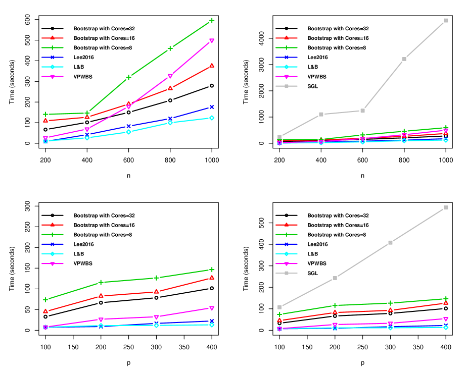
Figure 5: Computational time (seconds) for the existing methods based on an average of 5 replications. Upper: Computational time for $p=200$ and $n\in\{200,400,600,800,1000\}$ without the plot of SGL (left) and with SGL (right), respectively. Bottom: Computational time for $n=200$ and $p\in\{100,200,300,400\}$ without the plot of SGL (left) and with SGL (right), respectively.

Table 5: Empirical sizes for Models 1 and 2 under various combinations of $(n,p,s)$. The errors are generated from standardized Gamma(4,1) distributions. The results are based on 2000 replications.

Empirical sizes (%) for Gamma(4,1) with $(n,s)=(200,5)$
Model	$\mathcal{G}$	$p$	Boot-I ($\alpha=1\%$)	Boot-II ($\alpha=1\%$)	Boot-I ($\alpha=5\%$)	Boot-II ($\alpha=5\%$)	SGL	L&B
$\bm{\Sigma}=\mathbf{I}$	${\mathcal{S}}$	100	7.00	1.70	14.81	4.63	NA	NA
		200	8.64	1.29	17.70	4.32	NA	NA
		300	9.67	2.11	16.67	5.14	NA	NA
		400	13.99	1.80	23.66	5.14	NA	NA
	${\mathcal{S}}^{c}$	100	4.32	0.98	9.67	3.60	NA	NA
		200	6.38	1.23	15.02	3.81	NA	NA
		300	11.11	1.08	20.99	3.86	NA	NA
		400	13.58	1.80	24.90	4.27	NA	NA
	${\mathcal{S}}\cup{\mathcal{S}}^{c}$	100	6.17	1.49	15.43	4.73	56.67	0.00
		200	9.05	1.54	17.28	3.96	43.33	0.00
		300	10.91	1.44	23.25	4.22	40.00	0.00
		400	18.31	2.11	30.66	4.94	40.00	0.00
$\bm{\Sigma}=\bm{\Sigma}^{*}$	${\mathcal{S}}$	100	4.94	1.92	11.73	4.87	NA	NA
		200	6.79	1.58	15.64	4.46	NA	NA
		300	8.23	2.12	17.90	5.81	NA	NA
		400	12.55	2.06	24.07	4.65	NA	NA
	${\mathcal{S}}^{c}$	100	3.91	1.44	10.08	4.03	NA	NA
		200	3.70	1.57	10.29	3.82	NA	NA
		300	7.61	1.30	14.61	3.69	NA	NA
		400	4.73	0.89	15.84	2.73	NA	NA
	${\mathcal{S}}\cup{\mathcal{S}}^{c}$	100	8.64	1.36	16.87	3.35	51.11	0.00
		200	7.00	1.37	12.96	3.14	40.00	0.00
		300	8.02	1.36	19.55	3.14	50.00	0.00
		400	7.20	1.16	15.02	3.76	37.78	0.00

Table 6: Empirical sizes for Models 1 and 2 under various combinations of $(n,p,s)$. The errors are generated from standardized Student’s $t_{5}$ distributions. The results are based on 2000 replications.

Empirical sizes (%) for Student’s $t_{5}$ with $(n,s)=(200,5)$
Model	$\mathcal{G}$	$p$	Boot-I ($\alpha=1\%$)	Boot-II ($\alpha=1\%$)	Boot-I ($\alpha=5\%$)	Boot-II ($\alpha=5\%$)	SGL	L&B
$\bm{\Sigma}=\mathbf{I}$	${\mathcal{S}}$	100	5.35	1.29	15.23	4.17	NA	NA
		200	9.26	1.95	21.40	5.61	NA	NA
		300	9.05	1.95	20.16	5.30	NA	NA
		400	14.40	2.37	22.84	6.43	NA	NA
	${\mathcal{S}}^{c}$	100	5.97	1.18	10.29	4.22	NA	NA
		200	9.67	1.59	20.99	4.42	NA	NA
		300	10.70	2.16	22.22	4.78	NA	NA
		400	11.93	1.85	21.60	4.48	NA	NA
	${\mathcal{S}}\cup{\mathcal{S}}^{c}$	100	7.20	1.65	16.05	4.63	61.11	0.00
		200	10.29	1.80	20.78	4.68	45.56	0.00
		300	12.76	1.75	26.13	5.20	50.00	0.00
		400	16.46	2.42	30.45	5.04	54.44	0.00
$\bm{\Sigma}=\bm{\Sigma}^{*}$	${\mathcal{S}}$	100	6.17	1.33	13.58	3.90	NA	NA
		200	9.05	1.89	18.31	5.38	NA	NA
		300	9.05	2.72	18.31	5.78	NA	NA
		400	10.91	2.04	21.19	5.32	NA	NA
	${\mathcal{S}}^{c}$	100	4.53	1.48	10.29	4.35	NA	NA
		200	3.91	1.64	10.08	4.26	NA	NA
		300	6.79	1.44	14.40	3.65	NA	NA
		400	7.61	1.80	16.46	4.41	NA	NA
	${\mathcal{S}}\cup{\mathcal{S}}^{c}$	100	6.79	1.64	13.58	5.19	51.11	0.00
		200	5.14	1.59	12.96	4.41	44.44	0.00
		300	9.26	2.10	18.11	4.87	31.11	0.00
		400	9.47	2.05	18.93	4.87	36.67	0.00

Table 7: Empirical powers (%) for Case 1 under Model 2 with various dimensions, candidate subgroups, and change point locations. The sample size is $n=200$. The significance level is $\alpha=5\%$. The numerical results are based on 2000 replications.

Empirical powers (%) with $\bm{\delta}=0.5\sqrt{{\log(p)}/{n}}\times(2^{3},2^{2},2^{1},2^{0},2^{-1})$.
			Change point at $k^{*}=0.5n$			Change point at $k^{*}=0.3n$
Model	$\mathcal{G}$	$p$	Boot-II	L&B		Boot-II	L&B
$\bm{\Sigma}=\bm{\Sigma}^{*}$	${\mathcal{S}}$	200	49.33	NA		30.27	NA
		400	45.33	NA		33.33	NA
	${\mathcal{S}}^{c}$	200	1.67	NA		3.00	NA
		400	2.67	NA		1.83	NA
	${\mathcal{S}}\cup{\mathcal{S}}^{c}$	200	34.00	0.00		21.43	0.00
		400	28.00	0.00		18.67	0.00
Empirical powers (%) with $\bm{\delta}=\sqrt{{\log(p)}/{n}}\times(2^{3},2^{2},2^{1},2^{0},2^{-1})$.
			Change point at $k^{*}=0.5n$			Change point at $k^{*}=0.3n$
Model	$\mathcal{G}$	$p$	Boot-II	L&B		Boot-II	L&B
$\bm{\Sigma}=\bm{\Sigma}^{*}$	${\mathcal{S}}$	200	100.00	NA		99.18	NA
		400	100.00	NA		99.18	NA
	${\mathcal{S}}^{c}$	200	2.06	NA		2.67	NA
		400	2.06	NA		1.65	NA
	${\mathcal{S}}\cup{\mathcal{S}}^{c}$	200	99.59	60.42		97.53	40.63
		400	99.18	57.29		95.68	47.92
Empirical powers (%) with $\bm{\delta}=2\sqrt{{\log(p)}/{n}}\times(2^{3},2^{2},2^{1},2^{0},2^{-1})$.
			Change point at $k^{*}=0.5n$			Change point at $k^{*}=0.3n$
Model	$\mathcal{G}$	$p$	Boot-II	L&B		Boot-II	L&B
$\bm{\Sigma}=\bm{\Sigma}^{*}$	${\mathcal{S}}$	200	100.00	NA		100.00	NA
		400	100.00	NA		100.00	NA
	${\mathcal{S}}^{c}$	200	2.67	NA		1.82	NA
		400	2.26	NA		1.65	NA
	${\mathcal{S}}\cup{\mathcal{S}}^{c}$	200	100.00	100.00		100.00	99.49
		400	100.00	100.00		100.00	99.49

Appendix C Useful lemmas

Let $\bm{Z}_{1},\ldots,\bm{Z}_{n}$ be independent centered random vectors in $\mathbb{R}^{p}$ with $\bm{Z}_{i}=(Z_{i,1},\ldots,Z_{i,p})^{\top}$ for $i=1,\ldots,n$. Let $\bm{G}_{1},\ldots,\bm{G}_{n}$ be independent centered Gaussian random vectors in $\mathbb{R}^{p}$ such that each $\bm{G}_{i}$ has the same covariance matrix as $\bm{Z}_{i}$. We then require the following conditions:

(M1)

There is a constant $b>0$ such that $\inf_{1\leq j\leq p}{\mathbb{E}}(Z_{i,j})^{2}\geq b$ for $i=1,\ldots,n$.

(M2)

There exists a constant $K>0$ such that $\max\limits_{1\leq j\leq p}\dfrac{1}{n}\sum\limits_{i=1}^{n}{\mathbb{E}}|Z_{i,j}|^{2+\ell}\leq K^{\ell}$ for $\ell=1,2$.

(M3)

There exists a constant $K^{\prime}>0$ such that ${\mathbb{E}}\big{(}\exp(|Z_{i,j}|/K^{\prime})\big{)}\leq 2$ for $j=1,\ldots,d$ and $i=1,\ldots,n$.

Lemma C.1.

(Liu et al. (2020)) Assume that $\log(pn)=O(\lfloor n\tau_{0}\rfloor^{\zeta})$ holds for some $0<\zeta<1/7$. Let

$$\bm{S}^{\bm{Z}}(\lfloor nt\rfloor)=\dfrac{1}{\sqrt{n}}\sum_{i=1}^{n}\bm{Z}_{i}\big{(}\mathbf{1}(i\leq\lfloor nt\rfloor)-\lfloor nt\rfloor/n\big{)},~{}~{}\bm{S}^{\bm{G}}(\lfloor nt\rfloor)=\dfrac{1}{\sqrt{n}}\sum_{i=1}^{n}\bm{G}_{i}\big{(}\mathbf{1}(i\leq\lfloor nt\rfloor)-\lfloor nt\rfloor/n\big{)}$$

be the partial sum processes for $(\bm{Z}_{i})_{i\geq 1}$ and $(\bm{G}_{i})_{i\geq 1}$, respectively. If $\bm{Z}_{1},\ldots,\bm{Z}_{n}$ satisfy $\bf(M1)$, $\bf(M2)$ and $\bf(M3)$, then there is a constant $\zeta_{0}>0$ such that

$$\sup_{z\in(0,\infty)}\big{|}{\mathbb{P}}(\max_{\tau_{0}\leq t\leq 1-\tau_{0}}\|\bm{S}^{\bm{Z}}(\lfloor nt\rfloor)\|_{\infty}\leq z\big{)}-{\mathbb{P}}(\sup_{\tau_{0}\leq t\leq 1-\tau_{0}}\|\bm{S}^{\bm{G}}(\lfloor nt\rfloor)\|_{\infty}\leq z\big{)}\big{|}\leq Cn^{-\zeta_{0}},$$ (C.1)

where $C$ is a constant only depending on $b$, $K$, and $K^{\prime}$.

Lemma C.2 (Nazarovs inequality in Nazarov (2003)).

Let $\bm{W}=(W_{1},W_{2},\cdots,W_{p})^{\top}\in\mathbb{R}^{p}$ be centered Gaussian random vector with $\inf_{1\leq k\leq p}{\mathbb{E}}(W_{k})^{2}\geq b>0$. Then for any $\bm{x}\in\mathbb{R}^{p}$ and $a>0$, we have

$${\mathbb{P}}(\bm{W}\leq\bm{x}+a)-{\mathbb{P}}(\bm{W}\leq\bm{x})\leq Ca\sqrt{\log p},$$

where $C$ is a constant only depending on $b$.

Lemma C.3.

(Zhou et al. (2018)) Let $\bm{W}=(W_{1},\ldots,W_{p})^{\top}$ be a random vector with a marginal distribution $N(0,\sigma_{i}^{2})$ ($1\leq i\leq p$). Suppose $\exists A_{0}>0$ such that $\max_{i}\sigma_{i}^{2}\leq A^{2}_{0}$. Then, for any $t>0$, we have

$${\mathbb{E}}\big{(}\max_{1\leq i\leq p}|W_{i}|\big{)}\leq\dfrac{\log(2p)}{t}+\dfrac{tA_{0}^{2}}{2}.$$

Lemma C.4 (Van de Geer et al. (2014)).

Suppose Assumptions $\mathbf{(A.1)}$ – $\mathbf{(A.3)}$ hold. Assume additionally $\max_{j}\sqrt{s_{j}\log(p)/n}=o(1)$ holds. For the node-wise regression in (2.3), choosing the tuning parameters $\lambda_{(j)}\approx\sqrt{\log(p)/n}$ uniformly over $j$, we have

$$\begin{array}[]{l}\|\widehat{\bm{\Theta}}_{j}-\bm{\Theta}_{j}\|_{q}=O_{p}\Big{(}s_{j}^{1/q}\sqrt{\dfrac{\log(p)}{n}}\Big{)},~{}\text{for}~{}q=1,2.\\ \end{array}$$ (C.2)

Lemma C.5.

Let $\bm{Z}_{1},\ldots,\bm{Z}_{n}$ be independent centered random vectors in $\mathbb{R}^{p}$ with $\bm{Z}_{i}=(Z_{i,1},\ldots$ $,Z_{i,p})^{\top}$ for $i=1,\ldots,n$. Assume that $\mathbf{Z}_{i}$ follows the sub-exponential distribution. Then, for any given subgroup $\mathcal{G}\subset\{1,\ldots,p\}$, with probability at least $1-C_{1}(pn)^{-C_{2}}$, we have

$$\max_{t\in[\tau_{0},1-\tau_{0}]}\max\limits_{j\in\mathcal{G}}\Big{|}\dfrac{1}{\sqrt{n}}\Big{(}\sum_{i=1}^{\lfloor nt\rfloor}Z_{i,j}-\dfrac{\lfloor nt\rfloor}{n}\sum_{i=1}^{n}Z_{i,j}\Big{)}\Big{|}\leq C_{3}\sqrt{\log(|\mathcal{G}|n)},$$ (C.3)

where $C_{1}$, $C_{2}$, and $C_{3}$ are universal positive constants not depending on $p$ or $n$.

We next provide some useful results for the lasso estimators from heterogeneous data observations. To this end, for each $t\in[\tau_{0},1-\tau_{0}]$, define

$$\begin{array}[]{ll}\mathcal{A}(t)=\left\{\Big{\|}\dfrac{1}{\lfloor nt\rfloor}\big{(}\mathbf{X}_{(0,t)})^{\top}(\bm{Y}_{(0,t)}-\mathbf{X}_{(0,t)}\bm{\beta}^{(0,t)}\Big{\|}_{\infty}\leq\lambda^{(1)}\right\},\\ \\ \mathcal{B}(t)=\left\{\Big{\|}\dfrac{1}{\lfloor nt\rfloor^{*}}\big{(}\mathbf{X}_{(t,1)})^{\top}(\bm{Y}_{(t,1)}-\mathbf{X}_{(t,1)}\bm{\beta}^{(t,1)}\Big{\|}_{\infty}\leq\lambda^{(2)}\right\},\\ \\ \end{array}$$ (C.4)

where $\lambda^{(1)}:=K_{1}\sqrt{\dfrac{\log(p)}{\lfloor nt\rfloor}}$ and $\lambda^{(2)}:=K_{2}\sqrt{\dfrac{\log(p)}{\lfloor nt\rfloor^{*}}}$, and $K_{1},\ldots,K_{2}$ are some universal positive constants not depending on $n$ or $p$.

The following Lemma C.6 provides a basic inequality for the lasso estimators, which is important for deriving the precise estimation error bound as well as prediction error bound (see Lemma C.8 below). The proof of Lemma C.6 is given in Section F.2.

Lemma C.6.

Suppose Assumptions $\mathbf{(A.1)}$ – $\mathbf{(A.3)}$ hold. Assume $\|\bm{\beta}^{(2)}-\bm{\beta}^{(1)}\|_{2}\leq C_{\bm{\Delta}}$ for some $C_{\bm{\Delta}}>0$. Recall $\bm{\beta}^{(0,t)}$ and $\bm{\beta}^{(t,1)}$ defined in (2.5). Let $\widehat{\bm{\beta}}^{(0,t)}$ and $\widehat{\bm{\beta}}^{(t,1)}$ be the lasso estimators as defined in (2.7). Then, for each $t\in[\tau_{0},1-\tau_{0}]$, under the event $\mathcal{A}(t)\cap\mathcal{B}(t)$, we have

$$\dfrac{\big{\|}\mathbf{X}_{(0,t)}\big{(}\widehat{\bm{\beta}}^{(0,t)}-\bm{\beta}^{(0,t)}\big{)}\big{\|}_{2}^{2}}{\lfloor nt\rfloor}+\lambda_{1}(t)\big{\|}(\widehat{\bm{\beta}}^{(0,t)}-\bm{\beta}^{(0,t)})_{J^{c}(\bm{\beta}^{(0,t)})}\big{\|}_{1}\leq 3\lambda_{1}(t)\big{\|}(\widehat{\bm{\beta}}^{(0,t)}-\bm{\beta}^{(0,t)})_{J(\bm{\beta}^{(0,t)})}\big{\|}_{1},$$ (C.5)

and

$$\dfrac{\big{\|}\mathbf{X}_{(t,1)}\big{(}\widehat{\bm{\beta}}^{(t,1)}-\bm{\beta}^{(t,1)}\big{)}\big{\|}_{2}^{2}}{\lfloor nt\rfloor^{*}}+\lambda_{2}(t)\big{\|}(\widehat{\bm{\beta}}^{(t,1)}-\bm{\beta}^{(t,1)})_{J^{c}(\bm{\beta}^{(t,1)})}\big{\|}_{1}\leq 3\lambda_{2}(t)\big{\|}(\widehat{\bm{\beta}}^{(t,1)}-\bm{\beta}^{(t,1)})_{J(\bm{\beta}^{(t,1)})}\big{\|}_{1},$$ (C.6)

where $\lambda_{1}(t):=2\lambda^{(1)}$, $\lambda_{2}(t):=2\lambda^{(2)}$.

The following Lemma C.7 provides the estimation error bounds for the lasso estimators $\widehat{\bm{\beta}}^{(0,t)}$ and $\widehat{\bm{\beta}}^{(t,1)}$ in terms of $\ell_{q}$-norm. The proof of Lemma C.7 is given in Section F.3.

Lemma C.7.

Suppose Assumptions $\mathbf{(A.1)}$ – $\mathbf{(A.3)}$ hold. Assume $\|\bm{\beta}^{(2)}-\bm{\beta}^{(1)}\|_{2}\leq C_{\bm{\Delta}}$ for some $C_{\bm{\Delta}}>0$. Recall $\bm{\beta}^{(0,t)}$ and $\bm{\beta}^{(t,1)}$ defined in (2.5). Let $\widehat{\bm{\beta}}^{(0,t)}$ and $\widehat{\bm{\beta}}^{(t,1)}$ be the lasso estimators as defined in (2.7). For each $t\in[\tau_{0},1-\tau_{0}]$, let $s_{1}(t):=\mathcal{M}(\bm{\beta}^{(0,t)})$ and $s_{2}(t):=\mathcal{M}(\bm{\beta}^{(t,1)})$. Then, under the event $\mathcal{A}(t)\cap\mathcal{B}(t)$, we have

$$\begin{array}[]{l}\big{\|}\widehat{\bm{\beta}}^{(0,t)}-\bm{\beta}^{(0,t)}\big{\|}_{q}\leq C_{1}(s_{1}(t))^{\frac{1}{q}}\sqrt{\dfrac{\log p}{\lfloor nt\rfloor}},~{}~{}\big{\|}\widehat{\bm{\beta}}^{(t,1)}-\bm{\beta}^{(t,1)}\big{\|}_{q}\leq C_{2}(s_{2}(t))^{\frac{1}{q}}\sqrt{\dfrac{\log p}{\lfloor nt\rfloor^{*}}},~{}q=1,2,\\ \\ \dfrac{\big{\|}\mathbf{X}_{(0,t)}\big{(}\widehat{\bm{\beta}}^{(0,t)}-\bm{\beta}^{(0,t)}\big{)}\big{\|}_{2}^{2}}{\lfloor nt\rfloor}\leq C_{3}s_{1}(t)\dfrac{\log p}{\lfloor nt\rfloor},~{}~{}\dfrac{\big{\|}\mathbf{X}_{(t,1)}\big{(}\widehat{\bm{\beta}}^{(t,1)}-\bm{\beta}^{(t,1)}\big{)}\big{\|}_{2}^{2}}{\lfloor nt\rfloor^{*}}\leq C_{4}s_{2}(t)\dfrac{\log p}{\lfloor nt\rfloor^{*}},\\ \\ \mathcal{M}(\widehat{\bm{\beta}}^{(0,t)})\leq C_{5}s_{1}(t),~{}~{}~{}~{}\mathcal{M}(\widehat{\bm{\beta}}^{(t,1)})\leq C_{6}s_{2}(t),\end{array}$$ (C.7)

where $C_{1},\ldots,C_{6}$ are some universal positive constants not depending on $n$ or $p$.

Lastly, as a by product of Lemma C.7, the following Lemma C.8 provides the estimation error bounds for $\widehat{\bm{\beta}}^{(0,t)}-\bm{\beta}^{(1)}$ and $\widehat{\bm{\beta}}^{(t,1)}-\bm{\beta}^{(2)}$ in terms of the $\ell_{q}$-norm, which is frequently used in the proofs.

Lemma C.8.

Suppose Assumptions $\mathbf{(A.1)}$ – $\mathbf{(A.3)}$ hold. Assume $\|\bm{\beta}^{(2)}-\bm{\beta}^{(1)}\|_{2}\leq C_{\bm{\Delta}}$ for some $C_{\bm{\Delta}}>0$. Recall $s:=s^{(1)}\vee s^{(2)}$. Let $\widehat{\bm{\beta}}^{(0,t)}$ and $\widehat{\bm{\beta}}^{(t,1)}$ be the lasso estimators as defined in (2.7). Then, under the event $\mathcal{A}(t)\cap\mathcal{B}(t)$, for each $t\in[\tau_{0},1-\tau_{0}]$, we have

$$\begin{array}[]{l}\big{\|}\widehat{\bm{\beta}}^{(0,t)}-\bm{\beta}^{(1)}\big{\|}_{q}\leq C_{1}\max\Big{\{}s^{\frac{1}{q}}\sqrt{\dfrac{\log p}{\lfloor nt\rfloor}},\dfrac{\lfloor nt\rfloor-\lfloor nt_{0}\rfloor}{\lfloor nt\rfloor}\big{\|}\bm{\beta}^{(2)}-\bm{\beta}^{(1)}\big{\|}_{q}\mathbf{1}\{t\geq t_{0}\}\Big{\}},q=1,2,\\ \\ \big{\|}\widehat{\bm{\beta}}^{(t,1)}-\bm{\beta}^{(2)}\big{\|}_{q}\leq C_{2}\max\Big{\{}s^{\frac{1}{q}}\sqrt{\dfrac{\log p}{\lfloor nt\rfloor^{*}}},\dfrac{\lfloor nt_{0}\rfloor-\lfloor nt\rfloor}{\lfloor nt\rfloor^{*}}\big{\|}\bm{\beta}^{(2)}-\bm{\beta}^{(1)}\big{\|}_{q}\mathbf{1}\{t\leq t_{0}\}\Big{\}},q=1,2,\\ \\ \dfrac{\big{\|}\mathbf{X}_{(0,t)}\big{(}\widehat{\bm{\beta}}^{(0,t)}-\bm{\beta}^{(1)}\big{)}\big{\|}_{2}^{2}}{\lfloor nt\rfloor}\leq C_{3}\max\Big{\{}s\dfrac{\log p}{\lfloor nt\rfloor},\big{(}\dfrac{\lfloor nt\rfloor-\lfloor nt_{0}\rfloor}{\lfloor nt\rfloor}\big{)}^{2}\big{\|}\bm{\beta}^{(2)}-\bm{\beta}^{(1)}\big{\|}_{2}^{2}\mathbf{1}\{t\geq t_{0}\}\Big{\}},\\ \\ \dfrac{\big{\|}\mathbf{X}_{(t,1)}\big{(}\widehat{\bm{\beta}}^{(t,1)}-\bm{\beta}^{(2)}\big{)}\big{\|}_{2}^{2}}{\lfloor nt\rfloor^{*}}\leq C_{4}\max\Big{\{}s\dfrac{\log p}{\lfloor nt\rfloor^{*}},\big{(}\dfrac{\lfloor nt_{0}\rfloor-\lfloor nt\rfloor}{\lfloor nt\rfloor^{*}})^{2}\big{\|}\bm{\beta}^{(2)}-\bm{\beta}^{(1)}\big{\|}_{2}^{2}\mathbf{1}\{t\leq t_{0}\}\Big{\}},\\ \\ \mathcal{M}(\widehat{\bm{\beta}}^{(0,t)})\leq C_{5}s,~{}~{}~{}~{}\mathcal{M}(\widehat{\bm{\beta}}^{(t,1)})\leq C_{6}s,\end{array}$$ (C.8)

where $C_{1},\ldots,C_{6}$ are some universal positive constants not depending on $n$ or $p$.

The following Lemma C.9 shows that the results in Lemmas C.6 – C.8 occur uniformly over $t\in[\tau_{0},1-\tau_{0}]$ with high probability. The proof of Lemma C.9 is given in Section F.4.

Lemma C.9.

Suppose Assumptions $\mathbf{(A.1)}$ – $\mathbf{(A.3)}$ hold. Assume $\|\bm{\beta}^{(2)}-\bm{\beta}^{(1)}\|_{2}\leq C_{\bm{\Delta}}$ for some $C_{\bm{\Delta}}>0$. Then we have

$${\mathbb{P}}\big{(}\bigcap_{t\in[\tau_{0},1-\tau_{0}]}\big{\{}\mathcal{A}(t)\cap\mathcal{B}(t)\big{\}}\big{)}\geq 1-C_{1}(np)^{-C_{2}},$$ (C.9)

where $C_{1},C_{2}$ are some big enough universal positive constants not depending on $n$ or $p$.

Appendix D Proof of main results

D.1 Proof of Proposition 3.1

Proof.

Note that the proof of Part (i) is easier than Part (ii). To save space, we give the proof of Part (ii). Firstly, we consider $\mathcal{R}_{1}(s,3,\mathbb{T})$. The proof proceeds in two steps.
Step 1: we prove $\sup_{t\in[\tau_{0},1-\tau_{0}]}\|\widehat{\bm{\Sigma}}_{(0,t)}-\bm{\Sigma}\|_{\infty}=O_{p}(\sqrt{\log(p)/\lfloor n\tau_{0}\rfloor})$. For any fixed $t\in[\tau_{0},1-\tau_{0}]$ and $j,k\in\{1,\ldots,p\}$, by Assumption (A.1), using exponential inequality, we have

$${\mathbb{P}}\big{(}|\dfrac{1}{\lfloor nt\rfloor}\sum_{i=1}^{\lfloor nt\rfloor}(X_{ij}X_{ik}-{\mathbb{E}}[X_{ij}X_{ik}])|\geq x\big{)}\leq C_{1}\exp(-C_{2}\lfloor nt\rfloor x^{2})\leq C_{1}\exp(-C_{2}\lfloor n\tau_{0}\rfloor x^{2}).$$

Hence, taking $x=C_{3}\sqrt{\log(pn)/\lfloor n\tau_{0}\rfloor}$ for some big constant $C_{3}>0$, we have:

$${\mathbb{P}}\big{(}|\dfrac{1}{\lfloor nt\rfloor}\sum_{i=1}^{\lfloor nt\rfloor}(X_{ij}X_{ik}-{\mathbb{E}}[X_{ij}X_{ik}])|\geq x\big{)}\leq C_{1}(np)^{-C_{3}}.$$

As a result, we have:

$$\begin{array}[]{ll}{\mathbb{P}}(\sup\limits_{t\in[\tau_{0},1-\tau_{0}]}\|\widehat{\bm{\Sigma}}_{(0,t)}-\bm{\Sigma}\|_{\infty}\geq x)\\ ={\mathbb{P}}\Big{(}\bigcup\limits_{t}\bigcup\limits_{j,k}\big{\{}|\dfrac{1}{\lfloor nt\rfloor}\sum\limits_{i=1}^{\lfloor nt\rfloor}(X_{ij}X_{ik}-{\mathbb{E}}[X_{ij}X_{ik}])|\geq x\big{\}}\Big{)}\\ \leq np^{2}\max_{t,j,k}{\mathbb{P}}\big{(}|\dfrac{1}{\lfloor nt\rfloor}\sum\limits_{i=1}^{\lfloor nt\rfloor}(X_{ij}X_{ik}-{\mathbb{E}}[X_{ij}X_{ik}])|\geq x\big{)}\\ \leq C_{1}(np)^{-C_{4}},\end{array}$$

where $C_{1}-C_{4}$ are some big enough universal constants. This yields $\sup_{t\in[\tau_{0},1-\tau_{0}]}\|\widehat{\bm{\Sigma}}_{(0,t)}-\bm{\Sigma}\|_{\infty}=O_{p}(\sqrt{\log(p)/\lfloor n\tau_{0}\rfloor})$.
Step 2: For integers $s$ such that $1\leq s\leq p$, a set of indices $J_{0}\subset\{1,\ldots,p\}$ with $|J_{0}|\leq s$, and any vector $\bm{\delta}$ satisfying $\|\bm{\delta}_{J_{0}^{c}}\|_{1}\leq 3\|\bm{\delta}_{J_{0}}\|_{1}$, we have:

$$\begin{array}[]{rl}\dfrac{\bm{\delta}^{\top}\widehat{\bm{\Sigma}}_{(0,t)}\bm{\delta}}{|\bm{\delta}_{J_{0}}|_{2}^{2}}&=_{(1)}\dfrac{\bm{\delta}^{\top}\bm{\Sigma}\bm{\delta}}{|\bm{\delta}_{J_{0}}|_{2}^{2}}+\dfrac{\bm{\delta}^{\top}(\bm{\Sigma}-\widehat{\bm{\Sigma}}_{(0,t)})\bm{\delta}}{|\bm{\delta}_{J_{0}}|_{2}^{2}},\\ &\geq_{(2)}\dfrac{\bm{\delta}^{\top}\bm{\Sigma}\bm{\delta}}{|\bm{\delta}_{J_{0}}|_{2}^{2}}-\dfrac{\sup_{t\in[\tau_{0},1-\tau_{0}]}\|\widehat{\bm{\Sigma}}_{(0,t)}-\bm{\Sigma}\|_{\infty}}{|\bm{\delta}_{J_{0}}|_{2}^{2}}|\bm{\delta}|_{1}^{2},\\ &\geq_{(3)}\dfrac{\bm{\delta}^{\top}\bm{\Sigma}\bm{\delta}}{|\bm{\delta}_{J_{0}}|_{2}^{2}}-\dfrac{\sup_{t\in[\tau_{0},1-\tau_{0}]}\|\widehat{\bm{\Sigma}}_{(0,t)}-\bm{\Sigma}\|_{\infty}}{|\bm{\delta}_{J_{0}}|_{2}^{2}}(1+c_{0})^{2}|\bm{\delta}_{J_{0}}|_{1}^{2},\\ &\geq_{(4)}\dfrac{\bm{\delta}^{\top}\bm{\Sigma}\bm{\delta}}{|\bm{\delta}_{J_{0}}|_{2}^{2}}-\sup\limits_{{t\in[\tau_{0},1-\tau_{0}]}}\|\widehat{\bm{\Sigma}}_{(0,t)}-\bm{\Sigma}\|_{\infty}(1+c_{0})^{2}s.\\ &\geq_{(5)}4\kappa_{4}^{4}-sO_{p}(\sqrt{\log(p)/\lfloor n\tau_{0}\rfloor})\geq_{(6)}\kappa_{4}^{2},\end{array}$$ (D.1)

where $(5)$ comes from Condition (3.7) and the result in Step 1, $(6)$ comes from the assumption $s\sqrt{\log(p)/\lfloor n\tau_{0}\rfloor}=o(1)$. Lastly, combining Steps 1 and 2, we finish the proof.

∎

D.2 Proof of Theorem 3.3

Proof.

Under $\mathbf{H}_{0}$, the change point $t_{0}$ is not identifiable. Hence, to prove Theorem 3.3, we need to prove the convergence of $\widehat{\sigma}_{\epsilon}^{2}(t)\widehat{\omega}_{j,k}\}$ to $\{\sigma_{\epsilon}^{2}\omega_{j,k}\}$ uniformly over $\tau_{0}\leq t\leq 1-\tau_{0}$ and $1\leq j,k\leq p$, where $\widehat{\sigma}_{\epsilon}^{2}(t)$ is defined in (2.15). Note that for each $t$, $j$ and $k$,

$$\begin{array}[]{ll}|\widehat{\sigma}_{\epsilon}^{2}(t)\widehat{\omega}_{j,k}-\sigma_{\epsilon}^{2}\omega_{j,k}|\\ \leq|\widehat{\sigma}_{\epsilon}^{2}(t)\widehat{\omega}_{j,k}-\sigma_{\epsilon}^{2}\widehat{\omega}_{j,k}|+\sigma_{\epsilon}^{2}|\widehat{\omega}_{j,k}-\omega_{j,k}|\\ \leq|\widehat{\sigma}_{\epsilon}^{2}(t)-\sigma_{\epsilon}^{2}||\widehat{\omega}_{j,k}-\omega_{j,k}|+|\widehat{\sigma}_{\epsilon}^{2}(t)-\sigma_{\epsilon}^{2}|\omega_{j,k}+\sigma_{\epsilon}^{2}|\widehat{\omega}_{j,k}-\omega_{j,k}|\\ \leq C(|\widehat{\sigma}_{\epsilon}^{2}(t)-\sigma_{\epsilon}^{2}|+|\widehat{\omega}_{j,k}-\omega_{j,k}|),\end{array}$$ (D.2)

where the last inequality comes from Assumptions $\mathbf{(A.2)}$ and $\mathbf{(A.3)}$ and $C$ is a universal positive constant not depending on $n$ or $p$. Hence, by (D.2), to prove Theorem 3.3, we need to bound $\max_{t\in[\tau_{0},1-\tau_{0}]}|\widehat{\sigma}_{\epsilon}^{2}(t)-\sigma_{\epsilon}^{2}|$ and $\max_{1\leq j,k\leq p}|\widehat{\omega}_{j,k}-\omega_{j,k}|$, respectively.

For bounding $\max\limits_{t\in[\tau_{0},1-\tau_{0}]}|\widehat{\sigma}_{\epsilon}^{2}(t)-\sigma_{\epsilon}^{2}|$, by the definition of $\widehat{\sigma}_{\epsilon}^{2}(t)$ in (2.15), under $\mathbf{H}_{0}$, using some straightforward calculations, we have

$$\begin{array}[]{ll}&\widehat{\sigma}_{\epsilon}^{2}(t)-\sigma_{\epsilon}^{2}\\ &=n^{-1}\Big{(}\big{\|}\bm{\epsilon}_{(0,t)}+\mathbf{X}_{(0,t)}\big{(}\widehat{\bm{\beta}}^{(0,t)}-\bm{\beta}^{(0)}\big{)}\big{\|}_{2}^{2}\Big{)}+\big{\|}\bm{\epsilon}_{(t,1)}+\mathbf{X}_{(t,1)}\big{(}\widehat{\bm{\beta}}^{(t,1)}-\bm{\beta}^{(0)}\big{)}\big{\|}_{2}^{2}\Big{)}-\sigma_{\epsilon}^{2},\\ &=n^{-1}\big{\|}\mathbf{X}_{(0,t)}\big{(}\widehat{\bm{\beta}}^{(0,t)}-\bm{\beta}^{(0)}\big{)}\big{\|}_{2}^{2}+2\dfrac{\lfloor nt\rfloor}{n}\dfrac{(\bm{\epsilon}_{(0,t)})^{\top}\mathbf{X}_{(0,t)}}{\lfloor nt\rfloor}\big{(}\widehat{\bm{\beta}}^{(0,t)}-\bm{\beta}^{(0)}\big{)}\\ &\quad+n^{-1}\big{\|}\mathbf{X}_{(t,1)}\big{(}\widehat{\bm{\beta}}^{(t,1)}-\bm{\beta}^{(0)}\big{)}\big{\|}_{2}^{2}+2\dfrac{\lfloor nt\rfloor^{*}}{n}\dfrac{(\bm{\epsilon}_{(t,1)})^{\top}\mathbf{X}_{(t,1)}}{\lfloor nt\rfloor^{*}}\big{(}\widehat{\bm{\beta}}^{(t,1)}-\bm{\beta}^{(0)}\big{)}\\ &\quad\quad\quad\quad+n^{-1}\sum\limits_{i=1}^{n}(\epsilon_{i}^{2}-\sigma_{\epsilon}^{2}).\end{array}$$ (D.3)

By (D.3), to bound $\max_{t\in[\tau_{0},1-\tau_{0}]}|\widehat{\sigma}_{\epsilon}^{2}(t)-\sigma_{\epsilon}^{2}|$, we need to consider the five parts on the RHS of (D.3), respectively. For the first four parts, by Lemma C.8, we have

$$\begin{array}[]{ll}\dfrac{1}{n}\big{\|}\mathbf{X}_{(0,t)}\big{(}\widehat{\bm{\beta}}^{(0,t)}-\bm{\beta}^{(0)}\big{)}\big{\|}_{2}^{2}\leq\dfrac{\lfloor nt\rfloor}{n}O_{p}\Big{(}s^{(0)}\dfrac{\log(p)}{\lfloor nt\rfloor}\Big{)}=O_{p}\Big{(}s^{(0)}\dfrac{\log(p)}{n}\Big{)},\\ \\ \dfrac{1}{n}\big{\|}\mathbf{X}_{(t,1)}\big{(}\widehat{\bm{\beta}}^{(t,1)}-\bm{\beta}^{(0)}\big{)}\big{\|}_{2}^{2}\leq\dfrac{\lfloor nt\rfloor^{*}}{n}O_{p}\Big{(}s^{(0)}\dfrac{\log(p)}{\lfloor nt\rfloor^{*}}\Big{)}=O_{p}\Big{(}s^{(0)}\dfrac{\log(p)}{n}\Big{)},\\ \\ \Big{|}2\dfrac{\lfloor nt\rfloor}{n}\dfrac{(\bm{\epsilon}_{(0,t)})^{\top}\mathbf{X}_{(0,t)}}{\lfloor nt\rfloor}\big{(}\widehat{\bm{\beta}}^{(0,t)}-\bm{\beta}^{(0)}\big{)}\Big{|}\leq O_{p}\Big{(}\lambda^{(1)}\big{\|}\widehat{\bm{\beta}}^{(0,t)}-\bm{\beta}^{(0)}\big{\|}_{1}\Big{)}\leq O_{p}\Big{(}s^{(0)}\dfrac{\log(p)}{\lfloor nt\rfloor}\Big{)},\\ \\ \Big{|}2\dfrac{\lfloor nt\rfloor^{*}}{n}\dfrac{(\bm{\epsilon}_{(t,1)})^{\top}\mathbf{X}_{(t,1)}}{\lfloor nt\rfloor^{*}}\big{(}\widehat{\bm{\beta}}^{(t,1)}-\bm{\beta}^{(0)}\big{)}\Big{|}\leq O_{p}\Big{(}\lambda^{(3)}\big{\|}\widehat{\bm{\beta}}^{(t,1)}-\bm{\beta}^{(0)}\big{\|}_{1}\Big{)}\leq O_{p}\Big{(}s^{(0)}\dfrac{\log(p)}{\lfloor nt\rfloor^{*}}\Big{)}.\end{array}$$ (D.4)

Note that $\epsilon_{i}^{2}-\sigma^{2}_{\epsilon}$ follows the sub-exponential distribution. For $\sum\limits_{i=1}^{n}(\epsilon_{i}^{2}-\sigma_{\epsilon}^{2})/n$, under Assumption $\mathbf{(A.2)}$, using Bernstein’s inequalities, we can prove

$$\sum\limits_{i=1}^{n}(\epsilon_{i}^{2}-\sigma_{\epsilon}^{2})/n\leq O_{p}\Big{(}\sqrt{\dfrac{\log(n)}{n}}\Big{)}.$$ (D.5)

Hence, combining (D.3), (D.4), and (D.5), and using Assumptions $\mathbf{(A.1)}-\mathbf{(A.3)}$, we have

$$\max_{t\in[\tau_{0},1-\tau_{0}]}|\widehat{\sigma}_{\epsilon}^{2}(t)-\sigma_{\epsilon}^{2}|\leq O_{p}\Big{(}\sqrt{\dfrac{\log(n)}{n}}\Big{)}.$$ (D.6)

Next, we bound $\max_{1\leq j,k\leq p}|\widehat{\omega}_{j,k}-\omega_{j,k}|$. By Lemmas 5.3 and 5.4 in Van de Geer et al. (2014), we have

$$\max_{1\leq j,k\leq p}|\widehat{\omega}_{j,k}-\omega_{j,k}|=\max_{1\leq j,k\leq p}|\widehat{\bm{\Theta}}_{j}^{\top}\widehat{\bm{\Sigma}}\widehat{\bm{\Theta}}_{k}-\bm{\Theta}_{j}^{\top}\bm{\Sigma}\bm{\Theta}_{k}|=O_{p}(\max_{j}\lambda_{(j)}\sqrt{s_{j}}).$$ (D.7)

Finally, combining (D.6) and (D.7), we have

$$\max_{t\in[\tau_{0},1-\tau_{0}]}\max_{1\leq j,k\leq p}|\widehat{\sigma}_{\epsilon}^{2}(t)\widehat{\omega}_{j,k}-\sigma_{\epsilon}^{2}\omega_{j,k}|\leq O_{p}\Big{(}\sqrt{\dfrac{\log(n)}{n}}+\max_{j}\lambda_{(j)}\sqrt{s_{j}}\Big{)},$$ (D.8)

which completes the proof of Theorem 3.3. ∎

D.3 Proof of Theorem 3.4

Proof.

In this section, we aim to prove

$$\sup_{z\in(0,\infty)}\big{|}{\mathbb{P}}(T_{\mathcal{G}}\leq z)-{\mathbb{P}}(T_{\mathcal{G}}^{b}\leq z|\mathcal{X})\big{|}=o_{p}(1),~{}\text{as}~{}n,p\rightarrow\infty.$$ (D.9)

The proof proceeds in four steps. In Steps 1 and 2, we decompose $T_{\mathcal{G}}$ and $T_{\mathcal{G}}^{b}$ into a leading term and a residual term and show that the corresponding residual terms can be asymptotically negligible. In Step 3, we prove that it is possible to approximate the leading term of $T_{\mathcal{G}}$ by that of $T^{b}_{\mathcal{G}}$. In Step 4, we combine the previous results to complete the proof.
Step 1 (Decomposition of $T_{\mathcal{G}}$). Note that under the null hypothesis of no change point, we have $\beta^{(1)}_{s}=\beta^{(2)}_{s}=\beta^{(0)}_{s}$ for $1\leq s\leq p$. By the definition of the de-biased lasso estimators $\breve{\bm{\beta}}^{(0,t)}$ and $\breve{\bm{\beta}}^{(t,1)}$ in (2.13), we can write them as follows:

$$\begin{array}[]{l}\breve{\bm{\beta}}^{(0,t)}=\bm{\beta}^{(0)}+\widehat{\bm{\Theta}}(\mathbf{X}_{(0,t)})^{\top}\bm{\epsilon}_{(0,t)}/\lfloor nt\rfloor+\bm{\Delta}^{(0,t)},\\ \\ \breve{\bm{\beta}}^{(t,1)}=\bm{\beta}^{(0)}+\widehat{\bm{\Theta}}(\mathbf{X}_{(t,1)})^{\top}\bm{\epsilon}_{(t,1)}/\lfloor nt\rfloor^{*}+\bm{\Delta}^{(t,1)},\end{array}$$ (D.10)

where $\bm{\Delta}^{(0,t)}=\big{(}\Delta_{1}^{(0,t)},\ldots,\Delta_{p}^{(0,t)}\big{)}^{\top}$ and $\bm{\Delta}^{(t,1)}=\big{(}\Delta_{1}^{(t,1)},\ldots,\Delta_{p}^{(t,1)}\big{)}^{\top}$ are defined as

$$\begin{array}[]{l}\bm{\Delta}^{(0,t)}:=-\big{(}\widehat{\bm{\Theta}}\widehat{\bm{\Sigma}}_{(0,t)}-\mathbf{I}\big{)}\big{(}\widehat{\bm{\beta}}^{(0,t)}-\bm{\beta}^{(0)}\big{)},\\ \\ \bm{\Delta}^{(t,1)}:=-\big{(}\widehat{\bm{\Theta}}\widehat{\bm{\Sigma}}_{(t,1)}-\mathbf{I}\big{)}\big{(}\widehat{\bm{\beta}}^{(t,1)}-\bm{\beta}^{(0)}\big{)},\end{array}$$ (D.11)

with $\widehat{\bm{\Sigma}}_{(0,t)}:=(\mathbf{X}_{(0,t)})^{\top}\mathbf{X}_{(0,t)}/\lfloor nt\rfloor$ and $\widehat{\bm{\Sigma}}_{(t,1)}:=(\mathbf{X}_{(t,1)})^{\top}\mathbf{X}_{(t,1)}/\lfloor nt\rfloor^{*}$. Denote $\widehat{\bm{\Theta}}_{i}$, $\mathbf{X}_{(0,t),i}$, $\mathbf{X}_{(t,1),i}$ as the $i$-th row of $\widehat{\bm{\Theta}}$, $\mathbf{X}_{(0,t)}$, and $\mathbf{X}_{(t,1)}$, respectively. Then, for each coordinate $j$ at time point $\lfloor nt\rfloor$, we can write each coordinate of the de-biased lasso estimator in the following form:

$$\begin{array}[]{l}\breve{\beta}^{(0,t)}_{j}=\beta^{(0)}_{j}+\dfrac{1}{\lfloor nt\rfloor}\sum\limits_{i=1}^{\lfloor nt\rfloor}\widehat{\bm{\Theta}}_{j}^{\top}\mathbf{X}_{i}\epsilon_{i}+\Delta^{(0,t)}_{j},\\ \\ \breve{\beta}^{(t,1)}_{j}=\beta^{(0)}_{j}+\dfrac{1}{\lfloor nt\rfloor^{*}}\sum\limits_{i=\lfloor nt\rfloor+1}^{n}\widehat{\bm{\Theta}}_{j}^{\top}\mathbf{X}_{i}\epsilon_{i}+\Delta^{(t,1)}_{j}.\end{array}$$ (D.12)

For each $t\in[\tau_{0},1-\tau_{0}]$ and $1\leq j\leq p$, define the coordinate-wise process as

$$C_{j}(\lfloor nt\rfloor)=\sqrt{n}\dfrac{\lfloor nt\rfloor}{n}\dfrac{\lfloor nt\rfloor^{*}}{n}\dfrac{\big{(}\breve{\beta}^{(0,t)}_{j}-\breve{\beta}^{(t,1)}_{j}\big{)}}{\sqrt{\widehat{\sigma}_{\epsilon}^{2}\widehat{\omega}_{j,j}}}.$$ (D.13)

By the definition of $T_{\mathcal{G}}$ in (2.18) , we have $T_{\mathcal{G}}=\max\limits_{t\in[\tau_{0},1-\tau_{0}]}\max\limits_{j\in\mathcal{G}}|C_{j}(\lfloor nt\rfloor)|$. Furthermore, by (D.12), we can decompose $C_{j}(\lfloor nt\rfloor)$ into two parts:

$$C_{j}(\lfloor nt\rfloor)=C^{\rm I}_{j}(\lfloor nt\rfloor)+C^{\rm II}_{j}(\lfloor nt\rfloor),~{}\text{for}~{}t\in[\tau_{0},1-\tau_{0}],~{}~{}1\leq j\leq p,$$ (D.14)

with

$$\small\begin{array}[]{l}C^{\rm I}_{j}(\lfloor nt\rfloor):=\sqrt{n}\dfrac{\lfloor nt\rfloor}{n}\dfrac{\lfloor nt\rfloor^{*}}{n}\dfrac{\Big{(}\dfrac{1}{\lfloor nt\rfloor}\sum\limits_{i=1}^{\lfloor nt\rfloor}\widehat{\bm{\Theta}}_{j}^{\top}\mathbf{X}_{i}\epsilon_{i}-\dfrac{1}{\lfloor nt\rfloor^{*}}\sum\limits_{i=\lfloor nt\rfloor+1}^{n}\widehat{\bm{\Theta}}_{j}^{\top}\mathbf{X}_{i}\epsilon_{i}\Big{)}}{\sqrt{\widehat{\sigma}_{\epsilon}^{2}\widehat{\omega}_{j,j}}},\\ \\ C^{\rm II}_{j}(\lfloor nt\rfloor):=\sqrt{n}\dfrac{\lfloor nt\rfloor}{n}\dfrac{\lfloor nt\rfloor^{*}}{n}\dfrac{\Big{(}\Delta^{(0,t)}_{j}-\Delta^{(t,1)}_{j}\Big{)}}{\sqrt{\widehat{\sigma}_{\epsilon}^{2}\widehat{\omega}_{j,j}}},~{}\text{with}~{}1\leq j\leq p~{}\text{and}~{}t\in[\tau_{0},1-\tau_{0}].\end{array}$$ (D.15)

Note that we can regard $C^{\rm I}_{j}(\lfloor nt\rfloor)$ as the leading term and $C^{\rm II}_{j}(\lfloor nt\rfloor)$ as the residual term of $C_{j}(\lfloor nt\rfloor)$. Furthermore, by replacing $\widehat{\sigma}_{\epsilon}^{2}$, $\widehat{\omega}_{j,j}$, and $\widehat{\bm{\Theta}}_{j}$ by their true values $\sigma_{\epsilon}^{2}$, $\omega_{j,j}$, and $\bm{\Theta}_{j}$, we can define the oracle leading term as follows:

$$\widetilde{C}^{\rm I}_{j}(\lfloor nt\rfloor):=\sqrt{n}\dfrac{\lfloor nt\rfloor}{n}\dfrac{\lfloor nt\rfloor^{*}}{n}\dfrac{\Big{(}\dfrac{1}{\lfloor nt\rfloor}\sum\limits_{i=1}^{\lfloor nt\rfloor}\bm{\Theta}_{j}^{\top}\mathbf{X}_{i}\epsilon_{i}-\dfrac{1}{\lfloor nt\rfloor^{*}}\sum\limits_{i=\lfloor nt\rfloor+1}^{n}\bm{\Theta}_{j}^{\top}\mathbf{X}_{i}\epsilon_{i}\Big{)}}{\sqrt{\sigma_{\epsilon}^{2}\omega_{j,j}}}.$$ (D.16)

Based on (D.13), (D.15), and (D.16), define the following four vector-valued processes:

$$\small\begin{array}[]{ll}\bm{C}(\lfloor nt\rfloor)=\big{(}C_{1}(\lfloor nt\rfloor),\ldots,C_{p}(\lfloor nt\rfloor)\big{)}^{\top},&\bm{C}^{\rm I}(\lfloor nt\rfloor)=\big{(}C^{\rm I}_{1}(\lfloor nt\rfloor),\ldots,C^{\rm I}_{p}(\lfloor nt\rfloor)\big{)}^{\top},\\ \\ \bm{C}^{\rm II}(\lfloor nt\rfloor)=\big{(}C^{\rm II}_{1}(\lfloor nt\rfloor),\ldots,C^{\rm II}_{p}(\lfloor nt\rfloor)\big{)}^{\top},&\widetilde{\bm{C}}^{\rm I}(\lfloor nt\rfloor)=\big{(}\widetilde{C}_{1}^{\text{\rm I}}(\lfloor nt\rfloor),\ldots,\widetilde{C}^{\text{I}}_{p}(\lfloor nt\rfloor)\big{)}^{\top}.\end{array}$$ (D.17)

The following Lemma D.1 shows that the residual term $|C_{j}^{\rm II}|$ can be uniformly negligible over $t\in[\tau_{0},1-\tau_{0}]$ and $1\leq j\leq p$. The proof of Lemma D.1 is provided in Section E.1.

Lemma D.1.

Assume Assumptions $\mathbf{(A.1)}$ – $\mathbf{(A.5)}$ hold. Under $\mathbf{H}_{0}$, we have

$${\mathbb{P}}\Big{(}\max_{\tau_{0}\leq t\leq 1-\tau_{0}}\big{\|}\bm{C}(\lfloor nt\rfloor)-\widetilde{\bm{C}}^{\text{I}}(\lfloor nt\rfloor)\big{\|}_{\mathcal{G},\infty}\geq\epsilon\Big{)}=o(1),$$ (D.18)

where $\epsilon=C\max(\max\limits_{1\leq j\leq p}s_{j}\dfrac{\log(pn)}{\sqrt{n}},s\sqrt{n}\dfrac{\log(pn)}{{\lfloor n\tau_{0}\rfloor}})$, and $C$ is a universal constant not depending on $n$ or $p$.

Step 2 (Decomposition of $T^{b}_{\mathcal{G}}$). In this step, we analyze the bootstrap version of the test statistic and decompose $T_{\mathcal{G}}^{b}$ into a leading term and a residual term. To this end, we need some additional notations. For $0\leq t_{1}\leq t_{2}\leq 1$, define

$$\begin{array}[]{ll}\bm{Y}_{(t_{1},t_{2})}=(Y_{\lfloor nt_{1}\rfloor+1},\ldots,Y_{\lfloor nt_{2}\rfloor})^{\top},~{}~{}\bm{\epsilon}_{(t_{1},t_{2})}=(\epsilon_{\lfloor nt_{1}\rfloor+1},\ldots,\epsilon_{\lfloor nt_{2}\rfloor})^{\top},\\ \mathbf{X}_{(t_{1},t_{2})}=(\bm{X}_{\lfloor nt_{1}\rfloor+1},\ldots,\bm{X}_{\lfloor nt_{2}\rfloor})^{\top},~{}~{}~{}\widehat{\bm{\Sigma}}_{(t_{1},t_{2})}=\dfrac{(\mathbf{X}_{(t_{1},t_{2})})^{\top}\mathbf{X}_{(t_{1},t_{2})}}{\lfloor nt_{2}\rfloor-\lfloor nt_{1}\rfloor+1}.\end{array}$$

Note that the decomposition for $T_{\mathcal{G}}^{b}$ is different from that of $T_{\mathcal{G}}$. The main difficulty is that the bootstrap based samples involve a change point estimator $\widehat{t}_{0,\mathcal{G}}$ and the data are split into two sub-samples (before and after $\widehat{t}_{0,\mathcal{G}}$ ), which requires a careful discussion about the location. To analyze $\breve{\bm{\beta}}^{b,(0,t)}$ and $\breve{\bm{\beta}}^{b,(t,1)}$ in (2.20), we need to consider the following cases:
$\mathbf{Case~{}1:}$ The search location $t$ at $t\in[\tau_{0},\widehat{t}_{0,\mathcal{G}}]$. In this case, since $\breve{\bm{\beta}}^{b,(0,t)}$ is constructed using homogeneous bootstrap samples, similar to Step 1, we can decompose $\breve{\bm{\beta}}^{b,(0,t)}$ as:

$$\breve{\bm{\beta}}^{b,(0,t)}=\widehat{\bm{\beta}}^{(0,\widehat{t}_{0,\mathcal{G}})}+\dfrac{\widehat{\bm{\Theta}}(\mathbf{X}_{(0,t)})^{\top}\bm{\epsilon}^{b,(0,t)}}{\lfloor nt\rfloor}+\bm{\Delta}^{b,(0,t),\rm I},$$ (D.19)

where $\bm{\Delta}^{b,(0,t),\rm I}=(\Delta^{b,(0,t),\rm I}_{1},\ldots,\Delta^{b,(0,t),\rm I}_{p})^{\top}$ are defined as

$$\bm{\Delta}^{b,(0,t),\rm I}:=-\big{(}\widehat{\bm{\Theta}}\widehat{\bm{\Sigma}}_{(0,t)}-\mathbf{I}\big{)}\big{(}\widehat{\bm{\beta}}^{b,(0,t)}-\widehat{\bm{\beta}}^{(0,\widehat{t}_{0,\mathcal{G}})}\big{)}.$$ (D.20)

For $\breve{\bm{\beta}}^{b,(t,1)}$, since it is constructed using data both before $\lfloor n\widehat{t}_{0,\mathcal{G}}\rfloor$ and after $\lfloor n\widehat{t}_{0,\mathcal{G}}\rfloor$, using tedious calculations, we can decompose $\breve{\bm{\beta}}^{b,(t,1)}$ into

$$\begin{array}[]{ll}\breve{\bm{\beta}}^{b,(t,1)}=\dfrac{\lfloor n\widehat{t}_{0,\mathcal{G}}\rfloor-\lfloor nt\rfloor}{\lfloor nt\rfloor^{*}}\widehat{\bm{\beta}}^{(0,\widehat{t}_{0,\mathcal{G}})}+\dfrac{n-\lfloor n\widehat{t}_{0,\mathcal{G}}\rfloor}{\lfloor nt\rfloor^{*}}\widehat{\bm{\beta}}^{(\widehat{t}_{0,\mathcal{G}},1)}+\dfrac{\widehat{\bm{\Theta}}(\mathbf{X}_{(t,1)})^{\top}\bm{\epsilon}^{b}_{(t,1)}}{\lfloor nt\rfloor^{*}}+\bm{\Delta}^{b,(t,1),\rm I},\\ \end{array}$$ (D.21)

where $\bm{\Delta}^{b,(t,1),\rm I}=(\Delta^{b,(t,1),\rm I}_{1},\ldots,\Delta^{b,(t,1),\rm I}_{p})^{\top}$ are defined as

$$\begin{array}[]{ll}\bm{\Delta}^{b,(t,1),\rm I}&:=-\dfrac{\lfloor n\widehat{t}_{0,\mathcal{G}}\rfloor-\lfloor nt\rfloor}{\lfloor nt\rfloor^{*}}\big{(}\widehat{\bm{\Theta}}\widehat{\bm{\Sigma}}_{(t,\widehat{t}_{0,\mathcal{G}})}-\mathbf{I}\big{)}\big{(}\widehat{\bm{\beta}}^{(\widehat{t}_{0,\mathcal{G}},1)}-\widehat{\bm{\beta}}^{(0,\widehat{t}_{0,\mathcal{G}})}\big{)}\\ &-\big{(}\widehat{\bm{\Theta}}\widehat{\bm{\Sigma}}_{(t,1)}-\mathbf{I}\big{)}\big{(}\widehat{\bm{\beta}}^{b,(t,1)}-\widehat{\bm{\beta}}^{(\widehat{t}_{0,\mathcal{G}},1)}\big{)}.\end{array}$$ (D.22)

$\mathbf{Case~{}2:}$ The search location $t$ at $t\in[\widehat{t}_{0,\mathcal{G}},1-\tau_{0}]$. Similar to the analysis of Case 1, using some basic calculations, we can decompose $\breve{\bm{\beta}}^{b,(0,t)}$ and $\breve{\bm{\beta}}^{b,(t,1)}$ into

$$\begin{array}[]{l}\breve{\bm{\beta}}^{b,(0,t)}=\dfrac{\lfloor n\widehat{t}_{0,\mathcal{G}}\rfloor}{\lfloor nt\rfloor}\widehat{\bm{\beta}}^{(0,\widehat{t}_{0,\mathcal{G}})}+\dfrac{\lfloor nt\rfloor-\lfloor n\widehat{t}_{0,\mathcal{G}}\rfloor}{\lfloor nt\rfloor}\widehat{\bm{\beta}}^{(\widehat{t}_{0,\mathcal{G}},1)}+\dfrac{\widehat{\bm{\Theta}}(\mathbf{X}_{(0,t)})^{\top}\bm{\epsilon}^{b,(0,t)}}{\lfloor nt\rfloor}+\bm{\Delta}^{b,(0,t),\rm II},\\ \\ \breve{\bm{\beta}}^{b,(t,1)}=\widehat{\bm{\beta}}^{(\widehat{t}_{0,\mathcal{G}},1)}+\dfrac{\widehat{\bm{\Theta}}(\mathbf{X}_{(t,1)})^{\top}\bm{\epsilon}^{b}_{(t,1)}}{\lfloor nt\rfloor^{*}}+\bm{\Delta}^{b,(t,1),\rm II},\end{array}$$ (D.23)

where $\bm{\Delta}^{b,(0,t),\rm II}=(\Delta^{b,(0,t),\rm II}_{1},\ldots,\Delta^{b,(0,t),\rm II}_{p})^{\top}$ and $\bm{\Delta}^{b,(t,1),\rm II}=(\Delta^{b,(t,1)\rm II}_{1},\ldots,\Delta^{b,(t,1),\rm II}_{p})^{\top}$ are defined as

$$\begin{array}[]{ll}\bm{\Delta}^{b,(0,t),\rm II}&:=-\dfrac{\lfloor nt\rfloor-\lfloor n\widehat{t}_{0,\mathcal{G}}\rfloor}{\lfloor nt\rfloor}\big{(}\widehat{\bm{\Theta}}\widehat{\bm{\Sigma}}_{(\widehat{t}_{0,\mathcal{G}},t)}-\mathbf{I}\big{)}\big{(}\widehat{\bm{\beta}}^{(0,\widehat{t}_{0,\mathcal{G}})}-\widehat{\bm{\beta}}^{(\widehat{t}_{0,\mathcal{G}},1)}\big{)}\\ &-\big{(}\widehat{\bm{\Theta}}\widehat{\bm{\Sigma}}_{(0,t)}-\mathbf{I}\big{)}\big{(}\widehat{\bm{\beta}}^{b,(0,t)}-\widehat{\bm{\beta}}^{(0,\widehat{t}_{0,\mathcal{G}})}\big{)},\\ \\ \bm{\Delta}^{b,(t,1),\rm II}&:=-\big{(}\widehat{\bm{\Theta}}\widehat{\bm{\Sigma}}_{(t,1)}-\mathbf{I}\big{)}\big{(}\widehat{\bm{\beta}}^{b,(t,1)}-\widehat{\bm{\beta}}^{(\widehat{t}_{0,\mathcal{G}},1)}\big{)}.\end{array}$$ (D.24)

Based on the above decompositions, we next give a unified form of the de-biased lasso estimator for the bootstrap-based samples. To this end, define $\widehat{\bm{\delta}}(t)=(\widehat{\delta}_{1}(t),\ldots,\widehat{\delta}_{p}(t))^{\top}$:

$$\widehat{\bm{\delta}}(t):=\left\{\begin{array}[]{ll}\dfrac{n-\lfloor n\widehat{t}_{0,\mathcal{G}}\rfloor}{n-\lfloor nt\rfloor}\Big{(}\widehat{\bm{\beta}}^{(0,\widehat{t}_{0,\mathcal{G}})}-\widehat{\bm{\beta}}^{(\widehat{t}_{0,\mathcal{G}},1)}\Big{)},&\text{for}~{}~{}t\in[\tau_{0},\widehat{t}_{0,\mathcal{G}}],\\ \\ \dfrac{\lfloor n\widehat{t}_{0,\mathcal{G}}\rfloor}{\lfloor nt\rfloor}\Big{(}\widehat{\bm{\beta}}^{(0,\widehat{t}_{0,\mathcal{G}})}-\widehat{\bm{\beta}}^{(\widehat{t}_{0,\mathcal{G}},1)}\Big{)},&\text{for}~{}~{}t\in[\widehat{t}_{0,\mathcal{G}},1-\tau_{0}].\end{array}\right.$$ (D.25)

Let $\bm{\Delta}^{b,(0,t)}=(\Delta^{b,(0,t)}_{1},\ldots,\Delta^{b,(0,t)}_{p})^{\top}$ and $\bm{\Delta}^{b,(t,1)}=(\Delta^{b,(t,1)}_{1},\ldots,\Delta^{b,(t,1)}_{p})^{\top}$ with

$$\begin{array}[]{l}\bm{\Delta}^{b,(0,t)}:=\bm{\Delta}^{b,(0,t),\rm I}\mathbf{1}\big{\{}t\in[\tau_{0},\widehat{t}_{0,\mathcal{G}}]\big{\}}+\bm{\Delta}^{b,(0,t),\rm II}\mathbf{1}\big{\{}t\in[\widehat{t}_{0,\mathcal{G}},1-\tau_{0}]\big{\}},\\ \\ \bm{\Delta}^{b,(t,1)}:=\bm{\Delta}^{b,(t,1),\rm I}\mathbf{1}\big{\{}t\in[\tau_{0},\widehat{t}_{0,\mathcal{G}}]\big{\}}+\bm{\Delta}^{b,(t,1),\rm II}\mathbf{1}\big{\{}t\in[\widehat{t}_{0,\mathcal{G}},1-\tau_{0}]\big{\}}.\end{array}$$ (D.26)

With above notations, we are ready to analyze $T_{\mathcal{G}}^{b}$. Similar to the analysis of Step 1, for each coordinate $j$ at time point $\lfloor nt\rfloor$, we define the coordinate-wise process as

$$C_{j}^{b}(\lfloor nt\rfloor)=\sqrt{n}\dfrac{\lfloor nt\rfloor}{n}\dfrac{\lfloor nt\rfloor^{*}}{n}\big{(}\widehat{\sigma}_{\epsilon}^{2}\widehat{\omega}_{j,j}\big{)}^{-1/2}\big{(}\breve{\beta}^{b,(0,t)}_{j}-\breve{\beta}^{b,(t,1)}_{j}-\widehat{\delta}_{j}(t)\big{)}.$$ (D.27)

By the definition of $T^{b}_{\mathcal{G}}$ in (2.21) , we have $T^{b}_{\mathcal{G}}=\max\limits_{t\in[\tau_{0},1-\tau_{0}]}\max\limits_{j\in\mathcal{G}}|C_{j}^{b}(\lfloor nt\rfloor)|$. Furthermore, by (D.19), (D.21), (D.23), and (D.26), we can decompose $C^{b}_{j}(\lfloor nt\rfloor)$ into

$$C_{j}^{b}(\lfloor nt\rfloor)=C^{b,\rm I}_{j}(\lfloor nt\rfloor)+C^{b,\rm II}_{j}(\lfloor nt\rfloor),$$ (D.28)

with

$$\small\begin{array}[]{l}C^{b,\rm I}_{j}(\lfloor nt\rfloor):=\sqrt{n}\dfrac{\lfloor nt\rfloor}{n}\dfrac{\lfloor nt\rfloor^{*}}{n}\dfrac{\big{(}\dfrac{1}{\lfloor nt\rfloor}\sum\limits_{i=1}^{\lfloor nt\rfloor}\widehat{\bm{\Theta}}_{j}^{\top}\mathbf{X}_{i}\epsilon_{i}^{b}-\dfrac{1}{\lfloor nt\rfloor^{*}}\sum\limits_{i=\lfloor nt\rfloor+1}^{n}\widehat{\bm{\Theta}}_{j}^{\top}\mathbf{X}_{i}\epsilon_{i}^{b}\big{)}}{\sqrt{\widehat{\sigma}_{\epsilon}^{2}\widehat{\omega}_{j,j}}},\\ \\ C^{b,\rm II}_{j}(\lfloor nt\rfloor):=\sqrt{n}\dfrac{\lfloor nt\rfloor}{n}\dfrac{\lfloor nt\rfloor^{*}}{n}\dfrac{\big{(}\Delta^{b,(0,t)}_{j}-\Delta^{b,(t,1)}_{j}\big{)}}{\sqrt{\widehat{\sigma}_{\epsilon}^{2}\widehat{\omega}_{j,j}}},~{}\text{with}~{}1\leq j\leq p~{}\text{and}~{}t\in[\tau_{0},1-\tau_{0}].\end{array}$$ (D.29)

By replacing $\widehat{\sigma}_{\epsilon}^{2}$, $\widehat{\omega}_{j,j}$, and $\widehat{\bm{\Theta}}_{j}$ by their true values $\sigma_{\epsilon}^{2}$, $\omega_{j,j}$, and $\bm{\Theta}_{j}$, for the bootstrap based process $C^{b,\rm I}_{j}(\lfloor nt\rfloor)$, we can define the oracle leading term as follows:

$$\widetilde{C}^{b,\rm I}_{j}(\lfloor nt\rfloor):=\sqrt{n}\dfrac{\lfloor nt\rfloor}{n}\dfrac{\lfloor nt\rfloor^{*}}{n}\dfrac{\Big{(}\dfrac{1}{\lfloor nt\rfloor}\sum\limits_{i=1}^{\lfloor nt\rfloor}\bm{\Theta}_{j}^{\top}\mathbf{X}_{i}\epsilon_{i}^{b}-\dfrac{1}{\lfloor nt\rfloor^{*}}\sum\limits_{i=\lfloor nt\rfloor+1}^{n}\bm{\Theta}_{j}^{\top}\mathbf{X}_{i}\epsilon_{i}^{b}\Big{)}}{\sqrt{\sigma_{\epsilon}^{2}\omega_{j,j}}}.$$ (D.30)

Based on (D.28), (D.29), and (D.30), define the following four vector-valued processes:

$$\small\begin{array}[]{ll}\bm{C}^{b}(\lfloor nt\rfloor)=\big{(}C^{b}_{1}(\lfloor nt\rfloor),\ldots,C^{b}_{p}(\lfloor nt\rfloor)\big{)}^{\top},&\bm{C}^{b,\rm I}(\lfloor nt\rfloor)=\big{(}C^{b,\rm I}_{1}(\lfloor nt\rfloor),\ldots,C^{b,\rm I}_{p}(\lfloor nt\rfloor)\big{)}^{\top},\\ \\ \bm{C}^{b,\rm II}(\lfloor nt\rfloor)=\big{(}C^{b,\rm II}_{1}(\lfloor nt\rfloor),\ldots,C^{b,\rm II}_{p}(\lfloor nt\rfloor)\big{)}^{\top},&\widetilde{\bm{C}}^{b,\rm I}(\lfloor nt\rfloor)=\big{(}\widetilde{C}_{1}^{b,\text{\rm I}}(\lfloor nt\rfloor),\ldots,\widetilde{C}^{b,\text{I}}_{p}(\lfloor nt\rfloor)\big{)}^{\top}.\end{array}$$ (D.31)

The following Lemma D.2 shows that the residual term $C^{b,\rm II}_{j}(\lfloor nt\rfloor)$ can be uniformly negligible over $t\in[\tau_{0},1-\tau_{0}]$ and $1\leq j\leq p$. The proof of Lemma D.2 is given in Section E.2.

Lemma D.2.

Assume Assumptions $\mathbf{(A.1)}$ – $\mathbf{(A.5)}$ hold. Under $\mathbf{H}_{0}$, we have

$${\mathbb{P}}\Big{(}\max_{\tau_{0}\leq t\leq 1-\tau_{0}}\big{\|}\bm{C}^{b}(\lfloor nt\rfloor)-\widetilde{\bm{C}}^{b,\text{I}}(\lfloor nt\rfloor)\big{\|}_{\mathcal{G},\infty}\geq\epsilon|\mathcal{X}\Big{)}=o(1),$$ (D.32)

where $\epsilon=C\max(\max\limits_{1\leq j\leq p}s_{j}\dfrac{\log(pn)}{\sqrt{n}},s\sqrt{n}\dfrac{\log(pn)}{{\lfloor n\tau_{0}\rfloor}})$, and $C$ is a universal constant not depending on $n$ or $p$.

Step 3 (Gaussian approximation). In Step 1, we have defined the oracle leading term $\widetilde{\bm{C}}^{\rm I}(\lfloor nt\rfloor)$. Let

$$\mathbf{V}={\rm diag}\big{(}(\omega_{1,1}\sigma_{\epsilon}^{2})^{-\frac{1}{2}},\ldots,(\omega_{p,p}\sigma_{\epsilon}^{2})^{-\frac{1}{2}}\big{)}.$$ (D.33)

By the definition of $\widetilde{\bm{C}}^{\rm I}(\lfloor nt\rfloor)$ in (D.17), we can rewrite it in the form of partial sum process:

$$\widetilde{\bm{C}}^{\rm I}(\lfloor nt\rfloor)=\dfrac{1}{\sqrt{n}}\sum_{i=1}^{n}\mathbf{V}\cdot\bm{\Theta}\mathbf{X}_{i}\epsilon_{i}\Big{(}\mathbf{1}(i\leq\lfloor nt\rfloor)-\dfrac{\lfloor nt\rfloor}{n}\Big{)},~{}\text{with}~{}\tau_{0}\leq t\leq 1-\tau_{0}.$$ (D.34)

In Step 2, we have introduced the oracle leading term $\widetilde{\bm{C}}^{b,\rm I}(\lfloor nt\rfloor)$ in (D.31) for the bootstrap based test statistic. Similar to $\widetilde{\bm{C}}^{\rm I}(\lfloor nt\rfloor)$, we can write $\widetilde{\bm{C}}^{b,\rm I}(\lfloor nt\rfloor)$ in the following form:

$$\widetilde{\bm{C}}^{b,\rm I}(\lfloor nt\rfloor)=\dfrac{1}{\sqrt{n}}\sum_{i=1}^{n}\mathbf{V}\cdot\bm{\Theta}\mathbf{X}_{i}\epsilon^{b}_{i}\big{(}\mathbf{1}(i\leq\lfloor nt\rfloor)-\lfloor nt\rfloor/n\big{)},~{}\text{with}~{}\tau_{0}\leq t\leq 1-\tau_{0}.$$ (D.35)

Let $\bm{Z}_{i}=\mathbf{V}\cdot\bm{\Theta}\mathbf{X}_{i}\epsilon_{i}$ and $\bm{G}_{i}=\mathbf{V}\cdot\bm{\Theta}\mathbf{X}_{i}\epsilon_{i}^{b}$ for $i=1,\ldots,n$. Note that $\bm{G}_{i}$ follows multivariate Gaussian distributions with mean zero and the same covariance matrix as $\bm{Z}_{i}$. We aim to use $\max_{\tau_{0}\leq t\leq 1-\tau_{0}}\|\widetilde{\bm{C}}^{b,\rm I}(\lfloor nt\rfloor)\|_{\mathcal{G},\infty}$ to approximate $\max_{\tau_{0}\leq t\leq 1-\tau_{0}}\|\widetilde{\bm{C}}^{\rm I}(\lfloor nt\rfloor)\|_{\mathcal{G},\infty}$. Hence, it remains to verify that the conditions of Lemma C.1 hold. In fact, by Assumptions $\mathbf{(A.1)}$ and $\mathbf{(A.2)}$, we can show that Assumptions $\mathbf{(M1)}$ - $\mathbf{(M3)}$ hold for $\mathbf{V}\cdot\bm{\Theta}\mathbf{X}_{i}\epsilon_{i}$ with $1\leq i\leq n$. Hence, by Lemma C.1, we have

$$\small\sup_{z\in(0,\infty)}\big{|}{\mathbb{P}}(\max_{\tau_{0}\leq t\leq 1-\tau_{0}}\|\widetilde{\bm{C}}^{\rm I}(\lfloor nt\rfloor)\|_{\mathcal{G},\infty}\leq z\big{)}-{\mathbb{P}}(\max_{\tau_{0}\leq t\leq 1-\tau_{0}}\|\widetilde{\bm{C}}^{b,\rm I}(\lfloor nt\rfloor)\|_{\mathcal{G},\infty}\leq z\big{)}\big{|}\leq Cn^{-\zeta_{0}}.$$ (D.36)

Step 4. In this step, we aim to combine the previous results to prove

$$\sup_{z\in(0,\infty)}\big{|}{\mathbb{P}}(T_{\mathcal{G}}\leq z)-{\mathbb{P}}(T_{\mathcal{G}}^{b}\leq z|\mathcal{X})\big{|}=o_{p}(1),~{}\text{as}~{}n,p\rightarrow\infty.$$ (D.37)

In particular, we need to obtain the upper and lower bounds of $\rho_{0}$, where

$$\rho_{0}:={\mathbb{P}}(T_{\mathcal{G}}>z)-{\mathbb{P}}(T_{\mathcal{G}}^{b}>z|\mathcal{X}).$$ (D.38)

We first consider the upper bound. Note that $T_{\mathcal{G}}=\max\limits_{t\in[\tau_{0},1-\tau_{0}]}\|\bm{C}(\lfloor nt\rfloor)\|_{\mathcal{G},\infty}$. By plugging $\widetilde{\bm{C}}^{\rm I}(\lfloor nt\rfloor)$ in $T_{\mathcal{G}}$ and using the triangle inequality of $\|\cdot\|_{\mathcal{G},\infty}$, we have

$${\mathbb{P}}(T_{\mathcal{G}}>z)\leq{\mathbb{P}}(\max_{t\in[\tau_{0},1-\tau_{0}]}\|\widetilde{\bm{C}}^{\rm I}(\lfloor nt\rfloor)\|_{\mathcal{G},\infty}>z-\epsilon)+\rho_{1},$$ (D.39)

where $\rho_{1}:={\mathbb{P}}(\max\limits_{t\in[\tau_{0},1-\tau_{0}]}\|\bm{C}(\lfloor nt\rfloor)-\widetilde{\bm{C}}^{\rm I}(\lfloor nt\rfloor)\|_{\mathcal{G},\infty}>\epsilon)$. By Lemma D.1, we have $\rho_{1}=o(1)$. Recall $\widetilde{\bm{C}}^{b,\rm I}(\lfloor nt\rfloor)$ defined in (D.31). For ${\mathbb{P}}(\max_{t\in[\tau_{0},1-\tau_{0}]}\|\widetilde{\bm{C}}^{\rm I}(\lfloor nt\rfloor)\|_{\mathcal{G},\infty}>z-\epsilon)$, we then have

$${\mathbb{P}}(\max_{t\in[\tau_{0},1-\tau_{0}]}\|\widetilde{\bm{C}}^{\rm I}(\lfloor nt\rfloor)\|_{\mathcal{G},\infty}>z-\epsilon)\leq\underbrace{{\mathbb{P}}(\max_{t\in[\tau_{0},1-\tau_{0}]}\|\widetilde{\bm{C}}^{b,\rm I}(\lfloor nt\rfloor)\|_{\mathcal{G},\infty}>z-\epsilon|\mathcal{X})}_{\rho_{3}}+\rho_{2},$$ (D.40)

where

$$\rho_{2}:=\sup_{x\in(0,\infty)}|{\mathbb{P}}(\max_{t\in[\tau_{0},1-\tau_{0}]}\|\widetilde{\bm{C}}^{\rm I}(\lfloor nt\rfloor)\|_{\mathcal{G},\infty}>x)-{\mathbb{P}}(\max_{t\in[\tau_{0},1-\tau_{0}]}\|\widetilde{\bm{C}}^{b,\rm I}(\lfloor nt\rfloor)\|_{\mathcal{G},\infty}>x|\mathcal{X})|.$$

By Step 3, we have proved $\rho_{2}\leq Cn^{-\zeta_{0}}$ holds. For $\rho_{3}$, we have $\rho_{3}=\rho_{4}+\rho_{5}$, where

$$\begin{array}[]{l}\rho_{4}:={\mathbb{P}}(z-\epsilon<\max\limits_{t\in[\tau_{0},1-\tau_{0}]}\|\widetilde{\bm{C}}^{b,\rm I}(\lfloor nt\rfloor)\|_{\mathcal{G},\infty}<z+\epsilon|\mathcal{X}),\\ \rho_{5}:={\mathbb{P}}(\max\limits_{t\in[\tau_{0},1-\tau_{0}]}\|\widetilde{\bm{C}}^{b,\rm I}(\lfloor nt\rfloor)\|_{\mathcal{G},\infty}>z+\epsilon|\mathcal{X}).\end{array}$$ (D.41)

By Lemma C.2, we have proved $\rho_{4}=o_{p}(1)$. So far, we have proved that

$${\mathbb{P}}(T_{\mathcal{G}}>z)\leq{\mathbb{P}}(\max_{t\in[\tau_{0},1-\tau_{0}]}\|\widetilde{\bm{C}}^{b,\rm I}(\lfloor nt\rfloor)\|_{\mathcal{G},\infty}>z+\epsilon|\mathcal{X})+o_{p}(1).$$ (D.42)

Note that $T^{b}_{\mathcal{G}}:=\max_{t\in[\tau_{0},1-\tau_{0}]}\|\bm{C}^{b}(\lfloor nt\rfloor)\|_{\mathcal{G},\infty}$. By the triangle inequality, we have

$${\mathbb{P}}(\max_{t\in[\tau_{0},1-\tau_{0}]}\|\widetilde{\bm{C}}^{b,\rm I}(\lfloor nt\rfloor)\|_{\mathcal{G},\infty}>z+\epsilon|\mathcal{X})\leq{\mathbb{P}}(\max_{t\in[\tau_{0},1-\tau_{0}]}\|\bm{C}^{b}(\lfloor nt\rfloor)\|_{\mathcal{G},\infty}>z|\mathcal{X})+\rho_{6},$$ (D.43)

where $\rho_{6}:={\mathbb{P}}(\max_{t\in[\tau_{0},1-\tau_{0}]}\|\bm{C}^{b}(\lfloor nt\rfloor)-\widetilde{\bm{C}}^{b,\rm I}(\lfloor nt\rfloor)\|_{\mathcal{G},\infty}>\epsilon|\mathcal{X})$. By Lemma D.2, we have proved $\rho_{6}=o_{p}(1)$. Combining (D.42) and (D.43), we have

$${\mathbb{P}}(T_{\mathcal{G}}>z)\leq{\mathbb{P}}(T^{b}_{\mathcal{G}}>z|\mathcal{X})+o_{p}(1).$$ (D.44)

With a similar proof technique, we can also obtain the lower bound and prove

$$|{\mathbb{P}}(T_{\mathcal{G}}>z)-{\mathbb{P}}(T^{b}_{\mathcal{G}}>z|\mathcal{X})|=o_{p}(1)$$ (D.45)

holds uniformly in $z\in(0,\infty)$, which finishes the proof of Theorem 3.4. ∎

D.4 Proof of Theorem 3.5

Proof.

Without loss of generality, we assume $\delta_{j}:=\beta^{(1)}_{j}-\beta^{(2)}_{j}\geq 0$. As a mild technical assumption, throughout this section, we assume ${s\sqrt{\log(p)/n\tau_{0}}\|\bm{\delta}\|_{\infty}/\|\bm{\delta}\|_{\mathcal{G},\infty}=o(1)}$. For each $t\in[\tau_{0},1-\tau_{0}]$, define $\bm{Z}(\lfloor nt\rfloor)=\big{(}Z_{1}(\lfloor nt\rfloor),\ldots,Z_{p}(\lfloor nt\rfloor)\big{)}^{\top}$ with

$$Z_{j}(\lfloor nt\rfloor):=\sqrt{n}\dfrac{\lfloor nt\rfloor}{n}\Big{(}1-\dfrac{\lfloor nt\rfloor}{n}\Big{)}(\breve{\beta}^{(0,t)}_{j}-\breve{\beta}^{(t,1)}_{j}),~{}\text{for}~{}1\leq j\leq p.$$ (D.46)

Note that there is no variance estimator in $Z_{j}(\lfloor nt\rfloor)$. By definition, we have

$$\widehat{t}_{0,\mathcal{G}}:=\mathop{\text{\rm arg\,max}}\limits_{t\in[\tau_{0},1-\tau_{0}]}\|\bm{Z}(\lfloor nt\rfloor)\|_{\mathcal{G},\infty}.$$

For notational simplicity, we abbreviate $\widehat{t}_{0,\mathcal{G}}$ to $\widehat{t}_{0}$. Moreover, we assume $\widehat{t}_{0}\in[t_{0},1-\tau_{0}]$. To give the proof, we need to make decompositions on $\bm{Z}(\lfloor nt\rfloor)$. We first define $\bm{\delta}(t)=(\delta_{1}(t),\ldots,\delta_{p}(t))^{\top}$:

$$\begin{array}[]{ll}\bm{\delta}(t):=\sqrt{n}\dfrac{\lfloor nt\rfloor}{n}\dfrac{\lfloor nt_{0}\rfloor^{*}}{n}\big{(}\bm{\beta}^{(1)}-\bm{\beta}^{(2)}\big{)}\mathbf{1}\{t\in[\tau_{0},t_{0}]\}\\ \quad\quad\quad+\sqrt{n}\dfrac{\lfloor nt_{0}\rfloor}{n}\dfrac{\lfloor nt\rfloor^{*}}{n}\big{(}\bm{\beta}^{(1)}-\bm{\beta}^{(2)}\big{)}\mathbf{1}\{t\in[t_{0},1-\tau_{0}]\},\end{array}$$ (D.47)

and $\bm{R}^{(0,t)}=(R^{(0,t)}_{1},\ldots,R^{(0,t)}_{p})^{\top}$ and $\bm{R}^{(t,1)}=(R^{(t,1)}_{1},\ldots,R^{(t,1)}_{p})^{\top}$:

$$\begin{array}[]{l}\bm{R}^{(0,t)}:=\bm{R}^{(0,t),\rm I}\mathbf{1}\big{\{}t\in[\tau_{0},t_{0}]\big{\}}+\bm{R}^{(0,t),\rm II}\mathbf{1}\big{\{}t\in[t_{0},1-\tau_{0}]\big{\}},\\ \\ \bm{R}^{(t,1)}:=\bm{R}^{(t,1),\rm I}\mathbf{1}\big{\{}t\in[\tau_{0},t_{0}]\big{\}}+\bm{R}^{(t,1),\rm II}\mathbf{1}\big{\{}t\in[t_{0},1-\tau_{0}]\big{\}},\end{array}$$ (D.48)

where $\bm{R}^{(0,t),\rm I}-\bm{R}^{(t,1),\rm II}$ are defined as

$$\begin{array}[]{ll}\bm{R}^{(0,t),\rm I}&:=-\big{(}\widehat{\bm{\Theta}}\widehat{\bm{\Sigma}}_{(0,t)}-\mathbf{I}\big{)}\big{(}\widehat{\bm{\beta}}^{(0,t)}-\bm{\beta}^{(1)}\big{)},\\ \\ \bm{R}^{(0,t),\rm II}&:=-\dfrac{\lfloor nt\rfloor-\lfloor nt_{0}\rfloor}{\lfloor nt\rfloor}\big{(}\widehat{\bm{\Theta}}\widehat{\bm{\Sigma}}_{(t_{0},t)}-\mathbf{I}\big{)}\big{(}\bm{\beta}^{(1)}-\bm{\beta}^{(2)}\big{)}-\big{(}\widehat{\bm{\Theta}}\widehat{\bm{\Sigma}}_{(0,t)}-\mathbf{I}\big{)}\big{(}\widehat{\bm{\beta}}^{(0,t)}-\bm{\beta}^{(1)}\big{)},\\ \\ \bm{R}^{(t,1),\rm I}&:=-\dfrac{\lfloor nt_{0}\rfloor-\lfloor nt\rfloor}{\lfloor nt\rfloor^{*}}\big{(}\widehat{\bm{\Theta}}\widehat{\bm{\Sigma}}_{(t,t_{0})}-\mathbf{I}\big{)}\big{(}\bm{\beta}^{(1)}-\bm{\beta}^{(2)}\big{)}-\big{(}\widehat{\bm{\Theta}}\widehat{\bm{\Sigma}}_{(t,1)}-\mathbf{I}\big{)}\big{(}\widehat{\bm{\beta}}^{(t,1)}-\bm{\beta}^{(2)}\big{)},\\ \\ \bm{R}^{(t,1),\rm II}&:=-\big{(}\widehat{\bm{\Theta}}\widehat{\bm{\Sigma}}_{(t,1)}-\mathbf{I}\big{)}\big{(}\widehat{\bm{\beta}}^{(t,1)}-\bm{\beta}^{(2)}\big{)}.\end{array}$$ (D.49)

Then, by the definitions of $\breve{\bm{\beta}}^{(0,t)}$ and $\breve{\bm{\beta}}^{(t,1)}$, similar to the analysis of Step 2 in Section D.3, under $\mathbf{H}_{1}$, we can write $\bm{Z}(\lfloor nt\rfloor)$ as follows:

$$\bm{Z}(\lfloor nt\rfloor)=\bm{\delta}(t)+\sqrt{n}\dfrac{\lfloor nt\rfloor}{n}\dfrac{\lfloor nt\rfloor^{*}}{n}\big{(}\dfrac{1}{\lfloor nt\rfloor}\sum\limits_{i=1}^{\lfloor nt\rfloor}\widehat{\bm{\xi}}_{i}-\dfrac{1}{\lfloor nt\rfloor^{*}}\sum\limits_{i=\lfloor nt\rfloor+1}^{n}\widehat{\bm{\xi}}_{i}+\bm{R}^{(0,t)}-\bm{R}^{(t,1)}\big{)},$$ (D.50)

where $\widehat{\bm{\xi}}_{i}:=(\widehat{\xi}_{i,1},\ldots,\widehat{\xi}_{i,p})^{\top}$ with $\widehat{\xi}_{i,j}=\widehat{\bm{\Theta}}_{j}^{\top}\mathbf{X}_{i}\epsilon_{i}$ for $i=1,\ldots,n$ and $j=1,\ldots,p$.

In addition to the decomposition, let $\bm{\delta}=\bm{\beta}^{(1)}-\bm{\beta}^{(2)}$ and we assume

$$\|\bm{\delta}\|_{\mathcal{G},\infty}\gg\sqrt{\dfrac{\log(|\mathcal{G}|n)}{n}}.$$

Let $j^{*}\in\mathcal{G}$ such that $Z_{j^{*}}(\lfloor n\widehat{t}_{0}\rfloor)=\max\limits_{j\in\mathcal{G}}Z_{j}(\lfloor n\widehat{t}_{0}\rfloor)$. The following Lemma D.3 shows that $\liminf_{n\rightarrow\infty}\delta_{j^{*}}/\|\bm{\delta}\|_{\mathcal{G},\infty}\geq 1$. The proof of Lemma D.3 is given in Section E.3.

Lemma D.3.

Suppose Assumptions $\mathbf{(A.1)}$ – $\mathbf{(A.5)}$ hold. Then, with probability tending to one, we have $\liminf_{n\rightarrow\infty}\delta_{j^{*}}/\|\bm{\delta}\|_{\mathcal{G},\infty}\geq 1$.

Furthermore, define the event

$$\begin{array}[]{ll}\mathcal{H}_{1}=\Big{\{}\max_{j\in\mathcal{G}}Z_{j}(\lfloor n\widehat{t}_{0}\rfloor)=\max_{j\in\mathcal{G}}|Z_{j}(\lfloor n\widehat{t}_{0}\rfloor)|:=\|\bm{Z}(\lfloor n\widehat{t}_{0}\rfloor)\|_{\mathcal{G},\infty}\Big{\}},\\ \mathcal{H}_{2}=\Big{\{}Z_{j^{*}}(\lfloor n{t}_{0}\rfloor)=|Z_{j^{*}}(\lfloor n{t}_{0}\rfloor)|\Big{\}}.\end{array}$$ (D.51)

The following Lemma D.4 shows that $\mathcal{H}_{1}\cap\mathcal{H}_{2}$ occurs with high probability. The proof of Lemma D.4 is provided in Section E.4.

Lemma D.4.

Suppose Assumptions $\mathbf{(A.1)}$ – $\mathbf{(A.5)}$ hold. Then we have

$${\mathbb{P}}(\mathcal{H}_{1}\cap\mathcal{H}_{2})\geq 1-C_{1}(np)^{-C_{2}},$$ (D.52)

where $C_{1}$ and $C_{2}$ are universal positive constants not depending on $n$ or $p$.

Using Lemmas D.3 and D.4, we are ready to give the proof. Specifically, by the above two lemmas, we have:

$$\begin{array}[]{ll}\|\bm{Z}(\lfloor nt_{0}\rfloor)\|_{\mathcal{G},\infty}-\|\bm{Z}(\lfloor n\widehat{t}_{0}\rfloor)\|_{\mathcal{G},\infty}&=\|\bm{Z}(\lfloor nt_{0}\rfloor)\|_{\mathcal{G},\infty}-Z_{j^{*}}(\lfloor n\widehat{t}_{0}\rfloor)\\ &\geq Z_{j^{*}}(\lfloor n{t}_{0}\rfloor)-Z_{j^{*}}(\lfloor n\widehat{t}_{0}\rfloor).\end{array}$$

Moreover, by the decomposition of $\bm{Z}(\lfloor nt\rfloor)$ in (D.50), we have:

$$Z_{j^{*}}(\lfloor n{t}_{0}\rfloor)-Z_{j^{*}}(\lfloor n\widehat{t}_{0}\rfloor)\geq\sqrt{n}\dfrac{\lfloor nt_{0}\rfloor}{n}\dfrac{\lfloor n\widehat{t}_{0}\rfloor-\lfloor nt_{0}\rfloor}{n}\delta_{j^{*}}+I-II,$$ (D.53)

where

$$\begin{array}[]{ll}I=\dfrac{1}{\sqrt{n}}\big{(}\sum\limits_{i=\lfloor nt_{0}\rfloor+1}^{\lfloor n\widehat{t}_{0}\rfloor}\widehat{\xi}_{i,j}-\dfrac{\lfloor n\widehat{t}_{0}\rfloor-\lfloor nt_{0}\rfloor}{n}\sum\limits_{i=1}^{n}\widehat{\xi}_{i,j}\big{)},\\ II=\sqrt{n}\dfrac{\lfloor n\widehat{t}_{0}\rfloor}{n}\dfrac{\lfloor n\widehat{t}_{0}\rfloor^{*}}{n}\big{(}\|\bm{R}^{(0,\widehat{t}_{0}),II}\|_{\infty}+\|\bm{R}^{(\widehat{t}_{0},1),II}\|_{\infty}\big{)}\\ \qquad\qquad\qquad+\sqrt{n}\dfrac{\lfloor n{t}_{0}\rfloor}{n}\dfrac{\lfloor n{t}_{0}\rfloor^{*}}{n}\big{(}\|\bm{R}^{(0,{t}_{0}),II}\|_{\infty}+\|\bm{R}^{({t}_{0},1),II}\|_{\infty}\big{)}.\end{array}$$ (D.54)

Note that by Assumptions $\mathbf{(A.1)}$ – $\mathbf{(A.3)}$, $\widehat{\xi}_{i,j}$ follows the sub-exponential distribution. Using Bernstein’s inequalities, we can prove that:

$$\max_{t\in[t_{0},1-\tau_{0}]}\max_{j\in\mathcal{G}}\dfrac{|\dfrac{1}{\sqrt{n}}\big{(}\sum\limits_{i=\lfloor nt_{0}\rfloor+1}^{\lfloor nt\rfloor}\widehat{\xi}_{i,j}-\dfrac{\lfloor nt\rfloor-\lfloor nt_{0}\rfloor}{n}\sum\limits_{i=1}^{n}\widehat{\xi}_{i,j}\big{)}|}{(\lfloor nt\rfloor-\lfloor nt_{0}\rfloor)^{1/2}}=O_{p}(\sqrt{\dfrac{\log(|\mathcal{G}|)}{n}}).$$ (D.55)

Moreover, the following Lemma D.5 shows that $II$ can be decomposed into three terms. The proof of Lemma D.5 is given in Section E.5.

Lemma D.5.

Suppose Assumptions $\mathbf{(A.1)}$ – $\mathbf{(A.5)}$ hold. For $II$ in (D.53), with probability tending to 1, we have

$$II\leq C_{1}\sqrt{{\log(|\mathcal{G}|n)}\dfrac{\lfloor n\widehat{t}_{0}\rfloor-\lfloor nt_{0}\rfloor}{n}}s\|\bm{\delta}\|_{\infty}+C_{2}\sqrt{n}s\dfrac{\log(|\mathcal{G}|n)}{{n}}+o\big{(}\sqrt{n}\dfrac{\lfloor nt_{0}\rfloor}{n}\dfrac{\lfloor n\widehat{t}_{0}\rfloor-\lfloor nt_{0}\rfloor}{n}\|\bm{\delta}\|_{\mathcal{G},\infty}\big{)}.$$

where $C_{1},C_{2}>0$ are some constants not depending on $n$ or $p$.

Considering (D.53) - (D.55), by Lemmas D.3 and D.5, we have:

$$\begin{array}[]{ll}\|\bm{Z}(\lfloor nt_{0}\rfloor)\|_{\mathcal{G},\infty}-\|\bm{Z}(\lfloor n\widehat{t}_{0}\rfloor)\|_{\mathcal{G},\infty}\\ \geq Z_{j^{*}}(\lfloor n{t}_{0}\rfloor)-Z_{j^{*}}(\lfloor n\widehat{t}_{0}\rfloor)\\ \geq\sqrt{n}\dfrac{\lfloor nt_{0}\rfloor}{n}\dfrac{\lfloor n\widehat{t}_{0}\rfloor-\lfloor nt_{0}\rfloor}{n}\|\bm{\delta}\|_{\mathcal{G},\infty}-C_{1}\sqrt{\dfrac{\lfloor n\widehat{t}_{0}\rfloor-\lfloor nt_{0}\rfloor\log(|\mathcal{G}|)}{n}}\\ -C_{2}\sqrt{{\log(|\mathcal{G}|n)}\dfrac{\lfloor n\widehat{t}_{0}\rfloor-\lfloor nt_{0}\rfloor}{n}}s\|\bm{\delta}\|_{\infty}-C_{3}\sqrt{n}s\dfrac{\log(|\mathcal{G}|n)}{{n}}-o\big{(}\sqrt{n}\dfrac{\lfloor nt_{0}\rfloor}{n}\dfrac{\lfloor n\widehat{t}_{0}\rfloor-\lfloor n\tau_{0}\rfloor}{n}\|\bm{\delta}\|_{\mathcal{G},\infty}\big{)}.\end{array}$$ (D.56)

Note that $\|\bm{Z}(\lfloor nt_{0}\rfloor)\|_{\mathcal{G},\infty}-\|\bm{Z}(\lfloor n\widehat{t}_{0}\rfloor)\|_{\mathcal{G},\infty}\leq 0$. Hence, by (D.55), we have:

$$\begin{array}[]{ll}\dfrac{1}{2}\sqrt{n}\dfrac{\lfloor nt_{0}\rfloor}{n}\dfrac{\lfloor n\widehat{t}_{0}\rfloor-\lfloor nt_{0}\rfloor}{n}\|\bm{\delta}\|_{\mathcal{G},\infty}\\ \leq 3\max\Big{(}C_{1}\sqrt{\dfrac{\lfloor n\widehat{t}_{0}\rfloor-\lfloor nt_{0}\rfloor\log(|\mathcal{G}|)}{n}},C_{2}\sqrt{{\log(|\mathcal{G}|n)}\dfrac{\lfloor n\widehat{t}_{0}\rfloor-\lfloor nt_{0}\rfloor}{n}}s\|\bm{\delta}\|_{\infty},C_{3}\sqrt{n}s\dfrac{\log(|\mathcal{G}|n)}{{n}}\Big{)}.\end{array}$$

This implies that with probability tending to 1, we must have

$$\begin{array}[]{ll}\dfrac{\lfloor n\widehat{t}_{0}\rfloor-\lfloor nt_{0}\rfloor}{n}&\leq C^{*}\max\Big{(}\dfrac{\log(|\mathcal{G}|)}{n\|\bm{\delta}\|^{2}_{\mathcal{G},\infty}},\dfrac{\log(|\mathcal{G}|)s^{2}\|\bm{\delta}\|_{\infty}^{2}}{n\|\bm{\delta}\|^{2}_{\mathcal{G},\infty}},\dfrac{\log(|\mathcal{G}|)s\|\bm{\delta}\|_{\infty}}{n\|\bm{\delta}\|^{2}_{\mathcal{G},\infty}}\Big{)}\leq C^{*}\dfrac{\log(|\mathcal{G}|)}{n\|\bm{\delta}\|^{2}_{\mathcal{G},\infty}},\end{array}$$

where the second inequality comes from Assumption (A.6), and $C^{*}$ is some big enough constant not depending on $n$ or $p$, which completes the proof of Theorem 3.5. ∎

D.5 Proof of Theorem 3.7

Proof.

Note that by (D.7) in Theorem 3.3 and by Assumption $\mathbf{(A.4)}$, we have shown that $\max_{1\leq j,k\leq p}|\widehat{\omega}_{j,k}-\omega_{j,k}|=o_{p}(1)$. Hence, to prove Theorem 3.7, it remains to prove that $|\widehat{\sigma}^{2}_{\epsilon}-\sigma^{2}_{\epsilon}|=o_{p}(1)$, where $\widehat{\sigma}^{2}_{\epsilon}$ is the weighted variance estimator as defined in (2.17). Without loss of generality, we assume the change point estimator $\widehat{t}_{0,\mathcal{G}}\in[\tau_{0},t_{0}]$, where $\widehat{t}_{0,\mathcal{G}}$ is obtained by (2.16). To simplify notations, we denote $\widehat{t}_{0,\mathcal{G}}$ by $\widehat{t}_{0}$. Thoughout this section, we denote

$$\epsilon_{n}:=\dfrac{\lfloor nt_{0}\rfloor-\lfloor n\widehat{t}_{0}\rfloor}{n},~{}~{}\text{and}~{}\bm{\delta}=\bm{\beta}^{(1)}-\bm{\beta}^{(2)}.$$

Furthermore, by definition, we can write $\widehat{\sigma}^{2}_{\epsilon}-\sigma_{\epsilon}^{2}$ as the following 8 parts:

$$\widehat{\sigma}^{2}_{\epsilon}-\sigma_{\epsilon}^{2}=I+II+III+IV+V+VI+VII+VIII,$$ (D.57)

where $I-VIII$ are defined as

$$\begin{array}[]{ll}I=\dfrac{1}{n}\sum\limits_{i=1}^{n}(\epsilon_{i}^{2}-\sigma_{\epsilon}^{2}),\quad\quad\quad\quad\quad II=\dfrac{1}{n}\Big{\|}\mathbf{X}_{(0,\widehat{t}_{0})}\big{(}\widehat{\bm{\beta}}^{(0,\widehat{t}_{0})}-\bm{\beta}^{(1)}\big{)}\Big{\|}_{2}^{2},\\ III=\dfrac{2}{n}(\bm{\epsilon}_{(0,\widehat{t}_{0})})^{\top}\mathbf{X}_{(0,\widehat{t}_{0})}\big{(}\bm{\beta}^{(1)}-\widehat{\bm{\beta}}^{(0,\widehat{t}_{0})}\big{)},\quad\quad IV=\dfrac{1}{n}\Big{\|}\mathbf{X}_{(\widehat{t}_{0},1)}\big{(}\widehat{\bm{\beta}}^{(\widehat{t}_{0},1)}-\bm{\beta}^{(2)}\big{)}\Big{\|}_{2}^{2},\\ V=\dfrac{2}{n}(\bm{\epsilon}_{(\widehat{t}_{0},1)})^{\top}\mathbf{X}_{(\widehat{t}_{0},1)}\big{(}\bm{\beta}^{(2)}-\widehat{\bm{\beta}}^{(\widehat{t}_{0},1)}\big{)},\quad\quad VI=\dfrac{2}{n}(\bm{\epsilon}_{(\widehat{t}_{0},t_{0})})^{\top}\mathbf{X}_{(\widehat{t}_{0},t_{0})}(\bm{\beta}^{(1)}-\bm{\beta}^{(2)}),\\ VII=\dfrac{1}{n}(\bm{\beta}^{(1)}-\bm{\beta}^{(2)})^{\top}(\mathbf{X}_{(\widehat{t}_{0},t_{0})})^{\top}\mathbf{X}_{(\widehat{t}_{0},t_{0})}(\bm{\beta}^{(1)}-\bm{\beta}^{(2)}),\\ VIII=\dfrac{1}{n}(\bm{\beta}^{(1)}-\bm{\beta}^{(2)})^{\top}(\mathbf{X}_{(\widehat{t}_{0},t_{0})})^{\top}\mathbf{X}_{(\widehat{t}_{0},t_{0})}(\bm{\beta}^{(2)}-\widehat{\bm{\beta}}^{(\widehat{t}_{0},1)}).\end{array}$$ (D.58)

By (D.57), we need to bound the eight parts on the RHS of (D.57), respectively. For the rest of the proof, we assume the event $\cap_{t\in[\tau_{0},1-\tau_{0}]}\big{\{}\mathcal{A}(t)\cap\mathcal{B}(t)\big{\}}$ holds. For $I$, using (D.5) in Theorem 3.3, we have $I=o(1)$ as $n,p\rightarrow\infty$. For $II$, by Lemma C.8, we have $II\leq Cs^{(1)}\dfrac{\log(p)}{n}=o(1)$ as $n,p\rightarrow\infty$. For $III$, by Lemma C.8 and Assumption $\mathbf{(A.4)}$, we have

$$\begin{array}[]{ll}III&\leq C\dfrac{\lfloor n\widehat{t}_{0}\rfloor}{n}\sqrt{\dfrac{\log(p)}{\lfloor n\widehat{t}_{0}\rfloor}}\|\widehat{\bm{\beta}}^{(0,\widehat{t}_{0})}-\bm{\beta}^{(1)}\|_{1},\\ &\leq Cs^{(1)}\dfrac{\log(p)}{\lfloor n\widehat{t}_{0}\rfloor}\leq Cs^{(1)}\dfrac{\log(p)}{\lfloor n\tau_{0}\rfloor}=o_{p}(1).\end{array}$$

Recall $s=s^{(1)}\vee s^{(2)}$. For $IV$, by Lemma C.8 and Assumption $\mathbf{(A.4)}$, we have

$$\begin{array}[]{ll}IV&\leq C\Big{(}\dfrac{\lfloor nt_{0}\rfloor-\lfloor n\widehat{t}_{0}\rfloor}{\lfloor n\widehat{t}_{0}\rfloor^{*}}\Big{)}^{2}\big{\|}\bm{\beta}^{(2)}-\bm{\beta}^{(1)}\big{\|}_{2}^{2},\\ &\leq C\Big{(}\dfrac{\lfloor nt_{0}\rfloor-\lfloor n\widehat{t}_{0}\rfloor}{n}\Big{)}^{2}\big{\|}\bm{\beta}^{(2)}-\bm{\beta}^{(1)}\big{\|}_{2}^{2}=O_{p}(\epsilon_{n}^{2}s\|\bm{\delta}\|^{2}_{\infty}).\end{array}$$

For $V$, by Lemma C.8 and Assumption $\mathbf{(A.4)}$, we have

$$\begin{array}[]{ll}|V|&\leq C\dfrac{\lfloor n\widehat{t}_{0}\rfloor^{*}}{n}\sqrt{\dfrac{\log(p)}{\lfloor n\widehat{t}_{0}\rfloor^{*}}}\big{\|}\widehat{\bm{\beta}}^{(\widehat{t}_{0},1)}-\bm{\beta}^{(2)}\big{\|}_{1},\\ &\leq C\dfrac{\lfloor n\widehat{t}_{0}\rfloor^{*}}{n}\sqrt{\dfrac{\log(p)}{\lfloor n\widehat{t}_{0}\rfloor^{*}}}\times\dfrac{\lfloor nt_{0}\rfloor-\lfloor n\widehat{t}_{0}\rfloor}{\lfloor n\widehat{t}_{0}\rfloor^{*}}\big{\|}\bm{\beta}^{(2)}-\bm{\beta}^{(1)}\big{\|}_{1},\\ &\leq C\sqrt{\dfrac{\log(p)}{\lfloor n\widehat{t}_{0}\rfloor^{*}}}\dfrac{\lfloor nt_{0}\rfloor-\lfloor n\widehat{t}_{0}\rfloor}{n}\big{\|}\bm{\beta}^{(2)}-\bm{\beta}^{(1)}\big{\|}_{1}=O_{p}(\epsilon_{n}s\sqrt{\dfrac{\log(p)}{n}}\|\bm{\delta}\|_{\infty}).\end{array}$$

For $VI$, by Assumptions $\mathbf{(A.1)}$ and $\mathbf{(A.3)}$, we have

$$\begin{array}[]{ll}|VI|&\leq C\dfrac{\lfloor nt_{0}\rfloor-\lfloor n\widehat{t}_{0}\rfloor}{n}\sqrt{\dfrac{\log(p)}{\lfloor nt_{0}\rfloor-\lfloor n\widehat{t}_{0}\rfloor}}\big{\|}\bm{\beta}^{(2)}-\bm{\beta}^{(1)}\big{\|}_{1},\\ &\leq C\sqrt{\dfrac{\lfloor nt_{0}\rfloor-\lfloor n\widehat{t}_{0}\rfloor}{n}}\sqrt{\dfrac{\log(p)}{n}}\big{\|}\bm{\beta}^{(2)}-\bm{\beta}^{(1)}\big{\|}_{1}=O_{p}(s\sqrt{\epsilon_{n}\dfrac{\log(p)}{n}}\|\bm{\delta}\|_{\infty}).\end{array}$$

For $VII$, using the fact that $\bm{x}^{\top}\mathbf{A}\bm{x}\leq\|\mathbf{A}\|_{\infty}\|\bm{x}\|_{1}^{2}$, we have

$$\begin{array}[]{ll}VII&=_{(1)}\dfrac{\lfloor nt_{0}\rfloor-\lfloor n\widehat{t}_{0}\rfloor}{n}(\bm{\beta}^{(1)}-\bm{\beta}^{(2)})^{\top}\widehat{\bm{\Sigma}}_{(\widehat{t}_{0},t_{0})}(\bm{\beta}^{(1)}-\bm{\beta}^{(2)})\\ &=_{(2)}\dfrac{\lfloor nt_{0}\rfloor-\lfloor n\widehat{t}_{0}\rfloor}{n}(\bm{\beta}^{(1)}-\bm{\beta}^{(2)})^{\top}(\widehat{\bm{\Sigma}}_{(\widehat{t}_{0},t_{0})}-\bm{\Sigma})(\bm{\beta}^{(1)}-\bm{\beta}^{(2)})\\ &\quad\quad+\dfrac{\lfloor nt_{0}\rfloor-\lfloor n\widehat{t}_{0}\rfloor}{n}(\bm{\beta}^{(1)}-\bm{\beta}^{(2)})^{\top}\bm{\Sigma}(\bm{\beta}^{(1)}-\bm{\beta}^{(2)})\\ &\leq_{(3)}C_{1}\sqrt{\epsilon_{n}\dfrac{\log(p)}{n}}\|\bm{\beta}^{(2)}-\bm{\beta}^{(1)}\big{\|}_{1}^{2}+C_{2}\epsilon_{n}\|\bm{\beta}^{(2)}-\bm{\beta}^{(1)}\big{\|}_{2}^{2}\\ &=_{(4)}O_{p}(s^{2}\sqrt{\epsilon_{n}\dfrac{\log(p)}{n}}\|\bm{\delta}\|^{2}_{\infty}+\epsilon_{n}s\|\bm{\delta}\|^{2}_{\infty}),\end{array}$$

where $(3)$ comes from the concentration inequality for $\|\widehat{\bm{\Sigma}}_{(\widehat{t}_{0},t_{0})}-\bm{\Sigma}\|_{\infty}$ and by Assumption ${\bf{(A.3)}}$ that $\Sigma_{j,j}=O(1)$. Lastly, for $VIII$, by Lemma C.8, and similar to $VII$, we have

$$\begin{array}[]{ll}VIII=O_{p}(\epsilon_{n}^{2}s^{2}\|\bm{\delta}\|_{\infty}^{2}+s^{2}\sqrt{\epsilon^{3}_{n}\dfrac{\log(p)}{n}}\|\bm{\delta}\|^{2}_{\infty}).\end{array}$$

Combining the obtained upper bounds of $I,\ldots,VIII$, we have

$$\begin{array}[]{ll}|\widehat{\sigma}^{2}_{\epsilon}-\sigma_{\epsilon}^{2}|=o_{p}(1)+O_{p}(\epsilon_{n}^{2}s\|\bm{\delta}\|^{2}_{\infty})+O_{p}(\epsilon_{n}s\sqrt{\dfrac{\log(p)}{n}}\|\bm{\delta}\|_{\infty})+O_{p}(s\sqrt{\epsilon_{n}\dfrac{\log(p)}{n}}\|\bm{\delta}\|_{\infty})\\ \quad+O_{p}(\epsilon_{n}s\|\bm{\delta}\|^{2}_{\infty}+s^{2}\sqrt{\epsilon_{n}\dfrac{\log(p)}{n}}\|\bm{\delta}\|^{2}_{\infty})+O_{p}(\epsilon_{n}^{2}s^{2}\|\bm{\delta}\|_{\infty}^{2}+s^{2}\sqrt{\epsilon^{3}_{n}\dfrac{\log(p)}{n}}\|\bm{\delta}\|^{2}_{\infty}).\end{array}$$ (D.59)

By (D.59), to bound $|\widehat{\sigma}^{2}_{\epsilon}-\sigma_{\epsilon}^{2}|$, we consider the following two cases:
$\mathbf{Case1:}$ The signal satisfies $\|\bm{\delta}\|_{\infty}\gg\sqrt{\log(p)/n}$. In this case, by Theorem 3.5, we have $\epsilon_{n}=o_{p}(1)$. Moreover, by Assumption ${\bf{(A.6)}}$, we have $s\|\bm{\delta}\|_{\infty}=O(1)$ and $\|\bm{\delta}\|_{\infty}=o(1)$. Combining (D.59), we have $|\widehat{\sigma}^{2}_{\epsilon}-\sigma_{\epsilon}^{2}|=o_{p}(1)$.
$\mathbf{Case2:}$ The signal satisfies $\|\bm{\delta}\|_{\infty}=O(\sqrt{\log(p)/n})$. In this case, we can not obtain a consistent change point estimator. In other words, we only have $\epsilon_{n}=O_{p}(1)$. Moreover, we can show that

$$|\widehat{\sigma}^{2}_{\epsilon}-\sigma_{\epsilon}^{2}|=O_{p}(s^{2}\|\bm{\delta}\|^{2}_{\infty}).$$ (D.60)

Considering (D.60), and by the assumption that $s\sqrt{\log(p)/n}=o(1)$, we have $|\widehat{\sigma}^{2}_{\epsilon}-\sigma_{\epsilon}^{2}|=o_{p}(1)$, which finishes the proof. ∎

D.6 Proof of Theorem 3.8

Proof.

As a very mild technical assumption, throughout this section, we assume

$${s\sqrt{\log(p)/n\tau_{0}}\|\bm{\delta}\|_{\infty}/\|\bm{\delta}\|_{\mathcal{G},\infty}=o(1).}$$

The proof of Theorem 3.8 proceeds in two steps. In Step 1, we obtain the upper bound of $c_{T_{\mathcal{G}}^{b}}(1-\alpha)$, where $c_{T_{\mathcal{G}}^{b}}(1-\alpha)$ is the $1-\alpha$ quantile of $T^{b}_{\mathcal{G}}$, which is defined as

$$c_{T_{\mathcal{G}}^{b}}(1-\alpha):=\inf\big{\{}t:{\mathbb{P}}(T_{\mathcal{G}}^{b}\leq t|\mathcal{X})\geq 1-\alpha\big{\}}.$$ (D.61)

In Step 2, using the obtained upper bound, we get the lower bound of ${\mathbb{P}}\big{(}T_{\mathcal{G}}\geq c_{T_{\mathcal{G}}^{b}}(1-\alpha)\big{)}$ and prove

$${\mathbb{P}}\big{(}T_{\mathcal{G}}\geq c_{T_{\mathcal{G}}^{b}}(1-\alpha)\big{)}\rightarrow 1,~{}\text{as}~{}n,p\rightarrow\infty.$$ (D.62)

Note that $\{\Phi_{\mathcal{G},\alpha}=1\}\Leftrightarrow\{T_{\mathcal{G}}\geq\widehat{c}_{T_{\mathcal{G}}^{b}}(1-\alpha)\}$, where

$$\widehat{c}_{T_{\mathcal{G}}^{b}}(1-\alpha):=\inf\Big{\{}t:\dfrac{1}{B+1}\sum_{b=1}^{B}\mathbf{1}\{T_{\mathcal{G}}^{b}\leq t|\mathcal{X}\}\geq 1-\alpha\Big{\}}.$$ (D.63)

Finally, using the fact that $\widehat{c}_{T_{\mathcal{G}}^{b}}(1-\alpha)$ is the estimation for $c_{T_{\mathcal{G}}^{b}}(1-\alpha)$ based on the bootstrap samples, we complete the proof. Now, we consider the two steps in detail.
Step 1: In this step, we aim to obtain the upper bound for $c_{T_{\mathcal{G}}^{b}}(1-\alpha)$. Define $\widehat{\xi}_{i,j}^{b}=\widehat{\bm{\Theta}}_{j}^{\top}\bm{X}_{i}\epsilon_{i}^{b}$ for $1\leq i\leq n$ and $1\leq j\leq p$. Recall $C^{b}_{j}(\lfloor nt\rfloor)$ in (D.27) and the decomposition in (D.29). By the definition of $T_{\mathcal{G}}^{b}$ and using the fact that $\dfrac{\lfloor nt\rfloor}{n}\dfrac{\lfloor nt\rfloor^{*}}{n}\leq 1$ with $t\in[\tau_{0},1-\tau_{0}]$, we have

$$\begin{array}[]{ll}T_{\mathcal{G}}^{b}&\leq\max\limits_{t\in[\tau_{0},1-\tau_{0}]}\max\limits_{j\in\mathcal{G}}|C^{b,\rm I}_{j}(\lfloor nt\rfloor)|+\max\limits_{t\in[\tau_{0},1-\tau_{0}]}\max\limits_{j\in\mathcal{G}}|C^{b,\rm II}_{j}(\lfloor nt\rfloor)|\\ \\ &\leq W_{\mathcal{G}}^{b}+\max\limits_{t\in[\tau_{0},1-\tau_{0}]}\max\limits_{j\in\mathcal{G}}|C^{b,\rm II}_{j}(\lfloor nt\rfloor)|,\end{array}$$ (D.64)

where

$$W_{\mathcal{G}}^{b}:=\max\limits_{t\in[\tau_{0},1-\tau_{0}]}\max\limits_{j\in\mathcal{G}}\underbrace{\sqrt{n}\sqrt{\dfrac{\lfloor nt\rfloor}{n}\dfrac{\lfloor nt\rfloor^{*}}{n}}\dfrac{\Big{|}\dfrac{1}{\lfloor nt\rfloor}\sum\limits_{i=1}^{\lfloor nt\rfloor}\widehat{\xi}_{i,j}^{b}-\dfrac{1}{\lfloor nt\rfloor^{*}}\sum\limits_{i=\lfloor nt\rfloor+1}^{n}\widehat{\xi}_{i,j}^{b}\Big{|}}{\sqrt{\widehat{\sigma}_{\epsilon}^{2}\widehat{\omega}_{j,j}}}}_{D_{j}^{b}(\lfloor nt\rfloor)}.$$ (D.65)

By (D.64), we have $c_{T_{\mathcal{G}}^{b}}(1-\alpha)\leq c_{W_{\mathcal{G}}^{b}}(1-\alpha)+\max\limits_{t\in[\tau_{0},1-\tau_{0}]}\max\limits_{j\in\mathcal{G}}|C^{b,\rm II}_{j}(\lfloor nt\rfloor)|$, where $c_{W_{\mathcal{G}}^{b}}(1-\alpha)$ is the $1-\alpha$ quantile of $W_{\mathcal{G}}^{b}$. Hence, to obtain the upper bound of $c_{T_{\mathcal{G}}^{b}}(1-\alpha)$, it is sufficient to get the upper bound of $c_{W_{\mathcal{G}}^{b}}(1-\alpha)$ and $\max\limits_{t\in[\tau_{0},1-\tau_{0}]}\max\limits_{j\in\mathcal{G}}|C^{b,\rm II}_{j}(\lfloor nt\rfloor)|$, respectively.

We first consider $c_{W_{\mathcal{G}}^{b}}(1-\alpha)$. By the definition of $D_{j}^{b}(\lfloor nt\rfloor)$ in (D.65), conditional on $\mathcal{X}$, some basic calculations show that

$$D_{j}^{b}(\lfloor nt\rfloor)\sim N(0,\sigma_{j}^{2}(t)),~{}\text{with}~{}t\in[\tau_{0},1-\tau_{0}]~{}\text{and}~{}1\leq j\leq p,$$ (D.66)

where

$$\sigma_{j}^{2}(t):=\dfrac{\widehat{\bm{\Theta}}_{j}^{\top}\Big{(}\dfrac{\lfloor nt\rfloor^{*}}{n}\sum\limits_{i=1}^{\lfloor nt\rfloor}\bm{X}_{i}\bm{X}_{i}^{\top}+\dfrac{\lfloor nt\rfloor}{n}\sum\limits_{i=\lfloor nt\rfloor+1}^{n}\bm{X}_{i}\bm{X}_{i}^{\top}\Big{)}\widehat{\bm{\Theta}}_{j}}{\widehat{\bm{\Theta}}_{j}^{\top}\big{(}\dfrac{1}{n}\sum\limits_{i=1}^{n}\bm{X}_{i}\bm{X}_{i}^{\top}\big{)}\widehat{\bm{\Theta}}_{j}}.$$ (D.67)

Under Assumptions $\mathbf{(A.1)}$ - $\mathbf{(A.5)}$, we can prove that as $n,p\rightarrow\infty$

$$\max_{t\in[\tau_{0},1-\tau_{0}]}\max_{1\leq j\leq p}|\sigma_{j}^{2}(t)-1|=o_{p}(1).$$ (D.68)

Let $q^{\prime}=|\mathcal{G}|(n-2\lfloor n\tau_{0}\rfloor+1)$. Combining (D.66) and (D.68), and using Lemma C.3, for any $t>0$, we have

$${\mathbb{E}}\Big{(}\max_{t\in[\tau_{0},1-\tau_{0}]}\max_{j\in\mathcal{G}}|D_{j}^{b}(\lfloor nt\rfloor)|\Big{)}\leq\dfrac{\log(2p^{\prime})}{t}+\dfrac{tA_{0}^{2}}{2},~{}\text{with}~{}A^{2}_{0}:=\dfrac{3}{2}.$$ (D.69)

Furthermore, taking $t=A_{0}^{-1}\sqrt{2\log(q^{\prime})}$ in (D.69), we have

$${\mathbb{E}}\Big{(}\max_{t\in[\tau_{0},1-\tau_{0}]}\max_{j\in\mathcal{G}}|D_{j}^{b}(\lfloor nt\rfloor)|\Big{)}\leq A_{0}\sqrt{2\log(q^{\prime})}\big{(}1+\dfrac{1}{2\log q^{\prime}}\big{)}.$$ (D.70)

By Theorem 5.8 in Boucheron et al. (2013), we have

$${\mathbb{P}}\Big{(}\max\limits_{\tau_{0}\leq t\leq 1-\tau_{0}\atop j\in\mathcal{G}}|D_{j}^{b}(\lfloor nt\rfloor)|\geq{\mathbb{E}}\Big{[}\max\limits_{\tau_{0}\leq t\leq 1-\tau_{0}\atop j\in\mathcal{G}}|D_{j}^{b}(\lfloor nt\rfloor)|\Big{]}+z\Big{|}\mathcal{X}\Big{)}\leq\exp\Big{(}-\dfrac{z^{2}}{2A_{0}^{2}}\Big{)}.$$ (D.71)

Based on (D.70), and taking $z=A_{0}\sqrt{2\log(\alpha^{-1})}$ in (D.71), we have

$$c_{W_{\mathcal{G}}^{b}}(1-\alpha)\leq A_{0}\sqrt{2\log(q^{\prime})}\big{(}1+\dfrac{1}{2\log q^{\prime}}\big{)}+A_{0}\sqrt{2\log(\alpha^{-1})}.$$ (D.72)

After obtaining the upper bound of $c_{W_{\mathcal{G}}^{b}}(1-\alpha)$ in (D.72), we next consider the upper bound of $\max\limits_{t\in[\tau_{0},1-\tau_{0}]}\max\limits_{j\in\mathcal{G}}|C^{b,\rm II}_{j}(\lfloor nt\rfloor)|$. To this end, we define

$$\mathcal{E}^{\prime}=\big{\{}\min_{1\leq j\leq p}\widehat{\sigma}_{\epsilon}^{2}\widehat{\omega}_{j,j}\geq c_{\epsilon}\kappa_{1}^{-1}/2,~{}~{}\max_{1\leq j\leq p}\widehat{\sigma}_{\epsilon}^{2}\widehat{\omega}_{j,j}\leq 2C_{\epsilon}\kappa_{2}\big{\}}.$$ (D.73)

By Theorem 3.7 and Assumptions $\mathbf{(A.2)}$ and $\mathbf{(A.3)}$, we have ${\mathbb{P}}(\mathcal{E}^{\prime})\rightarrow 1$ as $n,p\rightarrow\infty$. Under $\mathcal{E}^{\prime}$, by the definition of $C^{b,\rm II}_{j}(\lfloor nt\rfloor)$ in (D.29), we have

$$\begin{array}[]{ll}\max\limits_{t\in[\tau_{0},1-\tau_{0}]}\max\limits_{j\in\mathcal{G}}|C^{b,\rm II}_{j}(\lfloor nt\rfloor)|\\ \leq\underbrace{C_{1}\max\limits_{t\in[\tau_{0},1-\tau_{0}]}\sqrt{n}\dfrac{\lfloor nt\rfloor}{n}\dfrac{\lfloor nt\rfloor^{*}}{n}\|\bm{\Delta}^{b,(0,t)}\|_{\mathcal{G},\infty}}_{\bm{\Delta}_{1}}\\ \quad\quad\quad+\underbrace{C_{1}\max\limits_{t\in[\tau_{0},1-\tau_{0}]}\sqrt{n}\dfrac{\lfloor nt\rfloor}{n}\dfrac{\lfloor nt\rfloor^{*}}{n}\|\bm{\Delta}^{b,(t,1)}\|_{\mathcal{G},\infty}}_{\bm{\Delta}_{2}},\end{array}$$ (D.74)

where $C_{1}:=\sqrt{C_{\epsilon}\kappa_{1}^{-1}/2}$, $\bm{\Delta}^{b,(0,t)}$ and $\bm{\Delta}^{b,(t,1)}$ are defined in (D.26). Next, we consider $\bm{\Delta}_{1}$ and $\bm{\Delta}_{2}$, respectively. Without loss of generality, we assume $\widehat{t}_{0,\mathcal{G}}\in[\tau_{0},t_{0}]$.

Control of $\bm{\Delta}_{1}$. For $\bm{\Delta}_{1}$, by the definition of $\bm{\Delta}^{b,(0,t)}$ in (D.26), we have

$$\small\bm{\Delta}_{1}\leq C_{1}\Big{(}\underbrace{\max\limits_{t\in[\tau_{0},\widehat{t}_{0,\mathcal{G}}]}\sqrt{n}\dfrac{\lfloor nt\rfloor}{n}\dfrac{\lfloor nt\rfloor^{*}}{n}\|\bm{\Delta}^{b,(0,t),\rm I}\|_{\mathcal{G},\infty}}_{\bm{\Delta}_{1,1}}\vee\underbrace{\max\limits_{t\in[\widehat{t}_{0,\mathcal{G}},1-\tau_{0}]}\sqrt{n}\dfrac{\lfloor nt\rfloor}{n}\dfrac{\lfloor nt\rfloor^{*}}{n}\|\bm{\Delta}^{b,(0,t),\rm II}\|_{\mathcal{G},\infty}}_{\bm{\Delta}_{1,2}}\Big{)}.$$ (D.75)

Control of $\bm{\Delta}_{1,1}$. For $\bm{\Delta}_{1,1}$, consider $\bm{\Delta}^{b,(0,t),\rm I}$ in (D.20) with $t\in[\tau_{0},\widehat{t}_{0,\mathcal{G}}]$. Conditional on $\mathcal{X}$, using concentration inequalities and by Lemma C.8, we have

$$\begin{array}[]{ll}\|\bm{\Delta}^{b,(0,t),\rm I}\|_{\mathcal{G},\infty}\\ \leq C\sqrt{\dfrac{\log(pn)}{\lfloor nt\rfloor}}\big{\|}\widehat{\bm{\beta}}^{b,(0,t)}-\widehat{\bm{\beta}}^{(0,\widehat{t}_{0,\mathcal{G}})}\big{\|}_{1}\\ \leq Cs\big{(}\widehat{\bm{\beta}}^{(0,\widehat{t}_{0,\mathcal{G}})}\big{)}\dfrac{\log(pn)}{\lfloor nt\rfloor},\\ \leq Cs^{(1)}\dfrac{\log(pn)}{\lfloor nt\rfloor}(\text{by}~{}\text{Lemma}~{}\text{\ref{lemma: esimation error bound}}).\end{array}$$ (D.76)

Hence, by (D.76), we have

$$\begin{array}[]{ll}\bm{\Delta}_{1,1}&=\max\limits_{t\in[\tau_{0},\widehat{t}_{0,\mathcal{G}}]}\sqrt{n}\dfrac{\lfloor nt\rfloor}{n}\dfrac{\lfloor nt\rfloor^{*}}{n}\|\bm{\Delta}^{b,(0,t),\rm I}\|_{\mathcal{G},\infty},\\ &\leq Cs\dfrac{\log(pn)}{\sqrt{n}}=o\big{(}\sqrt{\log(|\mathcal{G}|n)}\big{)},\end{array}$$ (D.77)

where the last equation of (D.77) comes from the assumption that ${s\sqrt{\log(pn)/n}=o(1)}$ with $s:=s^{(1)}\vee s^{(2)}$ and $|\mathcal{G}|=p^{\gamma}$ for $\gamma\in(0,1]$.

Control of $\bm{\Delta}_{1,2}$. For $\bm{\Delta}_{1,2}$, considering $\bm{\Delta}^{b,(0,t),\rm II}$ in (D.24) with $t\in[\widehat{t}_{0,\mathcal{G}},1-\tau_{0}]$, we have

$$\|\bm{\Delta}^{b,(0,t),\rm II}\|_{\mathcal{G},\infty}\leq\|\bm{\Delta}_{1}^{b,(0,t),\rm II}\|_{\mathcal{G},\infty}+\|\bm{\Delta}_{2}^{b,(0,t),\rm II}\|_{\mathcal{G},\infty},$$ (D.78)

where

$$\begin{array}[]{ll}\bm{\Delta}^{b,(0,t),\rm II}_{1}&=-\big{(}\widehat{\bm{\Theta}}\widehat{\bm{\Sigma}}_{(0,t)}-\mathbf{I}\big{)}\big{(}\widehat{\bm{\beta}}^{b,(0,t)}-\widehat{\bm{\beta}}^{(0,\widehat{t}_{0,\mathcal{G}})}\big{)},\\ \bm{\Delta}^{b,(0,t),\rm II}_{2}&=-\dfrac{\lfloor nt\rfloor-\lfloor n\widehat{t}_{0,\mathcal{G}}\rfloor}{\lfloor nt\rfloor}\big{(}\widehat{\bm{\Theta}}\widehat{\bm{\Sigma}}_{(\widehat{t}_{0,\mathcal{G}},t)}-\mathbf{I}\big{)}\big{(}\widehat{\bm{\beta}}^{(0,\widehat{t}_{0,\mathcal{G}})}-\widehat{\bm{\beta}}^{(\widehat{t}_{0,\mathcal{G}},1)}\big{)}.\\ \end{array}$$ (D.79)

Hence, by (D.79), we need to consider $\bm{\Delta}^{b,(0,t),\rm II}_{1}$ and $\bm{\Delta}^{b,(0,t),\rm II}_{2}$, respectively.

Control of $\bm{\Delta}^{b,(0,t),\rm II}_{1}$. For $\bm{\Delta}^{b,(0,t),\rm II}_{1}$, using Lemma C.8 for the bootstrap based samples, we have

$$\begin{array}[]{ll}\|\bm{\Delta}^{b,(0,t),\rm II}_{1}\|_{\mathcal{G},\infty}\\ \leq C\sqrt{\dfrac{\log(pn)}{\lfloor nt\rfloor}}\big{\|}\widehat{\bm{\beta}}^{b,(0,t)}-\widehat{\bm{\beta}}^{(0,\widehat{t}_{0,\mathcal{G}})}\big{\|}_{1},\\ \leq C\sqrt{\dfrac{\log(pn)}{\lfloor nt\rfloor}}\dfrac{\lfloor nt\rfloor-\lfloor n\widehat{t}_{0,\mathcal{G}}\rfloor}{\lfloor nt\rfloor}\|\widehat{\bm{\beta}}^{(0,\widehat{t}_{0,\mathcal{G}})}-\widehat{\bm{\beta}}^{(\widehat{t}_{0,\mathcal{G}},1)}\|_{1},\\ \leq C\sqrt{\dfrac{\log(pn)}{\lfloor nt\rfloor}}\Big{(}\|\widehat{\bm{\beta}}^{(0,\widehat{t}_{0,\mathcal{G}})}-\bm{\beta}^{(1)}\|_{1}+\|\widehat{\bm{\beta}}^{(\widehat{t}_{0,\mathcal{G}},1)}-\bm{\beta}^{(2)}\|_{1}+\|\bm{\beta}^{(1)}-\bm{\beta}^{(2)}\|_{1}\Big{)}.\end{array}$$ (D.80)

Note that we assume $\widehat{t}_{0,\mathcal{G}}\in[\tau_{0},t_{0}]$. Using Lemma C.8, we have

$$\|\widehat{\bm{\beta}}^{(0,\widehat{t}_{0,\mathcal{G}})}-\bm{\beta}^{(1)}\|_{1}\leq Cs\sqrt{\dfrac{\log(p)}{n\tau_{0}}},~{}~{}\|\widehat{\bm{\beta}}^{(\widehat{t}_{0,\mathcal{G}},1)}-\bm{\beta}^{(2)}\|_{1}\leq C\dfrac{\lfloor nt_{0}\rfloor-\lfloor n\widehat{t}_{0,\mathcal{G}}\rfloor}{\lfloor n\widehat{t}_{0,\mathcal{G}}\rfloor^{*}}\|\bm{\beta}^{(2)}-\bm{\beta}^{(1)}\|_{1}.$$ (D.81)

Combining (D.80) and (D.81), and using the fact that $\|\bm{\delta}\|_{1}\leq s\|\bm{\delta}\|_{\infty}$, we have

$$\|\bm{\Delta}^{b,(0,t),\rm II}_{1}\|_{\mathcal{G},\infty}\leq C_{1}s\dfrac{\log(pn)}{\lfloor n\tau_{0}\rfloor}+C_{2}s\sqrt{\dfrac{\log(pn)}{\lfloor nt\rfloor}}\|\bm{\delta}\|_{\infty},~{}\text{with}~{}t\in[\widehat{t}_{0,\mathcal{G}},1-\tau_{0}].$$ (D.82)

Control of $\bm{\Delta}^{b,(0,t),\rm II}_{2}$. After bounding $\bm{\Delta}^{b,(0,t),\rm II}_{1}$ in (D.82), we next consider $\bm{\Delta}^{b,(0,t),\rm II}_{2}$. Using concentration inequalities and the trianlge inequality and by Lemma C.8, we have

$$\begin{array}[]{ll}\|\bm{\Delta}^{b,(0,t),\rm II}_{2}\|_{\mathcal{G},\infty}\\ \leq C\sqrt{\dfrac{\log(pn)}{\lfloor nt\rfloor}}\big{\|}\widehat{\bm{\beta}}^{(0,\widehat{t}_{0,\mathcal{G}})}-\widehat{\bm{\beta}}^{(\widehat{t}_{0,\mathcal{G}},1)}\big{\|}_{1},\\ \leq C\sqrt{\dfrac{\log(pn)}{\lfloor nt\rfloor}}\Big{(}\|\widehat{\bm{\beta}}^{(0,\widehat{t}_{0,\mathcal{G}})}-\bm{\beta}^{(1)}\|_{1}+\|\widehat{\bm{\beta}}^{(\widehat{t}_{0,\mathcal{G}},1)}-\bm{\beta}^{(2)}\|_{1}+\|\bm{\beta}^{(1)}-\bm{\beta}^{(2)}\|_{1}\Big{)},\\ \leq C\sqrt{\dfrac{\log(pn)}{\lfloor nt\rfloor}}\Big{(}s\sqrt{\dfrac{\log(p)}{n\tau_{0}}}+\|\bm{\beta}^{(1)}-\bm{\beta}^{(2)}\|_{1}+\|\bm{\beta}^{(1)}-\bm{\beta}^{(2)}\|_{1}\Big{)}(\text{Lemma \ref{lemma: esimation error bound}}),\\ \leq C_{1}s\dfrac{\log(pn)}{\lfloor n\tau_{0}\rfloor}+C_{2}s\sqrt{\dfrac{\log(p)}{\lfloor nt\rfloor}}\|\bm{\delta}\|_{\infty}.\end{array}$$ (D.83)

Combining (D.78), (D.82), and (D.83), by Assumption $\mathbf{(A.4)}$, we have

$$\begin{array}[]{ll}\bm{\Delta}_{1,2}&=\max\limits_{t\in[\widehat{t}_{0,\mathcal{G}},1-\tau_{0}]}\sqrt{n}\dfrac{\lfloor nt\rfloor}{n}\dfrac{\lfloor nt\rfloor^{*}}{n}\|\bm{\Delta}^{b,(0,t),\rm II}\|_{\mathcal{G},\infty}\\ &\leq C_{1}\sqrt{n}s\dfrac{\log(pn)}{{n\tau_{0}}}+C_{2}\sqrt{n}\big{(}s\sqrt{\dfrac{\log(p)}{n\tau_{0}}}\|\bm{\delta}\|_{\infty}\big{)},\\ &\leq o\big{(}\sqrt{\log(|\mathcal{G}|n)}\big{)}+C_{2}\sqrt{n}\big{(}s\sqrt{\dfrac{\log(p)}{n\tau_{0}}}\|\bm{\delta}\|_{\infty}\big{)}.\end{array}$$ (D.84)

Combining (D.75), (D.77), and (E.50), we have

$$\bm{\Delta}_{1}\leq o\big{(}\sqrt{\log(|\mathcal{G}|n)}\big{)}+C_{1}\sqrt{n}\big{(}s\sqrt{\dfrac{\log(p)}{n\tau_{0}}}\|\bm{\delta}\|_{\infty}\big{)}.$$ (D.85)

Control of $\bm{\Delta}_{2}$. Similarly, we can obtain the upper bound for $\bm{\Delta}_{2}$ as

$$\bm{\Delta}_{2}\leq o\big{(}\sqrt{\log(|\mathcal{G}|n)}\big{)}+C_{2}\sqrt{n}\big{(}s\sqrt{\dfrac{\log(p)}{n\tau_{0}}}\|\bm{\delta}\|_{\infty}\big{)}.$$ (D.86)

Combining (D.74), (D.85), and (D.86), we have

$$\max\limits_{t\in[\tau_{0},1-\tau_{0}]}\max\limits_{j\in\mathcal{G}}|C^{b,\rm II}_{j}(\lfloor nt\rfloor)|\leq o\big{(}\sqrt{\log(|\mathcal{G}|n)}\big{)}+C_{1}\sqrt{n}\big{(}s\sqrt{\dfrac{\log(p)}{n\tau_{0}}}\|\bm{\delta}\|_{\mathcal{G},\infty}\big{)}.$$ (D.87)

Finally, using (D.64), (D.72), and (D.87), we obtain an upper bound of $c_{T_{\mathcal{G}}^{b}}(1-\alpha)$ as

$$\begin{array}[]{ll}c_{T_{\mathcal{G}}^{b}}(1-\alpha)&\leq A_{0}\sqrt{2\log(q^{\prime})}\big{(}1+\dfrac{1}{2\log q^{\prime}}\big{)}+A_{0}\sqrt{2\log(\alpha^{-1})}+o\big{(}\sqrt{\log(|\mathcal{G}|n)}\big{)}\\ &\quad\quad+C_{1}\sqrt{n}\big{(}s\sqrt{\dfrac{\log(p)}{n\tau_{0}}}\|\bm{\delta}\|_{\mathcal{G},\infty}\big{)}.\end{array}$$ (D.88)

Step 2: In this step, we aim to prove that ${\mathbb{P}}\big{(}T_{\mathcal{G}}\geq c_{T_{\mathcal{G}}^{b}}(1-\alpha)\big{)}\rightarrow 1$ as $n,p\rightarrow\infty$. Let

$$\begin{array}[]{ll}c^{\rm u}_{T_{\mathcal{G}}^{b}}(1-\alpha)&=A_{0}\sqrt{2\log(q^{\prime})}\big{(}1+\dfrac{1}{2\log q^{\prime}}\big{)}+A_{0}\sqrt{2\log(\alpha^{-1})}\\ &\quad\quad\quad+o\big{(}\sqrt{\log(|\mathcal{G}|n)}\big{)}+C_{1}\sqrt{n}\big{(}s\sqrt{\dfrac{\log(p)}{n\tau_{0}}}\|\bm{\delta}\|_{\mathcal{G},\infty}\big{)}.\end{array}$$ (D.89)

Considering the upper bound obtained in (D.88), it is sufficient to prove $H_{1}\rightarrow 1$, where

$$H_{1}={\mathbb{P}}\big{(}T_{\mathcal{G}}\geq c^{\rm u}_{T_{\mathcal{G}}^{b}}(1-\alpha)\big{)}.$$ (D.90)

By replacing $\widehat{\sigma}_{\epsilon}\widehat{\omega}_{j,j}$ by its true values, we define the oracle testing statistics as

$$\widetilde{T}_{\mathcal{G}}=\max_{t\in[\tau_{0},1-\tau_{0}]}\max_{j\in\mathcal{G}}\sqrt{n}\dfrac{\lfloor nt\rfloor}{n}\Big{(}1-\dfrac{\lfloor nt\rfloor}{n}\Big{)}\Big{|}\dfrac{\breve{\beta}^{(0,t)}_{j}-\breve{\beta}^{(t,1)}_{j}}{\sqrt{\sigma_{\epsilon}^{2}\omega_{j,j}}}\Big{|}.$$ (D.91)

Considering (D.90) and (D.91), it is sufficient to prove $H_{2}\rightarrow 1$ as $n,p\rightarrow\infty$, where

$$H_{2}={\mathbb{P}}\big{(}\widetilde{T}_{\mathcal{G}}\geq c^{\rm u}_{T_{\mathcal{G}}^{b}}(1-\alpha)+|T_{\mathcal{G}}-\widetilde{T}_{\mathcal{G}}|\big{)}.$$ (D.92)

Recall $\{Z_{j}(\lfloor nt\rfloor),\tau_{0}\leq t\leq 1-\tau_{0},1\leq j\leq p\}$ defined in (D.46). By definition, we have

$$\widetilde{T}_{\mathcal{G}}=\max\limits_{t\in[\tau_{0},1-\tau_{0}]}\max\limits_{j\in\mathcal{G}}\dfrac{|Z_{j}(\lfloor nt\rfloor)|}{\sqrt{\sigma_{\epsilon}^{2}\omega_{j,j}}}.$$ (D.93)

Let $\bm{Z}(\lfloor nt\rfloor)=\big{(}Z_{1}(\lfloor nt\rfloor),\ldots,Z_{p}(\lfloor nt\rfloor)\big{)}^{\top}$. Under $\mathbf{H}_{1}$, we have the following decomposition:

$$\bm{Z}(\lfloor nt\rfloor)=\bm{\delta}(t)+\sqrt{n}\dfrac{\lfloor nt\rfloor}{n}\dfrac{\lfloor nt\rfloor^{*}}{n}\Big{(}\dfrac{1}{\lfloor nt\rfloor}\sum\limits_{i=1}^{\lfloor nt\rfloor}\widehat{\bm{\xi}}_{i}-\dfrac{1}{\lfloor nt\rfloor^{*}}\sum\limits_{i=\lfloor nt\rfloor+1}^{n}\widehat{\bm{\xi}}_{i}+\bm{R}^{(0,t)}-\bm{R}^{(t,1)}\Big{)},$$ (D.94)

where $\widehat{\bm{\xi}}_{i}:=(\widehat{\xi}_{i,1},\ldots,\widehat{\xi}_{i,p})^{\top}$ with $\widehat{\xi}_{i,j}=\widehat{\bm{\Theta}}_{j}^{\top}\mathbf{X}_{i}\epsilon_{i}$, $\bm{\delta}(t)=(\delta_{1}(t),\ldots,\delta_{p}(t))^{\top}$ is defined in (D.47), $\bm{R}^{(0,t)}$ and $\bm{R}^{(t,1)}$ are defined in (D.48). Using (D.94), under the event $\mathcal{E}^{\prime}$, we have

$$\widetilde{T}_{\mathcal{G}}\geq\max\limits_{t\in[\tau_{0},1-\tau_{0}]}\max\limits_{j\in\mathcal{G}}\dfrac{\delta_{j}(t)}{\sqrt{\sigma_{\epsilon}^{2}\omega_{j,j}}}-(c_{\epsilon}\kappa_{2}^{-1}/2)^{-1/2}(\bm{R}_{1}+\bm{R}_{2}+\bm{R}_{3}),$$ (D.95)

with

$$\begin{array}[]{l}\bm{R}_{1}=\max\limits_{t\in[\tau_{0},1-\tau_{0}]}\sqrt{n}\dfrac{\lfloor nt\rfloor}{n}\dfrac{\lfloor nt\rfloor^{*}}{n}\Big{\|}\dfrac{1}{\lfloor nt\rfloor}\sum\limits_{i=1}^{\lfloor nt\rfloor}\widehat{\bm{\xi}}_{i}-\dfrac{1}{\lfloor nt\rfloor^{*}}\sum\limits_{i=\lfloor nt\rfloor+1}^{n}\widehat{\bm{\xi}}_{i}\Big{\|}_{\mathcal{G},\infty},\\ \bm{R}_{2}=\max\limits_{t\in[\tau_{0},1-\tau_{0}]}\sqrt{n}\dfrac{\lfloor nt\rfloor}{n}\dfrac{\lfloor nt\rfloor^{*}}{n}\|\bm{R}^{(0,t)}\|_{\mathcal{G},\infty},\\ \bm{R}_{3}=\max\limits_{t\in[\tau_{0},1-\tau_{0}]}\sqrt{n}\dfrac{\lfloor nt\rfloor}{n}\dfrac{\lfloor nt\rfloor^{*}}{n}\|\bm{R}^{(t,1)}\|_{\mathcal{G},\infty}.\end{array}$$ (D.96)

By (D.92) and (D.95), to prove $H_{2}\rightarrow 1$, it is sufficient to prove $H_{3}\rightarrow 1$, where

$$\begin{array}[]{ll}H_{3}&={\mathbb{P}}\Big{(}\max\limits_{t\in[\tau_{0},1-\tau_{0}]}\max\limits_{j\in\mathcal{G}}\dfrac{\delta_{j}(t)}{\sqrt{\sigma_{\epsilon}^{2}\omega_{j,j}}}\geq(c_{\epsilon}\kappa_{2}^{-1}/2)^{-1/2}(\bm{R}_{1}+\bm{R}_{2}+\bm{R}_{3})\\ &\quad\quad\quad\quad+c^{\rm u}_{T_{\mathcal{G}}^{b}}(1-\alpha)+|T_{\mathcal{G}}-\widetilde{T}_{\mathcal{G}}|\Big{)}.\end{array}$$ (D.97)

Next, we prove $H_{3}\rightarrow 1$. To this end, we need to obtain the upper bound of $\bm{R}_{1}$, $\bm{R}_{2}$, and $\bm{R}_{3}$, and $|T_{\mathcal{G}}-\widetilde{T}_{\mathcal{G}}|$, respectively.

Control of $\bm{R}_{1}$. We first consider $\bm{R}_{1}$. By Assumptions $\mathbf{(A.1)}$ – $\mathbf{(A.5)}$, using basic concentration inequalities, we can prove that with probability at least $1-C_{1}(np)^{-C_{2}}$,

$$\bm{R}_{1}\leq C_{2}\sqrt{\log(|\mathcal{G}|n)}.$$ (D.98)

Control of $\bm{R}_{2}$. We next bound $\bm{R}_{2}$. Considering $\bm{R}^{(0,t)}$ in (D.48), we have

$$\bm{R}_{2}\leq\underbrace{\max\limits_{t\in[\tau_{0},t_{0}]}\sqrt{n}\dfrac{\lfloor nt\rfloor}{n}\dfrac{\lfloor nt\rfloor^{*}}{n}\big{\|}\bm{R}^{(0,t),\rm I}\big{\|}_{\mathcal{G},\infty}}_{\bm{R}_{2,1}}\vee\underbrace{\max\limits_{t\in[t_{0},1-\tau_{0}]}\sqrt{n}\dfrac{\lfloor nt\rfloor}{n}\dfrac{\lfloor nt\rfloor^{*}}{n}\big{\|}\bm{R}^{(0,t),\rm II}\big{\|}_{\mathcal{G},\infty}}_{\bm{R}_{2,2}},$$ (D.99)

where $\bm{R}^{(0,t),\rm I}$ and $\bm{R}^{(0,t),\rm II}$ are defined in (D.49). Next, we bound $\bm{R}_{2,1}$ and $\bm{R}_{2,2}$, respectively.

Control of $\bm{R}_{2,1}$. For $\bm{R}_{2,1}$, using concentration inequalities and Lemma C.8, we have

$$\begin{array}[]{ll}\bm{R}_{2,1}&\leq C_{1}\max\limits_{t\in[\tau_{0},t_{0}]}\sqrt{n}\dfrac{\lfloor nt\rfloor}{n}\dfrac{\lfloor nt\rfloor^{*}}{n}\sqrt{\dfrac{\log(pn)}{\lfloor nt\rfloor}}\big{\|}\widehat{\bm{\beta}}^{(0,t)}-\bm{\beta}^{(1)}\big{\|}_{1},\\ &\leq C_{1}s\dfrac{\log(pn)}{\sqrt{n}}=o\big{(}\log(|\mathcal{G}|n)\big{)},\end{array}$$ (D.100)

where the last equation of (D.100) comes from the assumption that $s\sqrt{\log(pn)/n}=o(1)$ and $|\mathcal{G}|=p^{\gamma}$ with $\gamma\in(0,1]$.

Control of $\bm{R}_{2,2}$. For $\bm{R}_{2,2}$, by the decomposition in (D.49), we have

$$\bm{R}_{2,2}\leq\bm{R}_{2,2,1}+\bm{R}_{2,2,2},$$ (D.101)

where $\bm{R}_{2,2,1}$ and $\bm{R}_{2,2,2}$ are defined as

$$\begin{array}[]{ll}\bm{R}_{2,2,1}&=\max\limits_{t\in[t_{0},1-\tau_{0}]}\sqrt{n}\dfrac{\lfloor nt\rfloor}{n}\dfrac{\lfloor nt\rfloor^{*}}{n}\dfrac{\lfloor nt_{0}\rfloor-\lfloor nt\rfloor}{\lfloor nt\rfloor}\big{\|}\big{(}\widehat{\bm{\Theta}}\widehat{\bm{\Sigma}}_{(t_{0},t)}-\mathbf{I}\big{)}\big{(}\bm{\beta}^{(1)}-\bm{\beta}^{(2)}\big{)}\|_{\mathcal{G},\infty},\\ &\leq C_{1}\sqrt{n}\sqrt{\dfrac{\log(pn)}{n\tau_{0}}}\|\bm{\beta}^{(1)}-\bm{\beta}^{(2)}\|_{1},\\ &\leq C_{1}\sqrt{n}s\sqrt{\dfrac{\log(pn)}{n\tau_{0}}}\big{\|}\bm{\delta}\big{\|}_{\infty},\end{array}$$ (D.102)

and

$$\begin{array}[]{ll}\bm{R}_{2,2,2}&=\max\limits_{t\in[t_{0},1-\tau_{0}]}\sqrt{n}\dfrac{\lfloor nt\rfloor}{n}\dfrac{\lfloor nt\rfloor^{*}}{n}\big{\|}\big{(}\widehat{\bm{\Theta}}\widehat{\bm{\Sigma}}_{(0,t)}-\mathbf{I}\big{)}\big{(}\widehat{\bm{\beta}}^{(0,t)}-\bm{\beta}^{(1)}\big{)}\big{\|}_{\mathcal{G},\infty},\\ &\leq\max\limits_{t\in[t_{0},1-\tau_{0}]}C_{1}\sqrt{n}\sqrt{\dfrac{\log(pn)}{n\tau_{0}}}\|\widehat{\bm{\beta}}^{(0,t)}-\bm{\beta}^{(1)}\|_{1},\\ &\leq\max\limits_{t\in[t_{0},1-\tau_{0}]}C_{1}\sqrt{n}\sqrt{\dfrac{\log(pn)}{n\tau_{0}}}\dfrac{\lfloor nt\rfloor-\lfloor nt_{0}\rfloor}{\lfloor nt\rfloor}\|\bm{\beta}^{(2)}-\bm{\beta}^{(1)}\|_{1},~{}(\text{by Lemma \ref{lemma: esimation error bound}})\\ &\leq C_{1}\sqrt{n}s\sqrt{\dfrac{\log(pn)}{n\tau_{0}}}\big{\|}\bm{\delta}\big{\|}_{\infty}.\end{array}$$ (D.103)

Combining (D.99), (D.100), (D.101), (D.102), (D.103), we have

$$\bm{R}_{2}\leq o\big{(}\log(|\mathcal{G}|n)\big{)}+C_{1}\sqrt{n}s\sqrt{\dfrac{\log(pn)}{n\tau_{0}}}\big{\|}\bm{\delta}\big{\|}_{\infty}.$$ (D.104)

Control of $\bm{R}_{3}$. With a similar proof, we can obtain the upper bound of $\bm{R}_{3}$ as

$$\bm{R}_{3}\leq o\big{(}\log(|\mathcal{G}|n)\big{)}+C_{1}\sqrt{n}s\sqrt{\dfrac{\log(pn)}{n\tau_{0}}}\big{\|}\bm{\delta}\big{\|}_{\infty}.$$ (D.105)

Control of $|T_{\mathcal{G}}-\widetilde{T}_{\mathcal{G}}|$. After bounding $\bm{R}_{1}$, $\bm{R}_{2}$, and $\bm{R}_{3}$ in (D.98), (D.104), and (D.105), we next bound $|T_{\mathcal{G}}-\widetilde{T}_{\mathcal{G}}|$. Using the fact that $|\max_{i}|a_{i}|-\max_{i}|b_{i}||\leq\max_{i}|a_{i}-b_{i}|$, we have

$$\begin{array}[]{ll}|T_{\mathcal{G}}-\widetilde{T}_{\mathcal{G}}|\\ =\Big{|}\max\limits_{t\in[\tau_{0},1-\tau_{0}]}\max\limits_{j\in\mathcal{G}}\dfrac{|Z_{j}(\lfloor nt\rfloor)|}{\sqrt{\widehat{\sigma}_{\epsilon}^{2}\widehat{\omega}_{j,j}}}-\max\limits_{t\in[\tau_{0},1-\tau_{0}]}\max\limits_{j\in\mathcal{G}}\dfrac{|Z_{j}(\lfloor nt\rfloor)|}{\sqrt{\sigma_{\epsilon}^{2}\omega_{j,j}}}\Big{|},\\ \leq\max\limits_{t\in[\tau_{0},1-\tau_{0}]}\max\limits_{j\in\mathcal{G}}\Big{|}\dfrac{Z_{j}(\lfloor nt\rfloor)}{\sqrt{\widehat{\sigma}_{\epsilon}^{2}\widehat{\omega}_{j,j}}}-\dfrac{Z_{j}(\lfloor nt\rfloor)}{\sqrt{\sigma_{\epsilon}^{2}\omega_{j,j}}}\Big{|},\\ \leq\widetilde{T}_{\mathcal{G}}\max\limits_{j\in\mathcal{G}}\Big{|}\dfrac{\sqrt{\sigma_{\epsilon}^{2}\omega_{j,j}}}{\sqrt{\widehat{\sigma}_{\epsilon}^{2}\widehat{\omega}_{j,j}}}-1\Big{|}.\end{array}$$ (D.106)

Note that conditional on the event $\mathcal{E}^{\prime}$, using Theorem 3.7, we have

$$\max\limits_{j\in\mathcal{G}}\Big{|}\dfrac{\sqrt{\sigma_{\epsilon}^{2}\omega_{j,j}}}{\sqrt{\widehat{\sigma}_{\epsilon}^{2}\widehat{\omega}_{j,j}}}-1\Big{|}\leq C_{1}\underbrace{\max_{1\leq j\leq p}|\widehat{\sigma}_{\epsilon}^{2}\widehat{\omega}_{j,j}-\sigma_{\epsilon}^{2}\omega_{j,j}|}_{\epsilon_{n}^{\prime}}=o_{p}(1).$$ (D.107)

Considering (D.106) and (D.107), using the decomposition for $T_{\mathcal{G}}$ in (D.94), we have

$$|T_{\mathcal{G}}-\widetilde{T}_{\mathcal{G}}|\leq C_{1}\epsilon_{n}^{\prime}\max\limits_{t\in[\tau_{0},1-\tau_{0}]}\max\limits_{j\in\mathcal{G}}\dfrac{\delta_{j}(t)}{\sqrt{\sigma_{\epsilon}^{2}\omega_{j,j}}}+C_{2}\epsilon_{n}^{\prime}(\bm{R}_{1}+\bm{R}_{2}+\bm{R}_{3}).$$ (D.108)

Let $\epsilon_{n}^{\prime\prime}=s\sqrt{\log(pn)/n\tau_{0}}\|\bm{\delta}\|_{\infty}/\|\bm{\delta}\|_{\mathcal{G},\infty}$. By the definition of $\bm{\delta}(t)$ in (D.47), we have

$$\begin{array}[]{ll}\max\limits_{t\in[\tau_{0},1-\tau_{0}]}\max\limits_{j\in\mathcal{G}}\dfrac{\delta_{j}(t)}{\sqrt{\sigma_{\epsilon}^{2}\omega_{j,j}}}&=\sqrt{n}\dfrac{\lfloor nt_{0}\rfloor}{n}\dfrac{\lfloor nt_{0}\rfloor^{*}}{n}\max\limits_{j\in\mathcal{G}}\dfrac{|\beta_{j}^{(1)}-\beta_{j}^{(2)}|}{\sqrt{\sigma_{\epsilon}^{2}\omega_{j,j}}},\\ &=\sqrt{n}\max\limits_{j\in\mathcal{G}}\Big{|}\dfrac{t_{0}(1-t_{0})(\beta_{j}^{(2)}-\beta_{j}^{(1)})}{(\sigma^{2}_{\epsilon}\omega_{j,j})^{1/2}}\Big{|}+O(\dfrac{1}{\sqrt{n}}),\end{array}$$ (D.109)

where the last equation comes from the fact that $|\lfloor nt\rfloor/n-t|=O(1/n)$ as $n\rightarrow\infty$.

Finally, for $H_{3}$ in (D.97), considering the upper bounds in (D.89), (D.98), (D.104), (D.105), (D.108), we have

$$\begin{array}[]{ll}H_{3}&\geq{\mathbb{P}}\Big{(}\sqrt{n}\max\limits_{j\in\mathcal{G}}\Big{|}\dfrac{t_{0}(1-t_{0})(\beta_{j}^{(2)}-\beta_{j}^{(1)})}{(\sigma^{2}_{\epsilon}\omega_{j,j})^{1/2}}\Big{|}\geq C_{1}\sqrt{2\log(|\mathcal{G}|n)}+C_{2}\sqrt{2\log(\alpha^{-1})}\\ &\quad\quad\quad+C_{3}(\epsilon_{n}^{\prime}\vee\epsilon_{n}^{\prime\prime})(\sqrt{n}\|\bm{\delta}\|_{\mathcal{G},\infty})\Big{)},\\ &\geq{\mathbb{P}}\Big{(}\sqrt{n}\max\limits_{j\in\mathcal{G}}\big{|}D_{j}\big{|}\geq\dfrac{C_{4}}{(1-\epsilon_{n}^{\prime}\vee\epsilon_{n}^{\prime\prime})}\big{(}\sqrt{2\log(|\mathcal{G}|n)}+\sqrt{2\log(\alpha^{-1})}\big{)}\Big{)}.\end{array}$$ (D.110)

Considering (D.110), by choosing a large enough constant in (3.11), we have $H_{3}\rightarrow 1$, which completes the proof of Theorem 3.8.

∎

Appendix E Proofs of lemmas in Section S7

E.1 Proof of Lemma D.1

Proof.

In this section, we aim to prove

$${\mathbb{P}}\big{(}\max_{\tau_{0}\leq t\leq 1-\tau_{0}}\big{\|}\bm{C}(\lfloor nt\rfloor)-\widetilde{\bm{C}}^{\text{I}}(\lfloor nt\rfloor)\big{\|}_{\mathcal{G},\infty}\geq\epsilon\big{)}=o(1).$$ (E.1)

Without loss of generality, we assume $\mathcal{G}=\{1,\ldots,p\}$. Using the triangle inequality, we have

$${\mathbb{P}}\big{(}\max_{\tau_{0}\leq t\leq 1-\tau_{0}}\big{\|}\bm{C}(\lfloor nt\rfloor)-\widetilde{\bm{C}}^{\text{I}}(\lfloor nt\rfloor)\big{\|}_{\infty}\geq\epsilon\big{)}\leq D_{1}+D_{2},$$ (E.2)

where

$$\begin{array}[]{l}D_{1}:={\mathbb{P}}\big{(}\max\limits_{\tau_{0}\leq t\leq 1-\tau_{0}}\big{\|}\bm{C}(\lfloor nt\rfloor)-\bm{C}^{\text{I}}(\lfloor nt\rfloor)\big{\|}_{\infty}\geq\epsilon/2\big{)},\\ \\ D_{2}:={\mathbb{P}}\big{(}\max\limits_{\tau_{0}\leq t\leq 1-\tau_{0}}\big{\|}\bm{C}^{\text{I}}(\lfloor nt\rfloor)-\widetilde{\bm{C}}^{\text{I}}(\lfloor nt\rfloor)\big{\|}_{\infty}\geq\epsilon/2\big{)}.\end{array}$$ (E.3)

Control of $D_{1}$. By (E.2), to prove (E.1), we need to bound $D_{1}$ and $D_{2}$, respectively. We first consider $D_{1}$. To this end, we define

$$\mathcal{E}=\big{\{}\min_{1\leq j\leq p}\widehat{\sigma}_{\epsilon}^{2}\widehat{\omega}_{j,j}>c_{\epsilon}\kappa_{1}^{-1}/2\big{\}},$$ (E.4)

where $\kappa_{2}$ and $c_{\epsilon}$ are defined in Assumptions $\mathbf{(A.2)}$ and $\mathbf{(A.3)}$. By introuducing $\mathcal{E}$, we have

$$D_{1}\leq{\mathbb{P}}\big{(}\max\limits_{\tau_{0}\leq t\leq 1-\tau_{0}}\big{\|}\bm{C}(\lfloor nt\rfloor)-\bm{C}^{\text{I}}(\lfloor nt\rfloor)\big{\|}_{\infty}\geq\epsilon/2\cap\mathcal{E}\big{)}+{\mathbb{P}}(\mathcal{E}^{c}).$$ (E.5)

By Theorem 3.3, we have ${\mathbb{P}}(\mathcal{E}^{c})=o(1)$ as $n,p\rightarrow\infty$. Under the event $\mathcal{E}$, we have

$$\begin{array}[]{l}{\mathbb{P}}\big{(}\max\limits_{\tau_{0}\leq t\leq 1-\tau_{0}}\big{\|}\bm{C}(\lfloor nt\rfloor)-\bm{C}^{\text{I}}(\lfloor nt\rfloor)\big{\|}_{\infty}\geq\epsilon/2\cap\mathcal{E}\big{)}\\ \leq{\mathbb{P}}\big{(}\max\limits_{t\in[\tau_{0},1-\tau_{0}]}\max\limits_{1\leq j\leq p}\sqrt{n}\dfrac{\lfloor nt\rfloor}{n}\dfrac{\lfloor nt\rfloor^{*}}{n}\big{(}\widehat{\sigma}_{\epsilon}^{2}\widehat{\omega}_{j,j}\big{)}^{-1/2}|\Delta^{(0,t)}_{j}-\Delta^{(t,1)}_{j}|\geq\epsilon/2\big{)},\\ \leq{\mathbb{P}}\big{(}\max\limits_{t\in[\tau_{0},1-\tau_{0}]}\|\bm{\Delta}^{(0,t)}-\bm{\Delta}^{(t,1)}\|_{\infty}\geq\frac{1}{2}\sqrt{c_{\epsilon}\kappa_{2}^{-1}/2}\epsilon n^{-1/2}\big{)},\\ \leq{\mathbb{P}}\big{(}\max\limits_{t\in[\tau_{0},1-\tau_{0}]}\|\bm{\Delta}^{(0,t)}\|_{\infty}\geq C_{1}\epsilon n^{-1/2}\big{)}+{\mathbb{P}}\big{(}\max\limits_{t\in[\tau_{0},1-\tau_{0}]}\|\bm{\Delta}^{(t,1)}\|_{\infty}\geq C_{2}\epsilon n^{-1/2}\big{)}.\end{array}$$ (E.6)

By the definitions of $\bm{\Delta}^{(0,t)}$ and $\bm{\Delta}^{(t,1)}$ in (D.11), we have

$$\begin{array}[]{ll}\|\bm{\Delta}^{(0,t)}\|_{\infty}&\leq\big{\|}\widehat{\bm{\Theta}}\widehat{\bm{\Sigma}}_{(0,t)}-\mathbf{I}\big{\|}_{\infty}\big{\|}\widehat{\bm{\beta}}^{(0,t)}-\bm{\beta}^{(0)}\big{\|}_{1}.\end{array}$$ (E.7)

To bound $\|\bm{\Delta}^{(0,t)}\|_{\infty}$, we need to consider $\big{\|}\widehat{\bm{\Theta}}\widehat{\bm{\Sigma}}_{(0,t)}-\mathbf{I}\big{\|}_{\infty}$ and $\big{\|}\widehat{\bm{\beta}}^{(0,t)}-\bm{\beta}^{(0)}\big{\|}_{1}$, respectively. For $\big{\|}\widehat{\bm{\Theta}}\widehat{\bm{\Sigma}}_{(0,t)}-\mathbf{I}\big{\|}_{\infty}$, by the triangle inequality, we have

$$\begin{array}[]{ll}\|\widehat{\bm{\Theta}}\widehat{\bm{\Sigma}}_{(0,t)}-\mathbf{I}\big{\|}_{\infty}\\ \leq\|\widehat{\bm{\Theta}}\widehat{\bm{\Sigma}}^{n}-\mathbf{I}\big{\|}_{\infty}+\|(\widehat{\bm{\Theta}}-\bm{\Theta})(\widehat{\bm{\Sigma}}^{n}-\widehat{\bm{\Sigma}}_{(0,t)})\big{\|}_{\infty}+\|\bm{\Theta}(\widehat{\bm{\Sigma}}^{n}-\widehat{\bm{\Sigma}}_{(0,t)})\big{\|}_{\infty},\\ \leq\|\widehat{\bm{\Theta}}\widehat{\bm{\Sigma}}^{n}-\mathbf{I}\big{\|}_{\infty}+\|(\widehat{\bm{\Theta}}-\bm{\Theta})(\widehat{\bm{\Sigma}}^{n}-\widehat{\bm{\Sigma}}_{(0,t)})\big{\|}_{\infty}+\|\bm{\Theta}\widehat{\bm{\Sigma}}^{n}-\mathbf{I}\big{\|}_{\infty}+\|\bm{\Theta}\widehat{\bm{\Sigma}}_{(0,t)}-\mathbf{I}\big{\|}_{\infty},\\ \leq\|\widehat{\bm{\Theta}}\widehat{\bm{\Sigma}}^{n}-\mathbf{I}\big{\|}_{\infty}+\max\limits_{1\leq j\leq p}\|\widehat{\bm{\Theta}}_{j}-\bm{\Theta}_{j}\|_{1}\|\widehat{\bm{\Sigma}}^{n}-\widehat{\bm{\Sigma}}_{(0,t)}\|_{\infty}+\|\bm{\Theta}\widehat{\bm{\Sigma}}^{n}-\mathbf{I}\big{\|}_{\infty}+\|\bm{\Theta}\widehat{\bm{\Sigma}}_{(0,t)}-\mathbf{I}\big{\|}_{\infty}.\end{array}$$ (E.8)

To bound $\|\widehat{\bm{\Theta}}\widehat{\bm{\Sigma}}_{(0,t)}-\mathbf{I}\big{\|}_{\infty}$, we consider the four parts on the RHS of (E.8), respectively.
For $\|\widehat{\bm{\Theta}}\widehat{\bm{\Sigma}}^{n}-\mathbf{I}\big{\|}_{\infty}$, by Van de Geer et al. (2014) and Assumption $\mathbf{(A.5)}$, we have

$$\|\widehat{\bm{\Theta}}\widehat{\bm{\Sigma}}^{n}-\mathbf{I}\big{\|}_{\infty}\leq O_{p}\Big{(}\max\limits_{1\leq j\leq p}\lambda_{(j)}\Big{)}=O_{p}\Big{(}\sqrt{\dfrac{\log(p)}{n}}\Big{)}.$$ (E.9)

For $\max\limits_{1\leq j\leq p}\|\widehat{\bm{\Theta}}_{j}-\bm{\Theta}_{j}\|_{1}\|\widehat{\bm{\Sigma}}^{n}-\widehat{\bm{\Sigma}}_{(0,t)}\|_{\infty}$, by Lemma C.4, we have

$$\max_{1\leq j\leq p}\|\widehat{\bm{\Theta}}_{j}-\bm{\Theta}_{j}\|_{1}=O_{p}\Big{(}s_{j}\sqrt{\dfrac{\log(p)}{n}}\Big{)}.$$ (E.10)

Note that we can write $\|\widehat{\bm{\Sigma}}^{n}-\widehat{\bm{\Sigma}}_{(0,t)}\|_{\infty}$ into

$$\|\widehat{\bm{\Sigma}}_{(0,t)}-\widehat{\bm{\Sigma}}^{n}\|_{\infty}=\max_{1\leq j,k\leq p}\Big{|}\dfrac{1}{\lfloor nt\rfloor}\sum_{i=1}^{\lfloor nt\rfloor}\big{(}X_{i,j}X_{i,k}-{\mathbb{E}}(X_{i,j}X_{i,k})\big{)}-\dfrac{1}{n}\sum_{i=1}^{n}\big{(}X_{i,j}X_{i,k}-{\mathbb{E}}(X_{i,j}X_{i,k})\big{)}\Big{|}.$$ (E.11)

Under Assumption $\mathbf{(A.1)}$, $X_{i,j}X_{i,k}-{\mathbb{E}}X_{i,j}X_{i,k}$ follows sub-exponential distributions for $1\leq j,k\leq p$ and $1\leq i\leq n$. By Bernstein’s inequality, with probabilty tending to 1, we have

$$\|\widehat{\bm{\Sigma}}_{(0,t)}-\widehat{\bm{\Sigma}}^{n}\|_{\infty}\leq C_{3}\sqrt{\dfrac{\log(pn)}{\lfloor nt\rfloor}}.$$ (E.12)

For $\|\bm{\Theta}\widehat{\bm{\Sigma}}^{n}-\mathbf{I}\big{\|}_{\infty}+\|\bm{\Theta}\widehat{\bm{\Sigma}}_{(0,t)}-\mathbf{I}\big{\|}_{\infty}$, using concentration inequalities again, we have

$$\|\bm{\Theta}\widehat{\bm{\Sigma}}^{n}-\mathbf{I}\big{\|}_{\infty}+\|\bm{\Theta}\widehat{\bm{\Sigma}}_{(0,t)}-\mathbf{I}\big{\|}_{\infty}=O_{p}\Big{(}\sqrt{\dfrac{\log pn}{\lfloor nt\rfloor}}\Big{)}.$$ (E.13)

Combining the results in (E.9) - (E.13), we have

$$\max_{t\in[\tau_{0},1-\tau_{0}]}\big{\|}\widehat{\bm{\Theta}}\widehat{\bm{\Sigma}}_{(0,t)}-\mathbf{I}\big{\|}_{\infty}\leq O_{p}\Big{(}\sqrt{\dfrac{\log(pn)}{\lfloor n\tau_{0}\rfloor}}\Big{)}.$$ (E.14)

Note that by Lemma C.8, under $\mathbf{H}_{0}$, $\sup\limits_{t\in[\tau_{0},1-\tau_{0}]}\big{\|}\widehat{\bm{\beta}}^{(0,t)}-\bm{\beta}^{(0)}\big{\|}_{1}\leq s^{(0)}\sqrt{\log(p)/\lfloor n\tau_{0}\rfloor}$ holds. Considering (E.14), we have

$$\max_{t\in[\tau_{0},1-\tau_{0}]}\|\bm{\Delta}^{(0,t)}\|_{\infty}\leq O_{p}\Big{(}s^{(0)}\dfrac{\log(pn)}{\lfloor n\tau_{0}\rfloor}\Big{)}.$$ (E.15)

With a similar proof technique , for $\max\limits_{t\in[\tau_{0},1-\tau_{0}]}\|\bm{\Delta}^{(t,1)}\|_{\infty}$, we can obtain

$$\max_{t\in[\tau_{0},1-\tau_{0}]}\|\bm{\Delta}^{(t,1)}\|_{\infty}\leq O_{p}\Big{(}s^{(0)}\dfrac{\log(pn)}{\lfloor n\tau_{0}\rfloor}\Big{)}.$$ (E.16)

Note that

$$\epsilon=C\max(\max\limits_{1\leq j\leq p}s_{j}\dfrac{\log(pn)}{\sqrt{n}},s\sqrt{n}\dfrac{\log(pn)}{{\lfloor n\tau_{0}\rfloor}})$$ (E.17)

holds for some large enough constant $C>0$. Considering (E.6), (E.15), and (E.16), as $n,p\rightarrow\infty$, we have $D_{1}=o(1)$.

Control of $D_{2}$. After bounding $D_{1}$, we next consider $D_{2}$. By the definitions of $\bm{C}^{\text{I}}(\lfloor nt\rfloor)$ and $\widetilde{\bm{C}}^{\text{I}}(\lfloor nt\rfloor)$ in (D.15) and (D.16), and using the triangle inequality, we have

$$\max_{t\in[\tau_{0},1-\tau_{0}]}\big{\|}\bm{C}^{\text{I}}(\lfloor nt\rfloor)-\widetilde{\bm{C}}^{\text{I}}(\lfloor nt\rfloor)\big{\|}_{\infty}\leq I+II+III,$$ (E.18)

where $I-III$ are defined as

$$\begin{array}[]{l}I=\max\limits_{t\in[\tau_{0},1-\tau_{0}]}\max\limits_{1\leq j\leq p}\Big{|}\dfrac{\sqrt{\sigma_{\epsilon}^{2}\omega_{j,j}}}{\sqrt{\widehat{\sigma}_{\epsilon}^{2}\widehat{\omega}_{j,j}}}-1\Big{|}\Big{|}\dfrac{\Big{(}\sum\limits_{i=1}^{\lfloor nt\rfloor}(\widehat{\bm{\Theta}}_{j}^{\top}-\bm{\Theta}_{j}^{\top})\mathbf{X}_{i}\epsilon_{i}-\dfrac{\lfloor nt\rfloor}{n}\sum\limits_{i=1}^{n}(\widehat{\bm{\Theta}}_{j}^{\top}-\bm{\Theta}_{j}^{\top})\mathbf{X}_{i}\epsilon_{i}\Big{)}}{\sqrt{n\sigma_{\epsilon}^{2}\omega_{j,j}}}\Big{|},\\ II=\max\limits_{t\in[\tau_{0},1-\tau_{0}]}\max\limits_{1\leq j\leq p}\Big{|}\dfrac{\sqrt{\sigma_{\epsilon}^{2}\omega_{j,j}}}{\sqrt{\widehat{\sigma}_{\epsilon}^{2}\widehat{\omega}_{j,j}}}-1\Big{|}\Big{|}\dfrac{\Big{(}\sum\limits_{i=1}^{\lfloor nt\rfloor}\bm{\Theta}_{j}^{\top}\mathbf{X}_{i}\epsilon_{i}-\dfrac{\lfloor nt\rfloor}{n}\sum\limits_{i=1}^{n}\bm{\Theta}_{j}^{\top}\mathbf{X}_{i}\epsilon_{i}\Big{)}}{\sqrt{n\sigma_{\epsilon}^{2}\omega_{j,j}}}\Big{|},\\ III=\max\limits_{t\in[\tau_{0},1-\tau_{0}]}\max\limits_{1\leq j\leq p}\Big{|}\dfrac{\Big{(}\sum\limits_{i=1}^{\lfloor nt\rfloor}(\widehat{\bm{\Theta}}_{j}^{\top}-\bm{\Theta}_{j}^{\top})\mathbf{X}_{i}\epsilon_{i}-\dfrac{\lfloor nt\rfloor}{n}\sum\limits_{i=1}^{n}(\widehat{\bm{\Theta}}_{j}^{\top}-\bm{\Theta}_{j}^{\top})\mathbf{X}_{i}\epsilon_{i}\Big{)}}{\sqrt{n\sigma_{\epsilon}^{2}\omega_{j,j}}}\Big{|}.\\ \end{array}$$ (E.19)

We next consider $I$, $II$, and $III$, respectively. For $I$, we have $I\leq I^{(1)}+I^{(2)}$, where

$$\begin{array}[]{l}I^{(1)}=\max\limits_{t\in[\tau_{0},1-\tau_{0}]}\max\limits_{1\leq j\leq p}\Big{|}\dfrac{\sqrt{\sigma_{\epsilon}^{2}\omega_{j,j}}}{\sqrt{\widehat{\sigma}_{\epsilon}^{2}\widehat{\omega}_{j,j}}}-1\Big{|},\\ I^{(2)}=\max\limits_{t\in[\tau_{0},1-\tau_{0}]}\max\limits_{1\leq j\leq p}\Big{|}\dfrac{\Big{(}\sum\limits_{i=1}^{\lfloor nt\rfloor}(\widehat{\bm{\Theta}}_{j}^{\top}-\bm{\Theta}_{j}^{\top})\mathbf{X}_{i}\epsilon_{i}-\dfrac{\lfloor nt\rfloor}{n}\sum\limits_{i=1}^{n}(\widehat{\bm{\Theta}}_{j}^{\top}-\bm{\Theta}_{j}^{\top})\mathbf{X}_{i}\epsilon_{i}\Big{)}}{\sqrt{n\sigma_{\epsilon}^{2}\omega_{j,j}}}\Big{|}.\end{array}$$ (E.20)

To bound $I^{(1)}$, define

$$\begin{array}[]{ll}\widetilde{I}^{(1)}&=\max\limits_{t\in[\tau_{0},1-\tau_{0}]}\max\limits_{1\leq j\leq p}\Big{|}\dfrac{\sqrt{\widehat{\sigma}_{\epsilon}^{2}\widehat{\omega}_{j,j}}}{\sqrt{\sigma_{\epsilon}^{2}\omega_{j,j}}}-1\Big{|}=\max\limits_{t\in[\tau_{0},1-\tau_{0}]}\max\limits_{1\leq j\leq p}\Big{|}\dfrac{\sqrt{\widehat{\sigma}_{\epsilon}^{2}\widehat{\omega}_{j,j}}-\sqrt{\sigma_{\epsilon}^{2}\omega_{j,j}}}{\sqrt{\sigma_{\epsilon}^{2}\omega_{j,j}}}\Big{|}.\end{array}$$ (E.21)

Using the fact that $a^{2}-b^{2}=(a-b)(a+b)$, we have

$$\begin{array}[]{ll}\widetilde{I}^{(1)}&=\max\limits_{t\in[\tau_{0},1-\tau_{0}]}\max\limits_{1\leq j\leq p}\Big{|}\dfrac{\widehat{\sigma}_{\epsilon}^{2}\widehat{\omega}_{j,j}-\sigma_{\epsilon}^{2}\omega_{j,j}}{\sqrt{\sigma_{\epsilon}^{2}\omega_{j,j}}(\sqrt{\widehat{\sigma}_{\epsilon}^{2}\widehat{\omega}_{j,j}}+\sqrt{\sigma_{\epsilon}^{2}\omega_{j,j}})}\Big{|},\\ &\leq\max\limits_{t\in[\tau_{0},1-\tau_{0}]}\max\limits_{1\leq j\leq p}\Big{|}\dfrac{\widehat{\sigma}_{\epsilon}^{2}\widehat{\omega}_{j,j}-\sigma_{\epsilon}^{2}\omega_{j,j}}{\sigma_{\epsilon}^{2}\omega_{j,j}}\Big{|},\\ &\leq C\max\limits_{t\in[\tau_{0},1-\tau_{0}]}\max\limits_{1\leq j\leq p}\big{|}\widehat{\sigma}_{\epsilon}^{2}\widehat{\omega}_{j,j}-\sigma_{\epsilon}^{2}\omega_{j,j}\big{|}(\text{Assumptions}~{}\mathbf{(A.2)}~{}\text{ and}~{}\mathbf{(A.3)}),\\ &\leq O_{p}\Big{(}\sqrt{\dfrac{\log(n)}{n}}+\max_{j}\lambda_{(j)}\sqrt{s_{j}}\Big{)},\end{array}$$ (E.22)

where the last inequality comes from Theorem 3.3. Using (E.22), and by Lemma C.1 in Zhou et al. (2018), we have

$$I^{(1)}\leq O_{p}\Big{(}\sqrt{\dfrac{\log(n)}{n}}+\max_{j}\lambda_{(j)}\sqrt{s_{j}}\Big{)}.$$ (E.23)

For $I^{(2)}$, note that for two vectors $\bm{x}$ and $\bm{y}$, we have $\|\bm{x}^{\top}\bm{y}\|_{\infty}\leq\|\bm{x}\|_{1}\|\bm{y}\|_{\infty}$ . By Assumptions $\mathbf{(A.2)}$ and $\mathbf{(A.3)}$, there exists a universal positive constant $C$ such that

$$\begin{array}[]{ll}I^{(2)}&\leq C\max\limits_{1\leq j\leq p}\|\widehat{\bm{\Theta}}_{j}^{\top}-\bm{\Theta}_{j}^{\top}\|_{1}\max\limits_{t\in[\tau_{0},1-\tau_{0}]}\Big{\|}\dfrac{1}{\sqrt{n}}\Big{(}\sum\limits_{i=1}^{\lfloor nt\rfloor}\mathbf{X}_{i}\epsilon_{i}-\dfrac{\lfloor nt\rfloor}{n}\sum\limits_{i=1}^{n}\mathbf{X}_{i}\epsilon_{i}\Big{)}\Big{\|}_{\infty}.\\ \end{array}$$ (E.24)

By Lemma C.4, we have $\max\limits_{1\leq j\leq p}\|\widehat{\bm{\Theta}}_{j}^{\top}-\bm{\Theta}_{j}^{\top}\|_{1}\leq O_{p}\Big{(}\max\limits_{1\leq j\leq p}s_{j}\sqrt{\dfrac{\log(p)}{n}}\Big{)}=o_{p}(1)$. Note that Assumptions $\mathbf{(A.1)}$ and $\mathbf{(A.2)}$ imply that $\mathbf{X}_{i}\epsilon_{i}$ follows the sub-exponential distribution. Using Lemma C.5, we have

$$\max\limits_{t\in[\tau_{0},1-\tau_{0}]}\Big{\|}\dfrac{1}{\sqrt{n}}\Big{(}\sum\limits_{i=1}^{\lfloor nt\rfloor}\mathbf{X}_{i}\epsilon_{i}-\dfrac{\lfloor nt\rfloor}{n}\sum\limits_{i=1}^{n}\mathbf{X}_{i}\epsilon_{i}\Big{)}\Big{\|}_{\infty}\leq O_{p}\big{(}\sqrt{\log(pn)}\big{)}.$$ (E.25)

Combining (E.23) and (E.24), we have

$$I\leq O_{p}\Big{(}\max_{1\leq j\leq p}s_{j}\dfrac{\log^{3/2}(pn)}{n}+\max\limits_{1\leq j\leq p}\dfrac{(s_{j}\log(pn))^{3/2}}{n}\Big{)}.$$ (E.26)

Similarly, for $II$ and $III$, we can obtain their upper bounds as follows:

$$\begin{array}[]{ll}II\leq\times O_{p}\Big{(}\dfrac{\log(pn)}{\sqrt{n}}+\max\limits_{1\leq j\leq p}\dfrac{\log(pn)\sqrt{s_{j}}}{\sqrt{n}}\Big{)},\\ ~{}~{}III\leq O_{p}\Big{(}\max\limits_{1\leq j\leq p}s_{j}\dfrac{\log(pn)}{\sqrt{n}}\Big{)}.\end{array}$$ (E.27)

Considering (E.17), (E.18), (E.19), (E.26), and (E.27), as $n,p\rightarrow\infty$, we have $D_{2}\rightarrow 0$.

Finally, combining (E.2), $D_{1}\rightarrow 0$, and $D_{2}\rightarrow 0$, we complete the proof of Lemma D.1. ∎

E.2 Proof of Lemma D.2

Proof.

In this section, we aim to prove

$${\mathbb{P}}\big{(}\max_{\tau_{0}\leq t\leq 1-\tau_{0}}\big{\|}\bm{C}^{b}(\lfloor nt\rfloor)-\widetilde{\bm{C}}^{b,\text{I}}(\lfloor nt\rfloor)\big{\|}_{\mathcal{G},\infty}\geq\epsilon|\mathcal{X}\big{)}=o(1).$$ (E.28)

Without loss of generality, we assume $\mathcal{G}=\{1,\ldots,p\}$. Using the triangle inequality, we have

$${\mathbb{P}}\big{(}\max_{\tau_{0}\leq t\leq 1-\tau_{0}}\big{\|}\bm{C}^{b}(\lfloor nt\rfloor)-\widetilde{\bm{C}}^{b,\text{I}}(\lfloor nt\rfloor)\big{\|}_{\infty}\geq\epsilon\big{)}\leq E_{1}+E_{2},$$ (E.29)

where

$$\begin{array}[]{l}E_{1}:={\mathbb{P}}\big{(}\max\limits_{\tau_{0}\leq t\leq 1-\tau_{0}}\big{\|}\bm{C}^{b}(\lfloor nt\rfloor)-\bm{C}^{b,\text{I}}(\lfloor nt\rfloor)\big{\|}_{\infty}\geq\epsilon/2|\mathcal{X}\big{)},\\ \\ E_{2}:={\mathbb{P}}\big{(}\max\limits_{\tau_{0}\leq t\leq 1-\tau_{0}}\big{\|}\bm{C}^{b,\text{I}}(\lfloor nt\rfloor)-\widetilde{\bm{C}}^{b,\text{I}}(\lfloor nt\rfloor)\big{\|}_{\infty}\geq\epsilon/2|\mathcal{X}\big{)}.\end{array}$$ (E.30)

Hence, to prove (E.28), we need to prove $E_{1}\rightarrow 0$ and $E_{2}\rightarrow 0$, respectively.

Control of $E_{2}$. We first consider $E_{2}$. Similar to the analysis in Section E.1, we can show that

$$\max\limits_{\tau_{0}\leq t\leq 1-\tau_{0}}\big{\|}\bm{C}^{b,\text{I}}(\lfloor nt\rfloor)-\widetilde{\bm{C}}^{b,\text{I}}(\lfloor nt\rfloor)\big{\|}_{\infty}\leq O_{p}\Big{(}\max\limits_{1\leq j\leq p}s_{j}\dfrac{\log(pn)}{\sqrt{n}}\Big{)}.$$ (E.31)

Note that

$$\epsilon:=Cs^{(0)}\max\limits_{1\leq j\leq p}s_{j}\dfrac{\log(pn)}{\sqrt{\lfloor n\tau_{0}\rfloor}}.$$ (E.32)

By choosing a large enough constant $C$ in $\epsilon$, we have $E_{2}\rightarrow 0$ as $n,p\rightarrow\infty$.

Control of $E_{1}$. Next, we consider $E_{1}$. Recall $\mathcal{E}$ defined in (E.4). For $E_{1}$, we have

$$E_{1}\leq{\mathbb{P}}\big{(}\max\limits_{\tau_{0}\leq t\leq 1-\tau_{0}}\big{\|}\bm{C}^{b}(\lfloor nt\rfloor)-\bm{C}^{b,\text{I}}(\lfloor nt\rfloor)\big{\|}_{\infty}\geq\epsilon/2\cap\mathcal{E}\big{)}+{\mathbb{P}}(\mathcal{E}^{c}).$$ (E.33)

By Theorem 3.3, we have ${\mathbb{P}}(\mathcal{E}^{c})=o(1)$ as $n,p\rightarrow\infty$. By the definitions of $\bm{C}^{b}(\lfloor nt\rfloor)$ and $\bm{C}^{b,\rm I}(\lfloor nt\rfloor)$ in (D.31), under the event $\mathcal{E}$, we have

$$\begin{array}[]{l}{\mathbb{P}}\big{(}\max\limits_{\tau_{0}\leq t\leq 1-\tau_{0}}\big{\|}\bm{C}^{b}(\lfloor nt\rfloor)-\bm{C}^{\text{I}}(\lfloor nt\rfloor)\big{\|}_{\mathcal{G},\infty}\geq\epsilon/2\cap\mathcal{E}|\mathcal{X}\big{)}\\ \leq{\mathbb{P}}\big{(}\max\limits_{t\in[\tau_{0},1-\tau_{0}]}\max\limits_{1\leq j\leq p}\sqrt{n}\dfrac{\lfloor nt\rfloor}{n}\dfrac{\lfloor nt\rfloor^{*}}{n}\big{(}\widehat{\sigma}_{\epsilon}^{2}\widehat{\omega}_{j,j}\big{)}^{-1/2}|\Delta^{b,\lfloor nt\rfloor}_{j}-\Delta^{b,\lfloor nt\rfloor^{*}}_{j}|\geq\epsilon/2|\mathcal{X}\big{)}\\ \leq{\mathbb{P}}\big{(}\max\limits_{t\in[\tau_{0},1-\tau_{0}]}\|\bm{\Delta}^{b,(0,t)}-\bm{\Delta}^{b,(t,1)}\|_{\infty}\geq\frac{1}{2}\sqrt{c_{\epsilon}\kappa_{2}^{-1}/2}\epsilon n^{-1/2}\big{)}\\ \leq{\mathbb{P}}\big{(}\max\limits_{t\in[\tau_{0},1-\tau_{0}]}\|\bm{\Delta}^{b,(0,t)}\|_{\infty}\geq C_{1}\epsilon n^{-1/2}\big{)}+{\mathbb{P}}\big{(}\max\limits_{t\in[\tau_{0},1-\tau_{0}]}\|\bm{\Delta}^{b,(t,1)}\|_{\infty}\geq C_{2}\epsilon n^{-1/2}\big{)}.\end{array}$$ (E.34)

To bound (E.34), we need to obtain the upper bounds of $\max\limits_{t\in[\tau_{0},1-\tau_{0}]}\|\bm{\Delta}^{b,(0,t)}\|_{\infty}$ and $\max\limits_{t\in[\tau_{0},1-\tau_{0}]}\|\bm{\Delta}^{b,(t,1)}\|_{\infty}$.

Control of $\max\limits_{t\in[\tau_{0},1-\tau_{0}]}\|\bm{\Delta}^{b,(0,t)}\|_{\infty}$. We first obtain the upper bound of $\max\limits_{t\in[\tau_{0},1-\tau_{0}]}\|\bm{\Delta}^{b,(0,t)}\|_{\infty}$. To this end, we consider two cases:
$\mathbf{Case~{}1:}$ $t\in[\tau_{0},\widehat{t}_{0,\mathcal{G}}]$. In this case, by the definition of $\bm{\Delta}^{b,(0,t)}$ in (D.26), it reduces to

$$\bm{\Delta}^{b,(0,t),\rm I}=-\big{(}\widehat{\bm{\Theta}}\widehat{\bm{\Sigma}}_{(0,t)}-\mathbf{I}\big{)}\big{(}\widehat{\bm{\beta}}^{b,(0,t)}-\widehat{\bm{\beta}}^{(0,\widehat{t}_{0,\mathcal{G}})}\big{)}.$$ (E.35)

Using the fact that $\|\mathbf{A}\bm{x}\|_{\infty}\leq\|\mathbf{A}\|_{\infty}\|\bm{x}\|_{1}$, we have

$$\|\bm{\Delta}^{b,(0,t),\rm I}\|_{\infty}\leq\big{\|}\big{(}\widehat{\bm{\Theta}}\widehat{\bm{\Sigma}}_{(0,t)}-\mathbf{I}\big{)}\big{\|}_{\infty}\big{\|}\big{(}\widehat{\bm{\beta}}^{b,(0,t)}-\widehat{\bm{\beta}}^{(0,\widehat{t}_{0,\mathcal{G}})}\big{)}\big{\|}_{1}.$$ (E.36)

By (E.14), we have

$$\max_{t\in[\tau_{0},\widehat{t}_{0,\mathcal{G}}]}\big{\|}\big{(}\widehat{\bm{\Theta}}\widehat{\bm{\Sigma}}_{(0,t)}-\mathbf{I}\big{)}\big{\|}_{\infty}\leq O_{p}\Big{(}\sqrt{\dfrac{\log(pn)}{\lfloor n\tau_{0}\rfloor}}\Big{)}.$$ (E.37)

Note that under $\mathbf{H}_{0}$, by Lemma C.8, the lasso estimator $\widehat{\bm{\beta}}^{(0,\widehat{t}_{0,\mathcal{G}})}$ has the following properties:

$$\begin{array}[]{l}\|\widehat{\bm{\beta}}^{(0,\widehat{t}_{0,\mathcal{G}})}-\bm{\beta}^{(0)}\|_{q}\leq O_{p}\Big{(}(s^{(0)})^{\frac{1}{q}}\sqrt{\dfrac{\log(p)}{\lfloor n\widehat{t}_{0,\mathcal{G}}\rfloor}}\Big{)},~{}\text{for}~{}q=1,2,\\ \|\widehat{\bm{\beta}}^{(\widehat{t}_{0,\mathcal{G}},1)}-\bm{\beta}^{(0)}\|_{q}\leq O_{p}\Big{(}(s^{(0)})^{\frac{1}{q}}\sqrt{\dfrac{\log(p)}{\lfloor n\widehat{t}_{0,\mathcal{G}}\rfloor^{*}}}\Big{)},~{}\text{for}~{}q=1,2,\\ \quad\quad\text{and}~{}\widehat{s}^{(1)},\widehat{s}^{(2)}\leq O_{p}(s^{(0)}),\end{array}$$ (E.38)

where $\widehat{s}^{(1)}:=|\widehat{{\mathcal{S}}}^{(1)}|$ with $\widehat{{\mathcal{S}}}^{(1)}:=\{1\leq j\leq p:\widehat{\beta}_{j}^{(0,\widehat{t}_{0,\mathcal{G}})}\neq 0\}$ and $\widehat{s}^{(2)}=|\widehat{{\mathcal{S}}}^{(2)}|$ with $\widehat{{\mathcal{S}}}^{(2)}=\{1\leq j\leq p:\widehat{\beta}_{j}^{(\widehat{t}_{0,\mathcal{G}},1)}\neq 0\}$. Given $\mathcal{X}$, using Lemma C.8 again, for $q=1,2$, we have

$$\begin{array}[]{ll}\|\widehat{\bm{\beta}}^{b,(0,t)}-\widehat{\bm{\beta}}^{(0,\widehat{t}_{0,\mathcal{G}})}\|_{q}&\leq O_{p}\Big{(}\big{(}\widehat{s}^{(1)}\big{)}^{\frac{1}{q}}\sqrt{\dfrac{\log(p)}{\lfloor nt\rfloor}}\Big{)}\leq O_{p}\Big{(}(s^{(0)})^{\frac{1}{q}}\sqrt{\dfrac{\log(p)}{\lfloor n\tau_{0}\rfloor}}\Big{)}.\\ \end{array}$$ (E.39)

Combining (E.37) and (E.39), conditional on $\mathcal{X}$, for the case of $t\in[\tau_{0},\widehat{t}_{0,\mathcal{G}}]$, we have

$$\max_{t\in[\tau_{0},\widehat{t}_{0,\mathcal{G}}]}\|\bm{\Delta}^{b,(0,t),\rm I}\|_{\infty}\leq O_{p}\Big{(}s^{(0)}\dfrac{\log(pn)}{\lfloor n\tau_{0}\rfloor}\Big{)}.$$ (E.40)

$\mathbf{Case~{}2:}$ $t\in[\widehat{t}_{0,\mathcal{G}},1-\tau_{0}]$. In this case, $\bm{\Delta}^{b,(0,t)}$ reduces to $\bm{\Delta}^{b,(0,t),\rm II}$ in (D.24). By its definition, we can decompose $\bm{\Delta}^{b,(0,t),\rm II}$ into the following two terms:

$$\bm{\Delta}^{b,(0,t),\rm II}=\bm{\Delta}^{b,(0,t),\rm II}_{1}+\bm{\Delta}^{b,(0,t),\rm II}_{2},$$ (E.41)

where

$$\begin{array}[]{ll}\bm{\Delta}^{b,(0,t),\rm II}_{1}&=-\big{(}\widehat{\bm{\Theta}}\widehat{\bm{\Sigma}}_{(0,t)}-\mathbf{I}\big{)}\big{(}\widehat{\bm{\beta}}^{b,(0,t)}-\widehat{\bm{\beta}}^{(0,\widehat{t}_{0,\mathcal{G}})}\big{)},\\ \bm{\Delta}^{b,(0,t),\rm II}_{2}&=-\dfrac{\lfloor nt\rfloor-\lfloor n\widehat{t}_{0,\mathcal{G}}\rfloor}{\lfloor nt\rfloor}\big{(}\widehat{\bm{\Theta}}\widehat{\bm{\Sigma}}_{(\widehat{t}_{0,\mathcal{G}},t)}-\mathbf{I}\big{)}\big{(}\widehat{\bm{\beta}}^{(0,\widehat{t}_{0,\mathcal{G}})}-\widehat{\bm{\beta}}^{(\widehat{t}_{0,\mathcal{G}},1)}\big{)},\\ \widehat{\bm{\Sigma}}_{(\widehat{t}_{0,\mathcal{G}},t)}&:=\dfrac{(\mathbf{X}_{(\widehat{t}_{0,\mathcal{G}},t)})^{\top}\mathbf{X}_{(\widehat{t}_{0,\mathcal{G}},t)}}{\lfloor nt\rfloor-\lfloor n\widehat{t}_{0,\mathcal{G}}\rfloor+1}.\end{array}$$ (E.42)

By (E.41), for controlling $\bm{\Delta}^{b,(0,t),\rm II}$, we need to consider $\bm{\Delta}^{b,(0,t),\rm II}_{1}$ and $\bm{\Delta}^{b,(0,t),\rm II}_{2}$, respectively.

Control of $\bm{\Delta}^{b,(0,t),\rm II}_{1}$. We first consider $\bm{\Delta}^{b,(0,t),\rm II}_{1}$. Similar to the analysis of (E.8) - (E.14), we can prove that

$$\max_{t\in[\widehat{t}_{0,\mathcal{G}},1-\tau_{0}]}\Big{\|}\big{(}\widehat{\bm{\Theta}}\widehat{\bm{\Sigma}}_{(0,t)}-\mathbf{I}\big{)}\Big{\|}_{\infty}\leq O_{p}\Big{(}\sqrt{\dfrac{\log(pn)}{\lfloor n\widehat{\tau}_{0,\mathcal{G}}\rfloor}}\Big{)}\leq O_{p}\Big{(}\sqrt{\dfrac{\log(pn)}{\lfloor n\tau_{0}\rfloor}}\Big{)}.$$ (E.43)

Note that $\widehat{\bm{\beta}}^{b,(0,t)}$ is constructed using data both before $\lfloor n\widehat{\tau}_{0,\mathcal{G}}\rfloor$ and after $\lfloor n\widehat{\tau}_{0,\mathcal{G}}\rfloor$. By Lemma C.8, conditional on $\mathcal{X}$, we have

$$\begin{array}[]{ll}\|\widehat{\bm{\beta}}^{b,(0,t)}-\widehat{\bm{\beta}}^{(0,\widehat{t}_{0,\mathcal{G}})}\|_{1}\\ \leq C_{1}\max\Big{(}\widehat{s}^{(1)}\sqrt{\dfrac{\log p}{n}},\dfrac{\lfloor nt\rfloor-\lfloor n\widehat{t}_{0,\mathcal{G}}\rfloor}{\lfloor nt\rfloor}\|\widehat{\bm{\beta}}^{(0,\widehat{t}_{0,\mathcal{G}})}-\widehat{\bm{\beta}}^{(\widehat{t}_{0,\mathcal{G}},1)}\|_{1}\Big{)},\\ \leq C_{2}s^{(0)}\max\Big{(}\sqrt{\dfrac{\log(p)}{\lfloor n\widehat{t}_{0,\mathcal{G}}\rfloor}},\sqrt{\dfrac{\log(p)}{\lfloor n\widehat{t}_{0,\mathcal{G}}\rfloor^{*}}}\Big{)}\big{(}\text{by ~{}(\ref{inequality: upper bounds for lasso estimation under H0}})\big{)},\\ \leq C_{3}s^{(0)}\sqrt{\dfrac{\log(p)}{\lfloor n\tau_{0}\rfloor}}.\end{array}$$ (E.44)

Combining (E.43) and (E.44), we have

$$\max_{t\in[{\widehat{t}_{0,\mathcal{G}},1-\tau_{0}}]}\|\bm{\Delta}^{b,(0,t),\rm II}_{1}\|_{\infty}\leq O_{p}\Big{(}s^{(0)}\dfrac{\log(p)}{\lfloor n\tau_{0}\rfloor}\Big{)}.$$ (E.45)

Control of $\bm{\Delta}^{b,(0,t),\rm II}_{2}$. After bounding $\max_{t\in[{\widehat{t}_{0,\mathcal{G}},1-\tau_{0}}]}\|\bm{\Delta}^{b,(0,t),\rm II}_{1}\|_{\infty}$, we next consider $\max_{t\in[{\widehat{t}_{0,\mathcal{G}},1-\tau_{0}}]}\|\bm{\Delta}^{b,(0,t),\rm II}_{2}\|_{\infty}$. Similar to the analysis of (E.8) - (E.14), we have

$$\max_{t\in[\widehat{t}_{0,\mathcal{G}},1-\tau_{0}]}\Big{\|}\dfrac{\lfloor nt\rfloor-\lfloor n\widehat{t}_{0,\mathcal{G}}\rfloor}{\lfloor nt\rfloor}\big{(}\widehat{\bm{\Theta}}\widehat{\bm{\Sigma}}_{(\widehat{t}_{0,\mathcal{G}},t)}-\mathbf{I}\big{)}\Big{\|}_{\infty}\leq O_{p}\Big{(}\sqrt{\dfrac{\log(pn)}{\lfloor n\widehat{t}_{0,\mathcal{G}}\rfloor}}\Big{)}.$$ (E.46)

By (E.38), we have

$$\begin{array}[]{ll}\|\widehat{\bm{\beta}}^{(0,\widehat{t}_{0,\mathcal{G}})}-\widehat{\bm{\beta}}^{(\widehat{t}_{0,\mathcal{G}},1)}\|_{1}\\ \leq\|\widehat{\bm{\beta}}^{(0,\widehat{t}_{0,\mathcal{G}})}-\bm{\beta}^{(0)}\|_{1}+\|\widehat{\bm{\beta}}^{(\widehat{t}_{0,\mathcal{G}},1)}-\bm{\beta}^{(0)}\|_{1},\\ \leq C_{1}s^{(0)}\max\Big{(}\sqrt{\dfrac{\log(p)}{\lfloor n\widehat{t}_{0,\mathcal{G}}\rfloor}},\sqrt{\dfrac{\log(p)}{\lfloor n\widehat{t}_{0,\mathcal{G}}\rfloor^{*}}}\Big{)},\\ \leq C_{2}s^{(0)}\sqrt{\log(p)/\lfloor n\tau_{0}\rfloor}.\end{array}$$ (E.47)

Combining (E.46) and (E.47), we have

$$\max_{t\in[{\widehat{t}_{0,\mathcal{G}},1-\tau_{0}}]}\|\bm{\Delta}^{b,(0,t),\rm II}_{2}\|_{\infty}\leq O_{p}\Big{(}s^{(0)}\dfrac{\log(p)}{\lfloor n\tau_{0}\rfloor}\Big{)}.$$ (E.48)

Considering (E.40), (E.41), (E.45), and (E.48), we obtain

$$\max_{t\in[\tau_{0},1-\tau_{0}]}\|\bm{\Delta}^{b,(0,t)}\|_{\infty}\leq O_{p}\Big{(}s^{(0)}\dfrac{\log(pn)}{\lfloor n\tau_{0}\rfloor}\Big{)}.$$ (E.49)

Control of $\max_{t\in[\tau_{0},1-\tau_{0}]}\|\bm{\Delta}^{b,(t,1)}\|_{\infty}$. After bounding $\max_{t\in[\tau_{0},1-\tau_{0}]}\|\bm{\Delta}^{b,(0,t)}\|_{\infty}$, we next consider $\max_{t\in[\tau_{0},1-\tau_{0}]}\|\bm{\Delta}^{b,(t,1)}\|_{\infty}$. Using a similar proof technique, we can obtain

$$\max_{t\in[\tau_{0},1-\tau_{0}]}\|\bm{\Delta}^{b,(t,1)}\|_{\infty}\leq O_{p}\Big{(}s^{(0)}\dfrac{\log(pn)}{\lfloor n\tau_{0}\rfloor}\Big{)}.$$ (E.50)

Finally, considering (E.32), (E.34), (E.49), and (E.50), by choosing a large enough constant $C$ in $\epsilon$, we have $E_{1}\rightarrow 0$, which completes the proof of Lemma D.2. ∎

E.3 Proof of Lemma D.3

Proof.

We give the proof by contradiction. Suppose there is a constant $c<1$ such that

$$\delta_{j^{*}}\leq c\|\bm{\delta}\|_{\mathcal{G},\infty}.$$

On one hand, by the decomposition of $\bm{Z}(\lfloor nt\rfloor)$ in (D.50), at time point $\widehat{t}_{0}$, we have:

$$\begin{array}[]{ll}\|\bm{Z}(\lfloor n\widehat{t}_{0}\rfloor)\|_{\mathcal{G},\infty}&:=Z_{j^{*}}(\lfloor n\widehat{t}_{0}\rfloor)\\ &\leq\sqrt{n}\dfrac{\lfloor n{t}_{0}\rfloor}{n}\dfrac{\lfloor n\widehat{t}_{0}\rfloor^{*}}{n}\delta_{j^{*}}+C_{2}\sqrt{\log(|\mathcal{G}|\lfloor n\tau_{0}\rfloor)}+o_{p}\big{(}\sqrt{n}\|\bm{\delta}\|_{\mathcal{G},\infty}\big{)}\\ &\leq\sqrt{n}\dfrac{\lfloor n{t}_{0}\rfloor}{n}\dfrac{\lfloor n\widehat{t}_{0}\rfloor^{*}}{n}c(1+o_{p}(1))\|\bm{\delta}\|_{\mathcal{G},\infty}.\end{array}$$

On the other hand, at time point ${t}_{0}$, we have:

$$\begin{array}[]{ll}\|\bm{Z}(\lfloor n{t}_{0}\rfloor)\|_{\mathcal{G},\infty}&=\max_{j\in\mathcal{G}}|Z_{j}(\lfloor n{t}_{0}\rfloor)|\\ &\geq\sqrt{n}\dfrac{\lfloor n{t}_{0}\rfloor}{n}\dfrac{\lfloor n{t}_{0}\rfloor^{*}}{n}\|\bm{\delta}\|_{\mathcal{G},\infty}-C_{2}\sqrt{\log(|\mathcal{G}|\lfloor n\tau_{0}\rfloor)}-o_{p}\big{(}\sqrt{n}\|\bm{\delta}\|_{\mathcal{G},\infty}\big{)}\\ &\geq\sqrt{n}\dfrac{\lfloor n{t}_{0}\rfloor}{n}\dfrac{\lfloor n\widehat{t}_{0}\rfloor^{*}}{n}(1-o_{p}(1))\|\bm{\delta}\|_{\mathcal{G},\infty}.\end{array}$$

Considering the above results, we have: ${\mathbb{P}}(\|\bm{Z}(\lfloor n{t}_{0}\rfloor)\|_{\mathcal{G},\infty}>\|\bm{Z}(\lfloor n\widehat{t}_{0}\rfloor)\|_{\mathcal{G},\infty})\rightarrow 1$, which is contradicted to the fact that $\widehat{t}_{0}$ is the maximizer of $\|\bm{Z}(\lfloor n{t}\rfloor)\|_{\mathcal{G},\infty}$. ∎

E.4 Proof of Lemma D.4

Proof of $\mathcal{H}_{1}$. Without loss of generality, we assume $\widehat{t}_{0}\in[t_{0},1-\tau_{0}]$. The proof proceeds in two steps. In Step 1, we prove that

$$\big{|}\max_{j\in\mathcal{G}}Z_{j}(\lfloor n\widehat{t}_{0}\rfloor)\big{|}\geq\big{|}\min_{j\in\mathcal{G}}Z_{j}(\lfloor n\widehat{t}_{0}\rfloor)\big{|}.$$ (E.51)

By noting that

$$\max\limits_{j\in\mathcal{G}}|Z_{j}(\lfloor n\widehat{t}_{0}\rfloor)|=|\max\limits_{j\in\mathcal{G}}Z_{j}(\lfloor n\widehat{t}_{0}\rfloor)|\vee|\min_{j\in\mathcal{G}}Z_{j}(\lfloor n\widehat{t}_{0}\rfloor)|,$$

we have $\max\limits_{j\in\mathcal{G}}|Z_{j}(\lfloor n\widehat{t}_{0}\rfloor)|=|\max\limits_{j\in\mathcal{G}}Z_{j}(\lfloor n\widehat{t}_{0}\rfloor)\big{|}$. In Step 2, we prove $\max\limits_{j\in\mathcal{G}}Z_{j}(\lfloor n\widehat{t}_{0}\rfloor)\geq 0$. Note that $Z_{j^{*}}(\lfloor n\widehat{t}_{0}\rfloor)=\max\limits_{j\in\mathcal{G}}Z_{j}(\lfloor n\widehat{t}_{0}\rfloor)$. Combining Steps 1 and 2, we complete the proof.

Now, we consider the two steps, respectively. By the decomposition of $\bm{Z}(\lfloor nt\rfloor)$ in (D.50), at time point $\widehat{t}_{0}$, we have

$$\begin{array}[]{ll}\bm{Z}(\lfloor n\widehat{t}_{0}\rfloor)-\bm{\delta}(\widehat{t}_{0})\\ =\sqrt{n}\dfrac{\lfloor n\widehat{t}_{0}\rfloor}{n}\dfrac{\lfloor n\widehat{t}_{0}\rfloor^{*}}{n}\big{(}\dfrac{1}{\lfloor n\widehat{t}_{0}\rfloor}\sum\limits_{i=1}^{\lfloor n\widehat{t}_{0}\rfloor}\widehat{\bm{\xi}}_{i}-\dfrac{1}{\lfloor n\widehat{t}_{0}\rfloor^{*}}\sum\limits_{i=\lfloor n\widehat{t}_{0}\rfloor+1}^{n}\widehat{\bm{\xi}}_{i}+\bm{R}^{(0,\widehat{t}_{0}),II}-\bm{R}^{(\widehat{t}_{0},1),II}\big{)}.\end{array}$$ (E.52)

By Assumptions $\mathbf{(A.1)}$ – $\mathbf{(A.3)}$, using concentration inequalities, we can prove that with probability at least $1-(np)^{-C_{1}}$,

$$\Big{\|}\sqrt{n}\dfrac{\lfloor n\widehat{t}_{0}\rfloor}{n}\dfrac{\lfloor n\widehat{t}_{0}\rfloor^{*}}{n}\Big{(}\dfrac{1}{\lfloor n\widehat{t}_{0}\rfloor}\sum\limits_{i=1}^{\lfloor n\widehat{t}_{0}\rfloor}\widehat{\bm{\xi}}_{i}-\dfrac{1}{\lfloor n\widehat{t}_{0}\rfloor^{*}}\sum\limits_{i=\lfloor n\widehat{t}_{0}\rfloor+1}^{n}\widehat{\bm{\xi}}_{i}\Big{)}\Big{\|}_{\mathcal{G},\infty}\leq C_{2}\sqrt{\log(|\mathcal{G}|\lfloor n\tau_{0}\rfloor)}.$$ (E.53)

Next, we consider the control of $\|\bm{R}^{(0,\widehat{t}_{0}),II}\|_{\mathcal{G},\infty}$ and $\|\bm{R}^{(\widehat{t}_{0},1),II}\|_{\mathcal{G},\infty}$.

Control of $\|\bm{R}^{(0,\widehat{t}_{0}),II}\|_{\mathcal{G},\infty}$. By the definition of $\bm{R}^{(0,\widehat{t}_{0}),II}$ in (D.49), using the triangle inequality, we have

$$\big{\|}\bm{R}^{(0,\widehat{t}_{0}),\rm II}\big{\|}_{\mathcal{G},\infty}\leq\big{\|}\bm{R}_{1}^{(0,\widehat{t}_{0}),\rm II}\big{\|}_{\infty}+\big{\|}\bm{R}_{2}^{(0,\widehat{t}_{0}),\rm II}\big{\|}_{\infty},$$ (E.54)

where $\bm{R}_{1}^{(0,\widehat{t}_{0}),\rm II}$ and $\bm{R}_{2}^{(0,\widehat{t}_{0}),\rm II}$ are defined as

$$\begin{array}[]{l}\bm{R}_{1}^{(0,\widehat{t}_{0}),\rm II}:=-\dfrac{\lfloor n\widehat{t}_{0}\rfloor-\lfloor nt_{0}\rfloor}{\lfloor n\widehat{t}_{0}\rfloor}\big{(}\widehat{\bm{\Theta}}\widehat{\bm{\Sigma}}_{(t_{0},\widehat{t}_{0})}-\mathbf{I}\big{)}\big{(}\bm{\beta}^{(1)}-\bm{\beta}^{(2)}\big{)},\\ \bm{R}_{2}^{(0,\widehat{t}_{0}),\rm II}:=-\big{(}\widehat{\bm{\Theta}}\widehat{\bm{\Sigma}}_{(0,\widehat{t}_{0})}-\mathbf{I}\big{)}\big{(}\widehat{\bm{\beta}}^{(0,\widehat{t}_{0})}-\bm{\beta}^{(1)}\big{)}.\end{array}$$ (E.55)

Using the fact that $\|\mathbf{A}\bm{x}\|_{\infty}\leq\|\mathbf{A}\|_{\infty}\|\bm{x}\|_{1}$ and by concentration inequalities, we have,

$$\begin{array}[]{ll}\|\bm{R}_{1}^{(0,\widehat{t}_{0}),\rm II}\|_{\infty}&\leq C_{1}\sqrt{\dfrac{\log(p)}{\lfloor n\widehat{t}_{0}\rfloor}}\|\bm{\beta}^{(1)}-\bm{\beta}^{(2)}\|_{1}\leq C_{1}s\sqrt{\dfrac{\log(p)}{\lfloor n\widehat{t}_{0}\rfloor}}\|\bm{\beta}^{(1)}-\bm{\beta}^{(2)}\|_{\infty}=o(\|\bm{\delta}\|_{\mathcal{G},\infty}),\end{array}$$

where the last equation comes from the assumption that $s\sqrt{\log(pn)/n\tau_{0}}\|\bm{\delta}\|_{\infty}/\|\bm{\delta}\|_{\mathcal{G},\infty}=o(1)$. For $\|\bm{R}_{2}^{(0,\widehat{t}_{0}),\rm II}\|_{\infty}$, using Lemma C.8 and concentration inequalities, we have

$$\begin{array}[]{ll}\|\bm{R}_{2}^{(0,\widehat{t}_{0}),\rm II}\|_{\infty}&\leq C_{1}\sqrt{\dfrac{\log(pn)}{\lfloor n\widehat{t}_{0}\rfloor}}\Big{(}\dfrac{\lfloor n\widehat{t}_{0}\rfloor-\lfloor nt_{0}\rfloor}{\lfloor n\widehat{t}_{0}\rfloor}\big{\|}\bm{\beta}^{(2)}-\bm{\beta}^{(1)}\big{\|}_{1}\Big{)},\\ &\leq C_{2}\sqrt{\dfrac{\log(pn)}{n\tau_{0}}}s\big{\|}\bm{\beta}^{(1)}-\bm{\beta}^{(2)}\big{\|}_{\infty}:=o(\|\bm{\delta}\|_{\mathcal{G},\infty}).\\ \end{array}$$ (E.56)

Control of $\|\bm{R}^{(\widehat{t}_{0},1),II}\|_{\mathcal{G},\infty}$. By the definition of $\bm{R}^{(\widehat{t}_{0},1),II}$ in (D.49), and using Lemma C.8, we have

$$\begin{array}[]{l}\|\bm{R}^{(\widehat{t}_{0},1)}\|_{\mathcal{G},\infty}\leq\|\bm{R}^{(\widehat{t}_{0},1)}\|_{\infty}\leq O_{p}\Big{(}\sqrt{\dfrac{\log(pn)}{\lfloor n\widehat{t}_{0}\rfloor^{*}}}\Big{)}\Big{\|}\widehat{\bm{\beta}}^{(\widehat{t}_{0},1)}-\bm{\beta}^{(2)}\Big{\|}_{1}\leq O_{p}\big{(}s^{(2)}\dfrac{\log(pn)}{\lfloor n\widehat{t}_{0}\rfloor^{*}}\big{)}.\end{array}$$ (E.57)

Note that we assume $s\sqrt{\log(pn)/n\tau_{0}}=o(1)$ with $s:=s^{(1)}\vee s^{(2)}$ and $|\mathcal{G}|=p^{\gamma}$ with $\gamma\in(0,1]$. Considering the above results, we have

$$\sqrt{n}\|\bm{R}^{(0,\widehat{t}_{0})}\|_{\mathcal{G},\infty}\leq o_{p}\big{(}\sqrt{n}\|\bm{\delta}\|_{\mathcal{G},\infty}\big{)},~{}~{}\sqrt{n}\|\bm{R}^{(\widehat{t}_{0},1)}\|_{\mathcal{G},\infty}\leq o_{p}\big{(}\log(|\mathcal{G}|n)\big{)}.$$ (E.58)

Combining (E.52) – (E.58), with probability at least $1-(np)^{-C_{1}}$, we have

$$\|\bm{Z}(\lfloor n\widehat{t}_{0}\rfloor)-\bm{\delta}(\widehat{t}_{0})\|_{\mathcal{G},\infty}:=\max\limits_{j\in\mathcal{G}}|Z_{j}(\lfloor n\widehat{t}_{0}\rfloor)-\delta_{j}(\widehat{t}_{0})|\leq K^{*},$$ (E.59)

where $K^{*}:=C_{2}\sqrt{\log(|\mathcal{G}|n)}+o\big{(}\sqrt{n}\|\bm{\delta}\|_{\mathcal{G},\infty}\big{)}$. Note that

$$\delta_{j}(\widehat{t}_{0}):=\sqrt{n}\dfrac{\lfloor n{t}_{0}\rfloor}{n}\dfrac{\lfloor n\widehat{t}_{0}\rfloor^{*}}{n}(\beta_{j}^{(1)}-\beta_{j}^{(2)})\geq 0.$$

By (E.59), using the fact $|\max_{i}a_{i}-\max_{i}b_{i}|\leq\max_{i}|a_{i}-b_{i}|$ for two sequences $\{a_{i}\}$ and $\{b_{i}\}$, we have

$$\begin{array}[]{l}\min\limits_{j\in\mathcal{G}}Z_{j}(\lfloor n\widehat{t}_{0}\rfloor)\geq-K^{*},\\ \max\limits_{j\in\mathcal{G}}Z_{j}(\lfloor n\widehat{t}_{0}\rfloor)\geq\max\limits_{j\in\mathcal{G}}\delta_{j}(\lfloor n\widehat{t}_{0}\rfloor)-K^{*}\geq K^{*},\end{array}$$ (E.60)

where the last inequality in (E.60) comes from the assumption $\|\bm{\delta}\|_{\mathcal{G},\infty}\gg\sqrt{\log(pn)/n\tau_{0}}$. By (E.60), we have $|\max\limits_{j\in\mathcal{G}}Z_{j}(\lfloor n\widehat{t}_{0}\rfloor)\big{|}\geq\big{|}\min\limits_{j\in\mathcal{G}}Z_{j}(\lfloor n\widehat{t}_{0}\rfloor)|$ and $\max\limits_{j\in\mathcal{G}}Z_{j}(\lfloor n\widehat{t}_{0}\rfloor)\geq 0$, which finishes the proof of $\mathcal{H}_{1}$ in Lemma D.4.

Proof of $\mathcal{H}_{2}$. Note that the proof of $\mathcal{H}_{2}$ is similar and easier, to save space, we omit the details.

E.5 Proof of Lemma D.5

Proof.

We first bound $\bm{R}^{(0,\widehat{t}_{0}),\rm II}$. By its definition in (D.49), we have

$$\begin{array}[]{ll}\sqrt{n}\dfrac{\lfloor n\widehat{t}_{0}\rfloor}{n}\dfrac{\lfloor n\widehat{t}_{0}\rfloor^{*}}{n}\|\bm{R}^{(0,\widehat{t}_{0}),\rm II}\|_{\mathcal{G},\infty}\leq\underbrace{\sqrt{n}\dfrac{\lfloor n\widehat{t}_{0}\rfloor-\lfloor nt_{0}\rfloor}{n}\big{\|}\big{(}\widehat{\bm{\Theta}}\widehat{\bm{\Sigma}}_{(t_{0},\widehat{t}_{0})}-\mathbf{I}\big{)}\big{(}\bm{\beta}^{(1)}-\bm{\beta}^{(2)}\big{)}\big{\|}_{\infty}}_{I}\\ \quad\quad+\underbrace{\sqrt{n}\dfrac{\lfloor n\widehat{t}_{0}\rfloor}{n}\dfrac{\lfloor n\widehat{t}_{0}\rfloor^{*}}{n}\big{\|}\big{(}\widehat{\bm{\Theta}}\widehat{\bm{\Sigma}}_{(0,\widehat{t}_{0})}-\mathbf{I}\big{)}\big{(}\widehat{\bm{\beta}}^{(0,\widehat{t}_{0})}-\bm{\beta}^{(1)}\big{)}\big{\|}_{\infty}}_{II}.\end{array}$$ (E.61)

For $I$, using concentration inequalities, we have

$$\begin{array}[]{ll}I&\leq C_{1}\sqrt{n}\dfrac{\lfloor n\widehat{t}_{0}\rfloor-\lfloor nt_{0}\rfloor}{n}\sqrt{\dfrac{\log(pn)}{\lfloor n\widehat{t}_{0}\rfloor-\lfloor nt_{0}\rfloor}}\|\bm{\delta}\|_{1},\\ &\leq C_{1}\sqrt{{\log(|\mathcal{G}|n)}\dfrac{\lfloor n\widehat{t}_{0}\rfloor-\lfloor nt_{0}\rfloor}{n}}s\|\bm{\delta}\|_{\infty}.\\ \end{array}$$ (E.62)

For $II$, using concentration inequalities and by Lemma C.8, we have

$$\begin{array}[]{ll}II&\leq C_{2}\sqrt{n}\sqrt{\dfrac{\log(pn)}{\lfloor n\widehat{t}_{0}\rfloor}}\big{\|}\widehat{\bm{\beta}}^{(0,\widehat{t}_{0})}-\bm{\beta}^{(1)}\big{\|}_{1}\\ &\leq C_{2}\sqrt{n}\sqrt{\dfrac{\log(pn)}{\lfloor n\widehat{t}_{0}\rfloor}}\dfrac{\lfloor n\widehat{t}_{0}\rfloor-\lfloor nt_{0}\rfloor}{n}s\big{\|}\bm{\delta}\big{\|}_{\infty},\\ &\leq C_{2}\sqrt{n}\dfrac{\lfloor n\widehat{t}_{0}\rfloor-\lfloor nt_{0}\rfloor}{n}{\sqrt{\dfrac{\log(pn)}{n\tau_{0}}}s}\|\bm{\delta}\|_{\infty}\\ &=o\Big{(}\sqrt{n}\dfrac{\lfloor nt_{0}\rfloor}{n}\dfrac{\lfloor n\widehat{t}_{0}\rfloor-\lfloor nt_{0}\rfloor}{n}\|\bm{\delta}\|_{\mathcal{G},\infty}\Big{)}.\end{array}$$ (E.63)

After bounding $\bm{R}^{(0,\widehat{t}_{0}),\rm II}$ in (E.62) and (E.63), we next consider $\bm{R}^{(\widehat{t}_{0},1),\rm II}$. Using concentration inequalities and the upper bound of estimation error of $\widehat{\bm{\beta}}^{(\widehat{t}_{0},1)}$ for $\bm{\beta}^{(2)}$, we have

$$\sqrt{n}\dfrac{\lfloor n\widehat{t}_{0}\rfloor}{n}\dfrac{\lfloor n\widehat{t}_{0}\rfloor^{*}}{n}\|\bm{R}^{(\widehat{t}_{0},1),\rm II}\|_{\mathcal{G},\infty}\leq\sqrt{n}\dfrac{\lfloor n\widehat{t}_{0}\rfloor}{n}\dfrac{\lfloor n\widehat{t}_{0}\rfloor^{*}}{n}\|\bm{R}^{(\widehat{t}_{0},1),\rm II}\|_{\infty}\leq C\sqrt{n}s\dfrac{\log(|\mathcal{G}|n)}{{n}},$$ (E.64)

where the last inequality comes from the assumption that $|\mathcal{G}|=p^{\gamma}$ with $\gamma\in(0,1]$.

We next consider $\bm{R}^{(0,t_{0}),\rm II}$ and $\bm{R}^{(t_{0},1),\rm II}$. Using concentration inequalities and the upper bounds of estimation errors of $\widehat{\bm{\beta}}^{(0,t_{0})}$ and $\widehat{\bm{\beta}}^{(t_{0},1)}$ (see Lemma C.8), we have

$$\sqrt{n}\dfrac{\lfloor nt_{0}\rfloor}{n}\dfrac{\lfloor nt_{0}\rfloor^{*}}{n}\big{(}\|\bm{R}^{(0,t_{0}),\rm II}\|_{\mathcal{G},\infty}\vee\|\bm{R}^{(t_{0},1),\rm II}\|_{\mathcal{G},\infty}\big{)}\leq C\sqrt{n}s\dfrac{\log(|\mathcal{G}|n)}{{n}}.$$ (E.65)

Finally, combining (E.62) – (E.65), we complete the proof. ∎

Appendix F Proofs of useful lemmas

F.1 Proof of Lemma C.5

Proof.

The result of Lemma C.5 can be obtained by using Bernstein’s inequality for sub-exponential distributions. To save space, we omit the details here. ∎

F.2 Proof of Lemma C.6

Proof.

We only consider the proof of (C.5). The proof of (C.6) is similar. Using some straightforward calculations, we have

$$\begin{array}[]{ll}&\dfrac{1}{2\lfloor nt\rfloor}\big{\|}\bm{Y}_{(0,t)}-\mathbf{X}_{(0,t)}\widehat{\bm{\beta}}^{(0,t)}\big{\|}_{2}^{2}-\dfrac{1}{2\lfloor nt\rfloor}\big{\|}\bm{Y}_{(0,t)}-\mathbf{X}_{(0,t)}\bm{\beta}^{(0,t)}\big{\|}_{2}^{2},\\ &\quad=\dfrac{1}{2\lfloor nt\rfloor}\big{\|}\mathbf{X}_{(0,t)}(\bm{\beta}^{(0,t)}-\widehat{\bm{\beta}}^{(0,t)})\big{\|}_{2}^{2}-\dfrac{1}{\lfloor nt\rfloor}(\widehat{\bm{\beta}}^{(0,t)}-\bm{\beta}^{(0,t)})^{\top}\mathbf{X}_{(0,t)}^{\top}(\bm{Y}_{(0,t)}-\mathbf{X}_{(0,t)}\bm{\beta}^{(0,t)}).\end{array}$$ (F.1)

By noting that $\widehat{\bm{\beta}}^{(0,t)}$ is the minimizer of (2.7), we have

$$\begin{array}[]{ll}\dfrac{1}{2\lfloor nt\rfloor}\big{\|}\bm{Y}_{(0,t)}-\mathbf{X}_{(0,t)}\widehat{\bm{\beta}}^{(0,t)}\big{\|}_{2}^{2}-\dfrac{1}{2\lfloor nt\rfloor}\big{\|}\bm{Y}_{(0,t)}-\mathbf{X}_{(0,t)}\bm{\beta}^{(0,t)}\big{\|}_{2}^{2}\leq\lambda_{1}(t)\|\bm{\beta}^{(0,t)}\|_{1}-\lambda_{1}(t)\|\widehat{\bm{\beta}}^{(0,t)}\|_{1}.\end{array}$$ (F.2)

Note that $|\bm{x}^{\top}\bm{y}|\leq\|\bm{x}\|_{\infty}\|\bm{y}\|_{1}$ for two vectors $\bm{x}$ and $\bm{y}$. Combining (F.1) and (F.2), under the event $\mathcal{A}^{(1)}(t)$, taking $\lambda_{1}(t)=2\lambda^{(1)}$ as defined in (C.4) , we have

$$\begin{array}[]{ll}\dfrac{1}{2\lfloor nt\rfloor}\big{\|}\mathbf{X}_{(0,t)}(\bm{\beta}^{(0,t)}-\widehat{\bm{\beta}}^{(0,t)})\big{\|}_{2}^{2}\\ \leq\lambda_{1}(t)\big{\|}\bm{\beta}^{(0,t)}\big{\|}_{1}-\lambda_{1}(t)\big{\|}\widehat{\bm{\beta}}^{(0,t)}\big{\|}_{1}+\dfrac{\lambda_{1}(t)}{2}\big{\|}\bm{\beta}^{(0,t)}-\widehat{\bm{\beta}}^{(0,t)}\big{\|}_{1},\\ \leq\lambda_{1}(t)\big{\|}\bm{\beta}^{(0,t)}\big{\|}_{1}-\lambda_{1}(t)\big{\|}\widehat{\bm{\beta}}^{(0,t)}\big{\|}_{1}+\dfrac{\lambda_{1}(t)}{2}\big{\|}\bm{\beta}^{(0,t)}-\widehat{\bm{\beta}}^{(0,t)}\big{\|}_{1}.\end{array}$$ (F.3)

Note that

$$|\beta^{(0,t)}_{j}|-|\widehat{\beta}^{(0,t)}_{j}|+|\beta^{(0,t)}_{j}-\widehat{\beta}^{(0,t)}_{j}|=0,~{}~{}\text{if}~{}~{}j\in J^{c}(\bm{\beta}^{(0,t)}).$$ (F.4)

Adding $2^{-1}\|\bm{\beta}^{(0,t)}-\widehat{\bm{\beta}}^{(0,t)}\|_{1}$ on both sides of (F.3), and considering (F.4), we have

$$\begin{array}[]{ll}\dfrac{1}{2\lfloor nt\rfloor}\big{\|}\mathbf{X}_{(0,t)}(\bm{\beta}^{(0,t)}-\widehat{\bm{\beta}}^{(0,t)})\big{\|}_{2}^{2}+\dfrac{\lambda_{1}(t)}{2}\big{\|}\bm{\beta}^{(0,t)}-\widehat{\bm{\beta}}^{(0,t)}\big{\|}_{1},\\ \leq\lambda_{1}(t)\big{\|}\bm{\beta}^{(1)}_{J(\bm{\beta}^{(0,t)})}\big{\|}_{1}-\lambda_{1}(t)\big{\|}\widehat{\bm{\beta}}^{(0,t)}_{J(\bm{\beta}^{(1)})}\big{\|}_{1}+\lambda_{1}(t)\big{\|}(\bm{\beta}^{(0,t)}-\widehat{\bm{\beta}}^{(0,t)})_{J(\bm{\beta}^{(0,t)})}\big{\|}_{1},\\ \leq 2\lambda_{1}(t)\big{\|}(\bm{\beta}^{(0,t)}-\widehat{\bm{\beta}}^{(0,t)})_{J(\bm{\beta}^{(0,t)})}\big{\|}_{1},\end{array}$$ (F.5)

which completes the proof of (C.5). ∎

F.3 Proof of Lemma C.7

Proof.

Note that by Lemma C.6, and the URE conditions in Assumption (A.3), under the event $\{\mathcal{A}(t)\cap\mathcal{B}(t)\}$, using standard analysis of lasso estimation (see Pages 1728 – 1729 in Bickel et al. (2009)), one can prove that (C.8) holds. To save space, we omit the details. ∎

F.4 Proof of Lemma C.9

Proof.

By definitions of $\mathcal{A}(t)$ and $\mathcal{B}(t)$, to prove (C.9), we need to bound ${\mathbb{P}}(\mathcal{A}^{c}(t))$ and ${\mathbb{P}}(\mathcal{B}^{c}(t))$, respectively. We first consider ${\mathbb{P}}(\mathcal{A}^{c}(t))$. Before that, we need some notations. We denote $\bm{\beta}_{i}$ as the regression coefficients for the $i$-th observation. By definition, we have

$$\bm{\beta}_{i}=\bm{\beta}^{(1)}\mathbf{1}\{i\leq\lfloor nt_{0}\rfloor\}+\bm{\beta}^{(2)}\mathbf{1}\{i>\lfloor nt_{0}\rfloor\}.$$

Recall $\bm{\beta}^{(0,t)}$ as ${\bm{\beta}}^{(0,t)}=\mathop{\text{\rm arg\,min}}\limits_{\bm{\beta}\in\mathbb{R}^{p}}{\mathbb{E}}\big{\|}\bm{Y}_{(0,t)}-\mathbf{X}_{(0,t)}\bm{\beta}\big{\|}_{2}^{2}$. By the first order condition, we have:

$${\mathbb{E}}\big{[}\mathbf{X}_{(0,t)}^{\top}(\bm{Y}_{(0,t)}-\mathbf{X}_{(0,t)}\bm{\beta}^{(0,t)})\big{]}={\mathbb{E}}\big{[}\sum_{i=1}^{\lfloor nt\rfloor}\bm{X}_{i}(Y_{i}-\bm{X}_{i}^{\top}\bm{\beta}^{(0,t)})\big{]}=\mathbf{0}.$$

Hence, by the first order condition, we have:

$$\Big{\|}\dfrac{1}{\lfloor nt\rfloor}\big{(}\mathbf{X}_{(0,t)})^{\top}(\bm{Y}_{(0,t)}-\mathbf{X}_{(0,t)}\bm{\beta}^{(0,t)}\big{)}\Big{\|}_{\infty}=\Big{\|}\dfrac{1}{\lfloor nt\rfloor}\sum_{i=1}^{\lfloor nt\rfloor}\big{(}\bm{X}_{i}(Y_{i}-\bm{X}_{i}^{\top}\bm{\beta}^{(0,t)})-{\mathbb{E}}[\bm{X}_{i}(Y_{i}-\bm{X}_{i}^{\top}\bm{\beta}^{(0,t)})]\big{)}\Big{\|}_{\infty}.$$

By noting that $Y_{i}=\bm{X}_{i}^{\top}\bm{\beta}_{i}+\epsilon_{i}$, ${\mathbb{E}}{\epsilon_{i}}=0$, and the independence between $\epsilon_{i}$ and $\bm{X}_{i}$, we have:

$$\begin{array}[]{ll}\dfrac{1}{\lfloor nt\rfloor}\big{(}\mathbf{X}_{(0,t)})^{\top}(\bm{Y}_{(0,t)}-\mathbf{X}_{(0,t)}\bm{\beta}^{(0,t)})\\ =\dfrac{1}{\lfloor nt\rfloor}\sum\limits_{i=1}^{\lfloor nt\rfloor}\bm{X}_{i}\epsilon_{i}+\dfrac{1}{\lfloor nt\rfloor}\sum\limits_{i=1}^{\lfloor nt\rfloor}\big{(}\bm{X}_{i}\bm{X}_{i}^{\top}(\bm{\beta}_{i}-\bm{\beta}^{(0,t)})-{\mathbb{E}}[\bm{X}_{i}\bm{X}_{i}^{\top}(\bm{\beta}_{i}-\bm{\beta}^{(0,t)})]\big{)}.\end{array}$$

Based on the above decomposition, we have:

$$\Big{\|}\dfrac{1}{\lfloor nt\rfloor}\big{(}\mathbf{X}_{(0,t)})^{\top}(\bm{Y}_{(0,t)}-\mathbf{X}_{(0,t)}\bm{\beta}^{(0,t)}\big{)}\Big{\|}_{\infty}\leq I+II,$$

where

$$\begin{array}[]{ll}I=\Big{\|}\dfrac{1}{\lfloor nt\rfloor}\bm{\epsilon}_{(0,t)}^{\top}\mathbf{X}_{(0,t)}\Big{\|}_{\infty},II=\Big{\|}\dfrac{1}{\lfloor nt\rfloor}\sum\limits_{i=1}^{\lfloor nt\rfloor}\big{(}\bm{X}_{i}\bm{X}_{i}^{\top}(\bm{\beta}_{i}-\bm{\beta}^{(0,t)})-{\mathbb{E}}[\bm{X}_{i}\bm{X}_{i}^{\top}(\bm{\beta}_{i}-\bm{\beta}^{(0,t)})]\big{)}\Big{\|}_{\infty}.\end{array}$$

Control of $I$. We first consider $I$. By Assumptions $\mathbf{(A.1)}$ and $\mathbf{(A.2)}$, for $1\leq i\leq n$ and $1\leq j\leq p$, $\epsilon_{i}X_{i,j}$ follows the sub-exponential distribution. By Bernstein’s inequality, for each $x>0$, we have

$$\begin{array}[]{ll}{\mathbb{P}}\big{(}\big{\|}\dfrac{1}{\lfloor nt\rfloor}\bm{\epsilon}_{(0,t)}^{\top}\mathbf{X}_{(0,t)}\big{\|}_{\infty}\geq x\big{)}\\ \quad={\mathbb{P}}\Big{(}\bigcup\limits_{1\leq j\leq p}\Big{|}\dfrac{1}{\lfloor nt\rfloor}\sum\limits_{i=1}^{\lfloor nt\rfloor}\epsilon_{i}X_{i,j}\Big{|}\geq x\Big{)},\\ \quad\leq p\max\limits_{1\leq j\leq p}{\mathbb{P}}\Big{(}\Big{|}\dfrac{1}{\lfloor nt\rfloor}\sum\limits_{i=1}^{\lfloor nt\rfloor}\epsilon_{i}X_{i,j}\Big{|}\geq x\Big{)},\\ \quad\leq C_{1}p\exp(-C_{2}\lfloor nt\rfloor x^{2}).\\ \end{array}$$ (F.6)

By (F.6), taking $\lambda^{(1)}=K_{1}\sqrt{\log(pn)/\lfloor nt\rfloor}$ for some big enough constant $K_{1}>0$, we have

$${\mathbb{P}}\big{(}\big{\|}\dfrac{1}{\lfloor nt\rfloor}\bm{\epsilon}_{(0,t)})^{\top}\mathbf{X}_{(0,t)}\big{\|}_{\infty}\geq\lambda^{(1)}\Big{)}\leq C_{3}(pn)^{-C_{4}},$$ (F.7)

where $C_{3}$ and $C_{4}$ are some big enough constants.

Control of $II$. Next, we consider $II$. Note that for $t\in[\tau_{0},t_{0}]$, $II=0$. Hence, in what follows, we consider the non-trivial case that $t\in[t_{0},1-\tau_{0}]$. Let

$$Z_{i}=\bm{X}_{i}^{\top}(\bm{\beta}_{i}-\bm{\beta}^{(0,t)})/\|\bm{\beta}_{i}-\bm{\beta}^{(0,t)}\|_{2},~{}~{}W_{i}=\|\bm{\beta}_{i}-\bm{\beta}^{(0,t)}\|_{2}.$$

By Assumption $\mathbf{(A.1)}$, $Z_{i}$ follows the sub-Gaussian distributions. Moreover, By Assumptions $\mathbf{(A.1)}$ and $\mathbf{(A.2)}$, for $1\leq i\leq n$ and $1\leq j\leq p$, $Z_{i}X_{i,j}$ follows the sub-exponential distribution. Hence, for $II$, we have

$$\begin{array}[]{ll}\Big{\|}\dfrac{1}{\lfloor nt\rfloor}\sum\limits_{i=1}^{\lfloor nt\rfloor}\big{(}\bm{X}_{i}\bm{X}_{i}^{\top}(\bm{\beta}_{i}-\bm{\beta}^{(0,t)})-{\mathbb{E}}[\bm{X}_{i}\bm{X}_{i}^{\top}(\bm{\beta}_{i}-\bm{\beta}^{(0,t)})]\big{)}\Big{\|}_{\infty}\\ \quad=\max\limits_{j}\Big{|}\dfrac{1}{\lfloor nt\rfloor}\sum\limits_{i=1}^{\lfloor nt\rfloor}W_{i}\big{(}X_{i,j}Z_{i}-{\mathbb{E}}[X_{i,j}Z_{i}]\big{)}\Big{|}.\end{array}$$

For each fixed $j$, using concentration inequality for weighted sub-exponential sums, we have:

$$\begin{array}[]{ll}{\mathbb{P}}(\max_{j}|\dfrac{1}{\lfloor nt\rfloor}\sum\limits_{i=1}^{\lfloor nt\rfloor}W_{i}\big{(}X_{i,j}Z_{i}-{\mathbb{E}}[X_{i,j}Z_{i}]\big{)}|\geq x)\\ \quad\leq p\max_{j}{\mathbb{P}}(|\dfrac{1}{\lfloor nt\rfloor}\sum\limits_{i=1}^{\lfloor nt\rfloor}W_{i}\big{(}X_{i,j}Z_{i}-{\mathbb{E}}[X_{i,j}Z_{i}]\big{)}|\geq x)\\ \quad\leq 2p\exp(\dfrac{-C_{1}\lfloor nt\rfloor^{2}x^{2}}{\|\bm{W}\|^{2}}).\end{array}$$

Note that by definition, we have $\|\bm{W}\|=\sqrt{\lfloor nt_{0}\rfloor(1-\lfloor nt_{0}\rfloor/\lfloor nt\rfloor)}\|\bm{\beta}^{(2)}-\bm{\beta}^{(1)}\|_{2}\leq\sqrt{\lfloor nt_{0}\rfloor}C_{\bm{\Delta}}$. Hence, taking $\lambda^{(1)}=K_{2}\sqrt{\log(p)}\|\bm{W}\|/\lfloor nt\rfloor=K^{\prime}_{2}\sqrt{\log(pn)/\lfloor nt\rfloor}$, we have:

$${\mathbb{P}}\Big{\{}\Big{\|}\dfrac{1}{\lfloor nt\rfloor}\sum\limits_{i=1}^{\lfloor nt\rfloor}\big{(}\bm{X}_{i}\bm{X}_{i}^{\top}(\bm{\beta}_{i}-\bm{\beta}^{(0,t)})-{\mathbb{E}}[\bm{X}_{i}\bm{X}_{i}^{\top}(\bm{\beta}_{i}-\bm{\beta}^{(0,t)})]\big{)}\Big{\|}_{\infty}\geq\lambda^{(1)}\Big{\}}\leq C_{3}(p)^{-C_{4}}.$$

for some big enough $C_{3},C_{4}>0$. Combining the above two cases, taking $\lambda^{(1)}=K_{1}\sqrt{\log(pn)/\lfloor nt\rfloor}$ for some big enough constant $K_{1}>0$, we have:

$${\mathbb{P}}\Big{\{}\big{\|}\dfrac{1}{\lfloor nt\rfloor}\big{(}\mathbf{X}_{(0,t)})^{\top}(\bm{Y}_{(0,t)}-\mathbf{X}_{(0,t)}\bm{\beta}^{(0,t)}\big{\|}_{\infty}\geq\lambda^{(1)}\Big{\}}\leq C_{3}(pn)^{-C_{4}}.$$

With similar arguments as above, we can also prove that

$${\mathbb{P}}\Big{(}\mathcal{B}^{c}(t)\Big{)}\leq C_{3}(np)^{-C_{4}}.$$ (F.8)

Finally, combining (F.7) and (F.8), and noting that

$$\begin{array}[]{ll}{\mathbb{P}}\big{(}\bigcap\limits_{t\in[\tau_{0},1-\tau_{0}]}\big{\{}\mathcal{A}(t)\cap\mathcal{B}(t)\big{\}}\\ \quad=1-{\mathbb{P}}\big{(}\bigcup\limits_{t\in[\tau_{0},1-\tau_{0}]}\big{\{}\mathcal{A}^{c}(t)\cup\mathcal{B}^{c}(t)\big{\}},\\ \quad\geq 1-\sum\limits_{t\in[\tau_{0},1-\tau_{0}]}\big{(}{\mathbb{P}}(\mathcal{A}^{c}(t))+{\mathbb{P}}(\mathcal{B}^{c}(t))\big{)},\\ \quad\geq 1-C_{1}(np)^{-C_{2}},\end{array}$$ (F.9)

we complete the proof of Lemma C.9. ∎

References

• Bai and Perron (1998) Bai, J. and Perron, P. (1998). Estimating and testing linear models with multiple structural changes. Econometrica 66 47–78.
• Bai and Safikhani (2023) Bai, Y. and Safikhani, A. (2023). A unified framework for change point detection in high-dimensional linear models. Statistica Sinica 33 1–28.
• Bickel et al. (2009) Bickel, P. J., Ritov, Y. and Tsybakov, A. B. (2009). Simultaneous analysis of lasso and dantzig selector. The Annals of Statistics 37 1705–1732.
• Boucheron et al. (2013) Boucheron, S., Lugosi, G. and Massart, P. (2013). Concentration Inequalities: A Nonasymptotic Theory of Independence. Oxford University Press.
• Chan et al. (2014) Chan, N. H., Yau, C. Y. and Zhang, R. (2014). Group lasso for structural break time series. Journal of the American Statistical Association 109 590–599.
• Chen et al. (2023) Chen, H., Ren, H., Yao, F. and Zou, C. (2023). Data-driven selection of the number of change-points via error rate control. Journal of the American Statistical Association 118 1415–1428.
• Chernozhukov et al. (2013) Chernozhukov, V., Chetverikov, D. and Kato, K. (2013). Gaussian approximations and multiplier bootstrap for maxima of sums of high-dimensional random vectors. The Annals of Statistics 41 2786–2819.
• Cho and Owens (2022) Cho, H. and Owens, D. (2022). High-dimensional data segmentation in regression settings permitting heavy tails and temporal dependence. arXiv preprint arXiv:2209.08892 .
• Folstein et al. (1975) Folstein, M. F., Folstein, S. E. and Mchugh, P. R. (1975). ”Mini-mental state”: A practical method for grading the cognitive state of patients for the clinician. Journal of Psychiatric Research 12 0–198.
• He et al. (2023) He, Z., Cheng, D. and Zhao, Y. (2023). Multiple testing of local extrema for detection of structural breaks in piecewise linear models. arXiv preprint arXiv:2308.04368 .
• Horváth (1995) Horváth, L. (1995). Detecting changes in linear regressions. Statistics 26 189–208.
• Horváth and Shao (1995) Horváth, L. and Shao, Q.-M. (1995). Limit theorems for the union-intersection test. Journal of Statistical Planning and Inference 44 133–148.
• Jirak (2015) Jirak, M. (2015). Uniform change point tests in high dimension. The Annals of Statistics 43 2451–2483.
• Kaul et al. (2021) Kaul, A., Fotopoulos, S. B., Jandhyala, V. K. and Safikhani, A. (2021). Inference on the change point under a high dimensional sparse mean shift. Electronic Journal of Statistics 15 71–134.
• Kaul et al. (2019) Kaul, A., Jandhyala, V. K. and Fotopoulos, S. B. (2019). An efficient two step algorithm for high dimensional change point regression models without grid search. The Journal of Machine Learning Research 20 1–40.
• Lee et al. (2016) Lee, S., Seo, M. H. and Shin, Y. (2016). The lasso for high dimensional regression with a possible change point. Journal of the Royal Statistical Society: Series B (Statistical Methodology) 78 193–210.
• Leonardi and Bühlmann (2016) Leonardi, F. and Bühlmann, P. (2016). Computationally efficient change point detection for high-dimensional regression. arXiv preprint: 1601.03704 .
• Liu et al. (2020) Liu, B., Zhou, C., Zhang, X.-S. and Liu, Y. (2020). A unified data-adaptive framework for high dimensional change point detection. Journal of Royal Statistical Society, Series B (Statistical Methodology) 82 933–963.
• Meinshausen and Bühlmann (2006) Meinshausen, N. and Bühlmann, P. (2006). High-dimensional graphs and variable selection with the lasso. The Annals of Statistics 34 1436–1462.
• Nazarov (2003) Nazarov, F. (2003). On the maximal perimeter of a convex set in ${R}^{n}$ with respect to a Gaussian measure. Geometric Aspects of Functional Analysis 1807 169–187.
• Quandt (1960) Quandt, R. E. (1960). Tests of the hypothesis that a linear regression system obeys two separate regimes. Journal of the American Statistical Association 55 324–330.
• Raskutti et al. (2010) Raskutti, G., Wainwright, M. J. and Yu, B. (2010). Restricted eigenvalue properties for correlated Gaussian designs. The Journal of Machine Learning Research 11 2241–2259.
• Shao and Zhang (2010) Shao, X. and Zhang, X. (2010). Testing for change points in time series. Journal of the American Statistical Association 105 1228–1240.
• Tibshirani (1996) Tibshirani, R. (1996). Regression shrinkage and selection via the lasso. Journal of the Royal Statistical Society: Series B (Statistical Methodology) 58 267–288.
• Van De Geer and Bühlmann (2009) Van De Geer, S. and Bühlmann, P. (2009). On the conditions used to prove oracle results for the lasso. Electronic Journal of Statistics 3 1360–1392.
• Van de Geer et al. (2014) Van de Geer, S., Bühlmann, P., Ritov, Y. and Dezeure, R. (2014). On asymptotically optimal confidence regions and tests for high-dimensional models. The Annals of Statistics 42 1166–1202.
• Vostrikova (1981) Vostrikova, L. Y. (1981). Detecting disorder in multidimensional random process. Soviet Math. Dokl 24 55–59.
• Wang et al. (2021) Wang, D., Zhao, Z., Lin, K. Z. and Willett, R. (2021). Statistically and computationally efficient change point localization in regression settings. The Journal of Machine Learning Research 22 1–46.
• Wang et al. (2022) Wang, F., Madrid, O., Yu, Y. and Rinaldo, A. (2022). Denoising and change point localisation in piecewise-constant high-dimensional regression coefficients. In International Conference on Artificial Intelligence and Statistics. PMLR.
• Xia et al. (2018) Xia, Y., Cai, T. and Cai, T. T. (2018). Two-sample tests for high-dimensional linear regression with an application to detecting interactions. Statistica Sinica 28 63–92.
• Xu et al. (2022) Xu, H., Wang, D., Zhao, Z. and Yu, Y. (2022). Change point inference in high-dimensional regression models under temporal dependence. arXiv preprint arXiv:2207.12453 .
• Yu et al. (2020) Yu, G., Liang, Y., Lu, S. and Liu, Y. (2020). Confidence intervals for sparse penalized regression. Journal of the American Statistical Association 115 794–809.
• Yu and Liu (2016) Yu, G. and Liu, Y. (2016). Sparse regression incorporating graphical structure among predictors. Journal of the American Statistical Association 111 707–720.
• Yu and Chen (2021) Yu, M. and Chen, X. (2021). Finite sample change point inference and identification for high-dimensional mean vectors. Journal of the Royal Statistical Society: Series B (Statistical Methodology) 83 247–270.
• Zhang et al. (2015) Zhang, B., Geng, J. and Lai, L. (2015). Change-point estimation in high dimensional linear regression models via sparse group lasso. In: 53rd Annual Allerton Conference on Communication, Control, and Computing (Allerton) 815–821.
• Zhang and Zhang (2014) Zhang, C.-H. and Zhang, S. S. (2014). Confidence intervals for low dimensional parameters in high dimensional linear models. Journal of the Royal Statistical Society: Series B (Statistical Methodology) 76 217–242.
• Zhang and Shen (2012) Zhang, D. and Shen, D. (2012). Multi-modal multi-task learning for joint prediction of multiple regression and classification variables in Alzheimer’s disease. NeuroImage 59 895–907.
• Zhang and Cheng (2017) Zhang, X. and Cheng, G. (2017). Simultaneous inference for high-dimensional linear models. Journal of the American Statistical Association 112 757–768.
• Zhou et al. (2018) Zhou, C., Zhou, W.-X., Zhang, X.-S. and Liu, H. (2018). A unified framework for testing high dimensional parameters: a data-adaptive approach. Preprint arXiv:1808.02648 .