On GEE for Mean-Variance-Correlation Models: Variance Estimation and Model Selection

Abstract

Generalized estimating equations (GEE) are of great importance in analyzing clustered data without full specification of multivariate distributions. A recent approach jointly models the mean, variance, and correlation coefficients of clustered data through three sets of regressions (Luo and Pan, 2022). We observe that these estimating equations, however, are a special case of those of Yan and Fine (2004) which further allows the variance to depend on the mean through a variance function. The proposed variance estimators may be incorrect for the variance and correlation parameters because of a subtle dependence induced by the nested structure of the estimating equations. We characterize model settings where their variance estimation is invalid and show the variance estimators in Yan and Fine (2004) correctly account for such dependence. In addition, we introduce a novel model selection criterion that enables the simultaneous selection of the mean-scale-correlation model. The sandwich variance estimator and the proposed model selection criterion are tested by several simulation studies and real data analysis, which validate its effectiveness in variance estimation and model selection. Our work also extends the R package geepack with the flexibility to apply different working covariance matrices for the variance and correlation structures.

Keywords: generalized estimating equations, model selection criterion, sandwich estimator, working covariance structure

1 Introduction

Clustered data are ubiquitous in various fields, including economics, public health, and biomedical science. Generalized estimating equations (GEE) have become a popular tool for analyzing clustered data since its introduction by Liang and Zeger (1986). The first version of GEE (GEE1) avoids the need to specify a joint distribution and yields consistent mean parameter estimators, even when the covariance structure is not correctly specified. The estimation efficiency is higher when the working covariance structure is closer to the true covariance structure. As in a generalized linear model (GLM) setting, the response variable’s variance is the product of a known function of the mean and a scale parameter. This variance function serves as an indicator of heteroscedasticity, showing how the variance of a random quantity changes in relation to its mean. The scale parameter and within-cluster correlation parameters are generally estimated using the method of moments. Consequently, the efficiency in estimating the mean parameters may be compromised if either the variance or the correlation or both are incorrectly specified (Wang and Lin, 2005; Wang and Carey, 2003). In many applications such as family studies in genetic epidemiology, the association structure itself may be of explicit interest.

Additional estimating equations have been proposed for characterizing the covariance structure of clustered data beyond marginal means. For instance, Smyth (1989) and Paik (1992) introduced covariate effects onto the variance heterogeneity through a link function and utilized a second estimating equation for the scale parameters. On the other hand, Prentice (1988) employed a second estimating equation (GEE2) to model the within-cluster association structure for binary data. Prentice and Zhao (1991) extended the approach to cover a wider range of general responses beyond binary data. Carey et al. (1993) improved the estimation efficiency using alternating logistic regressions. These techniques offer simultaneous inferences for both mean and association parameters, but the mean parameter estimators may become inconsistent if the association structure is incorrectly specified. Alternative methods such as the modified Cholesky decomposition (MCD) suggested by Pourahmadi (1999) and the hyperspherical coordinates decomposition (HPC) introduced by Zhang et al. (2015) require that the responses in a cluster are naturally ordered, which is often not the case in practice. Additionally, the estimated parameters based on MCD and HPC cannot be easily interpreted in terms of variances and correlations.

Yan and Fine (2004) proposed regression models for the mean, scale, and correlation parameters separately and estimated the three sets of parameters through three estimating equations. The estimating equations have a hierarchical structure such that the equations for the scale parameters depend on the mean parameter estimates, and the equation for the correlation parameters depends on both the mean and scale parameter estimates. Similar to GEE1, the mean parameter estimators are consistent regardless of misspecification of the correlation and scale, and the scale parameter estimators are consistent regardless of misspecification of the correlation. The open-source R package geepack (Højsgaard et al., 2006) implements this approach. Luo and Pan (2022) proposed a similar set of three estimating equations. The difference is that the variance in Luo and Pan (2022) does not include a variance function of the mean as in a GLM setting, so their approach is a special case of Yan and Fine (2004) when the variance function is constant (as for the Gaussian family). In this case, the two methods yield identical point estimates. However, a key distinction lies in the variance estimation process for these point estimates, where they employ different sandwich variance estimators. Accurate variance estimates are crucial for statistical inferences and model selection.

The contributions of this paper are two-fold. First, we identify situations where the variance estimator of Luo and Pan (2022) is invalid. Due to the hierarchical structure of the estimating equations, the bread part of the sandwich variance estimator should be a block-triangular matrix while Luo and Pan (2022) used a block-diagonal matrix. When the off-diagonal blocks are nonzero, their variance estimator is invalid. This is similar to Kastner and Ziegler (1999) in a two-equation setting, and the same amendment of Yan and Fine (2004) applies. The deficiency of variance estimation in Luo and Pan (2022) also makes their model selection results questionable. Consequently, our second contribution aims to develop a novel model selection criterion for estimating equation models. Inspired by the least squares approximation of Wang and Leng (2007) in variable selection, we treat the estimating functions as the gradient of an unknown objective function and approximate the objective function using a second-order Taylor expansion at the full model estimates. The model selection criterion evaluated for a candidate model is the approximated objection function value penalized by a measure of the model complexity constructed from the sandwich variance estimator of the candidate model, similar to the penalty in Pan (2001). The performance of our proposed criterion is competitive in our simulation studies.

The rest of the paper is organized as follows. The GEE model as well as its updating algorithm and the similarity and difference between the sandwich estimator of Yan and Fine (2004) and Luo and Pan (2022) are presented in Section 2. The novel model selection criterion is justified in Section 3. The performance of the different variance estimators and model selection approaches is evaluated through a series of simulation studies outlined in Section 4. An application of the proposed methods is conducted in Section 5. A discussion concludes in Section 6.

2 Generalized Estimating Equations

2.1 Model

Some notations are first introduced. Consider observations from a sample of $n$ independent clusters. Let $Y_{i}=(Y_{i1},\ldots,Y_{im_{i}})^{\top}$ is observation vector of cluster $i$ of size $m_{i}$, $i=1,\ldots,n$. Let $\mu_{ij}$ and $\sigma_{ij}^{2}$ be the marginal mean and variance of $Y_{ij}$, $j=1,2,\ldots,m_{i}$. Decompose the covariance matrix of $Y_{i}$ as

$$\Sigma_{i}=\Delta_{1i}^{\frac{1}{2}}R_{1i}\Delta_{1i}^{\frac{1}{2}},$$ (1)

where $\Delta_{1i}=\operatorname{diag}(\sigma^{2}_{i1},\dots,\sigma^{2}_{im_{i}})$ and $R_{1i}$ is the correlation matrix of $Y_{i}$. Under the GLM framework, it is often assumed that $\sigma^{2}_{ij}=\phi_{ij}v_{ij}$, where $\phi_{ij}$ is the scale function and $v_{ij}$ is the variance function of the mean response, i.e., $v_{ij}=v(\mu_{ij})$.

The GEE model is obtained by introducing covariates into the marginal mean, marginal variance, and the pairwise correlation coefficients of observation vector $Y_{i}$. Specifically, let $\mu_{i}=(\mu_{i1},\ldots,\mu_{im_{i}})^{\top}$ be the conditional mean vector of $Y_{i}$ given a $m_{i}\times p$ covariate matrix $X_{1i}$, i.e., $\mu_{i}=E[Y_{i}|X_{1i}]$. Similarly, let $\phi_{i}=(\phi_{i1},\ldots,\phi_{im_{i}})^{\top}$ be the scale parameter vector of $Y_{i}$ given an $m_{i}\times q$ covariate matrix $X_{2i}$. Let $\rho_{ijk}$ be the $(j,k)$th entry of correlation matrix $R_{i}$ and stack the upper-triangular entries of $R_{1i}$ to form an $m_{i}(m_{i}-1)/2\times 1$ vector $\rho_{i}=(\rho_{i12},\ldots,\rho_{i(m_{i}-1)m_{i}})^{\top}$. Let $X_{3i}$ be an $m_{i}(m_{i}-1)/2\times q$ covariate matrix for $\rho_{i}$. A joint regression model for the mean, scale, and correlation coefficients is

$$g_{1}(\mu_{i}) =X_{1i}\beta,$$

$$g_{2}(\phi_{i}) =X_{2i}\lambda,$$ (2)

$$g_{3}(\rho_{i}) =X_{3i}\gamma,,$$

where $g_{i}$, $i=1,2,3$, are known link functions for the mean, the scale and the correlation, respectively, and $\beta$, $\lambda$, and $\gamma$ are $p\times 1$, $r\times 1$, and $q\times 1$ vectors of regression coefficients (Yan and Fine, 2004).

Model (2) covers the model of Luo and Pan (2022) as a special case where the variance function is a constant $v_{ij}=1$ as in the Gaussian family. It can handle over- or under-dispersion and heteroscedasticity through the scale parameter and the variance function.

2.2 Estimating Equations

Yan and Fine (2004) presented three estimating equations to estimate $\beta$, $\lambda$, and $\gamma$ in (2). Let $s_{i}$ be the $m_{i}\times 1$ vector of $s_{ij}=(y_{ij}-\mu_{ij})^{2}/v_{ij}$ and $z_{i}$ the $m_{i}(m_{i}-1)/2\times 1$ vector of $z_{ijk}=(y_{ij}-\mu_{ij})(y_{ik}-\mu_{ik})/\sqrt{\phi_{ij}v_{ij}\phi_{ik}v_{ik}}$. The estimating equations are

$$U_{1}(\beta,\lambda,\gamma) =\sum_{i=1}^{n}D_{1i}^{\top}V_{1i}^{-1}(Y_{i}-\mu_{i})=0,$$ (3)

$$U_{2}(\beta,\lambda,\gamma) =\sum_{i=1}^{n}D_{2i}^{\top}V_{2i}^{-1}(s_{i}-\phi_{i})=0,$$ (4)

$$U_{3}(\beta,\lambda,\gamma) =\sum_{i=1}^{n}D_{3i}^{\top}V_{3i}^{-1}(z_{i}-\rho_{i})=0,$$ (5)

where $D_{1i}$ is the $m_{i}\times p$ matrix of $\partial\mu_{i}/\partial\beta^{\top}$, $D_{2i}$ is the $m_{i}\times r$ matrix of $\partial\phi_{i}/\partial\lambda^{\top}$, $D_{3i}$ is the $m_{i}(m_{i}-1)/2\times q$ matrix of $\partial\rho_{i}/\partial\gamma^{\top}$, and $V_{1i}$, $V_{2i}$, and $V_{3i}$ are, respectively, the conditional working covariance matrices of $Y_{i}$, $s_{i}$ and $z_{i}$. In the special case of a constant variance function, the estimating equations are the same as those in Luo and Pan (2022).

The working covariance matrices must be determined in order to fit the model effectively. The scale parameters $\lambda$ and correlation parameters $\gamma$ are often contained in the matrix $V_{1i}$ to approximate the conditional version of the covariance matrix (1). There may be additional estimated factors that describe the third and fourth moments in the matrices $V_{2i}$ and $V_{3i}$. The formulations used by Paik (1992) and Prentice (1988) for $V_{2i}$ for general responses and $V_{3i}$ for binary responses, respectively, may result in efficiency gains. In practice, $V_{2i}$ may be selected to be a diagonal matrix with diagonal components $2\phi_{ij}^{2}$, following the independent Gaussian working matrix (Prentice and Zhao, 1991); and $V_{3i}$ may be an identity matrix, at the cost of potential efficiency loss (Ziegler et al., 1998). This avoids the specification of higher-order moments, estimation of higher-order nuisance parameters, and convergence difficulties. An implementation of the estimating equations (3)–(5) from Yan and Fine (2004) is available in the R package geepack (Højsgaard et al., 2006).

Denoting $\theta=(\beta^{\top},\lambda^{\top},\gamma^{\top})^{\top}$, we estimate $\theta$ by $\hat{\theta}_{n}$, the roots of the estimating equations (3)–(5). This may be obtained by an iterative algorithm similar to Fisher scoring as proposed by Yan and Fine (2004). Each component of the parameters is updated successively, beginning from a set of sensible initial values. Specifically, at step $t+1$ of the iteration,

$$\hat{\beta}_{n}^{(t+1)}=\hat{\beta}_{n}^{(t)}+\left(\sum_{i=1}^{n}D_{1i}^{\top}V_{1i}^{-1}D_{1i}\right)^{-1}\sum_{i=1}^{n}D_{1i}^{\top}V_{1i}^{-1}(Y_{i}-\mu_{i}),$$

$$\hat{\lambda}_{n}^{(t+1)}=\hat{\lambda}_{n}^{(t)}+\left(\sum_{i=1}^{n}D_{2i}^{\top}V_{2i}^{-1}D_{2i}\right)^{-1}\sum_{i=1}^{n}D_{2i}^{\top}V_{2i}^{-1}(s_{i}-\phi_{i}),$$

$$\hat{\gamma}_{n}^{(t+1)}=\hat{\gamma}_{n}^{(t)}+\left(\sum_{i=1}^{n}D_{3i}^{\top}V_{3i}^{-1}D_{3i}\right)^{-1}\sum_{i=1}^{n}D_{3i}^{\top}V_{3i}^{-1}(z_{i}-\rho_{i}),$$

and the second term on the right side of each expression is evaluated at the most recently updated estimates of the parameters. The initial values can be obtained from constant scales and working independence. The iteration stops when a pre-set convergence tolerance is met. This algorithm reduces to Luo and Pan (2022) under a constant variance function.

In the study by Luo and Pan (2022), distinct non-diagonal $V_{2i}$ and $V_{3i}$ matrices were employed, differing from those mentioned previously. They suggested working variances from the multivariate normal distribution with $\operatorname{var}(\epsilon_{ij}^{2})=2(\phi_{ij}v_{ij})^{2}$ and $\operatorname{var}(z_{ijk})=1+\rho_{ijk}^{2}$, where $\epsilon_{ij}=Y_{ij}-\mu_{ij}$, and constructed $V_{2i}$ and $V_{3i}$ similar to $V_{1i}$ in equation (1) by

$${V}_{2i}=\Delta_{2i}^{\frac{1}{2}}R_{2i}(u_{1})\Delta_{2i}^{\frac{1}{2}},$$ (6)

$${V}_{3i}=\Delta_{3i}^{\frac{1}{2}}R_{3i}(u_{2})\Delta_{3i}^{\frac{1}{2}},$$ (7)

where $\Delta_{2i}=\operatorname{diag}(2\phi_{i1}^{2},\dots,2\phi_{im_{i}}^{2})$, $\Delta_{3i}=\operatorname{diag}(1+\rho_{i12}^{2},\ldots,1+\rho_{i1m_{i}}^{2},\dots,1+\rho_{i(m_{i}-1)m_{i}}^{2})$, and working correlation matrices $R_{2i}(u_{1})$ and $R_{3i}(u_{2})$ such as independence, Order-1 Autoregressive (AR(1)) or Compound Symmetry (CS) structures for longitudinal data with fixed working parameters. Interestingly, their numerical studies showed that different working correlation matrices in $V_{2i}$ and $V_{3i}$ had little impact on the efficiency of the estimation.

2.3 Sandwich Variance Estimator

The estimating equations (3)–(5) have a hierarchical structure that is important in understanding the properties of the resulting estimator. The estimating equation (4) for $\lambda$ depends on $\beta$, and the estimating equation (5) for $\gamma$ depends on both $\beta$ and $\lambda$. Consequently, $\hat{\beta}_{n}$ is consistent as long as the mean model is correctly specified; $\hat{\lambda}_{n}$ is consistent if both the mean and the scale models are correctly specified; $\hat{\gamma}_{n}$ is only consistent if the mean, scale, and correlation models are correctly specified. While both Yan and Fine (2004) and Luo and Pan (2022) draw the same conclusion on the consistency of $\hat{\theta}_{n}$, their estimators for the variance of $\hat{\theta}_{n}$ differ.

The hierarchical structure of the estimating equations (3)–(5) implies that their slope matrix is not block diagonal but block lower triangular. The uncertainty in $\hat{\beta}_{n}$ affects the variance of both $\hat{\lambda}_{n}$ and $\hat{\gamma}_{n}$; the uncertainty in $\hat{\lambda}_{n}$ affects the variance of $\hat{\gamma}_{n}$, which is in the same spirit as the slope matrix in the two-estimating-equation setting of Prentice (1988) and Paik (1992). The variance of $\hat{\theta}_{n}$ is of a sandwich form. The meat matrix is the variance of the estimating functions evaluated at $\hat{\theta}_{n}$. The bread matrix is the inverse of the slope matrix of the estimating equations. Yan and Fine (2004) and Luo and Pan (2022) have the same meat matrix. The bread matrix of Luo and Pan (2022) discarded the block lower triangular feature of the slope matrix and only kept the diagonal blocks. This is similar to Kastner and Ziegler (1999) with two estimating equations, which was pointed out by Yan and Fine (2004). The sandwich estimator of Yan and Fine (2004) is detailed in Appendix A. Its validity is shown in the simulation study in Section 4.

The variance estimator of Luo and Pan (2022) is approximately valid only in special settings where the off-diagonal blocks of the lower-triangular slope matrix have expectation zero. In fact, in the simulation studies of Luo and Pan (2022), their variance estimates agree with the empirical variance closely. One can show that in these simulation settings, the off-diagonal blocks of the lower-triangular slope matrix have expectations close to zero. This generally occurs when the variance function is constant, leading to $\differential v_{ij}/\differential\mu_{ij}$ being zero. Consequently, this results in zero expectations for two out of the three off-diagonal blocks. Regarding the third block, when the average of $\rho_{ijk}$ across all values of $i$, $j$, and $k$ approaches zero, its expectation also tends towards zero. If all three off-diagonal blocks have zero expectations, then the variance estimator proposed by Luo and Pan (2022) becomes approximately valid. Additional details on this topic are provided in Appendix B. In our simulation studies in Section 4, we employ scenarios where these off-diagonal blocks have nonzero expectations, in which case, the variance estimate of Luo and Pan (2022) does not agree with the empirical variance and the resulting confidence interval does not have the desired coverage rate. The variance estimator of Yan and Fine (2004) remains valid in all scenarios, and is used in the model selection criterion proposed in the next section.

3 Model Selection

In this section, we introduce a novel model selection criterion, the least squares approximated information criterion (LIC). The LIC integrates two foundational concepts: the least squares approximation (LSA) of a loss function and the quasi-likelihood under independence model criterion (QIC). Wang and Leng (2007) proposed LSA as a simplified approximation to certain loss functions. We use LSA to approximate a loss function whose gradient is the estimating functions for the joint mean, scale, and correlation model. QIC, originally introduced by Pan (2001), has been extended by Luo and Pan (2022) to accommodate multiple estimation equations. Detailed descriptions of QIC and LSA can be found in Appendix C and Appendix D, respectively. Drawing inspiration from these two approaches, we have devised the LIC, which is a more general and robust model selection criterion.

The LIC is constructed by combining the quadratic term from LSA with the penalty term from QIC. Let $\hat{\theta}_{n}^{f}$ be the estimated parameter vector of the full model and $\hat{\theta}_{n}^{c}$ be the estimated parameter vector of a candidate model. Let $\tilde{\theta}_{n}^{c}$ be an augmented version of $\hat{\theta}_{n}^{c}$ such that it has the same length as $\hat{\theta}_{n}^{f}$ with the missing elements corresponding to unselected variables filled by zero. The joint LIC is then defined as

$$\text{LIC}_{J}(\tilde{\theta}_{n}^{c})=(\tilde{\theta}_{n}^{c}-\hat{\theta}_{n}^{f})^{\top}\hat{\Sigma}_{1n}^{f}(\tilde{\theta}_{n}^{c}-\hat{\theta}_{n}^{f})+\log(n)\text{tr}(\hat{\Sigma}_{1n}^{c}\hat{V}_{n}^{c}),$$ (8)

where $\hat{\Sigma}_{1n}^{f}$ and $\hat{\Sigma}_{1n}^{c}$ are the estimated joint slope matrices of the joint estimating equations under the full and candidate model, respectively, and $\hat{V}_{n}^{c}$ is the estimated covariance matrix of $\hat{\theta}_{n}^{c}$. The inverse of the slope matrices $\Sigma_{1n}^{f}$ and $\Sigma_{1n}^{c}$ are the bread piece of the sandwich estimator under the full and candidate model, and their detailed definitions are presented in Appendix A. Typically, it is recommended to keep the intercept in the mean, scale, and correlation models.

The two terms in LIC have interpretations similar to those in existing criteria with subtle differences. The first term measures the loss or lack-of-fit relative to the full model. It is the second-order approximation of an objective function whose gradient is the estimating equations. The full model has lack-of-fit zero. The second term penalizes the complexity of the candidate model. Note that the penalty term draws inspiration from the correlation information criterion introduced by Hin and Wang (2009). It accounts for the working correlation structures in the slope matrix. This is in contrast to the corresponding term in QIC, which is the slope matrix under working independence regardless of the working correlation structure being used. The penalty scale $\log(n)$, which corresponds to the Bayesian information criterion (BIC) penalty, could be replaced with 2 in the spirit of Akaike information criterion (AIC) as formulated by Pan (2001). Models with smaller LIC are preferred. Luo and Pan (2022) reported that the BIC-type penalty gave better model selection results. As shown in our simulation studies, with the correct variance estimator, the BIC-type penalty still selects the true models more frequently than the AIC-type penalty.

The computational burden in an all-subset model selection for the joint model, which requires fitting a total of $2^{p+r+q}$ candidate models, can be reduced by a marginal version of the LIC. The marginal LIC selects each component of the mean, scale, and correlation models separately, while the parameters of the other two components are fixed at their estimates from their corresponding full models. That is, only one set of estimating equations (3)–(5) is considered at a time. The slope matrices $\Sigma_{1n}^{f}$ and $\Sigma_{1n}^{c}$ only contain the slope matrix of the component being considered in the full and candidate model, respectively. The variance matrix $\hat{V}_{n}^{c}$ becomes the variance matrix of the parameter estimator for the component being considered in the candidate model. The marginal version of the LIC is similar to the approach used in the implementation of QIC in Luo and Pan (2022) (see Appendix C). With this strategy, we have only $2^{p}+2^{r}+2^{q}$ candidate models under consideration.

The LIC offers distinct advantages over QIC in two crucial aspects. First, QIC is limited to performing marginal variable selections for mean, scale, and correlation models separately, whereas the LIC can be employed for joint model selection. Despite the computational complexity in all-subset model selection, the possibility of joint model selection in all three components is an important advantage. The LIC can be applied to other settings where one or multiple estimating equations are used to estimate model parameters, and there is no natural objective functions whose derivatives are the estimating equations. Further, QIC relies on assuming working independence to construct the quasi-likelihood, while LIC takes working correlation structure into account in the spirit of Hin and Wang (2009).

4 Simulation Studies

Simulation studies were carried out with two primary objectives: to compare the accuracies of the variance estimators in Luo and Pan (2022) and Yan and Fine (2004) and to demonstrate the effectiveness of the proposed LIC in model selection. The studies were designed under conditions similar to those outlined in the study by Luo and Pan (2022). Since their studies showed no sign of mismatch between their empirical variance and estimated variance of all the parameter estimators, we modified their correlation model so that the mismatch is clearly observable, while the variance estimator of Yan and Fine (2004) performs well. For ease of referencing, we use LP and YF to denote the variance estimators from Luo and Pan (2022) and Yan and Fine (2004), respectively.

4.1 Simulation Design

To highlight the differences in the approaches used by YF and LP, we introduced two significant alterations and one minor modification to the simulations as described in the study by Luo and Pan (2022). First, we introduced a non-constant variance function, thereby illustrating the potential advantages of modeling the scale parameter as opposed to directly modeling the variance. Second, we adopted a Toeplitz correlation structure, which enhances the significance of the lower triangular blocks within the sandwich estimator’s bread matrix. Additionally, we made a slight change to simplify the matrices $R_{1i}$ and $R_{2i}$ to identity matrices, conforming to prior research that has indicated their negligible impact on the estimation process (Liang and Zeger, 1986; Luo and Pan, 2022).

The explicit formulation of the model is provided as follows. Assuming the error vector, denoted as $e_{i}=(e_{i1},\ldots,e_{im_{i}})$, is generated from a normal distribution $N_{m_{i}}(0,\Sigma_{i})$, where $\Sigma_{i}$ represents the covariance matrix defined in equation (1), the adapted mean-scale-correlation model can be subsequently expressed as

$$Y_{ij} =\beta_{0}+x_{ij1}\beta_{1}+x_{ij2}\beta_{2}+e_{ij},$$ (9)

$$\log\phi_{ij} =\lambda_{0}+z_{ij1}\lambda_{1}+z_{ij2}\lambda_{2},$$ (10)

$$\rho_{ijk} =h_{ijk0}\gamma_{0}+h_{ijk1}\gamma_{1}+h_{ijk2}\gamma_{2},$$ (11)

where the variables $(x_{ij1},x_{ij2})$ and $(z_{ij1},z_{ij2})$ are identically distributed and drawn from $N_{2}(0,\text{CS}(0.5))$, a bivariate normal distribution with a mean of $0$ and a covariance matrix following a compound symmetry structure with a parameter value of $0.5$. By defining the covariate vectors as $h_{ijk}=(h_{ijk0},h_{ijk1},h_{ijk2})$ within the correlation model using indicator vectors, we establish a Toeplitz correlation structure to represent the within-cluster correlations. In this configuration, when $|j-k|=1$, the covariate vector $h_{ijk}$ is equal to $(1,0,0)$, signifying that the correlation $\rho_{ijk}$ for two observations separated by a distance of 1 within the same cluster is precisely $\gamma_{0}$. Similarly, when $|j-k|=2$, the corresponding covariate vector $h_{ijk}$ becomes $(0,1,0)$, and $\rho_{ijk}$ is assigned the value $\gamma_{1}$. When $|j-k|=3$, the associated covariate vector $h_{ijk}$ is $(0,0,1)$, and $\rho_{ijk}$ takes on the value $\gamma_{2}$.

The Toeplitz structure described above is a special case of the correlation model in equation (11). In this particular scenario, we have chosen a fixed cluster size of 4 due to the presence of only three covariates in the correlation model. However, in practice, the cluster size can vary, allowing for a more flexible correlation model. In subsequent simulation studies for parameter estimation and model selection, we will employ different correlation structures specified through different $h_{ijk}$ vectors, as well as varying parameters $\beta$, $\lambda$, and $\gamma$, and distinct variance functions $v_{ij}$ in the model in equations (9)–(11).

4.2 Parameter Estimation

We began by comparing the accuracy and effectiveness of YF’s and LP’s methods for parameter estimation. This study includes two distinct simulation scenarios: one with a constant variance function, and the other incorporating a non-constant variance function. For both scenarios, identical parameter values are assigned: $\beta=(0,-1,0.5)$, $\lambda=(2,1,-1)$, and $\gamma=(0.5,0.25,0.125)$. It’s noteworthy that with this correlation model, an AR(1) correlation matrix with a lag-1 correlation value set at $0.5$ is employed. Under the AR(1) correlation structure, the constraints detailed in Luo and Pan (2022) to ensure the positive definiteness of generated correlation matrices $R_{1i}$ are not necessary. We generated 1000 replicates, each with $n=300$ clusters.

We tabulated several results from this analysis. In addition to the point estimates (EST), we calculated the empirical standard errors (ESE) for the 300 parameter estimates. We also calculated the average standard errors (ASE) across 300 sandwich variance estimates. To compare the performance of the two methods, we estimated the standard deviations using both the YF and LP approaches. The EST and ASE were then used to determine the coverage percentage (CP) for each parameter estimate. The coverage percentage represents the proportion of replicates in which the true value falls within the corresponding 95% confidence interval. This measure allows us to evaluate the accuracy and reliability of the confidence intervals generated by the estimation procedure.

Table 1: Parameter estimation results for the mean-scale-correlation model on normally distributed data with two variance functions, based on 1000 replicates, each with 300 clusters.

	YF				LP
	EST	ESE	ASE	CP	EST	ESE	ASE	CP
I. $v_{ij}=1$
$\beta_{0}$	0.006	0.116	0.115	94.8	0.115	0.006	0.116	94.8
$\beta_{1}$	$-$0.996	0.064	0.065	94.9	$-$0.996	0.064	0.065	94.9
$\beta_{2}$	0.497	0.065	0.065	94.7	0.497	0.065	0.065	94.7
$\lambda_{0}$	1.993	0.048	0.049	94.9	1.993	0.048	0.049	94.9
$\lambda_{1}$	1.002	0.048	0.046	93.2	1.002	0.048	0.046	93.3
$\lambda_{2}$	$-$1.002	0.046	0.046	95.1	$-$1.002	0.046	0.046	95.1
$\gamma_{0}$	0.500	0.028	0.029	96.0	0.500	0.028	0.047	99.7
$\gamma_{1}$	0.249	0.041	0.042	95.4	0.249	0.041	0.048	97.9
$\gamma_{2}$	0.127	0.057	0.056	94.1	0.127	0.057	0.058	95.4
II. $v_{ij}=1+0.35\times\tanh(\mu_{ij})$
$\beta_{0}$	0.007	0.113	0.115	94.8	0.007	0.113	0.115	94.8
$\beta_{1}$	$-$0.996	0.065	0.064	94.3	$-$0.996	0.064	0.064	94.8
$\beta_{2}$	0.497	0.069	0.067	94.6	0.496	0.069	0.067	95.0
$\lambda_{0}$	1.991	0.057	0.056	94.4	1.972	0.049	0.049	91.2
$\lambda_{1}$	0.999	0.049	0.047	93.7	0.763	0.049	0.046	0.10
$\lambda_{2}$	$-$1.000	0.048	0.049	95.3	$-$0.882	0.045	0.047	29.4
$\gamma_{0}$	0.499	0.028	0.029	96.0	0.499	0.028	0.047	99.5
$\gamma_{1}$	0.248	0.041	0.042	94.6	0.248	0.041	0.048	97.6
$\gamma_{2}$	0.127	0.058	0.056	94.5	0.126	0.058	0.058	95.0

Table 1 summarizes several key observations. In the first scenario, the responses $Y_{ij}$ follow a normal distribution with constant variance, and the scale parameter $\phi_{ij}$ is the same as the variance $\sigma^{2}_{ij}$. Both GEE approaches yield robust point estimates for mean, scale, and correlation parameters, ensuring accurate modeling of both the mean and covariance structures. Nevertheless, we observe that YF’s method produces ASEs that are closer to the ESEs, particularly for the estimates highlighted in the table. In this case, the disparities between the two variance estimators are primarily evidenced by the correlation parameters, which is reasonable given that block $E_{n}$ of $\hat{\Sigma}_{1n}$ would have an expected value of 0.354 rather than 0. Consequently, the presence of off-diagonal block $E_{n}$ in ${\hat{\Sigma}_{1n}}$ leads to better variance estimators via YF, and subsequently provides confidence intervals with CP approaching 95%.

Additional observations are presented in the second scenario. Apart from adopting a distinct correlation structure from Luo and Pan (2022), we introduced a variance function defined as $v_{ij}=1+0.35\times\tanh(\mu_{ij})$, resulting in function values uniformly distributed within the interval $(0.65,1.35)$. Importantly, the model proposed by Luo and Pan (2022) is not capable of handling data with non-constant variance function values $v_{ij}$ because they directly regressed on the variances $\sigma^{2}_{ij}$ rather than the scales $\phi_{ij}$, where $\sigma^{2}_{ij}=\phi_{ij}v_{ij}$. Given the limitations of LP’s model, their point estimates of $(\lambda_{0},\lambda_{1},\lambda_{2})$ deviate from true values. Thus, it should be noted that while comparing the performance of these two methods, it is important to consider that LP is not a correct model. Despite this inherent unfairness in comparison, we still note that the difference between the empirical standard errors and average standard errors of $(\lambda_{0},\lambda_{1},\lambda_{2})$ highlights an error in the sandwich variance estimator of Luo and Pan (2022) in this scenario. This error arises from the fact that blocks $B$ and $D$ do not have expected values of 0 due to the variance function’s dependence on $\mu_{ij}$. The bias in point estimates and variance estimates contributes to significantly low CP in the 95% confidence interval. In contrast, YF’s method exhibits better performance in both variance and confidence interval estimations. Further details can be found in Appendix B.

4.3 Model Selection

In this section, three different scenarios were used to evaluate the effectiveness of the proposed model selection criterion LIC, in comparison with the existing QIC-based methods. In the first scenario, the model structure follows that employed by Luo and Pan (2022) for the correlation model. Here, the value of $\rho_{itk}$ is parameterized as $f(\rho_{itk})=h_{itk0}\gamma_{0}+h_{itk1}\gamma_{1}+h_{itk2}\gamma_{2}$, with $\gamma=(0.2,-0.2,0)^{\top}$, and a rescaled Fisher’s z transformation link function. The vector $h_{itk}=(h_{itk0},h_{itk1},h_{itk2})^{\top}$ is generated from a normal distribution $N_{3}(0,\text{CS}(0.3))$, subject to the constraint that

$$\|h_{itk}\|_{2}\leq\|\gamma\|_{2}^{-1}\min\left\{\left|f\left(-\frac{0.9}{m_{i}-1}\right)\right|,\left|f\left(\frac{0.9}{m_{i}-1}\right)\right|\right\},$$

where $m_{i}\sim\text{Binomial}(10,0.7)$. The constraint is required for simulation studies to ensure the positive definiteness of $R_{1i}$. It is worth noting that when both $h_{itk0}$ and $h_{itk1}$ are generated with small scales, the magnitudes of $h_{itk0}\gamma_{0}$ and $h_{itk1}\gamma_{1}$ are comparable to the scale of $h_{itk0}\gamma_{0}+h_{itk1}\gamma_{1}$. Consequently, distinguishing between the two candidate models $f(\rho_{itk})=h_{itk0}\gamma_{0}$ and $f(\rho_{itk})=h_{itk1}\gamma_{1}$ as well as identifying the true model for $\gamma$ can be challenging. Thus, the relatively poorer performance of correlation model selection in this scenario is considered acceptable, as discussed by Luo and Pan (2022). The second scenario is scenario II used in Section 4.1, where we consider different parameter vectors of $\beta=(1,-1,0)^{\top}$, $\lambda=(2,1,0)^{\top}$, and $\gamma=(0.5,0.5,0)^{\top}$ with 300 clusters, each with a size of 4. The third model setup is similar to the second one but with a constant variance function.

In this numerical study, we evaluated the performance of four different model selection methods within the context of these three scenarios. The model selection methods under consideration include joint selection using LIC, marginal selection using LIC, model selection using QIC with the sandwich variance of YF, and model selection using QIC with the sandwich variance of LP. Furthermore, all four methods incorporated both the BIC-type penalty and the AIC-type penalty to assess the impact of larger and smaller penalties on model selection.

Table 2: Percentage of correctly selected models based on 1000 replicates, each with 300 clusters.

Scenario	Penalty Coefficient	Method	$\beta$	$\lambda$	$\gamma$	$(\beta,\lambda)$	$(\beta,\gamma)$	$(\lambda$,$\gamma)$	$(\beta,\lambda$,$\gamma)$
I	$\log(n)$	Joint	95.9	96.9	83.2	92.8	79.2	80.2	76.2
		Marginal	97.8	98.1	86.3	95.8	84.1	84.7	82.5
		QIC (YF)	97.5	98.4	86.3	95.9	84.1	84.9	82.7
		QIC (LP)	97.5	98.4	86.0	95.9	83.8	84.6	82.4
	2	Joint	80.3	82.8	82.9	66.9	66.1	67.7	54.3
		Marginal	81.7	83.5	84.0	68.7	68.5	69.3	56.9
		QIC (YF)	82.2	84.0	84.0	69.1	68.8	69.8	57.4
		QIC (LP)	82.2	84.0	84.1	69.1	68.9	69.9	57.5
II	$\log(n)$	Joint	98.0	96.5	95.3	94.9	93.5	92.2	90.6
		Marginal	98.3	96.6	98.0	95.2	96.3	94.6	93.2
		QIC (YF)	94.8	97.0	97.9	92.1	92.7	94.9	90.1
		QIC (LP)	94.8	96.6	97.9	91.7	92.7	94.4	89.6
	2	Joint	83.9	81.3	80.2	68.3	67.5	66.0	55.6
		Marginal	84.0	81.9	81.3	69.0	68.5	67.1	56.8
		QIC (YF)	79.3	82.4	81.2	65.4	65.0	67.1	54.0
		QIC (LP)	79.3	81.9	82.3	65.1	65.5	67.7	54.2
III	$\log(n)$	Joint	97.3	97.9	95.3	95.3	92.9	93.4	91.0
		Marginal	97.6	97.9	97.9	95.5	95.5	95.8	93.5
		QIC (YF)	94.6	97.9	97.6	92.5	92.2	95.5	90.1
		QIC (LP)	94.6	97.9	97.9	92.5	92.5	95.8	90.4
	2	Joint	82.6	82.1	81.4	68.3	67.2	66.4	55.3
		Marginal	83.2	82.6	83.8	69.2	69.2	68.6	57.2
		QIC (YF)	76.8	82.9	83.7	63.6	63.8	68.7	52.2
		QIC (LP)	76.8	83.0	84.0	63.7	64.0	69.2	52.5

Table 2 provides a comprehensive summary of the results obtained from various model selection criteria. The primary overarching observation is that the BIC-type penalty consistently outperforms the AIC penalty across all criteria and scenarios. This consistent pattern suggests that the BIC penalty is more effective in identifying significant variables, while the AIC penalty tends to favor more complex models. In Scenario I, our proposed marginal selection using LIC yields results comparable to those obtained with the QIC methods. Although the joint selection using LIC exhibits a slightly lower correct model selection probability compared to the other three methods, it offers a more versatile approach with acceptable performance. In the case of the Toeplitz correlation model with a non-constant variance function (scenario II), both our proposed joint and marginal selection using LIC perform well in distinguishing true models, achieving correct selection rates of over 95% for mean, scale, and correlation models, with overall correct selection rates exceeding 90%. Specifically, LIC demonstrates superior performance in the mean model, which is reasonable given our model’s Toeplitz correlation structure, making the assumption of working independence in QIC inappropriate. The third scenario involving the Toeplitz correlation model with a constant variance function exhibits a similar pattern to scenario II, with slightly improved performance, particularly for $\lambda$. This improvement is expected, as the scale model has a lower variance and higher coverage rate. The proposed LIC for model selection achieves good coverage rates of 96.7%, 95.5%, and 97.3% for scenarios I, II, and III, respectively.

Overall, the results indicate that the proposed LIC criterion is effective in both joint and marginal model selection across a wide range of model setups, including cases with complex correlation structures and constant/non-constant variance functions. The performance of the proposed LIC is promising in terms of correctly identifying the true models for the mean, scale, and correlation coefficients of the joint model.

5 Uterine Artery Pulsatility Index Data

We now apply the proposed GEE method to the Uterine Artery (UtA) Pulsatility Index (PI) data, in which each individual can be treated as a cluster with multiple measurements. Both parameter estimation and model selection strategies are employed in this dataset. Preeclampsia (PE) is the most common cause of illness and mortality in pregnant women, fetuses, and newborns worldwide. In a prospective cohort study conducted by Song et al. (2019), Doppler velocimetry was used to measure PI, which has been found to be useful in predicting early-onset PE (pre-eclampsia before 34 weeks of pregnancy). A total of 255 patients were included in the study, with each patient having two different measurement methods (manual/machine) for PI values recorded on both sides of the uterus (left/right). For each method-side combination, there were three repeated measurements, resulting in a total of 12 measurements for each pregnant woman. As suggested by Song et al. (2019), 2 patients with gestational hypertension, 3 with late-onset PE, and 3 cases of placental centralization were removed. There were 247 patients left, for a total number of 2964 observations in the dataset.

Our objective is to model the mean-scale-correlation structures of the PI values, which range from 0.34 to 4.88 with a mean of 1.44 and a standard deviation of 0.58. Previous research by Song et al. (2019) found that the left-side UtA had a higher PI than the right-side UtA on the side without the placenta. To accomplish a similar goal, we created two categorical variables: method (0 for manual and 1 for machine) and side (0 for right and 1 for left). Other variables, such as age, crown-rump length (CRL), gestational age in weeks (week), and placental laterality (PL, 0 for right and 1 for left), were kept the same across the 12 measurements within each cluster. Additionally, the interaction between side and PL was included as a variable, indicating whether the placenta and the measurement were on the same side or not, and how it could affect the PI values. We use this design matrix for the mean and scale models, with identity and log links, respectively.

Figure 1: The correlation matrix constructed in the analysis of UtA PI data.

For the correlation model, we constructed a design matrix that includes 10 indicator variables to account for the different types of correlation. There are 4 method-side combinations, and each combination can be correlated with itself and 3 other combinations, resulting in a total of 10 types of correlation $(\rho_{11},\rho_{12},\ldots,\rho_{44})$, which were presented as the $12\times 12$ correlation matrix in Figure 1. Each block in the matrix denoted as LM, LH, RM, and RH corresponds to three measurements of the left-machine, left-human, right-machine, and right-human, respectively. In each cluster, there are a total of 66 correlations, resulting in a grand total of 16,302 correlations. The correlation model incorporates 10 types of correlations within each cluster, which correspond to 10 covariates included in the model. We defined LM-LM as the correlation between two left-machine measurements and LM-RM to represent the correlation between a left-machine measurement and a right-human measurement, and so on for the other types of correlations. We set LM-LM and LM-RM as the reference levels, indicating whether the correlation is between two measurements on the same side or different side. This allows us to represent the variations of the remaining eight types of correlations with respect to their reference levels. For example, LM-LH represents the difference between the LM-LH correlation and its reference level, SS, while LM-RH correlation represents the difference between the LM-RH correlation and its reference level, DS. In this setting, the correlation link is specified as identity.

Table 3: Generalized estimating equation result (parameter estimates, standard errors, and model selection) for the model fitted for 247 patients and 2964 observations in the UtA PI data.

	Full Model		Selected Model
			QIC (YF)		QIC (LP)		LIC
Variables	EST	SE	EST	SE	EST	SE	EST	SE
Mean model:
Intercept	1.181	0.039	1.179	0.039	1.179	0.039	1.179	0.039
Age	0.006	0.007
CRL	$-$0.012	0.006	$-$0.011	0.005	$-$0.011	0.005	$-$0.011	0.005
Week	$-$0.003	0.067
PL	0.273	0.061	0.282	0.061	0.281	0.061	0.282	0.061
Method	0.161	0.007	0.163	0.008	0.163	0.008	0.163	0.008
Side	0.411	0.039	0.409	0.040	0.410	0.040	0.410	0.040
PL $\times$ Side	$-$0.647	0.059	$-$0.651	0.059	$-$0.650	0.059	$-$0.651	0.059
Scale model:
Intercept	$-$1.439	0.106	$-$1.387	0.076	$-$1.294	0.066	$-$1.294	0.066
Age	0.007	0.016
CRL	$-$0.021	0.013
Week	$-$0.041	0.169
PL	0.103	0.149
Method	0.230	0.038	0.239	0.039	0.243	0.041	0.243	0.041
Side	0.280	0.128	0.246	0.112
PL $\times$ Side	$-$0.539	0.172	$-$0.453	0.140	$-$0.302	0.112	$-$0.302	0.112
Correlation model:
Same Side	0.830	0.023	0.850	0.013	0.850	0.056	0.850	0.013
LM-LH	0.020	0.016
LH-LH	0.013	0.028
RM-RM	$-$0.031	0.034
RM-RH	0.031	0.027
RH-RH	0.058	0.031
Different Side	0.471	0.046	0.484	0.047	0.482	0.059	0.482	0.046
LM-RH	0.023	0.015
LH-RM	$-$0.002	0.016
LH-RH	0.032	0.021

Table 3 first displays the outcomes of our model fitting in the context of parameter estimations (EST) and their corresponding estimated standard errors (SE) within the full model, which align with the findings of previous research by Song et al. (2019). These findings confirm that PI values for measurements taken on the left side are higher compared to the right side. Additionally, the location of measurement, particularly on the placental side, exerts a clear influence on PI values, with measurements on the placental side exhibiting decreased values due to a negative interaction coefficient. Moreover, the influence of PL on PI values is statistically significant, with the left placenta associated with elevated PI values. Some additional findings other than those by Song et al. (2019) are revealed in the results. Specifically, an inverse relationship between CRL and PI values is shown, indicating that an increase in CRL is linked to a reduction in PI. Comparatively, machine-measured PI values tend to be higher when contrasted with manual measurements. In terms of the scale model, machine-acquired measurements and those taken on the left side exhibit larger scales, resulting in increased variance under a constant variance function assumption. Conversely, measurements on the placental side demonstrate smaller scales, supported by a negative coefficient, indicating reduced variance compared to non-placental measurements. In the correlation model, only the two reference levels within each cluster exhibit significance, with the correlation between two measurements on the same side at approximately 0.83 and that on different sides at around 0.47. It is worth noting that the methodology employed for measurements does not substantially influence observed correlations, which forms the basis for subsequent model selection procedures.

The model selection results obtained by three different methods are presented in Table 3. First, we included the outcomes of two approaches employing QIC as the selection criteria. The first approach, denoted as QIC (YF), utilized the variance estimator introduced by Yan and Fine (2004), while the second approach, labeled QIC (LP), employed the variance estimators proposed by Luo and Pan (2022). The standard errors of the model selected by QIC (LP) were computed using LP’s variance estimator, whereas the standard errors for the other two selected models were calculated using YF’s variance estimator. For LIC, we explored both joint selection and marginal selection. It’s worth noting that we did not perform a joint model selection simultaneously for all the mean, scale, and correlation models since this would require fitting $2^{23}$ models due to the total of 26 variables in the model, which is computationally infeasible. Consequently, we selected the mean model and scale model jointly, while keeping the correlation model fixed at the full model, with separate model selection for the correlation model. Interestingly, both joint and marginal LIC criteria resulted in the selection of the same model. Consequently, we have presented the results only once in Table 3.

Table 3 shows that all three methods select the same mean model. All three methods select intercept, CRL, PL, method, side, and interaction as the significant variables. The selected covariates exhibit relatively minor changes from the full model. Notably, the conclusion that Age and Week are not significant is substantiated by the outcomes presented in the full model, as evidenced by the relatively large estimated standard errors associated with these two variables.

The model selection results differ in the scale model. While all methods identify the intercept, method, and interaction as significant variables in the scale model, QIC (LP) and LIC do not include the side. This is because block $B_{n}$ in the sandwich estimator, as detailed in Appendix B, is not precisely equal to 0, even though its expected value is 0 as presumed in the LP estimator. In the scale model selected by QIC (YF), notable discrepancies can be observed, particularly in the estimated intercept and interaction, which displays a significant difference from the full model alongside a substantially reduced SE. The other variables exhibit EST and SE close to the full model. Similar results can be found in the scale model selected by LIC and QIC (LP), with an even more apparent difference in the EST of the intercept and interaction, and a more substantial reduction in their SE. Notably, QIC (YF) successfully identifies the additional variable that both LIC and QIC (LP) fail to select.

In the scale model chosen using QIC (YF), noticeable discrepancies are evident, particularly in the ESTs of intercept and interaction, which exhibit significant differences from the full model, along with substantially reduced standard errors (SE). Other variables in this model show ESTs and SEs that are close to those in the full model. Similar findings are observed in the scale model selected by LIC and QIC (LP), with even more apparent differences in the ESTs of intercept and interaction, and a more substantial reduction in their SEs. It is noteworthy that QIC (YF) successfully identifies an additional variable that both LIC and QIC (LP) do not select.

The results of the correlation model selection are particularly intriguing, as all methods concur in selecting the same side and different side as the only two significant variables. In essence, this finding strongly suggests that the correlation between two PI measurements for one patient depends solely on whether they are measured on the same side or not. Specifically, the correlation between two measurements on the same side is markedly higher than that for measurements on different sides. In this context, the measurement method does not appear to play a significant role in the correlation model. In the selected model, the standard errors obtained using LP’s formula are considerably larger than those obtained using YF’s formula. This observation serves as additional evidence that YF’s variance estimator is more versatile and robust.

6 Discussion

The joint mean-variance-correlation model of Luo and Pan (2022) is a special case of that of Yan and Fine (2004). Both works used the same set of estimating equations but presented different variance estimators of the regression coefficient estimator. Our analysis unveiled scenarios where the variance estimator of Luo and Pan (2022) is not valid. This issue arises due to the hierarchical structure within the estimating equations, leading to the inappropriate use of a block-diagonal matrix in their sandwich variance estimator’s bread component. When off-diagonal blocks substantially deviate from zero, this variance estimator becomes invalid. The same oversight was made by Kastner and Ziegler (1999) in a two-equation setup. The variance estimator of Yan and Fine (2004) is shown to be dependable and efficient, as implemented in the R package geepack (Højsgaard et al., 2006), as demonstrated through both simulation studies and real-data applications.

Model selection with LIC appears to be a promising approach for general modeling setups where estimating equations are used which may not correspond to the derivatives of any objective function. In our simulation studies under the joint mean-variance-correlation modeling, it exhibits generally good performance in comparison with the QIC approach. The capability of joint selection for all parameters across all estimating equations makes it a unique contribution to model selection based on estimating equations. Between the joint and marginal versions, there are possibilities to consider certain subsets of components jointly. A limitation is that the LIC is not designed to handle high-dimensional covariates, as addressed by Wang and Leng (2007). It extends the AIC, BIC, and QIC in standard applications where the number of covariates is small to moderate. Further work is needed to extend this approach to the high-dimensional setting.

Appendix A Sandwich Variance Estimator

According to Yan and Fine (2004), the vector $[n^{1/2}(\hat{\beta}_{n}-\beta)^{\top},n^{1/2}(\hat{\lambda}_{n}-\lambda)^{\top},n^{1/2}(\hat{\gamma}_{n}-\gamma)^{\top}]^{\top}$ has an asymptotic normal distribution characterized by a mean of zero and a covariance matrix with a sandwich structure $\Sigma_{1}^{-1}\Sigma_{2}\{\Sigma_{1}^{-1}\}^{\top}$, where $\Sigma_{1}$ and $\Sigma_{2}$ are the limit that two random matrices converge to in probability, respectively, as defined next.

Matrix $\Sigma_{1}$ is the limit of $n^{-1}\Sigma_{1n}$, where $\Sigma_{1n}$ is the slope matrix of the estimation equations (3)–(5), evaluated at $\hat{\theta}_{n}$. In particular,

$$\Sigma_{1n}=\begin{pmatrix}A_{n}&0&0\\ -B_{n}&C_{n}&0\\ -D_{n}&-E_{n}&F_{n}\end{pmatrix}$$

with

$$A_{n} =\sum_{i=1}^{n}D_{1i}^{\top}V_{1i}^{-1}D_{1i}, B_{n}=\sum_{i=1}^{n}D_{2i}^{\top}V_{2i}^{-1}\partial s_{i}/\partial\beta^{\top}, C_{n}=\sum_{i=1}^{n}D_{2i}^{\top}V_{2i}^{-1}D_{2i},$$

$$D_{n} =\sum_{i=1}^{n}D_{3i}^{\top}V_{3i}^{-1}\partial z_{i}/\partial\beta^{\top}, E_{n}=\sum_{i=1}^{n}D_{3i}^{\top}V_{3i}^{-1}\partial z_{i}/\partial\lambda^{\top}, F_{n}=\sum_{i=1}^{n}D_{3i}^{\top}V_{3i}^{-1}D_{3i},$$

and the undefined partial derivatives can be derived as

$$\partial s_{ij}/\partial\beta= \frac{1}{v_{ij}^{2}}\left[-2D_{1ij}\epsilon_{ij}v_{ij}-\epsilon_{ij}^{2}\frac{\differential v_{ij}}{\differential\mu_{it}}D_{1ij}\right],$$

$$\partial z_{ijk}/\partial\beta= \frac{1}{\sqrt{\phi_{ij}v_{ij}\phi_{ik}v_{ik}}}\left[-D_{1ij}\epsilon_{ik}-D_{1ik}\epsilon_{ij}-\frac{1}{2}\epsilon_{ij}\epsilon_{ik}\left(\frac{\differential v_{ij}}{\differential\mu_{ij}}D_{1ij}\frac{1}{v_{ij}}+\frac{\differential v_{ik}}{\differential\mu_{ik}}D_{1ik}\frac{1}{v_{ik}}\right)\right],$$

$$\partial z_{ijk}/\partial\lambda= -\frac{\epsilon_{ij}\epsilon_{ik}}{2\sqrt{\phi_{ij}v_{ij}\phi_{ik}v_{ik}}}\left(D_{2ij}\frac{1}{\phi_{ij}}+D_{2ik}\frac{1}{\phi_{ik}}\right),$$

where $\epsilon_{ij}=Y_{ij}-\mu_{ij}$ and $\epsilon_{ik}=Y_{ik}-\mu_{ik}$. Note that the partial derivatives $\partial z_{ijk}/\partial\beta$ and $\partial z_{ijk}/\partial\lambda$ here correct a previous misprint in Yan and Fine (2004). It is reassuring that the R package geepack (Højsgaard et al., 2006) has consistently implemented these calculations correctly.

Matrix $\Sigma_{2}$ is the limit of $n^{-1}\Sigma_{2n}$ where $\Sigma_{2n}$ is the covariance matrix of the three stacked estimating equations (3)–(5). This covariance matrix can be constructed as

$$\sum_{i=1}^{n}\begin{pmatrix}D_{1i}^{\top}V_{1i}^{-1}\hat{\operatorname{cov}}(Y_{i})V_{1i}^{-1}D_{1i}&D_{1i}^{\top}V_{1i}^{-1}\hat{\operatorname{cov}}(Y_{i},s_{i})V_{2i}^{-1}D_{2i}&D_{1i}^{\top}V_{1i}^{-1}\hat{\operatorname{cov}}(Y_{i},z_{i})V_{3i}^{-1}D_{3i}\\ D_{2i}^{\top}V_{2i}^{-1}\hat{\operatorname{cov}}(s_{i},Y_{i})V_{1i}^{-1}D_{1i}&D_{2i}^{\top}V_{2i}^{-1}\hat{\operatorname{cov}}(s_{i})V_{2i}^{-1}D_{2i}&D_{2i}^{\top}V_{2i}^{-1}\hat{\operatorname{cov}}(s_{i},z_{i})V_{3i}^{-1}D_{3i}\\ D_{3i}^{\top}V_{3i}^{-1}\hat{\operatorname{cov}}(z_{i},Y_{i})V_{1i}^{-1}D_{1i}&D_{3i}^{\top}V_{3i}^{-1}\hat{\operatorname{cov}}(z_{i},s_{i})V_{2i}^{-1}D_{2i}&D_{3i}^{\top}V_{3i}^{-1}\hat{\operatorname{cov}}(z_{i})V_{3i}^{-1}D_{3i}\end{pmatrix}.$$

Then, the joint covariance matrix of the estimated GEE parameters $\hat{\theta}_{n}$, can be estimated by a sandwich variance estimator $\hat{V}_{n}=\Sigma_{1n}^{-1}\Sigma_{2n}\{\Sigma_{1n}^{-1}\}^{\top}$.

Appendix B Coincidence in Sandwich Estimators

The sandwich variance estimator proposed by Luo and Pan is different from that of Yan and Fine. However, both methods would result in almost the same result by following the simulation study in Luo and Pan (2022). To find out the reason behind this, the difference between these two methods is studied in detail here. From Appendix A, the sandwich variance estimator is $\{\hat{\Sigma}_{1n}^{-1}\}\{\hat{\Sigma}_{2n}\}\{\hat{\Sigma}_{1n}^{-1}\}^{\top}$, and the first matrix $\{\hat{\Sigma}_{1n}\}$ is a block lower triangular matrix. On the other hand, the sandwich formula used in Luo and Pan (2022) estimates the variance of $\hat{\beta}_{n}$, $\hat{\lambda}_{n}$, and $\hat{\gamma}_{n}$ independently, which is equivalent to set $\{\hat{\Sigma}_{1n}\}$ as a block diagonal matrix. It is straightforward that blocks $B_{n}$, $D_{n}$, and $E_{n}$ should be further investigated.

Now consider the simulation setting of Luo and Pan (2022). The response variables are normally distributed and the variance is not a function of the mean. In terms of the framework in Yan and Fine (2004), for the second equation, the scale is the equivalent to the variance in that of Luo and Pan (2022), and the variance function is just the constant 1, i.e., $\differential v_{ij}/\differential\mu_{ij}=0$. In this case,

$$\partial s_{ij}/\partial\beta= -2\epsilon_{ij}D_{1ij},$$

$$\partial z_{ijk}/\partial\beta= \frac{1}{\sqrt{\phi_{ij}\phi_{ik}}}\left(-D_{1ij}\epsilon_{ik}-D_{1ik}\epsilon_{ij}\right),$$

$$\partial z_{ijk}/\partial\lambda= -\frac{\epsilon_{ij}\epsilon_{ik}}{2\sqrt{\phi_{ij}\phi_{ik}}}\left(D_{2ij}\frac{1}{\phi_{ij}}+D_{2ik}\frac{1}{\phi_{ik}}\right).$$

While the first two terms have expectations zero, the third one does not:

$$\mathbbm{E}[\partial z_{ijk}/\partial\lambda]= -\frac{1}{2}\mathbbm{E}\left[\frac{\epsilon_{ij}\epsilon_{ik}}{\sqrt{\phi_{ij}\phi_{ik}}}\right]\left(D_{2ij}\frac{1}{\phi_{ij}}+D_{2ik}\frac{1}{\phi_{ik}}\right).$$ (12)

The consequence is that the off-diagonal blocks of $\Sigma_{1n}$ do not necessarily disappear as $n\to\infty$. We have $B_{n}/n$ and $D_{n}/n$ converging to zero, but not $E_{n}/n$ in general.

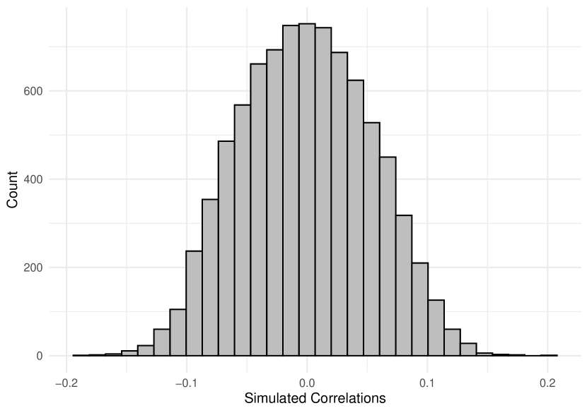
Figure 2: Histogram of the simulated correlations $\rho_{ijk}$ in LP’s simulation study, where $X_{3ijk}$ was generated from $N_{3}(0,\text{CS}(0.3))$ and $\gamma$ was set to $(0.1,-0.2,0.15)^{\top}$.

There are certain specific scenarios where $E_{n}/n\to 0$, in which case, the variance estimator from Luo and Pan (2022) would give correct result. The expectation in Equation (12) is $\rho_{ijk}=\operatorname{cor}(Y_{ij},Y_{ik})$. When this expectation averaged over all $i$, $j$, and $k$ is close to zero, $E_{n}$ would be close to zero. In the simulation setting of Luo and Pan (2022), the true values of $\rho_{ijk}$’s can be calculated by $g_{3}^{-1}(X_{3ijk}\gamma)$ from Equation (2). Figure 2 shows the histogram of these true correlation parameters where $X_{3ijk}$ was generated from $N_{3}(0,\text{CS}(0.3))$ and $\gamma$ was set to $(0.1,-0.2,0.15)^{\top}$. The distribution of $\rho_{ijk}$’s exhibits a central and symmetrical pattern around 0. This explains why the flawed variance estimator of Luo and Pan (2022) had good performance in their simulation studies. In the general case where $E_{n}/n$ does not approach zero, as illustrated in our simulation study, their variance estimate does not agree with the empirical variance.

Appendix C QIC and Quasi-likelihoods

In order to select for variance and correlation models, Luo and Pan (2022) extended the QIC criterion proposed by Pan (2001) into three model selection procedures. They also integrated the penality of the BIC, which applies a stronger penalty to free parameters and favors a more parsimonious model. Let $\hat{\beta}_{n}^{f}$, $\hat{\lambda}_{n}^{f}$, and $\hat{\gamma}_{n}^{f}$ be the full model estimates, and $\hat{\beta}_{n}^{c}$, $\hat{\lambda}_{n}^{c}$, and $\hat{\gamma}_{n}^{c}$ be the candidate model estimates. The quasi-likelihoods for the mean, scale, and correlation models are defined as

$$Q_{1}(\hat{\beta}_{n}^{c},\hat{\lambda}_{n}^{f},\hat{\gamma}_{n}^{f}) =\sum_{i=1}^{n}\sum_{j=1}^{m_{i}}\int_{y_{ij}}^{\hat{\mu}_{ij}}\frac{y_{ij}-t}{\tilde{\phi}_{ij}v(t)}\,\differential t,\quad \hat{\mu}_{ij}=g_{1}^{-1}(X_{1ij}^{\top}\hat{\beta}_{n}^{c}),$$

$$Q_{2}(\hat{\beta}_{n}^{f},\hat{\lambda}_{n}^{c},\hat{\gamma}_{n}^{f}) =\sum_{i=1}^{n}\sum_{j=1}^{m_{i}}\int_{\tilde{s}_{ij}}^{\hat{\phi}_{ij}}\frac{\tilde{s}_{ij}-t}{2t^{2}}\,\differential t,\quad \hat{\phi}_{ij}=g_{2}^{-1}(X_{2ij}^{\top}\hat{\lambda}_{n}^{c}),$$

$$Q_{3}(\hat{\beta}_{n}^{f},\hat{\lambda}_{n}^{f},\hat{\gamma}_{n}^{c}) =\sum_{i=1}^{n}\sum_{j=1}^{m_{i}-1}\sum_{k=j+1}^{m_{i}}\int_{\tilde{z}_{ijk}}^{\hat{\rho}_{ijk}}\frac{\tilde{z}_{ijk}-t}{1+t^{2}}\,\differential t,\quad \hat{\rho}_{ijk}=g_{3}^{-1}(X_{3ijk}^{\top}\hat{\gamma}_{n}^{c}),$$

with $\tilde{\phi}_{ij}$, $\tilde{s}_{ij}$, and $\tilde{z}_{ijk}$ being evaluated at $\hat{\beta}_{n}^{f}$, $\hat{\lambda}_{n}^{f}$, and $\hat{\gamma}_{n}^{f}$. Subsequently, their model selection criteria are formulated as

$$\text{QIC}(\hat{\beta}_{n}^{c}) =-2Q_{1}(\hat{\beta}_{n}^{c},\hat{\lambda}_{n}^{f},\hat{\gamma}_{n}^{f})+\log(n)\text{tr}(\hat{\Omega}_{\beta n}^{c}\hat{V}_{\beta n}^{c}),\quad\hat{\Omega}_{\beta n}^{c}=\frac{-\partial^{2}Q_{1}(\beta,\hat{\lambda}_{n}^{f},\hat{\gamma}_{n}^{f})}{\partial\beta\beta^{\top}}\Biggr{\rvert}_{\beta=\hat{\beta}_{n}^{c}},$$

$$\text{QIC}(\hat{\lambda}_{n}^{c}) =-2Q_{2}(\hat{\beta}_{n}^{f},\hat{\lambda}_{n}^{c},\hat{\gamma}_{n}^{f})+\log(n)\text{tr}(\hat{\Omega}_{\lambda n}^{c}\hat{V}_{\lambda n}^{c}),\quad\hat{\Omega}_{\lambda n}^{c}=\frac{-\partial^{2}Q_{2}(\hat{\beta}_{n}^{f},\lambda,\hat{\gamma}_{n}^{f})}{\partial\lambda\lambda^{\top}}\Biggr{\rvert}_{\lambda=\hat{\lambda}_{n}^{c}},$$

$$\text{QIC}(\hat{\gamma}_{n}^{c}) =-2Q_{3}(\hat{\beta}_{n}^{f},\hat{\lambda}_{n}^{f},\hat{\gamma}_{n}^{c})+\log(n)\text{tr}(\hat{\Omega}_{\gamma n}^{c}\hat{V}_{\gamma n}^{c}),\quad\hat{\Omega}_{\gamma n}^{c}=\frac{-\partial^{2}Q_{3}(\hat{\beta}_{n}^{f},\hat{\lambda}_{n}^{f},\gamma)}{\partial\gamma\gamma^{\top}}\Biggr{\rvert}_{\gamma=\hat{\gamma}_{n}^{c}},$$

and $\hat{V}_{\beta n}^{c}$, $\hat{V}_{\lambda n}^{c}$, and $\hat{V}_{\lambda n}^{c}$ can be estimated by the corresponding parts of the sandwich variance estimator.

The model selection process was carried out separately for mean, variance, and correlation. This means that during the selection of the mean model, $\lambda$ and $\gamma$ were retained as the full model estimates $\hat{\lambda}_{n}^{f}$ and $\hat{\gamma}_{n}^{f}$ respectively. The candidate model with the lowest QIC was then chosen as the best mean model. Analogous procedures were followed for the selection of variance and scale models.

Appendix D Least Squares Approximation

Wang and Leng (2007) proposed a method that uses LSA as a simple approximation to the original loss function for achieving a unified and straightforward estimation of the least absolute shrinkage and selection operator (LASSO). Assume that there is a loss function $L_{n}(\theta)$ with a continuous second-order derivative with respect to $\theta$. This assumption is shown to be independent of the implementation of LSA and is only used to illustrate the idea. By a second-order Taylor expansion at $\hat{\theta}_{n}$,

$$n^{-1}L(\theta)\approx n^{-1}L_{n}(\hat{\theta}_{n})+n^{-1}\dot{L}_{n}(\hat{\theta}_{n})^{\top}(\theta-\hat{\theta}_{n})+\frac{1}{2}(\theta-\hat{\theta}_{n})^{\top}\left\{\frac{1}{n}\ddot{L}_{n}(\hat{\theta}_{n})\right\}(\theta-\hat{\theta}_{n}),$$ (13)

where $\dot{L}_{n}(\hat{\theta}_{n})$ and $\ddot{L}_{n}(\hat{\theta}_{n})$ are the first- and second-order derivatives of the loss function. Since $\hat{\theta}_{n}$ is a minimizer of $L_{n}(\hat{\theta}_{n})$, we know that $\dot{L}_{n}(\hat{\theta}_{n})=0$. Moreover, we can ignore $n^{-1}L_{n}(\hat{\theta})$ since it is a constant. Therefore, $n^{-1}L(\theta)$ can be approximated by a quadratic term

$$\frac{1}{2}(\theta-\hat{\theta}_{n})^{\top}\left\{\frac{1}{n}\ddot{L}_{n}(\hat{\theta}_{n})\right\}(\theta-\hat{\theta}_{n}).$$

In the framework of GEE1, if we assume the quasi-likelihood function $Q(\hat{\beta}_{n}^{c})$ is well-defined and $\hat{\beta}_{n}^{f}\approx\beta$, we can approximate $2Q(\hat{\beta}_{n}^{c})$ by expanding equation (13) at $\hat{\beta}_{n}^{f}$ as

$$(\hat{\beta}_{n}^{c}-\hat{\beta}_{n}^{f})^{\top}\left\{\ddot{L}_{n}(\hat{\beta}_{n}^{f})\right\}(\hat{\beta}_{n}^{c}-\hat{\beta}_{n}^{f}).$$

where $\ddot{L}_{n}(\hat{\beta}_{n}^{f})$ can be computed as the bread matrix $n\hat{\Sigma}_{1n}$ in the sandwich variance estimator because $n\hat{\Sigma}_{1n}$ is the slope matrix of the estimating equations, and the estimating equations can be viewed as the first-order slope matrix of an unknown loss function. This is different from Wang and Leng (2007), where the inverse of the estimated covariance matrix, $\hat{V}_{\hat{\beta}_{n}^{f}}^{-1}$, is used to estimate $\ddot{L}_{n}(\hat{\beta}_{n}^{f})$. In this case, assuming $Y_{ij}$ follows a normal distribution, the quadratic term reduces to the log- likelihood. Consequently, our LIC defined in equation (8) reduces to the BIC, and it reduces to the AIC if the coefficient of the penalty term is set to $2$.

References

- Carey et al. (1993) Carey, V., S. L. Zeger, and P. Diggle (1993). Modelling multivariate binary data with alternating logistic regressions. Biometrika 80(3), 517–526.
- Hin and Wang (2009) Hin, L.-Y. and Y.-G. Wang (2009). Working-correlation-structure identification in generalized estimating equations. Statistics in Medicine 28(4), 642–658.
- Højsgaard et al. (2006) Højsgaard, S., U. Halekoh, and J. Yan (2006). The R package geepack for generalized estimating equations. Journal of Statistical Software 15, 1–11.
- Kastner and Ziegler (1999) Kastner, C. and A. Ziegler (1999). A comparison of Jackknife estimators of variance for GEE2. Discussion Paper 167, Ludwig–Maximilians University of Munich, SFB 386.
- Liang and Zeger (1986) Liang, K.-Y. and S. L. Zeger (1986). Longitudinal data analysis using generalized linear models. Biometrika 73(1), 13–22.
- Luo and Pan (2022) Luo, R. and J. Pan (2022). Conditional generalized estimating equations of mean-variance-correlation for clustered data. Computational Statistics & Data Analysis 168, 107386.
- Paik (1992) Paik, M. C. (1992). Parametric variance function estimation for nonnormal repeated measurement data. Biometrics 48(1), 19–30.
- Pan (2001) Pan, W. (2001). Akaike’s information criterion in generalized estimating equations. Biometrics 57(1), 120–125.
- Pourahmadi (1999) Pourahmadi, M. (1999). Joint mean-covariance models with applications to longitudinal data: Unconstrained parameterisation. Biometrika 86(3), 677–690.
- Prentice (1988) Prentice, R. L. (1988). Correlated binary regression with covariates specific to each binary observation. Biometrics 44(4), 1033–1048.
- Prentice and Zhao (1991) Prentice, R. L. and L. P. Zhao (1991). Estimating equations for parameters in means and covariances of multivariate discrete and continuous responses. Biometrics 47(3), 825–839.
- Smyth (1989) Smyth, G. K. (1989). Generalized linear models with varying dispersion. Journal of the Royal Statistical Society: Series B (Methodological) 51(1), 47–60.
- Song et al. (2019) Song, W.-L., Y.-H. Zhao, S.-J. Shi, G.-Y. Liu, Xian-Ying Eand Zheng, C. Morosky, Y. Jiao, and X.-J. Wang (2019). First trimester Doppler velocimetry of the uterine artery ipsilateral to the placenta improves ability to predict early-onset preeclampsia. Medicine 98(16), e15193.
- Wang and Leng (2007) Wang, H. and C. Leng (2007). Unified lasso estimation by least squares approximation. Journal of the American Statistical Association 102(479), 1039–1048.
- Wang and Carey (2003) Wang, Y.-G. and V. Carey (2003). Working correlation structure misspecification, estimation and covariate design: Implications for generalised estimating equations performance. Biometrika 90(1), 29–41.
- Wang and Lin (2005) Wang, Y.-G. and X. Lin (2005). Effects of variance-function misspecification in analysis of longitudinal data. Biometrics 61(2), 413–421.
- Yan and Fine (2004) Yan, J. and J. Fine (2004). Estimating equations for association structures. Statistics in Medicine 23(6), 859–874.
- Zhang et al. (2015) Zhang, W., C. Leng, and C. Y. Tang (2015). A joint modelling approach for longitudinal studies. Journal of the Royal Statistical Society: Series B (Statistical Methodology) 77(1), 219–238.
- Ziegler et al. (1998) Ziegler, A., C. Kastner, and M. Blettner (1998). The generalised estimating equations: An annotated bibliography. Biometrical Journal: Journal of Mathematical Methods in Biosciences 40(2), 115–139.