Deep Linear Array Pushbroom Image Restoration: A Degradation Pipeline and Jitter-Aware Restoration Network
Abstract
Linear Array Pushbroom (LAP) imaging technology is widely used in the realm of remote sensing. However, images acquired through LAP always suffer from distortion and blur because of camera jitter. Traditional methods for restoring LAP images, such as algorithms estimating the point spread function (PSF), exhibit limited performance. To tackle this issue, we propose a Jitter-Aware Restoration Network (JARNet), to remove the distortion and blur in two stages. In the first stage, we formulate an Optical Flow Correction (OFC) block to refine the optical flow of the degraded LAP images, resulting in pre-corrected images where most of the distortions are alleviated. In the second stage, for further enhancement of the pre-corrected images, we integrate two jitter-aware techniques within the Spatial and Frequency Residual (SFRes) block: 1) introducing Coordinate Attention (CoA) to the SFRes block in order to capture the jitter state in orthogonal direction; 2) manipulating image features in both spatial and frequency domains to leverage local and global priors. Additionally, we develop a data synthesis pipeline, which applies Continue Dynamic Shooting Model (CDSM) to simulate realistic degradation in LAP images. Both the proposed JARNet and LAP image synthesis pipeline establish a foundation for addressing this intricate challenge. Extensive experiments demonstrate that the proposed two-stage method outperforms state-of-the-art image restoration models. Code is available at https://github.com/JHW2000/JARNet.
Introduction
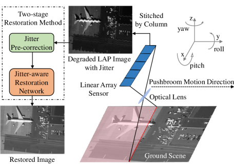
Linear array cameras are widely employed in remote sensing for high-resolution optical imaging on the earth (Cui et al. 2023; Wang, Zhu, and Fan 2018). As shown in Fig. 1, a linear array camera contains an array of sensors arranged in a straight line. The linear array sensor captures images at ground scene while the whole camera moves along the pushbroom motion direction. This movement is similar to how a broom sweeps forward. Pixels imaged at different moments are stitched together to generate a LAP image. Due to adjustments in camera attitude and periodic movement (Iwasaki 2011), inevitable jitter arises in LAP imaging. This leads to pixel displacements of varying magnitudes, thereby inducing distortion and blur within LAP images. Low-frequency jitter causes image distortion effect, while high-frequency jitter leads to blur effect (Pan et al. 2020). In practice, roll jitter causes pixel offset in the cross-track direction, and pitch jitter causes pixel offset in the along-track direction. Jitter offsets in the along-track direction are much smaller than that in the cross-track direction, while jitter in the yaw direction is tiny enough to be neglected (Wang et al. 2017).
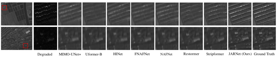
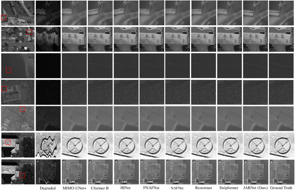
Many efforts have been made to remove distortion and blur in LAP images. Their efforts are directed towards acquiring more precise jitter curves, either directly measuring from high-resolution equipment (Pan et al. 2020) or indirectly predicting from degraded images (Wang et al. 2021). However, the former is often hindered by the scarcity of high-precision equipment, while the latter often falls short in terms of predicting accuracy. Over the years, deep learning has demonstrated outstanding performance in many image restoration tasks due to its powerful data modeling and generation capabilities. However, mainstream image restoration methods (Cho et al. 2021; Chen et al. 2021; Zamir et al. 2022; Wang et al. 2022) are not well-adopted in LAP image reconstruction due to the lack of jitter priors. As shown in Fig. 6, we test seven mainstream methods and they struggle to restore sufficient details of farmland and city buildings, showing their limitation in LAP image restoration task.
Another obstacle is the availability of data that comes with distortion and blur by jitter. As far as we are concerned, there is no customized LAP image dataset. Many studies (Zhang, Iwasaki, and Xu 2019; Wang et al. 2021) use several sinusoidal components to simulate jitter effect in LAP image (Wulich and Kopeika 1987). However, jitter in the real world is more complicated. So how to establish an efficient data synthesis pipeline remains a problem.
In this paper, we tackle the challenge of limited data availability for LAP images and propose a novel restoration pipeline for LAP image recovery. Inspired by Continue Dynamic Shooting Model (CDSM) which provides a finer-grained sampling strategy (Pan et al. 2020), we propose a novel LAP image degradation pipeline on CDSM-based jitter model, which simulates distortion and blur. We generate sufficient degraded LAP images from public dataset DOTA-v1.0 (Xia et al. 2018) for building our LAP dataset.
In order to utilize jitter prior and achieve better restoration performance, we propose JARNet, a jitter-aware restoration network based on the two-stage restoration strategy. In the first stage, we design an Optical Flow Correction (OFC) block to refine optical flow from jitter prior. Then we warp the degraded LAP image by the refined optical flow to make precise pre-correction, which removes most of the distortion. In the second stage, we design a Spatial and Frequency Residual (SFRes) block, which integrates two jitter-aware techniques of coordinate attention (Hou, Zhou, and Feng 2021) (CoA) block and frequency branch (Mao et al. 2023). The CoA block in spatial branch captures jitter state in orthogonal direction. The frequency branch parallel to the spatial branch extracts both low and high-frequency jitter, guiding the overall removal of distortion and blur. Compared with state-of-the-art methods, our proposed JARNet achieves competitive performance in LAP image restoration task. In summary, our contributions are outlined as follows:
-
•
We develop a novel LAP image synthesis pipeline with CDSM integration, which achieves a finer-grained level of simulation fidelity and boosts restoration performance.
-
•
We propose the first jitter-aware restoration network, employing optical flow correction and two jitter-aware techniques to utilize both spatial and frequency information.
-
•
Extensive experiments show that our method achieves superior results (+ 1.28dB in PSNR) compared with state-of-the-art methods on our LAP dataset.
Related Work
LAP Image Restoration for Remote Sensing
Many efforts have been made to remove distortion and blur effects in LAP images. For distortion caused by low-frequency jitter, many researchers improve the accuracy of jitter detection for image resampling. While high-precision attitude sensors (Tang et al. 2014) directly measure the attitude of linear array cameras, the feasibility is constrained by its economic viability. Some works focus on leveraging parallax imaging systems across distinct spectral bands within multispectral images for indirect prediction of jitter state (Hu, Zhang, and Liu 2018). Nevertheless, such strategies are often rendered inapplicable within the context of panchromatic LAP images. Furthermore, solutions based on deep learning have also been explored to predict jitter curves (Zhang, Iwasaki, and Xu 2019). However, these approaches only work within a limited range of jitter amplitude.
For blur effects caused by high-frequency jitter, traditional techniques are divided into blind and non-blind restoration methods. The former targets scenarios where blur kernel remains unknown, while the latter undertakes algorithms based on the point spread function (PSF) (Vimal 2019; Chen et al. 2013). Most studies usually apply the same PSF to the entire image, because jitter is regarded as uniform within a short imaging interval (Pan et al. 2020). However, this assumption is invalid for high-frequency jitter.
As the real LAP image data is rare, researchers often (Zhang, Iwasaki, and Xu 2019; Wang et al. 2021) simulate jitter effects by using multiple sinusoidal components (Wulich and Kopeika 1987). However, jitter in the real world is more intricate. Consequently, establishing an effective data synthesis pipeline remains a challenge. In this paper, we establish a CDSM-based LAP image degradation pipeline to acquire sufficient LAP data. We utilize deep learning technology and propose JARNet, to process distortion and blur in a two-stage restoration manner. We remove most of the distortions with jitter prior processed by CDSM in the first stage. Then we deal with the rest of distortion and blur effect by restoration network in the second stage.
Learning-based Single Image Restoration
Deep learning has emerged as a powerful tool for learning data-driven models end-to-end, especially in low-level vision tasks (e.g. image restoration). Many methods have achieved remarkable performance on public degraded datasets (Nah, Hyun Kim, and Mu Lee 2017; Abdelhamed, Lin, and Brown 2018; Li et al. 2023), proving their potential in natural image restoration. These methods often employ multi-scale architectures. For example, MIMO-UNet (Cho et al. 2021) utilizes multi-scale inputs and outputs, HINet (Chen et al. 2021) applies a two-stage UNet, and NAFNet (Chen et al. 2022) leverages a simplified UNet backbone. Some transformer-based approaches utilize self-attention mechanism and reduce time complexity of vanilla vision transformer (Dosovitskiy et al. 2021), such as Uformer (Wang et al. 2022), Restormer (Zamir et al. 2022) and Stripformer (Tsai et al. 2022). However, such mainstream image restoration methods do not work well in LAP image restoration task due to the domain gap between LAP and natural imaging scenes. With the refined optical flow from OFC block and two jitter-aware techniques of CoA block and frequency branch, our JARNet can capture jitter state in orthogonal direction and extract jitter at different frequencies, which is well-adopt in LAP image restoration.
Proposed Method
We first introduce the principle of LAP jitter with the CDSM-based dense sampling strategy. On this basis, we propose an image synthesis pipeline for LAP image degradation. Finally, we present the jitter-aware image restoration network, JARNet, in a two-stage restoration manner.
CDSM-Based Jitter Model
For linear array sensors in the remote sensing field, the main factor of degradation is the image deformation and blur effect caused by the camera jitter. The jitter can be described by a series of time-varying sinusoidal functions (Wulich and Kopeika 1987) in Eq. 1:
| (1) |
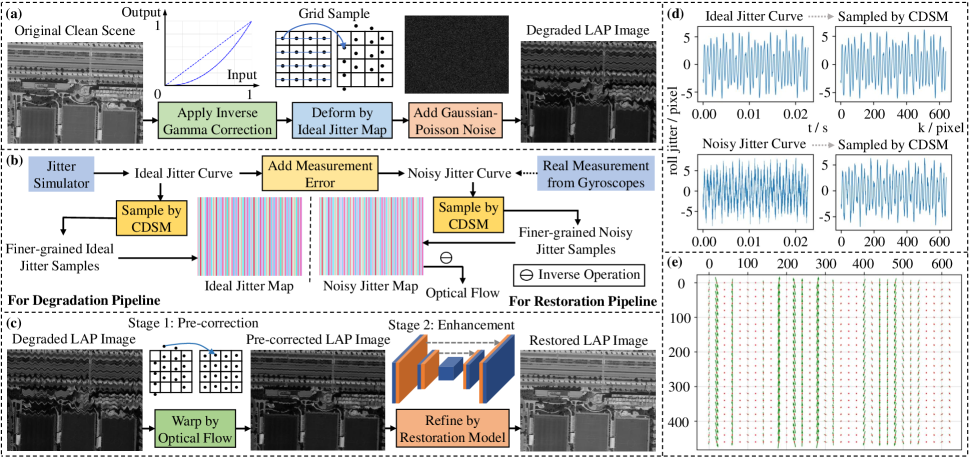
where is a time-varying jitter angle curve in a certain direction, , and are jitter amplitude, jitter frequency, and initial random phase, respectively. means the number of sinusoidal components. Due to tiny , the pixel offset on the sensor caused by jitter can be approximated by , where is the number of pixel offset in a certain direction, is focal length of optical system, and is pixel size of linear array sensor. Proportional to , consists of various sinusoidal components. As shown in Fig. 2 (b), (d), we obtain ideal jitter curve for LAP image degradation pipeline by jitter simulator in Eq. 1. The real jitter curve measured by gyroscopes is noisy that contains much measurement error. We denote it as noisy jitter curve. However, it is difficult to obtain sufficient noisy jitter curves in the real world. Therefore, we simulate noisy jitter curve for LAP two-stage restoration pipeline by adding measurement error to the ideal jitter curve.
It is worth noting that ideal jitter curve from jitter simulator simulates image distortion with only tiny blur effect. And correcting deformed LAP image directly by noisy jitter curve is imprecise. So we introduce CDSM into our jitter model to address these issues, which will be discussed in Section LAP Image Degradation Pipeline and Section Jitter-Aware Restoration Network. CDSM provides a denser sampling strategy (Pan et al. 2020). Without CDSM, we sample jitter curve at the time interval of imaging . In other words, in Eq. 1, , where is column pixel index in LAP image. With the application of CDSM, we utilize a shorter time interval for finer-grained sampling. Derived from Eq. 1, The CDSM-based jitter model is depicted by Eq. 2:
| (2) |
where is the subdivision jitter curve, , is subdivision number, is subdivision index, is time interval of imaging. With CDSM, the sample time interval becomes , achieving finer-grained sampling. In the upper right and lower right of Fig. 2 (d), we visualize the effect of CDSM by averaging finer-grained jitter curves in Eq. 3:
| (3) |
where is jitter curve processed by CDSM. Compared to their original state, the ideal jitter curve shows only minor changes, while the noisy jitter curve is smoothed.
LAP Image Degradation Pipeline
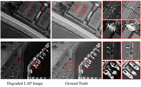
Fig. 2 (a) illustrates the pipeline of generating degraded LAP images from original clean scene. Firstly, we apply inverse gamma correction for original clean image to obtain the energy representation of the scene, as the sensor noise follows Gaussian-Poisson distribution in this domain. Next, we deform the image by ideal jitter map. Finally, Gaussian-Poisson noise is added to the deformed image.
Ideal jitter map determines the amount of jitter offset for each pixel in LAP image. Given a LAP image with shape of , where the width direction is the pushbroom direction, we establish a sampling time array . According to Eq. 2, we calculate a finer-grained ideal jitter sample in a certain direction from CDSM with a shape of , denoted as . The height direction represents the direction of the linear array sensor. Since all the pixels are imaged at the same time, their jitter states remain consistent. So we simply duplicate the jitter sample along the height direction to a shape of . Subsequently, we concatenate jitter from roll and pitch direction, resulting in an ideal jitter map with a shape of . Eq. 4 shows the process above.
| (4) |
where is the subdivided ideal jitter map. is duplicate operation. represents the height direction. is concatenate operation. Finally, we make a grid sample to deform LAP image by several subdivision ideal jitter maps. Since the pixel offset may not be an integer, we apply bilinear interpolation during resampling. The LAP image degradation pipeline is depicted by Eq. 5:
| (5) |
where is the degraded LAP image, is the original image, is inverse gamma correction coefficient, denotes grid sample operation, and is Gaussian-Poisson noise. Through averaging deformed LAP images from ideal jitter maps with different subdivision indexes, we successfully introduce blur effect into degraded LAP image thanks to CDSM-based jitter model.
Finally, we establish our LAP dataset through our proposed degradation pipeline, which contains degraded-clean LAP image pairs. We demonstrate two LAP image pairs and their zoom-in details in Fig. 3.
Jitter-Aware Restoration Network
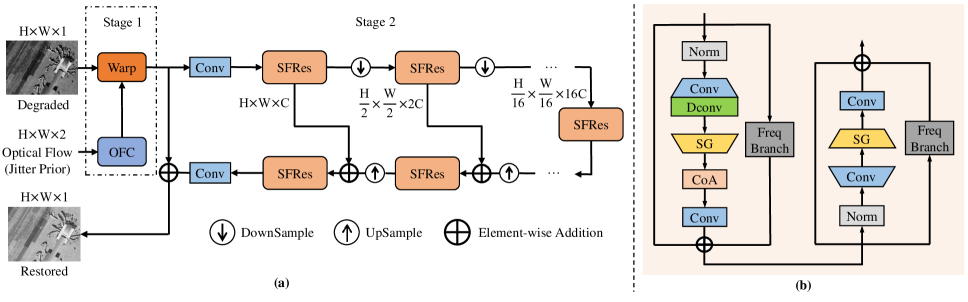
To restore the LAP images from the pixel displacement and blur caused by camera jitter, we propose a jitter-aware restoration network, JARNet, which restores LAP images in two stages, as shown in Fig. 2 (c). The first stage is called the pre-correction stage, where most of the distortion in degraded LAP image is removed by optical flow. Noticeably, we introduce Optical Flow Correction (OFC) block in JARNet to enable more precise warping and effective distortion removal. The second stage is called the enhancement stage, where we employ a Spatial and Frequency Residual (SFRes) block in the U-shaped network to further enhance the pre-corrected LAP image. The two-stage restoration strategy offers us an effective approach to enhance the performance of state-of-the-art methods in LAP image restoration task. We will introduce the two stages, the proposed jitter-aware techniques, and losses in the following paragraphs.
Pre-correction Stage and OFC Block Since jitter state provides degradation information, we attempt to use it as prior to warp the distorted LAP images in the pre-correction stage. Specifically, we simulate several subdivided noisy jitter maps from noisy jitter curve as shown in Fig. 2 (b), whose process is similar to ideal jitter map. Then we average all the subdivided noisy jitter maps, assisting in smoothing the noise thanks to CDSM-based jitter model. Subsequently, the degraded LAP image is warped by optical flow in Eq. 6, which is approximated as the inverse of noisy jitter map:
| (6) |
where is the pre-corrected image, most of whose distortions are removed. denotes optical flow, and denotes noisy jitter map. Fig. 2 (e) shows the optical flow map with shape of . The vector at each pixel represents direction and relative magnitude of pixel offset.
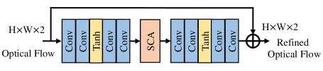
Instead of warping the degraded image by original optical flow, we refine the optical flow by our proposed Optical Flow Correction (OFC) block. As shown in Fig. 5, the OFC block has a shallow attention-based convolution architecture and employs the SCA module (Chen et al. 2022) to reweight feature map of optical flow between roll and pitch directions, which assists better embedding of jitter prior. Then we utilize the refined optical flow to warp the degraded image.
Enhancement Stage and SFRes Block Since optical flow is calculated approximately, there still remains little distortion and blur in pre-corrected LAP image. In the enhancement stage, we further improve the LAP image quality by a U-shaped network with Spatial and Frequency Residual (SFRes) blocks as key blocks, as illustrated in Eq. 7:
| (7) |
where is restored image. is restoration network. is parameter set in image restoration network. As shown in Fig. 4, the enhancement stage adopts a U-shaped network with skip connections between the encoder and the decoder. After the initial convolution layer, each level of encoder and decoder uses a series of SFRes blocks, inspired by the design of NAFNet block (Chen et al. 2022). The SFRes block includes a spatial branch, a frequency branch, and a residual path, taking advantage of both local and global information. In both of the two kinds of branches, we adopt jitter-aware techniques to further improve the LAP image quality.
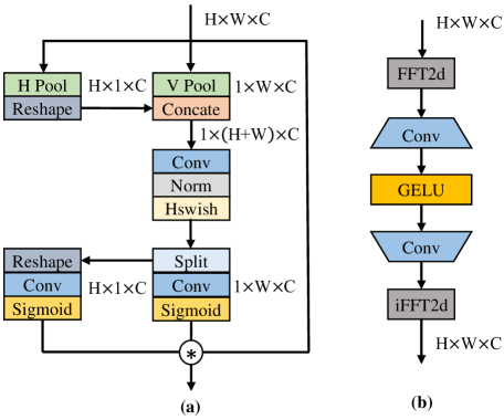
The spatial branch of SFRes block employs coordinate attention (CoA) (Hou, Zhou, and Feng 2021) block to reweight feature map in the vertical and horizontal directions of LAP image. With the input feature shape of , CoA outputs two attention maps with shapes of and , respectively. Then element-wise multiplication is applied between the input feature map and attention maps. CoA block helps capture the jitter state in orthogonal directions for better LAP image restoration.
The frequency branch (Mao et al. 2023) in the SFRes applies fast Fourier transform algorithm to convert the feature map to the frequency domain. Each pixel of feature map in frequency branch contains global information of LAP image, which not only extracts both low and high-frequency jitter but also assists in restoring high-frequency details.
Losses To supervise the training of JARNet, we apply a restoration loss and an optical flow loss in the total loss function , as illustrated in Eq. 8:
| (8) |
where . The refined optical flow is supervised by noise-free optical flow , where . We define the flow loss in Eq. 9:
| (9) |
where is mean absolute error loss function. is utilized to constrain the optimization of the optical flow. We train OFC block as part of JARNet in a joint end-to-end manner. We apply a restoration loss to supervise the training of JARNet between and in Eq. 10:
| (10) |
where and . contains 3 components, mean absolute error loss, perceptual loss (Johnson, Alahi, and Li 2016), and FFT loss (Cho et al. 2021).
Experiments
Dataset
We utilize DOTA-v1.0 dataset (Xia et al. 2018) as our source of clean data, which is originally designed for object detection in aerial images. We apply our proposed LAP image degradation pipeline on training set of DOTA-v1.0, which contains 2,806 images, to create our simulated LAP dataset. We crop each image into a size of . For degradation parameter, in Hz, in pixel number, (Teshima and Iwasaki 2007; Zhu et al. 2018), , . We simulate four main sinusoidal components. To promise a larger degradation space, for each cropped image we multiply amplitude and frequency respectively by a vibration factor, where amplitude vibration factor satisfies Gaussian distribution with , and frequency vibration factor satisfies Gaussian distribution with , . The Gaussian-Poisson noise is applied with , . The maximum jitter measurement error is 20% of current jitter offset. Overall, we obtain 20,614 train image pairs and 2,577 test image pairs in our synthetic LAP dataset.
Implementation Details
Our experiments are all trained and evaluated on our LAP image dataset. We set our batch size as 4 and training patch size as . We train our JARNet from scratch for 450k steps on a single NVIDIA GeForce RTX 4090 GPU with 24GB of memory, which takes approximately 26 hours. We apply AdamW (Loshchilov and Hutter 2019) optimizer (, , weight decay ). Cosine learning rate strategy is applied from to . We compare our proposed method with other state-of-the-art approaches on our LAP image dataset. For a fair comparison, other methods are all trained from scratch on our LAP dataset. Except for batch size, patch size, and training steps, we follow the training protocols of each method if not specified. In testing, we use PSNR, SSIM, and gradient magnitude similarity deviation (GMSD) (Xue et al. 2013) as our evaluation metrics with the full image size of .
Comparisons with State-of-the-Art Methods
| Models | PSNR(dB) | SSIM | GMSD | Params(M) |
|---|---|---|---|---|
| MIMO-UNet+ | 34.94 | 0.9127 | 0.0447 | 16.10 |
| Uformer-B | 36.08 | 0.9213 | 0.0439 | 50.88 |
| HINet | 36.18 | 0.9208 | 0.0376 | 88.66 |
| FNAFNet | 36.94 | 0.9311 | 0.0370 | 68.02 |
| NAFNet | 36.95 | 0.9291 | 0.0366 | 67.89 |
| Restormer | 37.51 | 0.9366 | 0.0344 | 26.12 |
| Stripformer | 37.74 | 0.9389 | 0.0326 | 19.71 |
| MST-L | 35.67 | 0.9155 | 0.0464 | 2.03 |
| MST++ | 35.65 | 0.9154 | 0.0456 | 1.33 |
| CST-L∗ | 35.16 | 0.9083 | 0.0499 | 3.00 |
| DAUHST-9stg | 36.08 | 0.9214 | 0.0435 | 6.15 |
| HDNet | 34.43 | 0.8958 | 0.0595 | 2.37 |
| JARNet(Ours) | 39.02 | 0.9493 | 0.0239 | 13.46 |
We compare the proposed method on our LAP dataset with the following RGB-based methods: MIMO-UNet+ (Cho et al. 2021), HINet (Chen et al. 2021), Uformer-B (Wang et al. 2022), NAFNet (Chen et al. 2022), Restormer (Zamir et al. 2022), Stripformer (Tsai et al. 2022), and FNAFNet (Mao et al. 2023). Some spectral-based methods, such as MST (Cai et al. 2022b), MST++ (Cai et al. 2022c), CST (Cai et al. 2022a), DAUHST (Cai et al. 2022d), and HDNet (Hu et al. 2022), are also evaluated. Quantitative evaluation results in Tab. 1 demonstrate that our proposed JARNet outperforms all other state-of-the-art methods in terms of PSNR, SSIM, and GMSD. Compared to the existing best single image restoration method, JARNet achieves 39.02dB in PSNR and 0.9493 in SSIM, which corresponds to 1.28dB improvement in PSNR, 0.0104 improvements in SSIM and 0.0087 improvements in GMSD. Fig. 6 presents visual comparison of an interior details of farmland and city buildings. Our proposed JARNet not only effectively removes jitter in LAP images but also successfully recovers more details in the contour of farmland and buildings. While other existing methods can effectively remove deformation caused by jitter, most of them fail to remove blur effect and recover sufficient details. In contrast, JARNet utilizes the prior knowledge of jitter to make pre-correction in the first stage and reduces the learning difficulty for subsequent restoration network so as to pay more attention to image details.
Ablation Studies
Effectiveness of Pre-Correction
| Models | PSNR(dB) | SSIM | GMSD | GMACs |
|---|---|---|---|---|
| MIMO-UNet+∗ | 36.07 | 0.9402 | 0.0293 | 154.3 |
| Uformer-B∗ | 37.93 | 0.9431 | 0.0286 | 85.75 |
| HINet∗ | 37.97 | 0.9425 | 0.0275 | 170.3 |
| FNAFNet∗ | 37.70 | 0.9404 | 0.0296 | 63.34 |
| NAFNet∗ | 38.01 | 0.9428 | 0.0279 | 63.18 |
| Restormer∗ | 38.46 | 0.9472 | 0.0263 | 140.8 |
| Stripformer∗ | 38.72 | 0.9500 | 0.0247 | 170.4 |
| JARNet(Ours) | 39.02 | 0.9493 | 0.0239 | 85.71 |
To validate the effectiveness of pre-correction, we utilize jitter prior to enhance other methods in a two-stage restoration manner as shown in Fig. 2 (c). Tab. 2 shows that performances of all methods enhanced by jitter prior are improved, compared with Tab. 1. Notably, Stripformer∗ achieves a slightly higher SSIM compared with our method, while JARNet maintains the best PSNR, GMSD metric, and relatively acceptable amount of GMACs among all methods. The pre-correction in the first stage effectively reduces learning difficulty of restoration network in the second stage, leading to enhanced performance for mainstream methods.
| No. | Freq | CoA | OFC | PSNR | SSIM | Params(M) |
|---|---|---|---|---|---|---|
| 1 | 38.17 | 0.9444 | 13.80 | |||
| 2 | 37.98 | 0.9428 | 13.94 | |||
| 3 | 38.50 | 0.9478 | 12.26 | |||
| 4 | 38.56 | 0.9463 | 14.87 | |||
| 5 | 38.69 | 0.9492 | 12.39 | |||
| 6 | 38.44 | 0.9456 | 15.01 | |||
| 7 | 38.69 | 0.9471 | 13.33 | |||
| 8(Ours) | 39.02 | 0.9493 | 13.46 |
Effectiveness of Components in JARNet
In this section, we verify the effectiveness of frequency branch, CoA block, and OFC block in JARNet by conducting 7 extra experiments. As shown in Tab. 3, when we add CoA block alone in No.3, we observe a significant performance gain of 0.33dB in PSNR compared with No.1 baseline. This improvement indicates that the CoA block is effective in extracting orthogonal jitter state. Additionally, the number of parameters reduces by 11.2% approximately, indicating the efficiency of incorporating the CoA block in our JARNet. When we add frequency branch in No.2, the performance has a decline of 0.19dB in PSNR, compared with No.1 baseline. Nevertheless, by incorporating the global information extracted by frequency branch and jitter state extracted by CoA block, No.5 achieves better performance compared with No.3. So we apply frequency branch and CoA block simultaneously. Similarly, when we add OFC block in No.4, we achieve a performance gain of 0.39dB in PSNR, compared with No.1 baseline. This improvement indicates that refined optical flow effectively pre-corrects degraded LAP image. For the best restoration performance, we apply all three components in No.8 JARNet.
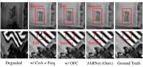
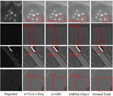
We further analyze visual results of different combinations of components. As shown in Fig. 7, when the frequency branch and CoA block are combined, the vertical details in the window are partly restored, which indicates that the CoA block, along with the frequency domain branch, has capabilities to capture jitter state and high-frequency features. OFC block helps reconstruct zebra crossing correctly on the edge of the degraded
| NAFNet∗ | Restormer∗ | Stripformer∗ | JARNet(Ours) | |
|---|---|---|---|---|
| PSNR | 36.64 | 37.06 | 37.52 | 38.50 |
| SSIM | 0.9270 | 0.9338 | 0.9403 | 0.9465 |
image. In situations where pre-corrected images have black edges, architectures without OFC block fail to handle the edge details correctly. However, the application of the OFC block helps alleviate the influence of these black edges, resulting in better restoration of edge details. Our JARNet combines advantages of all three components and achieves high-quality restoration results.
Effectiveness of CDSM
In order to verify CDSM enhances the restoration effect of the LAP dataset. We remove CDSM and generate a new CDSM-free LAP dataset on which we compare different enhanced state-of-the-art methods. As shown in Tab. 4, other enhanced methods suffer from a sharp performance decline compared with results in Tab. 2, even worse than non-enhanced versions in Tab. 1. Without CDSM, the noisy jitter curve is not smoothed. Therefore, pre-correction in the first stage does not work. However, JARNet only shows a slight decrease in performance, because the OFC block in the first stage compensates part of smoothing effect from CDSM. This fully demonstrates the importance of CDSM in LAP image restoration pipeline. CDSM helps smooth the noisy jitter curve and obtain better pre-correction results.
Conclusion
In order to restore degraded LAP image caused by camera jitter and overcome the obstacle of data availability, we proposed a CDSM-based LAP image degradation pipeline and created a LAP dataset. Then we presented the first jitter-aware restoration network in a two-stage restoration manner. In the first stage, we utilized optical flow refined by OFC block to warp the degraded LAP image. In the second stage, we incorporated CoA block and frequency branch in SFRes block to realize jitter-aware character. CoA block captures jitter state in orthogonal direction, while frequency branch extracts both low and high-frequency jitter. Extensive experiments demonstrate that our approach performs favorably against state-of-the-art methods qualitatively and quantitatively on our LAP dataset.
Acknowledgments
This project is supported by National Natural Science Foundation of China (No. 62275229). We thank Meijuan Bian and Weige Lyu from the facility platform of optical engineering of Zhejiang University for instrument support.
Appendix
Approximation of Optical Flow
In this section, we discuss the reason why we make an approximation between optical flow and the inverse of jitter map. For simplicity we only consider distortion. The process of deforming a clean image is shown in Eq. 11:
| (11) |
where and represent pixel position in the image, and is a jitter map. and is pixel displacement at original position . We pre-correct the deformed image precisely in Eq. 12:
| (12) |
where and represent pixel position in the pre-corrected image. Theoretically, we need jitter data at the original position . However, we only have deformed image and measured jitter data . We do not know where the original position is. On the other hand, and are probably not integers. In practice, is processed by bilinear interpolation algorithm during the process of grid sample.
To make Eq. 12 computable, we assume the jitter data at new position is approximately equaled to that in original position , as shown in Eq. 13:
| (13) |
For height direction, the jitter state keeps the same, because the pixels along the height direction are imaged at the same time. We make an approximation in the width direction, because jitter offsets in the along-track direction are much smaller than that in the cross-track direction (Wang et al. 2017). So we treat the inverse of jitter map as optical flow for pre-correction.
More Architecture Details of JARNet
We adopt NAFNet (Chen et al. 2022) as the backbone of JARNet, with 4 levels of encoder and decoder. We set 32 as the width of JARNet, with 36 SFRes blocks in total. Each level of encoder and decoder contains 4 SFRes blocks, and the middle bottleneck also contains 4 SFRes blocks.
We demonstrate the architecture details of the CoA block and frequency branch in Fig. 8. The CoA block manipulates attention maps in both horizontal and vertical directions. Feature map with the shape of is applied element-wise multiplication respectively with two attention maps by the broadcast mechanism in Python.
It is worth noting that different levels of encoder and decoder extract information at varying levels. To control the receptive field, we employ a window partition strategy (Mao et al. 2023) in the frequency branch. This strategy is taken because shallow levels focus on extracting local degradation. On the other hand, deep levels are responsible for detecting global jitter states. In practice, we set the window size in the first level as 64, which means only a spatial region is considered when extracting frequency domain information. Window partition in other levels is disabled, allowing for feature extraction in the global context.
Real-World LAP Image Restoration Results
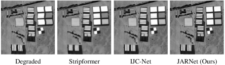
We conducted experiments on real-world LAP images from Yaogan-26 satellite (Wang et al. 2017) and show results in Fig. 9. We did the same pre-processing for degraded image before implementing Stripformer and JARNet. Compared to Stripformer and IJC-Net (Zhang, Iwasaki, and Xu 2019), JARNet achieves the best visual result, where most of the distortion and blur are removed.
More Visual Results of Restored LAP Images
Recovery Performance on More Remote Datasets
In order to validate the generalization ability of JARNet, we utilize the model trained on our original LAP dataset from DOTA-v1.0 to restore other remote datasets simulated by our degradation pipeline without finetune.
We choose AID and PatternNet as our samples. AID (Xia et al. 2017) is a large-scale aerial image dataset by collecting sample images from Google Earth imagery. AID dataset contains 10,000 images of size within 30 classes. PatternNet (Zhou et al. 2018) is a large-scale high-resolution dataset for remote sensing image retrieval. There are 38 classes and each class has 800 images of size .
We make two new LAP datasets (abbreviated as the original name of the dataset) based on AID and PatternNet through our LAP degradation pipeline, respectively. We crop images in AID into a size of , while we keep the original resolution in PatternNet. All simulated image pairs are utilized for test. We acquire 10,000 image pairs in AID and 30.400 image pairs in PatternNet.
| Models | PSNR(dB) | SSIM | PSNR(dB) | SSIM |
|---|---|---|---|---|
| NAFNet | 28.66 | 0.8798 | 30.46 | 0.8727 |
| Restormer | 32.79 | 0.9038 | 31.22 | 0.8863 |
| Stripformer | 32.92 | 0.9052 | 31.28 | 0.8869 |
| NAFNet∗ | 32.06 | 0.9048 | 31.55 | 0.8981 |
| Restormer∗ | 33.47 | 0.9204 | 32.15 | 0.9072 |
| Stripformer∗ | 33.81 | 0.9247 | 32.39 | 0.9107 |
| JARNet | 34.12 | 0.9241 | 33.40 | 0.9159 |
As shown in Tab. 5, our JARNet keeps a good performance while transferring to other datasets without finetune. Compared with other state-of-the-art methods, our JARNet keeps the performance advantage on AID and PatternNet, showing the great generalization ability of JARNet.
References
- Abdelhamed, Lin, and Brown (2018) Abdelhamed, A.; Lin, S.; and Brown, M. S. 2018. A high-quality denoising dataset for smartphone cameras. In Proceedings of the IEEE/CVF Conference on Computer Vision and Pattern Recognition (CVPR), 1692–1700.
- Cai et al. (2022a) Cai, Y.; Lin, J.; Hu, X.; Wang, H.; Yuan, X.; Zhang, Y.; Timofte, R.; and Van Gool, L. 2022a. Coarse-to-Fine Sparse Transformer for Hyperspectral Image Reconstruction. In Proceedings of the European Conference on Computer Vision (ECCV), 686–704.
- Cai et al. (2022b) Cai, Y.; Lin, J.; Hu, X.; Wang, H.; Yuan, X.; Zhang, Y.; Timofte, R.; and Van Gool, L. 2022b. Mask-Guided Spectral-Wise Transformer for Efficient Hyperspectral Image Reconstruction. In Proceedings of the IEEE/CVF Conference on Computer Vision and Pattern Recognition (CVPR), 17502–17511.
- Cai et al. (2022c) Cai, Y.; Lin, J.; Lin, Z.; Wang, H.; Zhang, Y.; Pfister, H.; Timofte, R.; and Van Gool, L. 2022c. MST++: Multi-Stage Spectral-Wise Transformer for Efficient Spectral Reconstruction. In Proceedings of the IEEE/CVF Conference on Computer Vision and Pattern Recognition (CVPR) Workshops, 745–755.
- Cai et al. (2022d) Cai, Y.; Lin, J.; Wang, H.; Yuan, X.; Ding, H.; Zhang, Y.; Timofte, R.; and Gool, L. V. 2022d. Degradation-Aware Unfolding Half-Shuffle Transformer for Spectral Compressive Imaging. In Advances in Neural Information Processing Systems (NeurIPS), volume 35, 37749–37761.
- Chen et al. (2013) Chen, H.; Cao, M.; Wang, H.; Yan, Y.; and Ma, L. 2013. Estimating the point spread function of motion-blurred images of the Ochotona Curzoniae. In 2013 6th International Congress on Image and Signal Processing (CISP), volume 1, 369–373. IEEE.
- Chen et al. (2022) Chen, L.; Chu, X.; Zhang, X.; and Sun, J. 2022. Simple baselines for image restoration. In Proceedings of the European Conference on Computer Vision (ECCV), 17–33.
- Chen et al. (2021) Chen, L.; Lu, X.; Zhang, J.; Chu, X.; and Chen, C. 2021. Hinet: Half instance normalization network for image restoration. In Proceedings of the IEEE/CVF Conference on Computer Vision and Pattern Recognition (CVPR), 182–192.
- Cho et al. (2021) Cho, S.-J.; Ji, S.-W.; Hong, J.-P.; Jung, S.-W.; and Ko, S.-J. 2021. Rethinking coarse-to-fine approach in single image deblurring. In Proceedings of the IEEE/CVF International Conference on Computer Vision (ICCV), 4641–4650.
- Cui et al. (2023) Cui, Y.; Liu, C.; Liu, S.; Xu, M.; and Xie, P. 2023. Optical design and precision analysis of a single-line-array pendulum sweep high-resolution mapping camera. Applied Optics, 62(5): 1183–1192.
- Dosovitskiy et al. (2021) Dosovitskiy, A.; Beyer, L.; Kolesnikov, A.; Weissenborn, D.; Zhai, X.; Unterthiner, T.; Dehghani, M.; Minderer, M.; Heigold, G.; Gelly, S.; Uszkoreit, J.; and Houlsby, N. 2021. An Image is Worth 16x16 Words: Transformers for Image Recognition at Scale. In International Conference on Learning Representations (ICLR).
- Hou, Zhou, and Feng (2021) Hou, Q.; Zhou, D.; and Feng, J. 2021. Coordinate attention for efficient mobile network design. In Proceedings of the IEEE/CVF Conference on Computer Vision and Pattern Recognition (CVPR), 13713–13722.
- Hu, Zhang, and Liu (2018) Hu, K.; Zhang, Y.; and Liu, W. 2018. High-frequency jitter detection by registration error curve of high-resolution multi-spectral satellite image. In 2018 26th International Conference on Geoinformatics, 1–6. IEEE.
- Hu et al. (2022) Hu, X.; Cai, Y.; Lin, J.; Wang, H.; Yuan, X.; Zhang, Y.; Timofte, R.; and Van Gool, L. 2022. HDNet: High-Resolution Dual-Domain Learning for Spectral Compressive Imaging. In Proceedings of the IEEE/CVF Conference on Computer Vision and Pattern Recognition (CVPR), 17542–17551.
- Iwasaki (2011) Iwasaki, A. 2011. Detection and estimation satellite attitude jitter using remote sensing imagery. Advances in Spacecraft Technologies, 13: 257–272.
- Johnson, Alahi, and Li (2016) Johnson, J.; Alahi, A.; and Li, F.-F. 2016. Perceptual losses for real-time style transfer and super-resolution. In Proceedings of the European Conference on Computer Vision (ECCV), 694–711.
- Li et al. (2023) Li, H.; Zhang, Z.; Jiang, T.; Luo, P.; Feng, H.; and Xu, Z. 2023. Real-world deep local motion deblurring. In Proceedings of the AAAI Conference on Artificial Intelligence, volume 37, 1314–1322.
- Loshchilov and Hutter (2019) Loshchilov, I.; and Hutter, F. 2019. Decoupled Weight Decay Regularization. In International Conference on Learning Representations (ICLR).
- Mao et al. (2023) Mao, X.; Liu, Y.; Liu, F.; Li, Q.; Shen, W.; and Wang, Y. 2023. Intriguing findings of frequency selection for image deblurring. In Proceedings of the AAAI Conference on Artificial Intelligence, volume 37, 1905–1913.
- Nah, Hyun Kim, and Mu Lee (2017) Nah, S.; Hyun Kim, T.; and Mu Lee, K. 2017. Deep multi-scale convolutional neural network for dynamic scene deblurring. In Proceedings of the IEEE Conference on Computer Vision and Pattern Recognition (CVPR), 3883–3891.
- Pan et al. (2020) Pan, J.; Ye, G.; Zhu, Y.; Song, X.; Hu, F.; Zhang, C.; and Wang, M. 2020. Jitter detection and image restoration based on continue dynamic shooting model for high-resolution TDI CCD satellite images. IEEE Transactions on Geoscience and Remote Sensing, 59(6): 4915–4933.
- Ramachandran, Zoph, and Le (2018) Ramachandran, P.; Zoph, B.; and Le, Q. V. 2018. Searching for Activation Functions. In 6th International Conference on Learning Representations, ICLR 2018 Workshop Track Proceedings.
- Tang et al. (2014) Tang, X.; Xie, J.; Wang, X.; and Jiang, W. 2014. High-precision attitude post-processing and initial verification for the ZY-3 satellite. Remote Sensing, 7(1): 111–134.
- Teshima and Iwasaki (2007) Teshima, Y.; and Iwasaki, A. 2007. Correction of attitude fluctuation of Terra spacecraft using ASTER/SWIR imagery with parallax observation. IEEE Transactions on Geoscience and Remote Sensing, 46(1): 222–227.
- Tsai et al. (2022) Tsai, F.-J.; Peng, Y.-T.; Lin, Y.-Y.; Tsai, C.-C.; and Lin, C.-W. 2022. Stripformer: Strip transformer for fast image deblurring. In Proceedings of the European Conference on Computer Vision (ECCV), 146–162.
- Vimal (2019) Vimal, V. 2019. Mixture of Gaussian Blur Kernel Representation for Blind Image Restoration. Turkish Journal of Computer and Mathematics Education (TURCOMAT), 10(1): 589–595.
- Wang et al. (2017) Wang, M.; Fan, C.; Pan, J.; Jin, S.; and Chang, X. 2017. Image jitter detection and compensation using a high-frequency angular displacement method for Yaogan-26 remote sensing satellite. ISPRS Journal of Photogrammetry and Remote Sensing, 130: 32–43.
- Wang, Zhu, and Fan (2018) Wang, M.; Zhu, Y.; and Fan, C. 2018. Development of platform jitter geometric analysis and processing for high-resolution optical satellite imagery. Geomatics and Information Science of Wuhan University, 43(12): 1899–1908.
- Wang et al. (2022) Wang, Z.; Cun, X.; Bao, J.; Zhou, W.; Liu, J.; and Li, H. 2022. Uformer: A general u-shaped transformer for image restoration. In Proceedings of the IEEE/CVF Conference on Computer Vision and Pattern Recognition (CVPR), 17683–17693.
- Wang et al. (2021) Wang, Z.; Zhang, Z.; Dong, L.; and Xu, G. 2021. Jitter detection and image restoration based on generative adversarial networks in satellite images. Sensors, 21(14): 4693.
- Wulich and Kopeika (1987) Wulich, D.; and Kopeika, N. 1987. Image resolution limits resulting from mechanical vibrations. Optical engineering, 26(6): 529–533.
- Xia et al. (2018) Xia, G.-S.; Bai, X.; Ding, J.; Zhu, Z.; Belongie, S.; Luo, J.; Datcu, M.; Pelillo, M.; and Zhang, L. 2018. DOTA: A Large-Scale Dataset for Object Detection in Aerial Images. In Proceedings of the IEEE/CVF Conference on Computer Vision and Pattern Recognition (CVPR).
- Xia et al. (2017) Xia, G.-S.; Hu, J.; Hu, F.; Shi, B.; Bai, X.; Zhong, Y.; Zhang, L.; and Lu, X. 2017. AID: A benchmark data set for performance evaluation of aerial scene classification. IEEE Transactions on Geoscience and Remote Sensing, 55(7): 3965–3981.
- Xue et al. (2013) Xue, W.; Zhang, L.; Mou, X.; and Bovik, A. C. 2013. Gradient magnitude similarity deviation: A highly efficient perceptual image quality index. IEEE transactions on image processing, 23(2): 684–695.
- Zamir et al. (2022) Zamir, S. W.; Arora, A.; Khan, S.; Hayat, M.; Khan, F. S.; and Yang, M.-H. 2022. Restormer: Efficient transformer for high-resolution image restoration. In Proceedings of the IEEE/CVF Conference on Computer Vision and Pattern Recognition (CVPR), 5728–5739.
- Zhang, Iwasaki, and Xu (2019) Zhang, Z.; Iwasaki, A.; and Xu, G. 2019. Attitude jitter compensation for remote sensing images using convolutional neural network. IEEE Geoscience and Remote Sensing Letters, 16(9): 1358–1362.
- Zhou et al. (2018) Zhou, W.; Newsam, S.; Li, C.; and Shao, Z. 2018. PatternNet: A benchmark dataset for performance evaluation of remote sensing image retrieval. ISPRS journal of photogrammetry and remote sensing, 145: 197–209.
- Zhu et al. (2018) Zhu, Y.; Wang, M.; Cheng, Y.; He, L.; and Xue, L. 2018. An improved jitter detection method based on parallax observation of multispectral sensors for Gaofen-1 02/03/04 satellites. Remote Sensing, 11(1): 16.