Completely Occluded and Dense Object Instance Segmentation Using Box Prompt-Based Segmentation Foundation Models

Abstract

Completely occluded and dense object instance segmentation (IS) is an important and challenging task. Although current amodal IS methods can predict invisible regions of occluded objects, they are difficult to directly predict completely occluded objects. For dense object IS, existing box-based methods are overly dependent on the performance of bounding box detection. In this paper, we propose CFNet, a coarse-to-fine IS framework for completely occluded and dense objects, which is based on box prompt-based segmentation foundation models (BSMs). Specifically, CFNet first detects oriented bounding boxes (OBBs) to distinguish instances and provide coarse localization information. Then, it predicts OBB prompt-related masks for fine segmentation. To predict completely occluded object instances, CFNet performs IS on occluders and utilizes prior geometric properties, which overcomes the difficulty of directly predicting completely occluded object instances. Furthermore, based on BSMs, CFNet reduces the dependence on bounding box detection performance, improving dense object IS performance. Moreover, we propose a novel OBB prompt encoder for BSMs. To make CFNet more lightweight, we perform knowledge distillation on it and introduce a Gaussian smoothing method for teacher targets. Experimental results demonstrate that CFNet achieves the best performance on both industrial and publicly available datasets.

I INTRODUCTION

Instance segmentation (IS) provides foundational information for numerous robot vision-based tasks, such as robot grasping [1] and robot picking [2]. It involves distinguishing and delineating each distinct object of interest appearing in an image. Deep learning-based methods [3, 4] have brought great progress to IS. While current works mainly focus on IS tasks of general objects, this work mainly studies completely occluded and dense object IS. IS of completely occluded and dense objects has important applications in the field of robot vision, such as industrial robotic automatic assembly and unmanned aerial vehicle (UAV) measurement [5]. Two examples of practical tasks are detailed below.

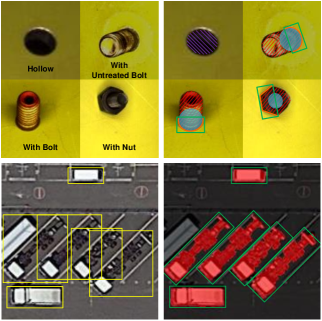
Figure 1: Examples of completely occluded and dense objects. Purple: unoccluded reference holes, yellow: horizontal bounding boxes that contain dense vehicles, green: oriented bounding boxes that contain dense vehicles or visible occluder (i.e., bolts or nuts) contours that are in the same planes as reference holes, orange: visible occluder contours that are in the same planes as reference holes, red: dense vehicles or occluders, blue: occluded reference holes.

As shown in the upper part of Fig. 1, in robotic automated assembly tasks, reference holes are responsible for providing reference positions and determining optimal assembly positions. An important task is to detect each instance of reference holes. However, in several industrial scenarios, such as aircraft assembly, reference holes (called occludees) are usually screwed with bolts and nuts, completely occluded by these industrial parts (called occluders). It is difficult to directly perform IS on occludees. An effective way is to perform IS on occluders and then use prior geometric relationships to infer occludee instances. Unlike common bounding boxes that usually encompass entire instances, in occluder IS, bounding boxes only contain parts of occluders (we refer to IS with partial bounding boxes as ISPBB). For bolts and nuts, the bounding boxes contain visible occluder contours that are in the same planes as reference holes. Then, these contour instances will be obtained from the results of ISPBB, and the occludee instances are derived from the contour instances by using prior geometric relationships. In the lower part, IS for dense objects in UAV images is a long-standing challenge. As viewed from an overhead perspective, objects are densely packed in multiple orientations. Since horizontal bounding boxes (HBBs) introduce many interference areas, oriented bounding boxes (OBBs) are often used to detect dense objects and distinguish instances.

With the development of object detection techniques, IS methods based on bounding box detection [3, 4] have gradually shown advantages, without the need for cumbersome post-processing steps. For completely occluded object IS, it requires predicting complete shapes of occludees. Many methods [6, 7, 8, 9] study amodal IS, that is, not only distinguishing the visible parts of occludees but also predicting the occluded parts. However, these methods mostly focus on IS of occludees in partially occluded scenarios. For completely occluded objects, it is very difficult to predict the occluded parts since the observable parts of occludees are too limited.

For dense object IS, since HBBs introduce many interference areas, OBBs are often used for instance identification and localization [10, 11, 12]. For example, Rotated Blend Mask R-CNN [10] performs mask prediction in OBBs. However, bounding box-based IS methods are overly dependent on the performance of object detection, especially for OBBs that are sensitive to both position and orientation. This dependence makes IS with OBBs more difficult and unstable.

In this paper, we propose a coarse-to-fine IS framework for completely occluded and dense objects, named CFNet, which is based on box prompt-based segmentation foundation models (BSMs) [13, 14]. CFNet first detects OBBs to distinguish instances, identify classes, and provide coarse localization information. Then, it predicts OBB-related segmentation masks. Our motivation is inspired by the powerful segmentation capabilities of BSMs, such as Segment Anything Model (SAM) [14], and their excellent box prompt mechanisms. CFNet uses an OBB detection module (e.g., Oriented R-CNN [15]) for coarse detection, and leverages BSMs to predict OBB-related masks for fine segmentation.

CFNet directly uses existing OBB detection methods and improves BSMs in two aspects. First, since the HBB prompt encoder is commonly used in BSMs, CFNet introduces a novel OBB prompt encoder to encode OBB prompts. Second, to make the entire model more lightweight, we perform knowledge distillation (KD) on the box prompt encoder and mask decoder. Specifically, a Gaussian label smoothing method for soft targets of the teacher model is introduced. In this work, CFNet chooses SAM as the baseline model and mainly makes improvements in the above two aspects.

Compared with amodal IS methods, CFNet provides an effective solution for completely occluded IS by performing ISPBB on occluders. In addition, OBBs used in CFNet provide more accurate location information than HBBs used in amodal IS methods. Compared with IS with OBBs, CFNet only uses OBBs as prompts to guide object segmentation, so the segmentation results are less dependent on bounding boxes, which improves IS performance. On the other hand, compared with the small-scale networks commonly used in existing IS methods, CFNet is based on BSMs that are pretrained on large-scale data for segmentation tasks. This helps CFNet enhance feature extraction and segmentation capabilities. The main contributions of this paper can be summarized as follows.

• We propose CFNet, a coarse-to-fine IS framework for completely occluded and dense objects. CFNet is based on BSMs and demonstrates the best performance on both industrial and publicly available datasets.

• A novel OBB prompt encoder is proposed to encode OBB prompts and guide BSMs to generate OBB prompt-related segmentation masks.

• We propose a KD method for the OBB prompt encoder and mask decoder of a BSM. Specifically, a Gaussian label smoothing method for soft targets generated by the teacher model is proposed.

II Related Work

II-A Amodal Instance Segmentation

Amodal IS simultaneously predicts the visible and occluded parts of occludees. The first amodal IS method [9] predicted the amodal masks and corresponding bounding boxes in an iterative bounding box expansion manner. SharpMask [16] was extended in [17] and trained on amodal IS datasets. Based on Mask R-CNN [3], Qi et al. [7] predicted occluded parts of occludees by adding a multi-task branch with multi-level coding (MLC). Similarly, based on Mask R-CNN [3], ORCNN [8] first predicted amodal masks through an amodal mask prediction branch and then combined a visible mask prediction branch to predict occluded parts. Different from the above methods that only considered occludees, BCNet [6] proposed a bilayer graph convolutional network to simultaneously consider interactions between occluders and occludees. Additionally, an amodal IS framework for building extraction is proposed in [18].

II-B Instance Segmentation with Oriented Bounding Boxes

Compared with IS with HBBs [3, 4], IS with OBBs provides more accurate location information. Based on Mask R-CNN [3], a Region of Interest (RoI) learner was applied to HBB proposals to generate OBB proposals, followed by a head that fine-tuned the OBB proposals and generated segmented masks [19]. Based on a similar idea, Feng et al. [12] proposed a part-aware IS network with OBB proposals for industrial bin picking. Follmann and König [11] first generated the final OBBs using a two-stage object detection approach, and then segmented masks within the detected OBBs. Rotated Blend Mask R-CNN [10] proposed a top-down and bottom-up structure for oriented IS.

II-C Box Prompt-Based Segmentation Foundation Models

Benefiting from pretraining on large-scale data for segmentation tasks, BSMs exhibit powerful segmentation and generalization capabilities. For example, SAM [14] was trained on more than 1B segmentation masks from 11M images, showing remarkable segmentation and zero-shot generalization capabilities. A BSM for medical image segmentation is proposed in [20]. To enhance interactive performance, BSMs incorporate prompt mechanisms, such as HBB prompts. A representative work is SAM [14], which is mainly composed of three parts: an image encoder for computing image embeddings, a prompt encoder for encoding prompts, and a lightweight mask decoder for predicting segmentation masks with respect to the prompts. MobileSAM [13] retained the prompt mechanism and proposed a lightweight version of SAM by conducting KD on SAM.

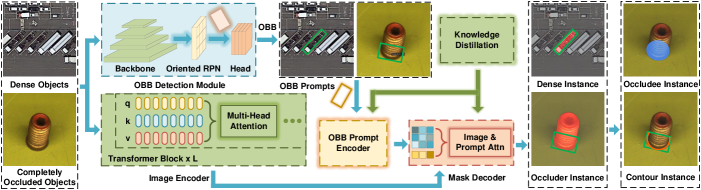
Figure 2: Architecture of the proposed CFNet. Compared with dense object IS, completely occluded object IS requires more post-processing steps to transform occluder instances into occludee instances. For clarity of presentation, only one instance is depicted in each result image of IS.

II-D Box Prompt Encoder

Existing methods usually use HBBs as box prompts for BSMs, such as SAM [14] and MobileSAM [13]. The current designs of HBB prompt encoders are mainly inspired by SAM. A HBB was represented by two points, i.e., the top-left corner point and the bottom-right corner point. Then, a point was encoded as the sum of a Gaussian positional encoding (GPE) [21] of the location (usually an embedding) and a learned embedding representing the top-left corner or bottom-right corner. Hence, a box was encoded as a combination of the two encoded point embeddings. However, there is still no encoder applicable to OBB prompts so far.

II-E Label Smoothing for Box Prompt encoders and Segmentation networks in Knowledge Distillation

In KD for segmentation tasks, label smoothing helps reduce overfitting and enhances model performance. Inception-v3 [22] proposed uniform label smoothing (ULS), i.e., the weighted average of one-hot labels and uniform distributions. Spatially varying label smoothing (SVLS) [23] applied a discrete spatial Gaussian kernel to segmentation labels to smooth one-hot labels. These two label smoothing methods were commonly used in segmentation tasks. For example, Park et al. [24] applied ULS and proposed pixel-wise adaptive label smoothing (PALS) for self-KD. P-CD [25] utilized SVLS to generate segmentation boundary uncertainty and soft targets. Unlike applying SVLS to ground truth (GT) labels, we apply Gaussian smoothing to the segmentation masks of the teacher model, which yields better distillation performance. As for label smoothing methods used for box prompt encoders, there is no relevant research published yet. We are the first to apply Gaussian label smoothing to box prompt encoders in KD.

III Methods

III-A Overview

CFNet performs ISPBB on occluders and performs IS on dense objects. The structure of CFNet is described in Fig. 2. It is mainly composed of four parts: an OBB detection module, an image encoder, an OBB prompt encoder, and a lightweight mask decoder. Specifically, images containing dense or completely occluded objects serve as input. The OBB detection module is used to detect OBBs that distinguish instances, identify classes, and provide coarse localization information. The image encoder is used to transform input images into high-dimensional feature representations and generate image embeddings. The OBB prompt encoder is responsible for encoding OBB prompts and generating prompt embeddings.

Then, the image embeddings and prompt embeddings are combined in the mask decoder to segment prompt-related masks. Especially, for completely occluded objects, post-processing needs to transform the occluder instances into contour instances. Then, by leveraging prior geometric relationships between contour instances and occludee instances, occludee instances are obtained.

Furthermore, KD is applied to the OBB prompt encoder and mask decoder to make CFNet more lightweight. For OBB detection, we employ Oriented R-CNN [15], which is a two-stage OBB detection model with competitive detection accuracy and inference speed.

III-B Oriented Bounding Box Prompt Encoder

The flowchart of the proposed OBB prompt encoder is described in Fig. 3. The detected OBBs are generated by the OBB detection module. An OBB is first parameterized as ($x_{1},y_{1},x_{2},y_{2},\sin\theta,\cos\theta$), where ($x_{1},y_{1}$), ($x_{2},y_{2}$) and ($\sin\theta,\cos\theta$) represent the top-left corner point, bottom-right corner point and orientation, respectively. We further denote

$$\bm{\varphi}_{1}=(x_{1},y_{1}),~{}~{}\bm{\varphi}_{2}=(x_{2},y_{2}),~{}~{}\bm{\theta}=(\sin\theta,\cos\theta),$$

$$\bm{\varphi}_{1}\in{[0,1)}^{2},~{}~{}\bm{\varphi}_{2}\in{[0,1)}^{2},~{}~{}\bm{\theta}\in{[0,1)}^{2},$$ (1)

where ($\bm{\varphi}_{1},\bm{\varphi}_{2}$) and $\bm{\theta}$ are normalized pixel coordinates and normalized orientation coordinates, respectively. Considering the difference between position information ($\bm{\varphi}_{1},\bm{\varphi}_{2}$) and orientation information ($\bm{\theta}$), we first encode them separately and then fuse their encoded features.

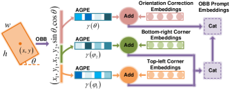
Figure 3: Architecture of the proposed OBB prompt encoder. The input is an OBB ($x,y,w,h,\theta$), where $(x,y)$, $w$, $h$ and $\theta$ represent the center point, width, height and orientation, respectively.

Coordinate-based multilayer perceptrons (MLPs) take low-dimensional coordinates as input, such as $\bm{\varphi}_{1}$, $\bm{\varphi}_{2}$ and $\bm{\theta}$, and they have difficulty learning high-frequency information [21]. In CFNet, there are many MLP structures and transformer structures containing MLPs, so such a problem will degrade IS performance. To alleviate this problem, inspired by Gaussian positional encoding (GPE) for coordinates [21], CFNet introduces adaptive GPE (AGPE) to map the coordinate set ($\bm{\varphi}_{1},\bm{\varphi}_{2},\bm{\theta}$) into random Fourier features to better learn high-frequency information and enhance the performance of coordinate-based MLPs.

Given a d-dimensional coordinate $\bm{\tau}\in{[0,1)}^{d}$, the dense Fourier feature mapping is

$$\gamma(\bm{\tau})=[ a_{0}\cos(2\pi\bm{G}_{0}^{T}\bm{\tau}),b_{0}\sin(2\pi\bm{G}_{0}^{T}\bm{\tau}),\ldots$$

$$a_{i}\cos(2\pi\bm{G}_{i}^{T}\bm{\tau}),b_{i}\sin(2\pi\bm{G}_{i}^{T}\bm{\tau}),\ldots]^{T},$$ (2)

where $a_{i}$ and $b_{i}$ ($i=0,\ldots,\infty$) are Fourier series coefficients, and $\bm{G}_{i}\in\mathbb{R}^{d}$ is the corresponding Fourier basis frequency. Since random sparse sampling of Fourier features through an MLP matches the performance of using a dense sampling of Fourier features with the same MLP [21], AGPE sets all $a_{i}$ and $b_{i}$ to 1. $\bm{G}_{i}$ is sampled from a Gaussian distribution. Hence, the mapped random Fourier features are

$$\gamma(\bm{\varphi}_{1}) =[\cos(2\pi G_{\bm{\varphi}_{1}}\bm{\varphi}_{1}),\sin(2\pi G_{\bm{\varphi}_{1}}\bm{\varphi}_{1})]^{T},$$ (3)

$$\gamma(\bm{\varphi}_{2}) =[\cos(2\pi G_{\bm{\varphi}_{2}}\bm{\varphi}_{2}),\sin(2\pi G_{\bm{\varphi}_{2}}\bm{\varphi}_{2})]^{T},$$ (4)

$$\gamma(\bm{\theta}) =[\cos(2\pi G_{\bm{\theta}}\bm{\theta}),\sin(2\pi G_{\bm{\theta}}\bm{\theta})]^{T},$$ (5)

where

$$G_{\bm{\varphi}_{1}} \in\mathbb{R}^{(l_{p},2)}\sim\mathcal{N}(\bm{\rho}{\bm{\varphi}_{1}},\bm{\Sigma}_{\bm{\varphi}_{1}}),~{}~{}\gamma(\bm{\varphi}_{1})\in\mathbb{R}^{2l_{p}},$$ (6)

$$G_{\bm{\varphi}_{2}} \in\mathbb{R}^{(l_{p},2)}\sim\mathcal{N}(\bm{\rho}{\bm{\varphi}_{2}},\bm{\Sigma}_{\bm{\varphi}_{2}}),~{}~{}\gamma(\bm{\varphi}_{2})\in\mathbb{R}^{2l_{p}},$$ (7)

$$G_{\bm{\theta}} \in\mathbb{R}^{(l_{\theta},2)}\sim\mathcal{N}(\bm{\rho}{\bm{\theta}},\bm{\Sigma}_{\bm{\theta}})~{}~{}\gamma(\bm{\theta})\in\mathbb{R}^{2l_{\theta}}.$$ (8)

The $l_{p}$ and $l_{\theta}$ are the lengths of the sampled Fourier basis frequencies. The $(\bm{\rho}{\bm{\varphi}_{1}},\bm{\rho}{\bm{\varphi}_{2}},\bm{\rho}{\bm{\theta}})$ and ($\bm{\bm{\Sigma}}_{\bm{\varphi}_{1}},\bm{\bm{\Sigma}}_{\bm{\varphi}_{2}},\bm{\bm{\Sigma}}_{\bm{\theta}}$) represent mean vectors and covariance matrices, respectively. To represent position information ($\gamma(\bm{\varphi}_{1})$, $\gamma(\bm{\varphi}_{2})$) and orientation information ($\gamma(\bm{\theta})$) in a unified representation space, we set $l_{p}=l_{\theta}$.

In many HBB prompt encoders of BSMs, $(\bm{\rho}{\bm{\varphi}_{1}},\bm{\rho}{\bm{\varphi}_{2}},\bm{\rho}{\bm{\theta}})$ and ($\bm{\bm{\Sigma}}_{\bm{\varphi}_{1}},\bm{\bm{\Sigma}}_{\bm{\varphi}_{2}},\bm{\bm{\Sigma}}_{\bm{\theta}}$) are considered as hyperparameters, which leads to difficulty in adapting to changes in datasets and searching optimal parameter settings. In CFNet, we adaptively learn ($\bm{\bm{\Sigma}}_{\bm{\varphi}_{1}},\bm{\bm{\Sigma}}_{\bm{\varphi}_{2}},\bm{\bm{\Sigma}}_{\bm{\theta}}$). $(\bm{\rho}{\bm{\varphi}_{1}},\bm{\rho}{\bm{\varphi}_{2}},\bm{\rho}{\bm{\theta}})$ are fixedly set to 0. Concretely, ($\bm{\bm{\Sigma}}_{\bm{\varphi}_{1}},\bm{\bm{\Sigma}}_{\bm{\varphi}_{2}},\bm{\bm{\Sigma}}_{\bm{\theta}}$) are the weights of a learnable embedding layer.

Inspired by SAM, the mapped random Fourier features ($\gamma(\bm{\varphi}_{1})$ and $\gamma(\bm{\varphi}_{2})$) are summed with two learned embeddings ($\bm{\omega}_{1}$ and $\bm{\omega}_{2}$) that represent the top-left corner point and bottom-right corner point in CFNet, respectively.

$$\mathcal{E}(\bm{\varphi}_{1})=\gamma(\bm{\varphi}_{1})+\bm{\omega}_{1},$$ (9)

$$\mathcal{E}(\bm{\varphi}_{2})=\gamma(\bm{\varphi}_{2})+\bm{\omega}_{2}.$$ (10)

Then, we obtain the encoded feature embeddings $\mathcal{E}(\bm{\varphi}_{p})$ with respect to position information, which is given as

$$\mathcal{E}(\bm{\varphi}_{p})=\mathrm{Concat}[\mathcal{E}(\bm{\varphi}_{1}),~{}~{}\mathcal{E}(\bm{\varphi}_{2})].$$ (11)

On the other hand, the parameterized orientation representation ($\sin\theta,\cos\theta$) of an OBB suffers from the boundary discontinuity problem [26]. Due to the periodicity of orientations, at boundary orientations (such as $0^{\circ}$ and $180^{\circ}$), small changes in orientations will result in large jumps in ($\sin\theta,\cos\theta$). To alleviate the boundary discontinuity problem, CFNet introduces learnable orientation correction embeddings $\bm{\omega}_{\theta}$. At the orientations where the boundary discontinuity problem occurs, $\bm{\omega}_{\theta}$ adaptively adjusts the effect of this problem. Hence, the encoded feature embeddings $\mathcal{E}(\bm{\theta})$ with respect to orientation information are

$$\mathcal{E}(\bm{\theta})=\gamma(\bm{\theta})+\bm{\omega}_{\theta}.$$ (12)

Finally, the encoded OBB prompt embeddings $\mathcal{P}_{\mathrm{OBB}}$ (also called prompt embeddings) are the concatenation of the encoded position feature embeddings and encoded orientation feature embeddings, which is described as

$$\mathcal{P}_{\mathrm{OBB}}=\mathrm{Concat}[\mathcal{E}(\bm{\varphi}_{p}),~{}~{}\mathcal{E}(\bm{\theta})].$$ (13)

III-C Knowledge Distillation

BSMs exhibit powerful performance, however they have high computational complexity. Since the computational complexity of image encoders is much higher than other parts, some methods, such as MobileSAM [13], focus on distilling image encoders. However, the performance gap between the distilled student model and the teacher model is still large. To tackle this, CFNet uses the distilled image encoders, and further distills the prompt encoders and mask decoders of BSMs. Considering the powerful data-fitting capability of a BSM, the student model only imitates the teacher model and does not learn from GT labels. Furthermore, to further enhance the performance and generalization capability of the student model, Gaussian label smoothing is applied to soft targets generated by the teacher model. Specifically, the process of KD for the proposed OBB prompt encoder and mask decoder is shown in Fig. 4.

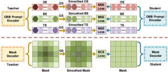
Figure 4: The process of KD for the OBB prompt encoder and mask decoder. “TE“, “BE“ and “OE“ represent encoded feature embeddings with respect to the top-left point, bottom-right point and orientation of an OBB, respectively. “GS“ stands for Gaussian smoothing.

We define a one-dimensional Gaussian kernel $\mathbf{G}^{1}_{k}(x_{i};\sigma)$ with a length of $k$, which is given as

$$\mathbf{G}^{1}_{k}(x_{i};\sigma)=\frac{1}{\mathbf{G}^{1}_{s}}e^{-[\frac{(x_{i}-x_{c})^{2}}{2\sigma^{2}}]},$$ (14)

where

$$\mathbf{G}^{1}_{s}=\sum_{i}e^{-[\frac{(x_{i}-x_{c})^{2}}{2\sigma^{2}}]},~{}~{}i\in\{0,1,\ldots,k-1\}.$$ (15)

The $x_{i}$ and $x_{c}$ represent the position of each element and the central position, respectively. $\sigma$ is the standard deviation. Given the encoded feature embeddings of the teacher model with respect to the top-left point ($\mathcal{E}^{t}(\bm{\varphi}_{1})\in\mathbb{R}^{2l}$, $l=l_{p}=l_{\theta}$), bottom-right point ($\mathcal{E}^{t}(\bm{\varphi}_{2})\in\mathbb{R}^{2l}$) and orientation ($\mathcal{E}^{t}(\bm{\theta})\in\mathbb{R}^{2l}$), we perform Gaussian smoothing by convolving the Gaussian kernel $\mathbf{G}^{1}_{k}$ with these encoded embeddings.

$$\bm{G}^{t}(\bm{\varphi}_{1}) =\mathbf{G}^{1}_{k}\circledast\mathcal{E}^{t}(\bm{\varphi}_{1}),$$ (16)

$$\bm{G}^{t}(\bm{\varphi}_{2}) =\mathbf{G}^{1}_{k}\circledast\mathcal{E}^{t}(\bm{\varphi}_{2}),$$ (17)

$$\bm{G}^{t}(\bm{\theta}) =\mathbf{G}^{1}_{k}\circledast\mathcal{E}^{t}(\bm{\theta}).$$ (18)

Then, the corresponding encoded feature embeddings ($\mathcal{E}^{s}(\bm{\varphi}_{1}),\mathcal{E}^{s}(\bm{\varphi}_{2}),\mathcal{E}^{s}(\bm{\theta})$) of the student model mimic the smoothed feature embeddings ($\bm{G}^{t}(\bm{\varphi}_{1}),\bm{G}^{t}(\bm{\varphi}_{2}),\bm{G}^{t}(\bm{\theta})$) of the teacher model. The mean squared error (MSE) loss ($\mathcal{L}_{\mathrm{prompt}}$) is used as the loss function.

$$\mathcal{L}_{\mathrm{prompt}} =\frac{1}{2l}{||\bm{G}^{t}(\bm{\varphi}_{1})-\mathcal{E}^{s}(\bm{\varphi}_{1})||}^{2}_{2}$$

$$+\frac{1}{2l}{||\bm{G}^{t}(\bm{\varphi}_{2})-\mathcal{E}^{s}(\bm{\varphi}_{2})||}^{2}_{2}$$

$$+\frac{1}{2l}{||\bm{G}^{t}(\bm{\theta})-\mathcal{E}^{s}(\bm{\theta})||}^{2}_{2}.$$ (19)

For KD on the mask decoder of a BSM, Gaussian smoothing makes the transition between boundary regions of different classes smoother and improves generalization capability. As the mask is two-dimensional, a two-dimensional Gaussian kernel $\mathbf{G}^{2}_{k\times k}(u_{i},v_{j};\delta)$ with a size of $k\times k$ is given as

$$\mathbf{G}^{2}_{k\times k}(u_{i},v_{j};\delta)=\frac{1}{\mathbf{G}^{2}_{s}}e^{-[\frac{(u_{i}-u_{c})^{2}+(v_{j}-v_{c})^{2}}{2\delta^{2}}]},$$ (20)

where

$$\mathbf{G}^{2}_{s}=\sum_{i}\sum_{j}e^{-[\frac{(u_{i}-u_{c})^{2}+(v_{j}-v_{c})^{2}}{2\delta^{2}}]},~{}~{}i,j\in\{0,1,\ldots,k-1\}.$$ (21)

The ($u_{i},v_{j}$) and ($u_{c},v_{c}$) represent the position of each element and the central position, respectively. $\delta$ is the standard deviation. In KD for segmentation tasks, unlike current methods [23, 25] that apply Gaussian smoothing to GT labels, we apply it to masks generated by the teacher model.

Since the detected OBBs distinguish instances and identify classes, the output mask is only responsible for distinguishing between foreground and background and has a shape of ($H,W$), where $H$ and $W$ represent the height and width of the input image, respectively. Given the output $\bm{M}^{t}$ of the mask decoder of the teacher model, we first use the sigmoid function $\sigma(\cdot)$ to generate a foreground probability map, and then convolve it with the Gaussian kernel $\mathbf{G}^{2}_{k\times k}$.

$$\bm{G}(\bm{M}^{t})=\sigma(\bm{M}^{t})\circledast\mathbf{G}^{2}_{k\times k},$$ (22)

Subsequently, the generated smoothed target $\bm{G}(\bm{M}^{t})$ serves as the supervision target for the corresponding probability map ($\sigma(\bm{M}^{s})$) of the mask decoder of the student model. We use the binary cross entropy (BCE) loss ($\mathcal{L}_{\mathrm{mask}}$) as the loss function, which is described as

$$\mathcal{L}_{\mathrm{mask}}=-\frac{1}{HW}\sum_{m^{t},m^{s}}[m^{t}\log m^{s}+(1-m^{t})\log(1-m^{s})],$$

$$m^{t}\in\bm{G}(\bm{M}^{t}),m^{s}\in\sigma(\bm{M}^{s}).$$ (23)

Hence, the final distillation loss ($\mathcal{L}_{\mathrm{total}}$) is

$$\mathcal{L}_{\mathrm{total}}=\lambda\cdot\mathcal{L}_{\mathrm{prompt}}+(1-\lambda)\cdot\mathcal{L}_{\mathrm{mask}},$$ (24)

where $\lambda$ is the trade-off factor between the distillation loss of the OBB prompt encoder and that of the mask decoder.

IV Experiments

IV-A Dataset

To verify the effectiveness of the proposed methods, we conduct completely occluded object IS and dense object IS experiments on self-collected industrial and publicly available datasets, respectively.

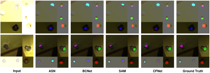
Figure 5: Some visualization results on the completely occluded object IS dataset. Bounding boxes of different colors and segmentation masks of different colors represent different object classes and different instances, respectively.

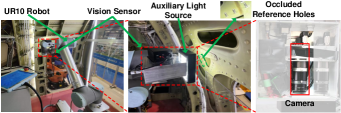
Figure 6: Self-designed robotic vision system for completely occluded object IS in the industrial environment of the large commercial aircraft C919.

IV-A1 Industrial Dataset for Completely Occluded Objects

The self-designed industrial robotic vision system for large commercial aircraft assembly is shown in Fig. 6. It mainly consists of a UR10 robot, a vision sensor and a computer (not depicted in Fig. 6). Specifically, the UR10 robot is used to carry the vision sensor for operations. The computer is responsible for receiving and processing the image data collected by the vision sensor, and it runs the algorithm for completely occluded object IS. Due to the limited working space, reference holes are usually observed from the side.

All the images in the dataset are collected by this system, including three types of completely occluded reference holes, i.e., reference holes with bolts, nuts and untreated bolts (see the top images of Fig. 1). To reflect complex and changeable environments in the assembly process, each type of reference hole is photographed with the camera at various perspectives, distances and lighting conditions. We obtain a total of 800 images, with approximately the same number of each type. These images are divided into a training set, a validation set, and a testing set in a ratio of $7\colon 1\colon 2$ in a uniform sampling manner. All images are cropped to $1024\times 1024$. For data augmentation, all images are first flipped horizontally and vertically. Therefore, there are 2240 images in the training set, 320 images in the validation set, and 640 images in the testing set. Furthermore, the Mosaic method that randomly mixes four images is used for data augmentation.

IV-A2 Publicly Available Dataset for Dense Objects

iSAID [5] is a large-scale and densely annotated IS dataset in aerial images. It has 655,451 object instances across 15 categories. The training set, validation set and testing set contain 1411, 458 and 937 images, respectively. All images are cropped into $1024\times 1024$ patches with a stride of 500. Since iSAID dataset does not provide the GT parameters of OBBs, the smallest OBBs of instance masks are used as regression targets. We only choose densely distributed large vehicles, small vehicles and ships as targets for dense object IS.

IV-B Implementation Details

The training settings for Oriented R-CNN [15] are the same as the original method. In the OBB prompt encoder, the length of the sampled Fourier basis frequencies is 128. For KD, the teacher model (called CFNet*) is based on SAM with the powerful ViT-H image encoder and the proposed OBB prompt encoder. The student model (i.e., CFNet) uses a lightweight pretrained ViT-Tiny image encoder and OBB prompt encoder. Their mask decoders and OBB detection modules are the same. During training, the weights of their image encoders are frozen, and the other parts are fine-tuned. The teacher model has the same training loss as SAM and has been trained before distillation. The trade-off factor $\lambda$ for the distillation loss is 0.2. More implementation details can be found in our open-source code at https://github.com/zhen6618/OBBInstanceSegmentation. All experiments are conducted on an RTX 3080Ti GPU. For evaluation, we use the standard COCO metrics: AP (i.e., AP_50-95, averaged over IoU threshold), AP₅₀ and AP₇₅.

IV-C Completely Occluded Object Instance Segmentation

In completely occluded object IS experiments, we compare CFNet, SAM, and amodal methods. SAM uses the ViT-H to encode images and the HBB detection branch of Mask R-CNN to generate HBB prompts (the same below). Amodal methods directly predict the unoccluded and occluded parts of the occludee instances. CFNet and SAM perform ISPBB on occluders to obtain occludee instances. We also include SAM after fine-tuning on this dataset and the teacher model (CFNet*) used for distillation in the comparison. For fair comparison, we replace the backbones of current amodal IS methods with the ViT-H image encoder used in BSMs.

TABLE I: Comparison results on the completely occluded object IS dataset. $\dagger$ represents using ViT-H as the backbone.

Method	AP	AP50	AP75	FPS
AmodalMask [17]	19.49	35.18	24.36	16.1
ASN [7]	40.88	61.24	45.93	18.6
ORCNN [8]	37.60	57.78	40.16	22.2
BCNet [6]	45.30	65.13	51.79	7.4
BCNet$\dagger$	50.09	69.30	56.42	2.7
SAM [14]	26.15	42.74	30.28	2.8
Fine-tuned SAM	68.66	82.23	71.38	2.8
CFNet*	75.13	89.21	77.98	2.7
CFNet	73.46	86.48	76.20	20.4

As shown in Table I, the IS accuracy of CFNet and CFNet* is superior to other methods, especially for high-precision metrics. CFNet exhibits competitive inference speed. Some visualization results are presented in Fig. 5. Compared with amodal IS methods, CFNet provides an effective solution for completely occluded IS by performing ISPBB on occluders. In addition, compared with fine-tuned SAM using HBBs, the IS accuracy of CFNet and CFNet* using OBBs is significantly improved, which indicates the necessity of using OBBs. Moreover, our proposed KD method significantly improves the inference speed with a minor loss in accuracy.

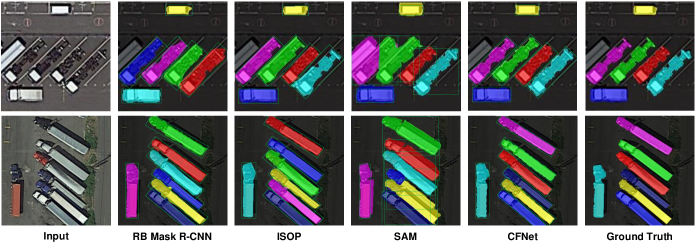
Figure 7: Some visualization results on the dense object IS dataset iSAID. Bounding boxes of different colors and segmentation masks of different colors represent different object classes and different instances, respectively.

IV-D Dense Object Instance Segmentation

For dense object IS, we compare CFNet, SAM, and current IS methods using OBBs. Additionally, Mask R-CNN using HBBs is added for comparison. We also include fine-tuned SAM and the teacher model used for distillation in the comparison, and replace the backbones of current IS methods using OBBs with the ViT-H image encoder used in BSMs.

TABLE II: Comparison results on the Dense object IS dataset. “RB Mask R-CNN“ represents Rotated Blend Mask R-CNN [10].

Method	AP	AP50	AP75	FPS
Mask R-CNN [3]	13.65	37.23	18.15	25.0
OIS [11]	27.41	47.85	30.71	18.4
RB Mask R-CNN [10]	29.07	50.96	32.64	16.3
ISOP [19]	34.73	59.16	36.84	19.6
ISOP$\dagger$	37.81	61.95	39.45	2.7
SAM [14]	14.37	41.88	18.52	2.8
Fine-tuned SAM	20.26	45.30	24.59	2.8
CFNet*	45.10	66.45	47.92	2.7
CFNet	43.76	64.29	46.13	20.4

As presented in Table II, CFNet and CFNet* outperform other methods, and CFNet achieves a competitive inference speed of 20.4 FPS. In addition, CFNet achieves a remarkable dense object IS accuracy of 43.76% AP, 64.29% AP₅₀, and 46.13% AP₇₅. Fig. 7 shows some dense object IS results.

Compared with existing IS methods using OBBs, CFNet achieves higher accuracy since it reduces the dependence on OBBs and is based on BSMs. Significant accuracy improvements over fine-tuned SAM also indicate the benefit of using OBBs. Moreover, compared with CFNet*, the notable speed improvement and minor accuracy loss of CFNet also demonstrate the effectiveness of the proposed KD method.

IV-E Ablation Studies

To evaluate the effectiveness of the components of CFNet, a series of ablation experiments are conducted on the iSAID dataset. We use the most commonly used AP₅₀ as the metric.

IV-E1 Oriented Bounding Box Prompt Encoder

The OBB prompt encoder introduces positional encoding and specific embeddings to encode OBBs. We analyze them in Table III. “OCE“, “TCE“ and “BCE“ represent the specific orientation correction embeddings, top-left corner embeddings and bottom-right corner embeddings, respectively. Compared with GPE, AGPE encodes location information better by adaptively learning parameters of Gaussian distributions. Specific embeddings further improve IS performance.

TABLE III: Performance of each component of the OBB prompt encoder.

GPE	AGPE	TCE+BCE	OCE	AP50
✓				61.40
	✓			62.27
	✓	✓		63.56
	✓	✓	✓	64.29

TABLE IV: Comparison of different learning targets and label smoothing methods in KD.

	GT+ULS	GT+GS	T+GT	T	T+ULS	T+GS
AP50	63.51	63.72	64.01	64.07	64.15	64.24

IV-E2 Knowledge Distillation

We first compare the performance of CFNet learning from the teacher model and GT labels, and test the impact of different label smoothing methods. “T“ represents learning from the teacher model. The smoothing factor in ULS is 0.1. Gaussian smoothing (GS) has the same settings as SVLS, with a Gaussian kernel size of $3\times 3$ and a standard deviation of 1.0. The weight factor of the teacher model and GT labels is 0.1.

The experimental results in Table IV demonstrate that learning from the teacher model has higher performance than learning from GT labels (learning only from GT labels means no KD is performed), which is mainly due to the powerful data-fitting capabilities of BSMs. Moreover, Gaussian smoothing further improves IS performance and is superior to ULS. In addition, we compare the impact of different parameter settings in Gaussian smoothing on IS performance in Table V. When $k=5$, $\sigma=0.3$, and $\delta=1.0$, the highest IS accuracy of 64.29% AP₅₀ is achieved.

TABLE V: Impact of different parameter settings in Gaussian smoothing on IS performance.

	$\sigma=0.3$		$\sigma=0.5$
	$\delta=0.5$	$\delta=1.0$	$\delta=0.5$	$\delta=1.0$
$k=3$	64.24	64.24	64.20	64.17
$k=5$	64.22	64.29	64.18	64.21
$k=7$	64.19	64.25	64.15	64.14

IV-E3 Oriented Bounding Box Detection

To explore the impact of the OBB detection module on the IS performance, we compare Oriented R-CNN used in CFNet with some other OBB detection methods [27, 28]. Additionally, a HBB detection method (HBB detection branch of Mask R-CNN) is also added for comparison. As shown in Table VI, the effective use of OBBs significantly improves IS accuracy, and CFNet is not sensitive to specific OBB detection methods.

TABLE VI: Performance comparison of OBB and HBB detectors.

	Mask	Oriented	Oriented	S2ANet [28]
	R-CNN [3]	R-CNN [15]	Reppoints [27]
AP50	42.95	64.29	64.37	64.06

V Conclusions

This paper proposes CFNet, a coarse-to-fine IS framework for completely occluded and dense objects. Specifically, CFNet is based on BSMs and introduces a novel OBB prompt encoder. To make CFNet more lightweight, a KD method using Gaussian smoothing for soft teacher targets is applied to the OBB prompt encoder and mask decoder. Experimental results on both industrial and publicly available datasets demonstrate that CFNet outperforms all tested methods. One limitation of this work is that CFNet relies on prior geometric properties to achieve completely occluded object IS. We plan to utilize multiple types of prior knowledge to achieve more robust IS in more complex scenarios.

References

- [1] Y. Liu, X. Chen, and P. Abbeel, “Self-supervised instance segmentation by grasping,” in IEEE Int. Conf. Intell. Robots Syst., 2023, pp. 1162–1169.
- [2] Z. Dong, S. Liu, T. Zhou, H. Cheng, L. Zeng, X. Yu, and H. Liu, “Ppr-net:point-wise pose regression network for instance segmentation and 6d pose estimation in bin-picking scenarios,” in IEEE Int. Conf. Intell. Robots Syst., 2019, pp. 1773–1780.
- [3] K. He, G. Gkioxari, P. Dollar, and R. Girshick, “Mask r-cnn,” in IEEE Int. Conf. Comput. Vis., Oct 2017.
- [4] F. Li, H. Zhang, H. Xu, S. Liu, L. Zhang, L. M. Ni, and H.-Y. Shum, “Mask dino: Towards a unified transformer-based framework for object detection and segmentation,” in IEEE Int. Conf. Comput. Vis. Pattern Recognit., June 2023, pp. 3041–3050.
- [5] S. Waqas Zamir, A. Arora, A. Gupta, S. Khan, G. Sun, F. Shahbaz Khan, F. Zhu, L. Shao, G.-S. Xia, and X. Bai, “isaid: A large-scale dataset for instance segmentation in aerial images,” in IEEE Int. Conf. Comput. Vis. Pattern Recognit. Workshops, June 2019.
- [6] L. Ke, Y.-W. Tai, and C.-K. Tang, “Occlusion-aware instance segmentation via bilayer network architectures,” IEEE Trans. Pattern Anal. Mach. Intell., vol. 45, no. 8, pp. 10 197–10 211, 2023.
- [7] L. Qi, L. Jiang, S. Liu, X. Shen, and J. Jia, “Amodal instance segmentation with kins dataset,” in IEEE Int. Conf. Comput. Vis. Pattern Recognit., June 2019.
- [8] P. Follmann, R. König, P. Härtinger, M. Klostermann, and T. Böttger, “Learning to see the invisible: End-to-end trainable amodal instance segmentation,” in IEEE Winter Conf. Appl. Comput. Vis., 2019, pp. 1328–1336.
- [9] K. Li and J. Malik, “Amodal instance segmentation,” in Eur. Conf. Comput. Vis., 2016, pp. 677–693.
- [10] Z. Zhang and J. Du, “Accurate oriented instance segmentation in aerial images,” in Int. Conf. Image Graphics, 2021, pp. 160–170.
- [11] P. Follmann and R. König, “Oriented boxes for accurate instance segmentation,” in arXiv preprint arXiv:1911.07732, 2020.
- [12] Y. Feng, B. Yang, X. Li, C.-W. Fu, R. Cao, K. Chen, Q. Dou, M. Wei, Y.-H. Liu, and P.-A. Heng, “Towards robust part-aware instance segmentation for industrial bin picking,” in IEEE Int. Conf. Robot. Autom., 2022, pp. 405–411.
- [13] C. Zhang, D. Han, Y. Qiao, J. U. Kim, S.-H. Bae, S. Lee, and C. S. Hong, “Faster segment anything: Towards lightweight sam for mobile applications,” in arXiv preprint arXiv:2306.14289, 2023.
- [14] A. Kirillov, E. Mintun, N. Ravi, H. Mao, C. Rolland, L. Gustafson, T. Xiao, S. Whitehead, A. C. Berg, W.-Y. Lo, P. Dollar, and R. Girshick, “Segment anything,” in IEEE Int. Conf. Comput. Vis., October 2023, pp. 4015–4026.
- [15] X. Xie, G. Cheng, J. Wang, X. Yao, and J. Han, “Oriented r-cnn for object detection,” in IEEE Int. Conf. Comput. Vis., October 2021, pp. 3520–3529.
- [16] P. O. Pinheiro, T.-Y. Lin, R. Collobert, and P. Dollár, “Learning to refine object segments,” in Eur. Conf. Comput. Vis., 2016, pp. 75–91.
- [17] Y. Zhu, Y. Tian, D. Metaxas, and P. Dollar, “Semantic amodal segmentation,” in IEEE Int. Conf. Comput. Vis. Pattern Recognit., July 2017.
- [18] Y. Yan, Y. Qi, C. Xu, N. Su, and L. Yang, “Building extraction at amodal-instance- segmentation level: Datasets and framework,” IEEE Trans. Geosci. Remote Sens., vol. 62, pp. 1–18, 2024.
- [19] T. Pan, J. Ding, J. Wang, W. Yang, and G.-S. Xia, “Instance segmentation with oriented proposals for aerial images,” in IEEE Int. Geosci. Remote Sens. symp., 2020, pp. 988–991.
- [20] Y. Huang, X. Yang, L. Liu, H. Zhou, A. Chang, X. Zhou, R. Chen, J. Yu, J. Chen, C. Chen, S. Liu, H. Chi, X. Hu, K. Yue, L. Li, V. Grau, D.-P. Fan, F. Dong, and D. Ni, “Segment anything model for medical images?” Med. Image Anal., vol. 92, p. 103061, 2024.
- [21] M. Tancik, P. Srinivasan, B. Mildenhall, S. Fridovich-Keil, N. Raghavan, U. Singhal, R. Ramamoorthi, J. Barron, and R. Ng, “Fourier features let networks learn high frequency functions in low dimensional domains,” in Adv. Neural Inf. Process. Syst., vol. 33, 2020, pp. 7537–7547.
- [22] C. Szegedy, V. Vanhoucke, S. Ioffe, J. Shlens, and Z. Wojna, “Rethinking the inception architecture for computer vision,” in IEEE Int. Conf. Comput. Vis. Pattern Recognit., June 2016.
- [23] M. Islam and B. Glocker, “Spatially varying label smoothing: Capturing uncertainty from expert annotations,” in Inf. Process. Med. Imag., 2021, pp. 677–688.
- [24] S. Park, J. Kim, and Y. S. Heo, “Semantic segmentation using pixel-wise adaptive label smoothing via self-knowledge distillation for limited labeling data,” Sensors, vol. 22, no. 7, 2022.
- [25] M. Islam, L. Seenivasan, S. P. Sharan, V. K. Viekash, B. Gupta, B. Glocker, and H. Ren, “Paced-curriculum distillation with prediction and label uncertainty for image segmentation,” in Int. J. Comput. Assisted Radiology surg., vol. 18, 2023, pp. 1875–1883.
- [26] X. Yang, G. Zhang, X. Yang, Y. Zhou, W. Wang, J. Tang, T. He, and J. Yan, “Detecting rotated objects as gaussian distributions and its 3-d generalization,” IEEE Trans. Pattern Anal. Mach. Intell., vol. 45, no. 4, pp. 4335–4354, 2023.
- [27] W. Li, Y. Chen, K. Hu, and J. Zhu, “Oriented reppoints for aerial object detection,” in IEEE Int. Conf. Comput. Vis. Pattern Recognit., June 2022, pp. 1829–1838.
- [28] J. Han, J. Ding, J. Li, and G.-S. Xia, “Align deep features for oriented object detection,” IEEE Trans. Geosci. Remote Sens., vol. 60, pp. 1–11, 2022.