MaRTIn

Abstract

We present MaRTIn, an extendable all-in-one package for calculating amplitudes up to two loops in an expansion in external momenta or using the method of infrared rearrangement. Renormalizable and non-renormalizable models can be supplied by the user; an implementation of the Standard Model is included in the package. In this manual, we discuss the scope and functionality of the software, and give instructions of its use.

tableofcontents.1tableofcontents.1Table of ContentsTable of Contentstableofcontents.1

1 Overview

Perturbation theory is one of the most reliable tools to obtain quality predictions from quantum field theories. In order to further enhance the precision, higher loop orders are required, increasing the computational complexity of the calculation and with it the need for more sophisticated software pipelines to automatise them. Traditionally, these tool chains follow a modular structure, though not all pieces or build scripts are public. For instance, generic Feynman diagrams can be generated via QGRAF [1], Feynarts [2, 3] or future versions of FORM [4, 5]. These expressions require further manipulation such as inserting Feynman rules, problem-specific diagram filtering and expansions, partial fractioning, tensor reduction and topology identification. Subsets of these tasks can be delegated to tools like DIANA [6], q2e and exp [7, 8], LIMIT [9], tapir [10], TopoID [11], Alibrary [12] and Feynson [13]. Moreover, the algebra of spinor contractions and symmetry groups has to be simplified. Note that there is a plethora of software packages automatising computations at tree-level and one-loop order, employing a Passarino–Veltman decomposition of integrals [14]. However, already at two loops a more sophisticated methodology is required. Integration-by-parts (IBP) relations are recursively applied to loop integrals until they have reduced to master integrals. This step may be performed by LiteRed [15, 16], FIRE [17, 18, 19, 20], Reduze [21, 22] or Kira [23, 24]. Examples of packages combining the IBP reductions and insertion of master integrals for specific families of problems are MINCER [25], MATAD [26], FORCER [27] and FMFT [28].

MaRTIn (Massive Recursive Tensor Integration) aims to be an all-in-one tool for the computation of multi-leg amplitudes in an expansion of small external momenta at tree and loop level in arbitrary quantum field theories. A typical computation starts from Feynman rules specified by the user, which may comprise both renormalisable and non-renormalisable operators. MaRTIn leverages QGRAF [1] to generate Feynman diagrams automatically, and proceeds with the main computation using routines implemented in FORM [4, 5]. This includes the resolution of spinor, gauge, and global symmetry index contractions, as well as the tensor and IBP reduction and, eventually, scalar loop integration. Several schemes for the treatment $\gamma_{5}$ are available.

The major mode of operation employs either an expansion in all external momenta, or the infrared rearrangement outlined in Refs. [29, 30]. In either case, integrals are reduced to vacuum topologies with arbitrary, possibly vanishing mass arguments. The integration is then performed symbolically up to two-loop order in $4-2\varepsilon$ space-time dimensions [31, 32], to a user-specified order in powers of $\varepsilon$ and external momenta. The functionality to perform calculations in $3-2\varepsilon$ space-time dimensions is contained in the package, but is not as well-tested.

Another mode of operation retains the full momentum dependence but does not perform any integration. This is implemented up to one-loop order. The functionality of MaRTIn may be extended in future releases.

MaRTIn produces outputs in both FORM and Mathematica [33] compatible formats, and optionally a graphical representation of all involved Feynman diagrams.

In the following sections, we specify in detail how MaRTIn is obtained, installed, operated, and extended.

2 Setup

MaRTIn is distributed under the GNU Public License, Version 3 [34] and available to download at https://gitlab.com/manstam/martin. The code itself is mostly written in and tested against FORM 4 [5], which has to be installed separately. Similarly, MaRTIn requires QGRAF [1] to generate diagrams. Note that both packages have several subdependencies and need to be compiled from their source codes. Thus, a POSIX compatible system with a working GNU toolchain is required. MaRTIn is operated using GNU make as well as a python3 script, which in turn requires the common modules os, sys, shutil, re, argparse, subprocess and configparser. The underlying Makefile also utilises bash, (GNU) awk and several other standard shell programs. In order to output Feynman diagrams in PDF format, graphviz with the neato engine are required. Optionally, the package richard_draw may be utilised, which produces higher-quality output using lualatex. It can be downloaded at https://gitlab.com/manstam/richard_draw.

Once all prerequisites are met, MaRTIn needs to be set up in three places:

• The source code directory martin. It requires no further installation, but a system soft link to the main executable martin/martin.py is recommended. The source directory includes the subdirectories code with the source codes, user_template with some prototypes of the files, and further directories mentioned below, as well as this manual.

• A config file .martin.conf, which should be manually placed in the user’s home directory. A template version of the file is contained in
  martin/user_template/template_martin.conf. This file specifies the locations to the FORM and QGRAF executables, the number of default parallel processes, FORM options and default paths. The options are detailed in the template file itself.

• The user’s working directory, e.g., named martin_user, which should be created by the user and populated with the following subdirectories
  (examples are found in martin/user_template):

  • models: This directory contains all user-defined model files. Further details are deferred to Sec. 4.

  • problems: contains (possibly nested) subdirectories, which can have arbitrary names. Each of these subdirectories may contain several loop.*.dat files. Every such file specifies all options required for a single run of MaRTIn. The contents of these files will be explained in Sec. 3.

  • prc: is the canonical location for user-defined FORM routines that will be automatically detected by MaRTIn. The routines can then be included in the FORM folds of the model or loop.*.dat files (see Sec. 3.1).

  • results: This is the location were MaRTIn automatically writes intermediate and final output, creating the same folder structure as in the user-defined problems directory. The user should not manually modify or add to the contents of this directory since MaRTIn’s functionality can overwrite and delete these directories.

In order to test whether the MaRTIn installation is complete, users can calculate the example described in greater detail in Sec. 5. All files necessary for this run are contained in MaRTIn. Assuming that FORM, QGRAF, and MaRTIn are properly set up, the command

⬇

martin ./user_template/problems/SM/loop.1_uu.dat

invoked from the main MaRTIn directory should generate and compute the diagram in Fig. 1. The command

⬇

martin ./user_template/problems/SM/loop.1_uu.dat pdf

should generate a pdf file of the corresponding diagrams. Using rpdf instead of the target pdf would instead use richard_draw to create a pdf file for the diagrams. A successful run will provide the screen printout discussed in Sec. 5, and save all results in the directory ./user_template/results/SM/.

In the next section, we describe the concrete workflow of MaRTIn in detail.

3 Workflow

Input files	Output files
QGRAF files (diagrams)    models/qgraf/model.prop.lag    models/qgraf/model.vrtx.lag FORM model file (Feynman rules)    models/form/model_MODEL Problem file (process and options)    problems/process/loop.problem.dat Optional: richard_draw file (drawing)    models/rdraw/model.json	FORM output    results/process/form.problem/dia*.sav Mathematica output    results/process/math.problem/dia*.m Feynman graphs    results/process/graphs.problem.pdf richard_draw Feynman graphs    results/process/rgraphs.problem.pdf

Table 1: Overview of MaRTIn input and output files. See text for details.

In this section we describe how MaRTIn is used. A list of the required input files, as well as the output files, is contained in Tab. 1. The two key elements for the operation of MaRTIn are the loop.problem.dat, which contains all information about the calculation at hand, as well as the main executable martin.py, which serves as a convenience wrapper around the Makefile. Note that problem here represents a placeholder for a user-defined identifier. Different steps of the computation are triggered by targets arguments passed to the executable. Assuming that the full path to martin.py has been aliased as the command martin, a typical MaRTIn call has the following shape:

⬇

martin problems/process/loop.problem.dat targets

The command

⬇

martin -h

lists and explains all target options. There are many targets that are only important for the inner workings of MaRTIn and are evaluated successively. By default, output of all targets (including intermediate ones) are written to the directory results/process/. For the user, the most relevant targets are the following:

• all is the default target of martin.py and will be called if no target argument is specified. It computes all diagrams and saves the results in the results folder, as discussed above. For every diagram that has not been computed already, MaRTIn will spawn a separate process to do so. The maximal number of parallel processes can be configured in .martin.config.

• diaNUM computes the single diagram with number NUM. The result is written to results/process/form.problem/diaNUM.sav using FORMs binary format, as well as results/process/math.problem/diaNUM.m in Wolfram Language.

• sum computes the sum of all Feynman diagrams. The results are stored as results/process/form.problem/diasum.sav in FORM as well as
  results/process/math.problem/diasum.m in Mathematica compatible format. If any individual diaNUM.sav files are missing, they will be computed with the all target.

• pdf will generate a PDF file containing the graphical representation of each Feynman diagram. This is stored in results/process/graphs.problem.pdf.

• rpdf utilises richard_draw to generate a higher-quality pdf file containing all Feynman graphs. This is stored under results/process/rgraphs.problem.pdf.

• clean removes all final and intermediate results of the selected problem.

The executable martin.py also takes arguments that can be used to override options in the config file .martin.conf, call martin -h for further details. In the remainder of this section, we specify the content and structure of a valid loop.problem.dat file, before giving an overview of MaRTIn’s algorithm.

3.1 Problem file

The file problems/process/loop.problem.dat contains all necessary information for a single run of MaRTIn. It specifies how the model is assembled from the modular pieces that will be introduced in Sec. 4, defines in detail which Feynman diagrams are to be calculated, configures various aspects of the computation itself, and specifies if and how user-defined code is injected. Example files can be found in the MaRTIn source directory at user_template/problems/SM/.

The file itself consists of FORM folds, i.e. named objects of the syntax

⬇

*--#[ FOLDNAME :

some code here

*--#] FOLDNAME :

which are being inserted at the right place by FORM’s preprocessor. These objects must never be deleted from the file, even if they are empty. The content of each fold is FORM code. The only exception is the very first fold we encounter, which actually contains QGRAF’s own scripting language. In fact, this fold contains the contents of the QGRAF input file:

⬇

*--#[ QGRAF :

*   This is a comment.

*   Do not remove or reorder statements below.

*   Define which QGRAF model files to use.

*   We typically split them into propagators and vertices, but that is not required.

*   Both are should be valid files located in models/qgraf/

*   The functionality of including multiple models in this

*   way is a MaRTIn feature; it is not possible in solo QGRAF runs

model = "qmodel.prop.lag";

model = "qmodel.vrtx.lag";

*   Define external legs using field names.

*   Use q’s for external momenta (note that martin substitutes q0 = 0.

in = field1[q1], field2[q2];

out = field3[q3], field4[q4];

*   Loop order, e.g. 2. Loop momenta have to be p1, p2.

loops = 2;

loop_momentum = p;

*   Some options to select topologies, e.g.:

options = onepi;

*   More selectors like vsums and psums here

*--#] QGRAF :

Note that MaRTIn allows for the presence of several separate QGRAF model files; they are combined automatically before being passed to QGRAF by concatenating (cat) them in the order they appear in the fold. It is the user’s responsibility to ensure that the model files are consistent with each other. We refer to the QGRAF manual for a more detailed description of the valid syntax.

The next fold sets up important options for the FORM part of MaRTIn. These are saved as preprocessor variables, which are collected and described in Tab. 2. An example and more explanations are given below.

Option	Description
NM	Represents the number of FORM model files that are
	being combined for the current problem.
MODELi	Series of variables with integer i going from 1 to NM.
	Each refers to a filename model_MODELx of a
	FORM model file found in models/form/.
EXPDENO	Before integration, expand in external momenta to a
	power given by this variable. This option is
	exclusive with IRA and GENERICLOOPFUNCTIONS.
IRA	Perform infrared rearrangement before integration.
	Expand external momenta up to a power specified by
	this variable. Exclusive option with EXPDENO and
	GENERICLOOPFUNCTIONS.
GENERICLOOPFUNCTIONS	Skip integration, collect integrand in generic function.
	Exclusive option with EXPDENO and IRA.
FINALEPLIM	Power in $\varepsilon$ up to which the final result is expanded.
DSCHEME	Scheme for handling $\gamma_{5}$. Options are "NDR" (default),
	"sNDR", "HV" and "LARIN". See main text for details.
CLLABEL	If defined, mark each closed fermion loop with a function
	cl tracking the fields in the loop.
PRINT	If defined, intermediate steps in the computation of
	each diagram are printed to the terminal.
FINALPRINT	If defined, the final result of each diagram is printed
	to the terminal.

Table 2: Overview of preprocessor options to configure MaRTIn. These are found in the fold MAIN located in each problem file.

⬇

*--#[ MAIN :

*   This is a FORM comment.

*   Each model may consist of several form model files found in models/form/

*   The total number of model files must be given as NM.

*   For instance, for two model files with names ‘‘model_fmodelA’’ and ‘‘model_fmodelB’’:

#define NM "2"

#define MODEL1 "fmodelA"

#define MODEL2 "fmodelB"

*** Modes of operation. Only one of these three should be defined.

*   Expand in external momenta to this power

#define EXPDENO "2"

*   Define if infrared rearrangement should be used.

#define IRA "1"

*   No integration, keep a generic expression of unsolved integrals

#define GENERICLOOPFUNCTIONS

Defining EXPDENO "$n$" will perform a Taylor expansion of all propagators $\frac{1}{(p+q)^{2}-m^{2}}$ up to powers $n$ in all external momenta $q$. Alternatively, setting the option IRA ‘‘$n$’’ the code performs an infrared rearrangement [29, 30], i.e., it introduces the regularising mass parameter $m_{\text{IRA}}$ via the repeated application of the identity

$$\frac{1}{(p+q)^{2}-M^{2}}=\frac{1}{p^{2}-m_{\text{IRA}}^{2}}+\frac{M^{2}-m_{\text{IRA}}^{2}-2\,p\!\cdot\!q-q^{2}}{p^{2}-m_{\text{IRA}}^{2}}\frac{1}{(p+q)^{2}-M^{2}}\,.$$ (1)

External momenta are kept up to power $n$. In practice, this identity is applied recursively to every term until its degree of divergence is negative; these terms are then dropped. Note that the $m_{\text{IRA}}^{2}$ in the numerator of the second term on the right side of the equation is dropped; accordingly, additional local counterterms must be introduced (see Ref. [30] for details).

⬇

*   Order in $\varepsilon$ to which final result is expanded

*   This is not relevant for the GENERICLOOPFUNCTIONS option

#define FINALEPLIM "-1"

*** Scheme how gamma5 should be treated. The options are:

*   NDR -- naive dimensional regularisation, abort on gamma5 encounter inside traces

*   sNDR -- semi-naive dimensional regularisation, use naive relations

*   sNDR -- in $(4-2\varepsilon)$ dimensions, but set flagsNDR

*   HV -- Breitenlohner - Maison - ’t Hooft - Veltman treatment

*   LARIN -- Larin’s scheme: replace gamma5 by Levi-Civita contraction

#define DSCHEME "NDR"

A few comments about the implemented $\gamma_{5}$ schemes are in order. The issues with $\gamma_{5}$ arise due to the choice of dimensional regularisation [35]. The $\gamma_{5}$ matrix is defined as

$$\gamma_{5}=\frac{i}{4!}\epsilon_{\mu\nu\rho\sigma}\,\gamma^{\mu}\gamma^{\nu}\gamma^{\rho}\gamma^{\sigma}\,,$$ (2)

where $\epsilon_{\mu\nu\rho\sigma}$ denotes the completely antisymmetric Levi-Civita tensor in four space-time dimensions, with the convention $\epsilon_{0123}=1$.

It is well known that the anticommutation relation

$$\{\gamma_{5},\gamma^{\mu}\}=0$$ (3)

is algebraically inconsistent with the trace operation in $d\neq 4$ space-time dimensions [36]. In order enable consistent treatments of $\gamma_{5}$, MaRTIn internally can keep track of whether fermion lines are open or closed, how many $\gamma_{5}$ appear, and whether Lorentz indices are $(4-2\varepsilon)$-, $4$- or $(-2\varepsilon)$-dimensional. The following options to handle $\gamma_{5}$ are currently implemented:

• #define DSCHEME "NDR" : “Naive dimensional regularisation”
  This is the default choice of the algorithm. If $\gamma_{5}$ is encountered inside a trace, MaRTIn exits with an error since NDR can give algebraically inconsistent results in traces. In open fermion lines, $\gamma_{5}$ matrices are moved to the right, assuming anticommutation $\{\gamma_{5},\gamma^{\mu}\}=0$.

• #define DSCHEME "sNDR" : “Semi-Naive dimensional regularisation” [37, 38]
  This algorithm always uses the anticommutation relation in Eq. (3). Inside traces, $\gamma_{5}$ is replaced via the relation in Eq. (2), and the Levi-Civita tensors and their contractions are formally treated as $(4-2\epsilon)$-dimensional. The implication of this simplifying assumption is that only $(4-2\epsilon)$-dimensional metric tensors and $\gamma$-matrices will appear in the final result. Of course, the relation in Eq. (2) is then actually inconsistent unless additional terms $\propto\varepsilon$ are introduced, which this scheme neglects. Instead, whenever this insertion is made the term is marked by the variable flagsNDR. Thus, starting from a certain order of $\varepsilon$, the sNDR algorithm does not yield a consistent result. The highest consistent order is the first one at which flagsNDR appears. Tracking the flagsNDR dependence is the responsibility of the user.

• #define DSCHEME "HV" : “’t Hooft–Veltman scheme” [39, 40, 41, 42]
  The $\gamma_{5}$ matrix is assumed to anticommute with $\gamma^{\mu}$ if $\mu=0,1,2,3$, and to commute with $\gamma^{\mu}$, otherwise; i.e. $\left\{\gamma_{5},\,\tilde{\gamma}^{\mu}\right\}=0$ and $\left[\gamma_{5},\,\hat{\gamma}^{\mu}\right]=0$, where $\tilde{\gamma}^{\mu}$ and $\hat{\gamma}^{\mu}$ are the projections onto the $4$- and $d-4$-dimensional subspaces, respectively. Internally, projected Lorentz indices are contracted via the projected metric tensors dd, ddtilde and ddhat in $(4-2\varepsilon)$, $4$ and $(-2\varepsilon)$ dimensions, respectively. Levi-Civita tensors are treated in four integer dimensions.

• #define DSCHEME "LARIN" : “Larin scheme” [43]
  In this scheme, any instance of $\gamma_{5}$ on both open and closed fermion lines is replaced via the relation in Eq. (2) before traces are evaluated. The Levi-Civita tensor is treated in four integer dimensions.

⬇

*   Define to introduce a label for each closed fermion line.

*   Syntax: cl(line_id, field_1 , ..., field_n )

#define CLLABEL

*   Define to print the final result to the screen.

#define FINALPRINT

*   Define to get more information about intermediate steps of the calculation.

#define PRINT

*--#] MAIN :

Finally, there are several folds to inject user-defined FORM code, see also Sec. 3.2.

⬇

*--#[ USERDEF :

*   Fill with your own FORM declarations.

*--#] USERDEF :

*--#[ TEST :

*   Code injection after model definitions, but before diagrams are generated.

*--#] TEST :

*--#[ FOLD1 :

*   Code injection right after expressions for each diagram are generated.

*--#] FOLD1 :

*--#[ FOLD2 :

*   Code injection before Dirac algebra treatment.

*--#] FOLD2 :

*--#[ FOLD3 :

*   Code injection before integration.

*--#] FOLD3 :

*--#[ FOLD4 :

*   Code injection after integration.

*--#] FOLD4 :

*--#[ FOLD5 :

*   Code injection after $\varepsilon$ expansion and coupling insertion.

*   Recommendation: replace function internally used for $(\mu/M)^{2\varepsilon}$.

id eM(M?) = 1

- 2*ep*Log(M)

+ 2*ep*Log(mu)

+ 2*ep^2*Log(M)^2

+ 2*ep^2*Log(mu)^2

- 4*ep^2*Log(mu)*Log(M);

*--#] FOLD5 :

In the next section, we detail the working algorithm of MaRTIn and also show where each fold is included.

3.2 Algorithm

Simplified overview of MaRTIn’s computational pipeline. Red rounded squares represent input data, blue squares parts of the computation, and yellow ellipses indicate output files.

4 Model Definition

In the previous section, we saw that each model is defined by a set of related QGRAF and FORM model files. In this section, we will give some details on the vital components of these files, which should enable users to implement their own models.

MaRTIn uses the QGRAF and FORM model files to assemble a symbolic representation of the amplitude from the implemented Feynman rules. To achieve this, it uses the leg numbers generated by QGRAF to (i) bring spinorial terms into the correct order, (ii) generate all necessary (gauge and Lorentz) indices, and (iii) substitute all Feynman rules.

4.1 QGRAF files

The QGRAF-model files are located in the working directory at models/qgraf/. They are simply QGRAF model files, the syntax may include any elements valid for the locally installed QGRAF version. It is recommended to provide two separate files, one for all propagators and one for all vertices, named model.prop.lag and model.vrtx.lag, respectively. The reason for this is that propagators must be defined before vertices in QGRAF. Splitting each model in a propagator and a vertex part makes it possible to include multiple models. MaRTIn will then automatically combine all QGRAF model files into a single file in the correct order and pass it to QGRAF. The propagator file essentially contains several statements of the type

⬇

[Boson, BosonBar, +; pfunct=’function’, m=’mass’]

[Fermion, FermionBar, -; pfunct=’function’, m=’mass’]

where cursive words are placeholders for identifiers to be defined by the user. To be precise, the first two argument define the names of the fields and their adjoints. For real fields, both are the same. The names must be declared symbols in the FORM model file. The third argument determines if the field is fermionic or bosonic. The keyword pfunct after the semicolon is required. Its argument has to be declared as a commuting FORM function in the FORM model file and represents the propagator function. MaRTIn automatically populates its arguments with information about the propagator and its fields. Similarly, the keyword m is mandatory and represents the mass of the propagating field. It has to be a valid FORM symbol, to be declared in the FORM model file. Note that M0 is implicitly assumed to be a vanishing mass. All additional keywords, including external, are admissible. In the same manner, vertex file contains several statements of the form

⬇

[Field1, Field2, Field3, ...; vfunct=’function’]

where additional keywords are allowed. vfunct is required by MaRTIn and represents the vertex function. It has to be declared in the FORM model file as a commuting function. Note that MaRTIn provides its own QGRAF style file. The output of QGRAF is distributed into one .dot file per diagram, which are read by the FORM routine and handled in a parallelised fashion.

4.2 FORM files

The FORM model files contain the main information about the QFT at hand. While the QGRAF files define fields and specify vertices by their legs, the actual Feynman rules are implemented in the FORM model files, which MaRTIn’s gengraph routine uses to generate the amplitude. The FORM model files are located in models/form/ in the user’s working directory, and consist entirely of FORM folds. None of these folds may be omitted from the file. We recommend using an existing model file as a template for creating a new one. An empty template is provided in the MaRTIn source directory at user_template/models/form/model_MODEL. A full working example, model_SM, can be found in the same folder.

4.2.1 Internal representation of propagators and vertices

The gengraph routine uses the raw QGRAF output to generate a symbolic amplitude according to the Feynman rules implemented in the FORM model file. The essential steps comprise the generation of all group indices, insertion of the Feynman rules, and ordering of the fermion lines. In this section, we briefly describe how propagators and vertices are represented internally, and introduce MaRTIn’s fermionline objects.

All propagators and vertices are initially (i.e. before the substitution of the Feynman rules) represented by commuting functions. Their names are assigned by the pfunct and vfunct statements in the QGRAF model files. These commuting functions must be declared in the DEF fold of the FORM model file (see Sec. 4.2.8). In addition, commuting functions representing external leg factors are automatically generated. Therefore, all field (and anti-field) variables used in the QGRAF model files must also be declared as symbols in the DEF fold.

Using MaRTIn’s style file, QGRAF provides a unique description of the topology of any given Feynman diagram by providing either unique pairs of positive numbers, with one number being associated with one end of a propagator and the same number being associated with the corresponding (internal) leg of a vertex; or by providing a unique pair of negative numbers, with one number being associated with an external leg of a vertex, and the same number labeling a corresponding “polarization function”. The initial symbolic representation of any propagator function PROP is, thus, of the form

⬇

PROP($i_{1}$,$i_{2}$,mom,$p$,mass,$m$,field,$f$)

Here, $i_{1}$ and $i_{2}$ are two unique positive integers provided by QGRAF. They are followed by the momentum $p$ of the propagator, the mass $m$ of the propagator, and a symbol $f$ denoting the name of the field to which the propagator belongs. These variables are indicated by the “separator” variables mom, mass, and field, respectively. These arguments help the user identifying each propagator and inserting the correct Feynman rule.

The situation is similar for all $N$-leg vertices. Here the order of fields is the same as defined in the QGRAF model file. Any vertex function VERTEX is of the form

⬇

VERTEX($i_{1},\ldots,i_{N}$,mom,$p_{1},\ldots,p_{N}$)

where $i_{1},\ldots,i_{N}$ are unique integers provided by QGRAF, positive of negative depending on whether the corresponding leg is internal or external. mom is a separator, followed by the incoming momenta for each leg.

Finally, each external leg receives a polarization function POL of the form

⬇

POL($f$,$i$,$p$)

with $f$ again the symbol denoting the name of the corresponding field, $i$ a unique negative integer provided by QGRAF, and $p$ the momentum of the external line. Whether the momentum is incoming or outgoing depends on whether the corresponding leg/state has been chosen as incoming or outgoing in the QGRAF fold.

These representations are the starting point of all further manipulations, described in the following subsections.

4.2.2 Generation of group indices

While the gauge-group and global symmetry structure of the Feynman rules is model-dependent, the Lorentz structure of the Feynman rules is more generic. Thus, MaRTIn will always generate Lorentz indices automatically. Specifically, for each pfunct propagator function PROP, MaRTIn will generate a unique pair of Lorentz indices as follows:

⬇

PROP($i_{1}$,$i_{2}$,lorentz,$\nu_{i_{1}}$,$\nu_{i_{2}}$,mom,$p$,mass,$m$,field,$f$)

Similarly, for each vfunct vertex function VERTEX corresponding to a vertex with $N$ legs, MaRTIn will generate Lorentz indices for each leg as follows:

⬇

VERTEX($i_{1},\ldots,i_{N}$,lorentz,$\nu_{i_{1}},\ldots,\nu_{i_{N}}$,mom,$p_{1},\ldots,p_{N}$)

The polarization functions are treated in the same way. In each case, a new separator lorentz is generated, followed by $N$ unique internal or external Lorentz indices of the form nu1 (internal) or mu1 (external). The actual integers appearing in these indices are in one-to-one correspondence with the positive or negative integers generated by QGRAF, respectively. The Lorentz indices are used to generate the explicit expression for the Feynman rules in the remainder of the code. (In particular, they are just dropped for any scalar or fermionic legs). All other (gauge or global) indices need to be generated explicitly by the user in the model file.

As an aid for the user, the module docolour is included in the distribution of MaRTIn; it may be used to handle fields transforming under the fundamental or adjoint representations of an $SU(N)$ algebra. (In particular, this comprises the case of QCD.) The module handles both index generation and algebra, and provides the following functions:
Dcol(i,j) $\delta^{ij}$ Kronecker delta for fundamental indices Dadcol(a,b) $\delta^{ab}$ Kronecker delta for adjoint indices Tcol(i,j,a) $T_{ij}^{a}$ generator of the fundamental representation Fcol(a,b,c) $f^{abc}$ totally antisymmetric structure constants Cold(a,b,c) $d^{abc}$ totally symmetric tensor
These tensors are defined such that $\text{Tr}\{T^{a}T^{b}\}=\tfrac{1}{2}\delta^{ab}$ and $\text{Tr}\{T^{a}T^{b}T^{c}\}=\tfrac{1}{4}(d^{abc}+if^{abc})$.

These functions require external or internal leg numbers as arguments, which will then be substituted in terms of unique indices by docolour. For instance, group indices for a quark propagator in the fundamental representation could be generated by the following substitution:

⬇

id propagator(xx1?,xx2?,?a) = propagator(xx1,xx2,?a)*Dcol(xx1,xx2) ;

docolour then needs to be called to generate the appropriate indices and subsequently resolve the $SU(N)$ algebra. Fundamental indices are called i1, i2, etc. for internal legs and j1, j2, etc. for external legs, and have dimension NcolF ($=3$ for QCD), while adjoint indices are called a1, a2, etc. for internal legs and b1, b2, etc. for external legs, and have dimension NcolA ($=8$ for QCD). It is recommended to include the #include docolour statement only after all group structures are generated – either directly at the end of the INSERTVERTICES fold of the FORM model file (see below), or within the FOLD1 fold in the problem file.

Generation of all other indices is left to the user (for instance, $SU(2)$ gauge indices for the SM in the unbroken phase). It is recommended to use the leg numbers to generate all group indices. As an example, consider the assignment of some flavour indices idx‘i’ with dimension Nf. This can be done by defining a set

⬇

Symbol Nf;

Index idx1,...,idx99 = Nf;

Set idcs: idx1,...,idx99;

which aids in matching indices to leg numbers later. For instance, a propagator could be substituted by the following expression:

⬇

id propagator(xx1?pos_,xx2?pos_,?a) = d_(idcs[xx1],idcs[xx2])

* propagator(xx1,xx2,?a);

External legs have negative indices and thus need to be handled separately.

The appropriate fold to generate group-theory structures is the GROUPTHEORY fold in the FORM model file.

⬇

*--#[ GROUPTHEORY :

*   Possible place to factor out index contractions from propagators and vertices.

*   For instance, use the docolour module.

*   You only have to pass the leg numbers that QGRAF has assigned.

*   Example: insert the SU(n) generator for the quark-gluon vertex.

id Vqqg(xx1?,xx2?,xx3?,?a) = Vqqg(xx1,xx2,xx3,?a)*Tcol(xx1,xx2,xx3);

*   Note that the index contractions may also be handled in later folds.

*--#] GROUPTHEORY :

4.2.3 Generation of fermion lines

MaRTIn does not use any explicit spinor indices for fermionic variables, and instead uses its own as well as FORM’s built-in expressions for Dirac matrices. This entails that all fermionic variables (spinor functions and Dirac matrices) have to be treated as non-commuting objects, and they have to be arranged in the correct order. We will briefly describe the algorithm here, so the user can implement their own fermionic vertices.

QGRAF requires that all fermionic vertices are bilinear in the fermion fields. Therefore, fermionic vertices and propagators can be used to construct FL‘i’ objects representing open and closed fermion lines, enumerated by an integer ‘i’. These objects represent products of Dirac matrices arising from both fermion propagators and vertices in the correct order. After gengraph has collected all fermion propagators and vertices into the fermion-line objects, the corresponding propagator and vertex functions no longer appear in the amplitude. Instead, each propagator is represented as an argument inside FL‘i’, of the form

⬇

FL1(?a,prop,mom,$p$,mass,$m$,?b)

Here, the separator prop indicates the presence of a propagator factor; $p$ is any linear combination of loop and external momenta flowing through the propagator, and $m$ is its mass. Each vertex is identified by a symbol representing the vertex type, followed by the arguments of the corresponding vertex function. If vertex is the symbol associated with the vertex function VERTEX, this vertex would be represented as follows:

⬇

FL1(?a,vertex,lorentz,$\nu_{i_{1}},\ldots,\nu_{i_{N}}$,mom,$p_{1},\ldots,p_{N}$,?b) * vertex

Note that the symbol vertex is used both as a label inside the fermion line object (and will later be used by FORM’s pattern matcher to substitute the vertex by the appropriate Dirac structure), and as a symbol multiplying the term (this instance of the symbol can later be replaced by some value for the corresponding Feynman rule, e.g, for the $\bar{e}\not{A}e$ vertex in QED this could be $\texttt{vAee}\to ieQ_{e}$).

For the algorithm to work properly, all fermionic vertices must be defined in the QGRAF model file with the antifermion field as the first entry and the fermion field as the second entry. Moreover, there must be a one-to-one correspondence between fermionic vertex functions and the associated symbols. This is achieved by providing a list of all fermionic vertices in the FF fold of the FORM model file, and a list of all corresponding vertex symbols in the VERTICES fold, in exactly the same order. This could look as follows:

⬇

*--#[ FF :

*   In order to generate spinor contractions, the vfunct of each vertex with

*   fermions have to be listed here, comma separated, e.g.:

Vqqg, Vqqs,

*--#] FF :

*--#[ VERTICES :

*   For each vertex from the fold FF above, a symbol representing the coupling

*   at this vertex has to be provided. The order has to match.

*   MaRTIn will match these symbols to substitute the Feynman rules.

vqqg, vqqs,

*--#] VERTICES :

where, in the example above, Vqqg and Vqqs are declared as commuting functions and vqqg and vqqs as symbols. Note that the trailing “,” is required. If any vertex is not included in these lists, the code will exit with an error message. If the ordering of functions and symbols is not in exact correspondence, the Feynman rules will be inserted in a wrong way. The actual substitution of the vertices by the Feynman rules is discussed in Sec. 4.2.5.

4.2.4 Substitution of propagators

After the discussion of the fermion line objects, we next describe the substitution of propagators. In general, the internal function $\mathtt{Deno}(p,M)=1/(p^{2}-M^{2})$ is employed to represent the propagator denominators. The numerators $(\not{p}+m)$ of all fermionic propagators are substituted automatically, in the correct order, by gengraph using the fermion-line objects. For this to work properly, a substitution of the following form is required in the INSERTPROPAGATORS fold. In the example below, Q is the quark-propagator function eventually corresponding to $i\delta^{ab}(\not{p}+m)/(p^{2}-m^{2})$:

⬇

*--#[ INSERTPROPAGATORS :

*   Substitution of a quark propagator:

id Q(xx1?,xx2?,lorentz,?x,mom,?p,mass,M?,field,fname?)

= i_*F(xx1,xx2,mom,?p,mass,M,field,fname)*Deno(?p,M)*Dcol(xx1,xx2);

*   The internal function, F, must be used to properly account

*   for the $\gamma$-matrices and spinor structure of the numerator.

*   Note the use of the predefined commuting function Deno(p,M) $=1/(p^{2}-M^{2})$.

*   Here, the colour factor has been supplied together with the denominator.

*--#] INSERTPROPAGATORS :

The use of the internal MaRTIn function, F, for the numerator part of any fermionic propagator is essential for gengraph to work.

It remains to substitute all the bosonic propagators using the INSERTPROPAGATORS fold:

⬇

*--#[ INSERTPROPAGATORS :

*   For instance, the substitution of a gluon propagator in $R_{\xi}$ gauge:

id Dg(xx1?,xx2?,lorentz,nu1?,nu2?,mom,p?,mass,M?,field,g)

= -i_*(d_(nu1,nu2) - p(nu1)*p(nu2)*Deno(p,M)*[1-xi])

*Deno(p,M)*Dadcol(xx1,xx2);

*   [1-xi] is a symbol representing (one minus) the gauge-fixing parameter, i.e., $1-\xi$.

*--#] INSERTPROPAGATORS :

4.2.5 Substitution of fermionic vertices

The substitution of fermionic vertices appearing in the FL‘i’ objects can be done in two different ways. A large number of frequently occurring vertices has been implemented in a generic way; these vertices can be substituted by simply populating the corresponding folds in the FORM model file with the vertex symbols of the VERTICES fold. The following generic cases are implemented:

Vector coupling: For all vertex symbols vv, provided as a comma-separated list in the VVCOUP fold, the Feynman rule $\gamma^{\mu}$ is substituted.

⬇

*--#[ VVCOUP :

*   For each vertex represented by the symbol listed here,

*   a vector-fermion-fermion will be susbtituted (e.g.: $\texttt{vv}\mapsto\texttt{vv}\,\gamma^{\mu}$.)

vv, ...

*--#] VVCOUP :

Note that after the substitution, the vertex is multiplied by the corresponding vertex symbol. This symbol can then be used to insert coupling constants or symmetry factors, see Sec. 4.2.8.

Chiral vector couplings: For all vertex symbols va, vl, vr, provided as three comma-separated lists in the VACOUPV, VACOUPL, and VACOUPR folds, respectively, a Feynman rule is substituted as follows:

⬇

*   VACOUPV contains a list of vertex symbols, e.g. va, which must

*   also be contained in the VERTICES fold.

*   VACOUPL and VACOUPR contain corresponding lists of symbols,

*   vvl and vvr, for each VACOUPV symbol.

*   Thus, the number and order of elements must match in VACOUPV, VACOUPL, VACOUPR.

*   va gets replaced by vl, vr : $\texttt{va}\mapsto\gamma^{\mu}\,(\texttt{vl}\,P_{L}+\texttt{vr}\,P_{R})$.

*--#[ VACOUPV :

va,

*--#] VACOUPV :

*--#[ VACOUPL :

vl,

*--#] VACOUPL :

*--#[ VACOUPR :

vr,

*--#] VACOUPR :

*   These three folds belong together and should have the same number of entries.

Here, $P_{L}=\tfrac{1}{2}(1-\gamma_{5})$ and $P_{R}=\tfrac{1}{2}(1+\gamma_{5})$ denote the projectors onto the left- and right-handed chiral states. Again, the symbols vl and vr can be replaced later.

Scalar couplings: For all vertex symbols vs, provided as a comma-separated list in the SCOUPV fold, a unit matrix in spinor space $\mathbb{1}$ is substituted.

⬇

*--#[ SCOUPV :

*   Generic scalar-fermion-fermion operator, a unit matrix is substituted.

*   Same syntax as in the examples above: $\texttt{sv}\mapsto\texttt{sv}\,\mathbb{1}$

vs,

*--#] SCOUPV :

Chiral scalar couplings: For all vertex symbols sav, slv, srv, provided as three comma-separated lists in the SACOUPV, SACOUPLV, and SACOUPRV folds, respectively, a Feynman rule is substituted as follows:

⬇

*   SACOUPV contains a list of vertex symbols; e.g. sav

*   SACOUPLV and SACOUPRV contain corresponding lists of symbols,

*   slv and srv, for each SACOUPV symbol.

*   Thus, the number and order of elements must match in SACOUPV, SACOUPLV, SACOUPRV.

*   sav gets replaced by slv, srv : $\texttt{sav}\mapsto\,\texttt{slv}\,P_{L}+\texttt{srv}\,P_{R}$.

*--#[ SACOUPV :

sav,

*--#] SACOUPV :

*--#[ SACOUPLV :

slv,

*--#] SACOUPLV :

*--#[ SACOUPRV :

srv,

*--#] SACOUPRV :

This concludes the list of implemented fermion vertices. We would like to remind the reader that, while folds may be empty, they should never be removed from the model file.

Alternatively, fermion vertices can by substituted on a case-by-case basis, using the fermion line objects. This has to be done in the INSERTFERMIONVERTICES fold. All substitution rules provided in this fold will by looped over the number of fermion line objects by gengraph; the corresponding loop variable (fermion line index) must be denoted as ‘i’. Care should be taken to keep the correct ordering of the spinorial objects. For instance, the vectorial quark-gluon interaction vertex could be implemented as follows:

⬇

*--#[ INSERTFERMIONVERTICES :

*   Fermionic vertices, represented by fermion line (FL) objects

*   that are enumerated by ‘i’, can be substituted here.

*   Below is an example for the gluon - quark vertex, with vertex symbol vqqg.

id FL‘i’(?a,vqqg,lorentz,uu1?,mom,v1?,v2?,v3?)

= FL‘i’(?a) * g_(‘i’,uu1);

*--#] INSERTFERMIONVERTICES :

An extended example showing how to implement an effective four-quark vertex is included in App. A.

A few comments are in order. All Lorentz indices corresponding to the fermion field indices are automatically deleted by gengraph; hence, the remaining Lorentz indices correspond to the fields appearing after the two fermion fields in the definition of the vertex in the QGRAF model file. In particular, the antifermion / fermion fields must always appear at the first / second position in the definition of the vertices in the QGRAF model files. The preprocessor variable ‘i’ enumerating the fermion line is tracked also throughout the spinor matrices in the Feynman rule, which can be FORM’s internal non-commuting functions for spinor objects, such as the identity in spinor space (gi_), the $\gamma^{\mu}$ matrix (g_), $\gamma_{5}$ (g5_). Alternatively, MaRTIn’s predefined objects PL‘i’ and PR‘i’ for the chiral projectors and G5‘i’ for the $\gamma_{5}$ matrix can be used.

If there are any remaining fermion line objects left after vertex susbtitution, MaRTIn will exit with an error message.

4.2.6 Substitution of bosonic vertices

As for fermionic vertices, there are several generic bosonic vertices implemented that can be substituted in a simple manner via predefined folds. They are listed in the following. For each of the implemented cases, the first fold should contain the vfunct vertex function corresponding to a given vertex, and the other folds should contain corresponding user-defined symbols, as needed. These symbols need to be declared in the FORM model file (see Sec. 4.2.8). Again, we would like to remind the reader that, while folds may be empty, they should never be removed from the model file. Folds corresponding to a given vertex class need to be populated with lists of functions or symbols of the same length, and in one-to-one correspondence to each other.

Vector-vector interaction: This vertex can be used, for instance, to implement gauge-boson propagator counterterm vertices. Here, $q$ is the incoming momentum of the first vector field.

⬇

*   Generic vector-vector vertex: $\texttt{Vv}\mapsto\texttt{vv1}\,q^{2}\,g^{\mu\nu}+\texttt{vv2}\,g^{\mu\nu}+\texttt{vv3}\,q^{\mu}q^{\nu}$.

*--#[ VVgenCOUP :

Vv,

*--#] VVgenCOUP :

*--#[ vVVgenCOUP1 :

vv1,

*--#] vVVgenCOUP1 :

*--#[ vVVgenCOUP2 :

vv2,

*--#] vVVgenCOUP2 :

*--#[ vVVgenCOUP3 :

vv3,

*--#] vVVgenCOUP3 :

Scalar-scalar interaction: This vertex can be used, for instance, to implement scalar propagator counterterm vertices. Here, $q$ is the incoming momentum of the first scalar field.

⬇

*   Generic scalar-scalar vertex: $\texttt{Ss}\mapsto\texttt{ss1}\,q^{2}+\texttt{ss2}$.

*--#[ SSgenCOUP :

Ss

*--#] SSgenCOUP :

*--#[ vSSgenCOUP1 :

ss1,

*--#] vSSgenCOUP1 :

*--#[ vSSgenCOUP2 :

ss2,

*--#] vSSgenCOUP2 :

Vector-scalar interaction: This vertex can be used, for instance, to implement vector-scalar mixing. Here, $q$ is the incoming momentum of the vector field. Note that the vector field has to precede the scalar field in the definition of the vertex in the QGRAF model file.

⬇

*   Generic vector-scalar (with momentum $q$) vertex: $\texttt{Vs}\mapsto\texttt{vs1}\,q^{\mu}$.

*--#[ VSgenCOUP :

Vs,

*--#] VSgenCOUP :

*--#[ vVSgenCOUP1 :

vs1,

*--#] vVSgenCOUP1 :

Triple vector interaction: Here, $q_{1}$, $q_{2}$, $q_{3}$ are the incoming momenta of the first, second, and third vector field, respectively, while $\mu_{1}$, $\mu_{2}$, $\mu_{3}$ are their Lorentz indices (ordering as in the QGRAF model file). Here and below, $g^{\mu\nu}$ denotes the metric tensor of Minkowski space, and $\epsilon_{ijk}$ is the totally antisymmetric Levi-Civita tensor in three dimension with $\epsilon_{123}=1$.

⬇

*   Generic triple vector vertex: $\texttt{Vvv}\mapsto\texttt{vvv}\,\epsilon_{ijk}\,g^{\mu_{i}\mu_{j}}(q_{j})^{\mu_{k}}$.

*--#[ VVVgenCOUP :

Vvv,

*--#] VVVgenCOUP :

*--#[ vVVVgenCOUP :

vvv,

*--#] vVVVgenCOUP :

Scalar-vector-vector interaction: Here, $\mu$, $\nu$ denote the Lorentz indices of the two vector fields. The scalar field must be at the first position in the QGRAF vertex definition.

⬇

*   Generic scalar-vector-vector vertex: $\texttt{Svv}\mapsto\texttt{svv}\,g^{\mu\nu}$.

*--#[ SVVgenCOUP :

Svv,

*--#] SVVgenCOUP :

*--#[ vSVVgenCOUP :

svv,

*--#] vSVVgenCOUP :

Triple scalar interaction:

⬇

*   Generic triple scalar vertex: $\texttt{Sss}\mapsto\texttt{sss}$.

*--#[ SSSgenCOUP :

Sss,

*--#] SSSgenCOUP :

*--#[ vSSSgenCOUP :

sss,

*--#] vSSSgenCOUP :

Quartic scalar interaction:

⬇

*   Generic quartic scalar vertex: $\texttt{Ssss}\mapsto\texttt{ssss}$.

*--#[ SSSSgenCOUP :

Ssss,

*--#] SSSSgenCOUP :

*--#[ vSSSSgenCOUP :

ssss,

*--#] vSSSSgenCOUP :

Vector-vector-scalar-scalar interaction: Here, $\mu$, $\nu$ denote the Lorentz indices of the two vector fields. The two vector fields must be at the first and second positions in the QGRAF vertex definition.

⬇

*   Generic vector-vector-scalar-scalar vertex: $\texttt{Vvss}\mapsto\texttt{vvss}\,g^{\mu\nu}$.

*--#[ VVSSgenCOUP :

Vvss,

*--#] VVSSgenCOUP :

*--#[ vVVSSgenCOUP :

vvss,

*--#] vVVSSgenCOUP :

Quartic vector interaction: Here, $\mu_{1},\ldots,\mu_{4}$ denote the Lorentz indices of the first, second, third, fourth vector field as defined in the QGRAF model file.

⬇

*   Generic quartic vector vertex: $\texttt{Vvvv}\mapsto\texttt{vvvv}\,(2\,g^{\mu_{1}\mu_{2}}g^{\mu_{3}\mu_{4}}-g^{\mu_{1}\mu_{3}}g^{\mu_{2}\mu_{4}}-g^{\mu_{1}\mu_{4}}g^{\mu_{2}\mu_{3}})$.

*--#[ VVVVgenCOUP :

Vvvv,

*--#] VVVVgenCOUP :

*--#[ vVVVVgenCOUP :

vvvv,

*--#] vVVVVgenCOUP :

Vector-scalar-scalar interaction: Here, $\mu_{1}$ is the Lorentz index of the vector field (first field in the QGRAF model file), while $q_{2}$, $q_{3}$ are the incoming momenta of the first and second scalar field (second and third fields in the QGRAF model file).

⬇

*   Generic vector-scalar-scalar vertex: $\texttt{Vss}\mapsto\texttt{vss}\,(q_{2}-q_{3})^{\mu_{1}}$.

*--#[ VSSgenCOUP :

Vss,

*--#] VSSgenCOUP :

*--#[ vVSSgenCOUP :

vss,

*--#] vVSSgenCOUP :

Vector-ghost-ghost interaction: Here, $\mu_{1}$ is the Lorentz index of the vector field (first field in the QGRAF model file), while $q_{2}$ is the incoming momentum of the first ghost field (second field in the QGRAF model file).

⬇

*   Generic vector-ghost-ghost vertex: $\texttt{Vhh}\mapsto\texttt{vhh}\,(q_{2})^{\mu_{1}}$.

*--#[ VGGgenCOUP :

Vhh,

*--#] VGGgenCOUP :

*--#[ vVGGgenCOUP :

vhh,

*--#] vVGGgenCOUP :

Alternatively, any bosonic vertices may be substituted on a case-by-case basis in the INSERTVERTICES fold. This may be required if other Lorentz structures appear in the Feynman rules, for instance, when implementing Feynman rules in a background field gauge, or in an effective field theory. The corresponding substitutions can be constructed from the arguments of the vertex functions, discussed in Sec. 4.2.1. An example is given in the following.

⬇

*--#[ INSERTVERTICES :

*   Use arguments of vertex functions to substitute Feynman rules.

*   The order of arguments correspond to the order

*   of how fields were defined in QGRAF.

*   For convenience, the arguments are separated by keywords lorentz and mom.

*   Consider for instance the three-gluon-vertex:

id Vggg(?a,lorentz,nu1?,nu2?,nu3?,mom,v1?,v2?,v3?) =

v3g * (

+d_(nu1,nu3)*(v3(nu2)-v1(nu2))

+d_(nu2,nu3)*(v2(nu1)-v3(nu1))

+d_(nu1,nu2)*(v1(nu3)-v2(nu3))

);

*   It is assumed that the colour structure was generated before.

*   v3g is a symbol representing the coupling constant.

*--#] INSERTVERTICES :

4.2.7 Substitution of external leg factors

Finally, external leg factors are substituted in the POLARIZATION fold. In addition to the polarization function discussed in Sec. 4.2.1, MaRTIn generates a non-commuting

⬇

dummyspinor(fermionlineindex, fieldindex, dualfieldindex)

function for each external fermion. An example of how these objects can be translated into meaningful external leg factors, i.e., the external spinor functions $u(p)$ and $v(p)$, is found in model_SM. A simple substitution rule for external photons could look like

⬇

*--#[ POLARIZATION :

*   Handle substitutions of polarization / dummyspinor functions here.

*   Below is example for a scalar field.

*   First we mark external leg numbers with nneg():

id pol(xx1, xx2?neg_, q1?) = pol(xx1, nneg(-xx2), q1);

*   which can be used to build polarisation vectors, e.g. for photons (field symbol ‘‘a’’)

id pol(a, nneg(xx2?odd_), q1?) = ee(a, mom, q1, lorentz, mmuu[xx2]);

id pol(a, nneg(xx2?even_), q1?) = eestar(a, mom, q1, lorentz, mmuu[xx2]);

*   distinguishing incoming and outgoing photon legs.

*   Here, ‘‘mmuu’’ is the built-in set of external Lorentz indices.

*--#] POLARIZATION :

External fermions, as well as particles with additional quantum numbers, can be handled in the same way; see the supplied model_SM for examples. It is highly recommended to generate any spinor functions only in the POLARIZATION fold, to avoid interference with the internal routines that handle the Dirac algebra.

4.2.8 Other folds

Each FORM model file contains three FORM folds in addition to those discussed above.

The DEF fold contains all FORM definitions necessary for the implementation of the model. This includes all fields (as symbols), propagator and vertex functions (commuting functions) referenced in the QGRAF model file, but also anything else the user desires. Note that many variables are already defined in prc/maindeclare.

⬇

*--#[ DEF :

*   This fold contains all necessary declarations for the model file.

*   Here is a good place to define the integer spacetime dimension.

*   MaRTIn has been most tested for the case of ‘‘4’’ and less so for ‘‘3’’.

#define DIMENSION "4"

*   Declare all your symbols, functions, indices and sets here.

*   Several variables are already defined in prc/maindeclare.

*   Fields and masses from the QGRAF model should be declared as symbols.

*   All pfunct and vfunct should be declared as commuting functions.

*--#] DEF :

The AMASSES fold defines a FORM set that fixes the hierarchy of masses in a given model, as well as a dollar variable set to the total number of masses. This is used to reduce the number of terms produced in some two-loop integrals when there are more than three masses present.

⬇

*--#[ AMASSES :

*   In this fold we need to define the hierarchy of masses.

*   This information is required by some two-loop master integrals.

*   Fill this set with ordered masses. For M1 < M2 < M3 < M4:

set massorder: M1, M2, M3, M4;

*   The length of massorder needs to be stored in a dollar variable.

#$massnum = 4;

*--#] AMASSES :

Finally, vertex symbols may be replaced with actual couplings in the fold INSERTCOUPLINGS.

⬇

*--#[ INSERTCOUPLINGS :

*   At the very end of the calculation, insert the actual couplings.

*   Renormalisation may be implemented here.

id vgqq = g + dg1/ep;

*--#] INSERTCOUPLINGS :

4.2.9 Summary

Most of the information contained in the FORM model file feeds into the internal module gengraph, which handles the insertion of Feynman rules, see Sec. 3.2. We close this section by giving a graphical overview of gengraph’s workflow, as the order of inclusion for each fold may be relevant to the user.

4.3 Add-ons for MaRTIn

Additional information on the models might be required for add-ons to MaRTIn.

Currently, this is only the case for richard_draw. This piece of software requires a model file models/rdraw/qmodel.json of the working directory, where qmodel has to match the name of the QGRAF files. This JSON formatted file contains the following style information:

⬇

{

"fields": {

"QGRAF name": ["TEX name", "linetype"],

...

}

}

where "QGRAF name" has to match the field identifier in the QGRAF, "TEX name" contains valid LaTeX code, and "linetype" controls the appearance of the propagator lines. The default options for the latter include "fermion", "anti fermion", "scalar", "charged scalar", "anti charged scalar", "boson", "gluon" and "ghost". An example file is provided by user_template/models/rdraw/standardmodel.json in the source directory. MaRTIn may execute richard_draw via the rpdf target, e.g. the command

⬇

martin problems/SM/loop.1_uu.dat rpdf

will generate the file displayed in Fig. 1.

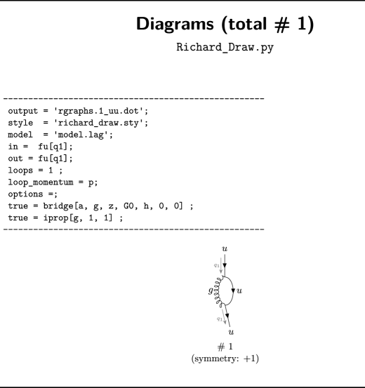
Figure 1: Example of richard_draw output for the problem SM/loop.1_uu.dat.

5 Example

In this section we briefly discuss the calculation of the divergent part of the QCD quark self energy, in order to illustrate the usage of MaRTIn. This example uses the following files that are distributed together with the code: The Standard Model FORM-model file model_SM, located in user_template/models/form, the Standard Model qgraf-model files standardmodel.prop.lag and standardmodel.vrtx.lag, located in user_template/models/qgraf, and the problem file loop.1_uu.dat located in user_template/problems/SM. The latter is calling the dolour procedure from the base code to simplify the colour structure. This example should give a good illustration of how to read the output of MaRTIn.

The corresponding call of MaRTIn, e.g., from the user_template directory, would be:

⬇

martin problems/SM/loop.1_uu.dat

which would generate and compute all diagrams. In this example there is a single diagram, see Fig. 1.

This will result in a screen printout, which includes the following lines:

⬇

-----------------------------------------------------------------------

Massive Recursive Tensor Integration

M a R T I n

Copyright (C) 2009-2023 J. Brod, L. Huedepohl, E. Stamou, T. Steudtner

MaRTIn is licensed under the GNU General Public License Version 3.

-----------------------------------------------------------------------

Extracted default configuration from config file: "~/.martin.conf"

Computing using the input of the loop.dat:

xxx/user_template/problems/SM/loop.1_uu.dat

The problem suffix of the loop.dat is:

suffix = ".1_uu"

The problem directory is:

xxx/user_template/problems/SM

The results directory is:

[inferred from loop.dat] : xxx/user_template/results/SM

The user_prc directories are (in order of importance):

[inferred from loop.dat] : xxx/user_template/prc

The FORM models are:

[inferred from loop.dat] : xxx/user_template/models/form/model_SM

The QGRAF models are:

[inferred from loop.dat] : xxx/user_template/models/qgraf/sm.prop.lag

[inferred from loop.dat] : xxx/user_template/models/qgraf/sm.vrtx.lag

The JSON files for richard_draw.py are:

[inferred from loop.dat] : xxx/user_template/models/rdraw/standardmodel.json

Computing based on GIT commit: "<hash>" (Modulo local/uncommited modifications)

These lines just explicitly list the files used by MaRTIn in that particular run. (In practice, xxx will correspond to the base directory that is actually used.) The git commit version is also indicated. This is followed by information on the generation of the diagrams:

⬇

Running "make"...

Generating xxx/user_template/results/SM/qgraf.1_uu.dat ...

Generating xxx/user_template/results/SM/qlist.1_uu.dat ...

Running QGRAF ...

-------------------------------------------------------

qgraf-3.1.4

-------------------------------------------------------

output = ’qlist.1_uu.dat’;

style = ’main.sty’;

model = ’model.lag’;

in = fu[q1];

out = fu[q1];

loops = 1 ;

loop_momentum = p;

options =;

true = bridge[a, g, z, G0, h, 0, 0] ;

true = iprop[g, 1, 1] ;

-------------------------------------------------------

24P --- 7+ 17- --- 5N+ 2C+ 17C-

163V --- 3^136 4^27

-------------------------------------------------------

- 4^1 --- 0 diagrams

3^2 - --- 1 diagram

total = 1 diagram

Generating xxx/user_template/results/SM/make.1_uu.info ...

rm xxx/user_template/results/SM/qlist.1_uu.dat

Generating xxx/user_template/results/SM/qgraf.1_uu.dat ...

Generating xxx/user_template/results/SM/form.1_uu.dat ...

Finally, FORM is invoked to perform the actual calculation:

⬇

Computing xxx/user_template/results/SM/form.1_uu/dia1.sav ...

FORM 4.2.1 (Feb 6 2019, v4.2.1-3-g558b01f) 64-bits Run: <date and time>

#-

dia1 =

+ ep^-1 * (

- 3/4*UbarSp(fu,su3col,j1,mom,q1)*DIRAC(1,one)*USp(fu,su3col,j1,mom,

q1)*i_*pi^-1*alphas*Mup*CF

- 1/4*UbarSp(fu,su3col,j1,mom,q1)*DIRAC(1,one)*USp(fu,su3col,j1,mom,

q1)*i_*pi^-1*xiqg*alphas*Mup*CF

+ 1/4*UbarSp(fu,su3col,j1,mom,q1)*DIRAC(1,q1)*USp(fu,su3col,j1,mom,

q1)*i_*pi^-1*xiqg*alphas*CF

);

0.10 sec out of 0.10 sec

Done computing xxx/user_template/results/SM/form.1_uu/dia1.sav.

MaRTIn finished.

The following code in the FORM folds in the problem file has been used to simplify the output

⬇

*--#[ USERDEF :

s CF,alphas;

*--#] USERDEF :

*--#[ FOLD1 :

#include docolour

*--#] FOLD1 :

*--#[ FOLD5 :

id eM(mIRA) = 1;

id nc = 2*CF + 1/nc;

id gs^2 = 4*pi*alphas;

*--#] FOLD5 :

This is used to replace eM(mIRA) by $1$ and gs by $\sqrt{4\pi\alpha_{s}}$, as well as powers of $N_{c}$ in terms of $C_{F}\equiv(N_{c}^{2}-1)/2N_{c}$. Note that the spinorial objects UbarSp, DIRAC, and USp are non-commuting. The final output then corresponds to the familiar expression

$$\texttt{dia1}=-\frac{i\alpha_{s}}{4\pi}C_{F}\frac{1}{\varepsilon}\bar{u}(\boldsymbol{q}_{1},j_{1})\Big{[}\xi_{G}\not{q}_{1}+m_{u}(3+\xi_{G})\Big{]}u(\boldsymbol{q}_{1},j_{1})\,.$$ (4)

The result is saved as dia1.sav in the directory user_template/results/SM/form.1_uu and can be loaded using FORM’s load command. A Mathematica-readable (text-)file dia1.m is saved in the directory user_template/results/SM/math.1_uu. Its contents are

⬇

(* dia1 *) { - 3/4*MathDirac[UbarSp[fu,su3col,j1,mom,q1],USp[fu,su3col,

j1,mom,q1]]*I*Pi^(-1)*ep^(-1)*alphas*Mup*CF - 1/4*MathDirac[

UbarSp[fu,su3col,j1,mom,q1],USp[fu,su3col,j1,mom,q1]]*I*Pi^(-1)*

ep^(-1)*xiqg*alphas*Mup*CF + 1/4*MathDirac[UbarSp[fu,su3col,j1,

mom,q1],q1,USp[fu,su3col,j1,mom,q1]]*I*Pi^(-1)*ep^(-1)*xiqg*

alphas*CF}

Acknowledgements

We would like to thank Martin Gorbahn for many cross checks of our code during various fruitful collaborations. J.B. acknowledges support in part by DoE grant DE-SC1019775.

Appendix A Implementation of four-fermion vertices

QGRAF does not allow for the generation of local four-fermion vertices. They can, however, be implemented in a straightforward way using auxiliary propagators. The following example shows how to implement the four-quark operator $Q=(\bar{s}_{L}\gamma^{\mu}c_{L})(\bar{u}_{L}\gamma_{\mu}d_{L})$. Here, $q_{L}\equiv\tfrac{1}{2}(1-\gamma_{5})q$ denote the left-handed quark fields ($q=u,d,s,c$).

The QGRAF model file should include

⬇

*   Artificial propagator:

[sp,sm,+;pfunct=’Dmu’,m=’M0’]

*   Vertices for the two quark bilinears:

[fS,fc,sp;vfunct=’FSc’]

[fU,fd,sm;vfunct=’FUd’]

We assume that all functions and symbols have been properly declared, and color indices have been generated. The vertex can then be substituted in two steps. If vertex symbols vFSc and vFUd (together with the corresponding vertex functions FSc and FUd) have been defined and included in the FF and VERTICES folds, we include the following substitution rule in the INSERTFERMIONVERTICES fold:

⬇

*--#[ INSERTFERMIONVERTICES :

*

id FL‘i’(?a,vFUd,lorentz,mu1?,mom,q1?,q2?,q3?)

= FL‘i’(?a)*g_(‘i’,mu1)*PL‘i’;

id FL‘i’(?a,vFSc,lorentz,mu1?,mom,q1?,q2?,q3?)

= FL‘i’(?a)*g_(‘i’,mu1)*PL‘i’;

*

*--#] INSERTFERMIONVERTICES :

Here, we made use of the unique Lorentz indices that have been generated automatically for the artificial “propagator field”. (This trick does not work for operators with longer strings of Dirac matrices, in which case the Lorentz indices have to be inserted/generated “by hand”.) Finally, we use the substitution of the artificial propagator to contract the correct pairs of Lorentz indices, by simply replacing it by a metric tensor:

⬇

*--#[ INSERTPROPAGATORS :

*

id Dmu(xx1?,xx2?,lorentz,mu1?,mu2?,mom,?p,mass,M?,field,fname?)

= d_(mu1,mu2) ;

*

*--#] INSERTPROPAGATORS :

Note that gengraph will automatically supply a factor vFSc*vFUd, which can then be substituted by the Wilson coefficient of the operator. For instance, if the Lagrangian in the current example is ${\mathcal{L}}=\sqrt{2}G_{F}CQ$, one would include the following substitution rule in the INSERTCOUPLINGS fold:

⬇

*--#[ INSERTCOUPLINGS :

id vFSc*vFUd = i_*sqrt_(2)*GF*C ;

*--#] INSERTCOUPLINGS :

References

- [1] P. Nogueira. “Automatic Feynman graph generation”. J. Comput. Phys. 105:279, 1993. 10.1006/jcph.1993.1074.
- [2] T. Hahn and M. Perez-Victoria. “Automatized one loop calculations in four-dimensions and D-dimensions”. Comput. Phys. Commun. 118:153, 1999. 10.1016/S0010-4655(98)00173-8. hep-ph/9807565.
- [3] T. Hahn. “Generating Feynman diagrams and amplitudes with FeynArts 3”. Comput. Phys. Commun. 140:418, 2001. 10.1016/S0010-4655(01)00290-9. hep-ph/0012260.
- [4] J. A. M. Vermaseren. “New features of FORM” 2000. math-ph/0010025.
- [5] J. Kuipers, T. Ueda, J. A. M. Vermaseren and J. Vollinga. “FORM version 4.0”. Comput. Phys. Commun. 184:1453, 2013. 10.1016/j.cpc.2012.12.028. 1203.6543.
- [6] M. Tentyukov and J. Fleischer. “A Feynman diagram analyzer DIANA”. Comput. Phys. Commun. 132:124, 2000. 10.1016/S0010-4655(00)00147-8. hep-ph/9904258.
- [7] R. Harlander, T. Seidensticker and M. Steinhauser. “Complete corrections of Order alpha alpha-s to the decay of the Z boson into bottom quarks”. Phys. Lett. B 426:125, 1998. 10.1016/S0370-2693(98)00220-2. hep-ph/9712228.
- [8] T. Seidensticker. “Automatic application of successive asymptotic expansions of Feynman diagrams”. In “6th International Workshop on New Computing Techniques in Physics Research: Software Engineering, Artificial Intelligence Neural Nets, Genetic Algorithms, Symbolic Algebra, Automatic Calculation”, 1999. hep-ph/9905298.
- [9] F. Herren. Precision Calculations for Higgs Boson Physics at the LHC - Four-Loop Corrections to Gluon-Fusion Processes and Higgs Boson Pair-Production at NNLO. Ph.D. thesis, KIT, Karlsruhe, 2020. 10.5445/IR/1000125521.
- [10] M. Gerlach, F. Herren and M. Lang. “tapir: A tool for topologies, amplitudes, partial fraction decomposition and input for reductions”. Comput. Phys. Commun. 282:108544, 2023. 10.1016/j.cpc.2022.108544. 2201.05618.
- [11] J. Hoff. “The Mathematica package TopoID and its application to the Higgs boson production cross section”. J. Phys. Conf. Ser. 762(1):012061, 2016. 10.1088/1742-6596/762/1/012061. 1607.04465.
- [12] Margerya, V. “Alibrary”. https://github.com/magv/alibrary 2021.
- [13] Margerya, V. “Feynson”. https://github.com/magv/feynson 2020.
- [14] G. Passarino and M. J. G. Veltman. “One Loop Corrections for e+ e- Annihilation Into mu+ mu- in the Weinberg Model”. Nucl. Phys. B 160:151, 1979. 10.1016/0550-3213(79)90234-7.
- [15] R. N. Lee. “Presenting LiteRed: a tool for the Loop InTEgrals REDuction” 2012. 1212.2685.
- [16] R. N. Lee. “LiteRed 1.4: a powerful tool for reduction of multiloop integrals”. J. Phys. Conf. Ser. 523:012059, 2014. 10.1088/1742-6596/523/1/012059. 1310.1145.
- [17] A. V. Smirnov. “Algorithm FIRE – Feynman Integral REduction”. JHEP 10:107, 2008. 10.1088/1126-6708/2008/10/107. 0807.3243.
- [18] A. V. Smirnov and V. A. Smirnov. “FIRE4, LiteRed and accompanying tools to solve integration by parts relations”. Comput. Phys. Commun. 184:2820, 2013. 10.1016/j.cpc.2013.06.016. 1302.5885.
- [19] A. V. Smirnov. “FIRE5: a C++ implementation of Feynman Integral REduction”. Comput. Phys. Commun. 189:182, 2015. 10.1016/j.cpc.2014.11.024. 1408.2372.
- [20] A. V. Smirnov and F. S. Chuharev. “FIRE6: Feynman Integral REduction with Modular Arithmetic”. Comput. Phys. Commun. 247:106877, 2020. 10.1016/j.cpc.2019.106877. 1901.07808.
- [21] C. Studerus. “Reduze-Feynman Integral Reduction in C++”. Comput. Phys. Commun. 181:1293, 2010. 10.1016/j.cpc.2010.03.012. 0912.2546.
- [22] A. von Manteuffel and C. Studerus. “Reduze 2 - Distributed Feynman Integral Reduction” 2012. 1201.4330.
- [23] P. Maierhöfer, J. Usovitsch and P. Uwer. “Kira—A Feynman integral reduction program”. Comput. Phys. Commun. 230:99, 2018. 10.1016/j.cpc.2018.04.012. 1705.05610.
- [24] J. Klappert, F. Lange, P. Maierhöfer and J. Usovitsch. “Integral reduction with Kira 2.0 and finite field methods”. Comput. Phys. Commun. 266:108024, 2021. 10.1016/j.cpc.2021.108024. 2008.06494.
- [25] S. A. Larin, F. V. Tkachov and J. A. M. Vermaseren. “The FORM version of MINCER” 1991.
- [26] M. Steinhauser. “MATAD: A Program package for the computation of MAssive TADpoles”. Comput. Phys. Commun. 134:335, 2001. 10.1016/S0010-4655(00)00204-6. hep-ph/0009029.
- [27] B. Ruijl, T. Ueda and J. A. M. Vermaseren. “Forcer, a FORM program for the parametric reduction of four-loop massless propagator diagrams”. Comput. Phys. Commun. 253:107198, 2020. 10.1016/j.cpc.2020.107198. 1704.06650.
- [28] A. Pikelner. “FMFT: Fully Massive Four-loop Tadpoles”. Comput. Phys. Commun. 224:282, 2018. 10.1016/j.cpc.2017.11.017. 1707.01710.
- [29] M. Misiak and M. Munz. “Two loop mixing of dimension five flavor changing operators”. Phys. Lett. B 344:308, 1995. 10.1016/0370-2693(94)01553-O. hep-ph/9409454.
- [30] K. G. Chetyrkin, M. Misiak and M. Munz. “Beta functions and anomalous dimensions up to three loops”. Nucl.Phys. B518:473, 1998. 10.1016/S0550-3213(98)00122-9. hep-ph/9711266.
- [31] A. I. Davydychev and J. Tausk. “Two loop selfenergy diagrams with different masses and the momentum expansion”. Nucl.Phys. B397:123, 1993. 10.1016/0550-3213(93)90338-P.
- [32] C. Bobeth, M. Misiak and J. Urban. “Photonic penguins at two loops and m(t) dependence of BR[B X(s) lepton+ lepton-]”. Nucl.Phys. B574:291, 2000. 10.1016/S0550-3213(00)00007-9. hep-ph/9910220.
- [33] Wolfram Research, Inc. “Mathematica, Version 13.2”. https://www.wolfram.com/mathematica Champaign, IL, 2022.
- [34] Free Software Foundation. “GNU General Public License, Version 3”. http://www.gnu.org/licenses/gpl.html June 29th, 2007.
- [35] F. Jegerlehner. “Facts of life with gamma(5)”. Eur. Phys. J. C 18:673, 2001. 10.1007/s100520100573. hep-th/0005255.
- [36] J. C. Collins. Renormalization: An Introduction to Renormalization, The Renormalization Group, and the Operator Product Expansion, volume 26 of Cambridge Monographs on Mathematical Physics. Cambridge University Press, Cambridge, 1986. ISBN 978-0-521-31177-9, 978-0-511-86739-2. 10.1017/CBO9780511622656.
- [37] K. G. Chetyrkin and M. F. Zoller. “Three-loop \beta-functions for top-Yukawa and the Higgs self-interaction in the Standard Model”. JHEP 06:033, 2012. 10.1007/JHEP06(2012)033. 1205.2892.
- [38] A. V. Bednyakov, A. F. Pikelner and V. N. Velizhanin. “Yukawa coupling beta-functions in the Standard Model at three loops”. Phys. Lett. B 722:336, 2013. 10.1016/j.physletb.2013.04.038. 1212.6829.
- [39] G. ’t Hooft and M. J. G. Veltman. “Regularization and Renormalization of Gauge Fields”. Nucl. Phys. B 44:189, 1972. 10.1016/0550-3213(72)90279-9.
- [40] P. Breitenlohner and D. Maison. “Dimensionally Renormalized Green’s Functions for Theories with Massless Particles. 1.” Commun. Math. Phys. 52:39, 1977. 10.1007/BF01609070.
- [41] P. Breitenlohner and D. Maison. “Dimensionally Renormalized Green’s Functions for Theories with Massless Particles. 2.” Commun. Math. Phys. 52:55, 1977. 10.1007/BF01609071.
- [42] P. Breitenlohner and D. Maison. “Dimensional Renormalization and the Action Principle”. Commun. Math. Phys. 52:11, 1977. 10.1007/BF01609069.
- [43] S. A. Larin. “The Renormalization of the axial anomaly in dimensional regularization”. Phys. Lett. B 303:113, 1993. 10.1016/0370-2693(93)90053-K. hep-ph/9302240.