Dynamics Near the Inner Dead-Zone Edges in a Proprotoplanetary Disk

Abstract

We perform three-dimensional global non-ideal magnetohydrodynamic simulations of a protoplanetary disk containing the inner dead-zone edge. We take into account realistic diffusion coefficients of the Ohmic resistivity and ambipolar diffusion based on detailed chemical reactions with a single-size dust grains. We found that the conventional dead zone identified by the Elsässer numbers of the Ohmic resistivity and ambipolar diffusion is divided into two regions: ”the transition zone” and ”the coherent zone”. The coherent zone has the same properties as the conventional dead zone, and extends outside of the transition zone in the radial direction. Between the active and coherent zones, we discover the transition zone whose inner edge is identical to that of the conventional dead-zone. The transition zone extends out over the regions where thermal ionization determines diffusion coefficients. The transition zone has completely different physical properties than the conventional dead zone, the so-called undead zone, and zombie zone. Combination of amplification of the radial magnetic field owing to the ambipolar diffusion and a steep radial gradient of the Ohmic diffusivity causes the efficient evacuation of the net vertical magnetic flux from the transition zone within several rotations. Surface gas accretion occurs in the coherent zone but not in the transition zone. The presence of the transition zone prohibits mass and magnetic flux transport from the coherent zone to the active zone. Mass accumulation occurs at both edges of the transition zone as a result of mass supply from the active and coherent zones.

1 Introduction

The evolution of protoplanetary disks (PPDs) is controlled by angular momentum transfer. One of the important angular momentum transfer mechanisms is the magnetorotational instability (MRI, Velikhov, 1959; Chandrasekhar, 1961; Balbus & Hawley, 1991). The turbulence driven by MRI transfers angular momentum radially. MRI has been extensively investigated in local shearing-box simulations (e.g., Hawley et al., 1995) and in global simulations (Armitage, 1998; Hawley et al., 2011; Sorathia et al., 2012; Suzuki & Inutsuka, 2014; Takasao et al., 2018; Zhu & Stone, 2018; Jacquemin-Ide et al., 2021).

Low ionization degrees in PPDs induce the non-ideal MHD effects and affect the growth of the MRI. There are three non-ideal MHD effects, Ohmic resistivity (OR), Hall effect (HE), and ambipolar diffusion (AD). The regions where non-ideal MHD effects suppress the MRI are called dead zones (Gammie, 1996). Ionization fractions sufficient to drive the MRI are provided only in innermost and outermost radii and upper atmosphere of PPDs owing to thermal ionization, far-ultraviolet and X-ray radiation from the central star, and cosmic rays.

The angular momentum transfer in the inner regions ($R\lesssim 10~{}$au) of PPDs where OR plays an important role was investigated in Gammie (1996). He showed that so-called layered accretion is driven around the disk surfaces where MRI is active while the MRI is completely suppressed in the disk interior. Detailed linear analyses of the MRI modified by OR were done by Jin (1996) and Sano & Miyama (1999). MRI-driven turbulence above the dead zone was also studied in local simulations (Fleming & Stone, 2003; Turner & Sano, 2008; Hirose & Turner, 2011)

When AD operates in addition to OR, the MRI is suppressed even in the disk surface and the layered accretion disappears because AD works in higher latitudes than OR (Bai & Stone, 2013). Instead of the layered accretion, the $\phi z$ component of the magnetic stress owing to global coherent magnetic fields drives laminar surface gas accretion just above the dead zone in the inner region of PPDs where both OR and AD are important (Bai & Stone, 2013; Bai, 2013; Gressel et al., 2015).

The inner dead-zone edge, inside which the thermal ionization activates the MRI, has attracted attention as a dust accumulation site. In such a region, a local pressure bump is created because the outer part of the active zone moves outward owing to a negative turbulent viscosity gradient. A pressure bump at the inner dead-zone edge traps dust particles in the dead zone that are moving to the pressure bump (Kretke et al., 2009; Ueda et al., 2019).

The inner dead-zone edge has been investigated with global simulations taking OR into account. Dzyurkevich et al. (2010) found that a pressure bump develops at the inner dead-zone edge. Lyra & Mac Low (2012) pointed out that the Rossby-wave instability (Lovelace et al., 1999) induces the formation of vortices at the pressure bump. Flock et al. (2017) performed realistic non-ideal MHD simulations with radiation transfer, and found that a vortex forms at the inner dead-zone edge that casts a nonaxisymmetric shadow on the outer disk.

In the global simulations containing the inner dead-zone edge performed by Dzyurkevich et al. (2010) and Lyra & Mac Low (2012), the angular momentum of the disk is transferred by the MRI turbulence above the dead zone (Gammie, 1996). They observed that the height-averaged mass accretion stress does not change significantly across the dead-zone edge. Although sudden decreases in the accretion stresses are found across the inner dead-zone edge in Flock et al. (2017), their range of the polar angle may not be wide enough for the MRI to occur above the dead zone. In addition, in their simulations, the spatial distributions of the OR coefficient are given by simplified analytic formulae with a sharp transition across the inner dead-zone edge.

Inclusion of AD changes the angular momentum transfer mechanism in the dead zone from the MRI turbulence. The MRI above the dead zone will be suppressed once AD is considered (Bai & Stone, 2013; Gressel et al., 2015; Bai, 2017). In a realistic situation where both OR and AD work, the angular momentum transfer mechanism changes from the MRI turbulence to the magnetic stress due to global coherent magnetic field across the inner dead-zone edge. When both OR and AD are considered, the spatial distribution of the accretion stress across the inner dead-zone edge is still unclear.

In this paper, we perform global three-dimensional non-ideal MHD simulations of a protoplanetary disk around an intermediate mass star to reveal the structure around the inner dead-zone edge by taking into account both OR and AD whose coefficients are given based on detailed chemistry. In the previous global simulations, a limited range of $\theta$ in the spherical polar coordinates of $(r,\theta,\phi)$ is considered, which may affect surface gas accretion expected to be driven above the dead zone (Bai & Stone, 2013) and launching of disk winds both from the active zone (Suzuki & Inutsuka, 2009, 2014) and the dead zone (Bai & Stone, 2013). Our simulation box covers a full solid angle ($0\leq\theta\leq\pi$ and $0\leq\phi<2\pi$) to capture the angular momentum transfer in the upper atmosphere and vortex formation.

This paper is organized as follows. We will describe the numerical setup and method in Section 2. The main results are presented in Section 3. In Section 4, we will present detailed analyses on transfer of the mass, angular momentum, and magnetic flux in the disk. Astrophysical implications are discussed in Section 5. Our findings are summarized in Section 6.

2 Numerical Setup and Methods

2.1 Basic Equations

The resistive MHD equations with OR and AD are given by

$$\frac{\partial\rho}{\partial t}+\bm{\nabla}\cdot\left(\rho\bm{v}\right)=0$$ (1)

$$\frac{\partial\rho\bm{v}}{\partial t}+\bm{\nabla}\cdot\left(\rho\bm{v}\otimes\bm{v}+{\bf T}\right)=-\rho\bm{\nabla}\phi,$$ (2)

$$\frac{\partial\bm{B}}{\partial t}=\mathbf{\nabla}\times\left(\bm{v}\times\bm{B}\right)-\mathbf{\nabla}\times\left[\eta_{\mathrm{O}}\bm{J}+\eta_{\mathrm{A}}\bm{J}_{\perp}\right]$$ (3)

and

$${\bf T}=\left(P+\frac{B^{2}}{8\pi}\right){\bf I}-\frac{\bm{B}\otimes\bm{B}}{4\pi},$$ (4)

where $\rho$ is the gas density, $\bm{v}$ is the gas velocity, $\bm{B}$ is the magnetic field, $\phi$ is the gravitational potential of the central star, $\bm{J}$ is the current density, $\bm{J}_{\perp}\equiv\bm{J}-\bm{J}\cdot\bm{B}/|\bm{B}|$ is the electric current density perpendicular to the local magnetic field, $P$ is the gas pressure, ${\bf T}$ is the stress tensor, ${\bf I}$ is the identity matrix, $\eta_{\mathrm{O}}$ and $\eta_{\mathrm{A}}$ are the diffusion coefficients for OR and AD, respectively. They are defined in Section 2.2.2. For simplicity, the Hall effect is neglected in this work.

In this paper, for simplicity we use the locally isothermal equation of state where the gas temperature remains the same as the initial one (Suzuki & Inutsuka, 2014; Zhu & Stone, 2018). To achieve this, we solve the MHD equations including the energy equation with $\gamma=5/3$, and the gas pressure is derived from the locally isothermal condition where the temperature distribution is shown in Equation (10). We note that a locally isothermal equation of state potentially drives the vertical shear instability (VSI) (Nelson et al., 2013). In the active zone, Latter & Papaloizou (2018) shows that the VSI is suppressed by magnetic fields in the ideal MHD limit (also see Cui & Lin, 2021; Latter & Kunz, 2022). In the dead-zone, OR can revive the VSI if the Elässer number is sufficiently low. Latter & Kunz (2022) show that the behaviours of AD are rather complicated because the VSI is coupled with AD shear-instability (Kunz, 2008). In our simulations, at least in the regions around the inner dead-zone edge, which is focused on in this paper, the VSI does not appear to grow because the gas is significantly disturbed by the MRI turbulence in the active zone. The radial velocity dispersion is much larger than the vertical one, which is not expected in the VSI growth mode. By contrast, outer regions far from the inner dead-zone edge can suffer from the VSI. Our simulation time however is too short to see the growth the VSI in such outer regions.

2.2 Models and Methods

2.2.1 Initial Condition

The initial surface density profile of the disk is given by

$$\Sigma_{\mathrm{ini}}(R)=\Sigma_{0}\left(\frac{R}{1~{}\mathrm{au}}\right)^{-1}$$ (5)

where $\Sigma_{0}=500~{}\mathrm{g~{}cm^{-2}}$ and $R$ is the cylindrical radius. The disk mass integrated from $R=0$ to $R$ is given by

$$M_{\mathrm{d}}(R)=2.35\times 10^{-4}~{}M_{\odot}~{}\left(\frac{\Sigma_{0}}{500~{}\mathrm{g~{}cm^{-2}}}\right)\left(\frac{R}{1~{}\mathrm{au}}\right)^{1.5}.$$ (6)

The mid-plane gas temperature $T_{\mathrm{mid}}$ is determined by assuming radiative equilibrium between the gas and radiation from the central star. We consider a central star with $M_{*}=2.5~{}M_{\odot}$ of mass, $R_{*}=2.5~{}R_{\odot}$ of radius, and $T_{*}=10^{4}~{}\mathrm{K}$ of effective temperature, which corresponds to a Herbig Ae star. The mid-plane gas temperature is given by

$$T_{\mathrm{mid}}(R)=760~{}\mathrm{K}~{}f_{\mathrm{boost}}\left(\frac{L_{*}}{56L_{\odot}}\right)^{1/4}\left(\frac{R}{1~{}\mathrm{au}}\right)^{-1/2},$$ (7)

where $f_{\mathrm{boost}}$ is a coefficient which is set to 2 to increase the aspect ratio of the disk, $L_{*}=4\pi R_{*}^{2}\sigma_{\mathrm{SB}}T_{*}^{4}$ is the luminosity of the central star, and $\sigma_{\mathrm{SB}}$ is the Stefan-Boltzmann constant. The adopted stellar luminosity is typical in Herbig Ae stars with ages larger than 1 Myr although the luminosities of Herbig Ae stars with ages less than 1 Myr are highly uncertain (e.g., Montesinos et al., 2009). The scale height is given by $H(R)=\sqrt{2}c_{\mathrm{s,mid}}/\Omega_{\mathrm{K}}(R)$, where $c_{\mathrm{s,mid}}=\sqrt{k_{\mathrm{B}}T_{\mathrm{mid}}/\mu m_{\mathrm{H}}}$ is the sound speed at the mid-plane, $\mu=2.33$ is the mean molecular weight, $m_{\mathrm{H}}$ is the hydrogen mass, and $\Omega_{\mathrm{K}}=\sqrt{GM_{*}/R^{3}}$ is the Kepler angular velocity of the disk. The aspect ratio of the disk is given by

$$\epsilon_{\mathrm{mid}}(R)=\frac{H(R)}{R}=0.049f_{\mathrm{boost}}^{1/2}\left(\frac{R}{1~{}\mathrm{au}}\right)^{1/4},$$ (8)

The initial mid-plane density is given by

$$\rho_{\mathrm{mid,ini}}(R) = 5.4\times 10^{-10}~{}\mathrm{g~{}cm^{-3}}$$ (9)

$$\times f_{\mathrm{boost}}^{-1/2}\left(\frac{\Sigma_{0}}{500~{}\mathrm{g~{}cm^{-2}}}\right)\left(\frac{r}{1~{}\mathrm{au}}\right)^{-9/4}.$$

We consider a similar temperature distribution as Bai (2017). The whole region is divided into a cold gas disk and warm atmospheres sandwiching the cold disk. Inside the disk, the temperature is given by $T_{\mathrm{d}}(r)=(\mu m_{\mathrm{H}}/k_{\mathrm{B}})(\epsilon_{\mathrm{mid}}(r)^{2}/2)r^{2}\Omega_{\mathrm{K}}(r)^{2}$ which is identical to $T_{\mathrm{mid}}$ (Equation (7)) at the mid-plane. In the warm atmosphere well above the disk, the gas is heated up mainly by the radiation from the central star. We define $\Sigma_{\mathrm{FUV}}$ as the column density below which the FUV photons from the central star penetrate. If the radial column density $\Sigma_{r}(r,\theta)=\int_{r_{\mathrm{min}}}^{r}\rho(r^{\prime},\theta)dr^{\prime}$ is smaller than $\Sigma_{\mathrm{FUV}}$, the gas temperature increases to $T_{\mathrm{atm}}(r)=(\mu m_{\mathrm{H}}/k_{\mathrm{B}})(\epsilon_{\mathrm{atm}}(r)^{2}/2)r^{2}\Omega_{\mathrm{K}}(r)^{2}$, where $\epsilon_{\mathrm{atm}}(r)=0.2(r/1~{}\mathrm{au})^{1/4}$. The initial temperature profile smoothly connects between $T_{\mathrm{d}}$ and $T_{\mathrm{atm}}$ around $\Sigma_{r}\sim\Sigma_{\mathrm{FUV}}$ as follows:

$$T(r,\theta)=(\mu m_{\mathrm{H}}/k_{\mathrm{B}})(\epsilon(r)^{2}/2)r^{2}\Omega_{\mathrm{K}}(r)^{2}$$ (10)

and

$$\epsilon(r,\theta) = \frac{\epsilon_{\mathrm{mid}}(r)+\epsilon_{\mathrm{atm}}(r)}{2}$$ (11)

$$+ \frac{\epsilon_{\mathrm{mid}}(r)-\epsilon_{\mathrm{atm}}(r)}{2}\tanh\left[0.3\log\left(\frac{\Sigma_{\mathrm{FUV}}}{\Sigma_{r}(r,\theta)}\right)\right].$$

The values of $\Sigma_{\mathrm{FUV}}$ are highly uncertain, and Perez-Becker & Chiang (2011) found that FUV layers have a thickness of $\sim 0.01-0.1$ g cm^-2 in plane-parallel models. We adopt $\Sigma_{\mathrm{FUV}}=0.3~{}\mathrm{g~{}cm^{-2}}$. It is three times larger than the upper limit of that of Perez-Becker & Chiang (2011) because the radial column density is considered instead of the vertical column density (Bai, 2017).

The aspect ratio for $R<1~{}$au is too small to resolve the MRI structure. As explained below Equation (7), we artificially increase the aspect ratio by increasing the gas temperature by a factor of two, or $f_{\mathrm{boost}}=2$. As mentioned later, for the calculation of $\eta_{\mathrm{O}}$ and $\eta_{\mathrm{A}}$, $Tf_{\mathrm{boost}}^{-1}$ is used as the gas temperature.

The initial profiles of the density and $\phi$ component of the velocity are constructed using an iterative manner to satisfy equations (5) and (10) simultaneously in the hydrostatic equilibrium between the pressure-gradient force, gravitational force, and centrifugal force without the Lorentz force. The initial poloidal velocities are set to be zero. The initial magnetic field has only the poloidal components which have an hourglass-shape field given by Zanni et al. (2007). It is described by the $\phi$ component of the vector potential,

$$A_{\phi}(r,\theta)=Cr^{-a}\left[m^{2}+\left(\frac{z}{r}\right)^{2}\right]^{-5/8},$$ (12)

where the coefficient $C$ is determined so that the mid-plane plasma beta takes a constant value of $\beta_{0}=10^{4}$. The initial condition of our simulation is displayed in Figure 1.

A height of the base of the atmospheres at a given $R$ is denoted by $z=z_{\mathrm{atm}}(R)$ above which the gas temperature is more than twice the mid-plane temperature (Figure 1).

2.2.2 Diffusion Coefficients

The diffusion coefficients $\eta_{\mathrm{O}}$ and $\eta_{\mathrm{A}}$ are given by

$$\eta_{\mathrm{O}}=\frac{c^{2}}{4\pi}\frac{1}{\sigma_{\mathrm{O}}}\;\;\mathrm{and}\;\;\eta_{\mathrm{A}}=\frac{c^{2}}{4\pi}\left(\frac{\sigma_{\mathrm{P}}}{\sigma_{\mathrm{P}}^{2}+\sigma_{\mathrm{H}}^{2}}-\frac{1}{\sigma_{\mathrm{O}}}\right),$$ (13)

where $\sigma_{\mathrm{O}}$, $\sigma_{\mathrm{H}}$, and $\sigma_{\mathrm{P}}$ are the Ohmic, Hall, and Pedersen conductivities, respectively, and $c$ is the speed of light. The three conductivities are given by

$$\sigma_{\mathrm{O}}=\frac{ec}{B}\sum_{j}n_{j}|Z_{j}|\beta_{j},$$ (14)

$$\sigma_{\mathrm{H}}=-\frac{ec}{B}\sum_{j}\frac{n_{j}Z_{j}\beta_{j}^{2}}{1+\beta_{j}^{2}},$$ (15)

and

$$\sigma_{\mathrm{P}}=\frac{ec}{B}\sum_{j}\frac{n_{j}|Z_{j}|\beta_{j}}{1+\beta_{j}^{2}},$$ (16)

where the subscript “$j$” denotes the species of charged particles, $Z_{j}e$ is the charge and $n_{j}$ is the density of the charged particle $j$. The Hall parameter $\beta_{j}$ is the ratio between the gyrofrequency of the charged particle $j$ and its collision frequency with the neutral particles, and is defined as

$$\beta_{j}=\frac{|Z_{j}|eB}{m_{j}c}\frac{1}{\gamma_{j}\rho},$$ (17)

where $m_{j}$ is the mass of the charged particle $j$ and $\gamma_{j}$ is the rate coefficient for momentum transfer with the neutral particles through collisions.

The three conductivities are computed by the summation between the conductivities calculated with thermal and non-thermal ionization instead of calculating a chemical network including both thermal and non-thermal ionization, as follows:

$$\sigma_{i}=\sigma_{i,\mathrm{T}}+\sigma_{i,\mathrm{NT}},$$ (18)

where $i=(\mathrm{O,H,P})$ and the subscripts “T” and “NT” indicate the thermal and non-thermal ionization limits of the conductivities, respectively.

Since the thermal ionization is important in the regions of sufficiently high temperatures, dust grains are assumed to be sublimated in the calculation of chemical reactions. We consider the thermal ionization of potassium, which has an ionization energy of 3.43 eV. The potassium abundance relative to the H₂ number density is $3\times 10^{-7}$. The thermal ionization degree $(x_{e})_{\mathrm{T}}$ is derived by the Saha equation where the electron densities are assumed to be equal to the potassium ion densities. As mentioned before, $T$ is replaced with $Tf_{\mathrm{boost}}^{-1}$ in the Saha equation. When the gas temperature exceeds $\sim 1000~{}$K, the thermal ionization of K provides a sufficient high ionization and the region becomes MRI active.

In order to take into account the photo-ionization of carbon and sulfur due to FUV photons in the disk atmosphere, we replaced the ionization degree calculated in the thermal ionization limit by

$$\max\left[\left(x_{e}\right)_{\mathrm{T}},10^{-4}\exp\left\{-\left(\frac{\Sigma_{r}(r,\theta)}{\Sigma_{\mathrm{FUV}}}\right)^{4}\right\}\right],$$ (19)

where $\left(x_{e}\right)_{\mathrm{T}}$ is the ionization degree obtained from the Saha equation for potassium ionization and the second term indicates that the electrons are provided by photo-ionization of carbon and sulfur when $\Sigma_{r}<\Sigma_{\mathrm{FUV}}$ (Bai, 2017).

For the non-thermal ionization, we use the data table of the three conductivities based on a chemical reaction network of e^-, H⁺, He⁺, C⁺, H${}_{3}^{+}$, HCO⁺, Mg⁺ in the gas phase and the charged dust grains using the methods described by Nakano et al. (2002) and Okuzumi (2009). The table is a function of $\rho/B$, $T$, and $\rho/\zeta$, where $\zeta$ is the ionization rate that will be defined in Equation (20) and $T$ is replaced with $Tf_{\mathrm{boost}}^{-1}$. For simplicity, the single size dust grain with a radius of $a=0.1~{}\mu$m and an internal density of $2~{}\mathrm{g~{}cm^{-3}}$ is considered. In this paper, the dust-to-gas mass ratio is set to $10^{-4}$, assuming that dust growth reduces the amount of dust grains smaller than the interstellar value $\sim 0.01$. The following three kinds of non-thermal ionization sources are taken into account,

$$\zeta(r,\theta)=\zeta_{\mathrm{CR}}(r,\theta)+\zeta_{\mathrm{X}}(r,\theta)+\zeta_{\mathrm{radio}}.$$ (20)

The first source is the cosmic rays whose ionization rate is given by

$$\zeta_{\mathrm{CR}}=10^{-17}~{}\mathrm{s}^{-1}\left[\exp\left(-\frac{\Sigma_{\theta}^{+}}{\Sigma_{\mathrm{CR}}}\right)+\exp\left(-\frac{\Sigma_{\theta}^{-}}{\Sigma_{\mathrm{CR}}}\right)\right],$$ (21)

where $\Sigma_{\mathrm{CR}}=96~{}$g cm^-2 (Umebayashi & Nakano, 1981), and $\Sigma_{\theta}^{+}(r,\theta)$ ($\Sigma_{\theta}^{-}(r,\theta)$) is the column density integrated along the $\theta$-direction from $\theta=0$ ($\theta=\pi$) to $\theta$ at a given $r$. Secondly, we consider ionization due to the X-ray radiation from the central star using the fitting formula (Bai & Goodman, 2009, based on the calculation done by Igea & Glassgold (1999)) as follows:

$$\zeta_{\mathrm{X}} = \left(\frac{r}{2.2~{}\mathrm{au}}\right)^{-2.2}\left[\zeta_{1}e^{-(\Sigma_{r}/5\Sigma_{\mathrm{X,a}})^{\alpha}}+\right.$$ (22)

$$\hskip 28.45274pt\left.\zeta_{2}\left\{e^{-(\Sigma_{\theta}^{+}/\Sigma_{\mathrm{X,s}})^{\beta}}+e^{-(\Sigma_{\theta}^{-}/\Sigma_{\mathrm{X,s}})^{\beta}}\right\}\right],$$

where $\zeta_{1}=6.0\times 10^{-11}$ s^-1, $\Sigma_{\mathrm{X,a}}=3.6\times 10^{-3}$ g cm^-2, $\alpha=0.4$, and $\Sigma_{r}(\theta,r)$ is the column density integrated along the $r$-direction from the innermost radius of the simulation box to $r$ at a given $\theta$. The third ionization source is provided by radioactive nuclei,

$$\zeta_{\mathrm{radio}}=6.0\times 10^{-19}~{}\mathrm{s}^{-1}$$ (23)

(Finocchi & Gail, 1997). To reduce the computational cost, $\zeta(r,\theta)$ is calculated for the initial condition and fixed during the simulations.

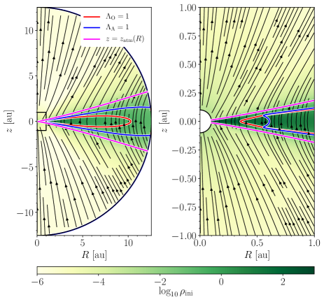
Figure 1: (Left) Initial setup of the simulation. The color map indicates the initial density profile in the code units, and the black lines indicate the streamlines of the magnetic fields. The red (blue) line corresponds to the condition $\Lambda_{\mathrm{O}}=1$ ($\Lambda_{\mathrm{A}}=1$), which show the OR (AD) dead zone boundary. The magenta lines show $z=\pm z_{\mathrm{atm}}(R)$ above which the warm atmospheres exist. The right panel is the same as the left panel but it shows the zoom-in of the region enclosed by the black rectangle shown in the left panel.

2.3 Basic Properties of the Diffusion Coefficients

2.3.1 Definition of the Dead Zone Boundaries

The non-ideal MHD effects affect the growth rate of the MRI when the dimensionless Elsässer numbers

$$\Lambda_{\mathrm{O}}\equiv\frac{v_{\mathrm{A}}^{2}}{\eta_{\mathrm{O}}\Omega_{\mathrm{K}}},\;\;\;\Lambda_{\mathrm{A}}\equiv\frac{v_{\mathrm{A}}^{2}}{\eta_{\mathrm{A}}\Omega_{\mathrm{K}}},\;\;\;$$ (24)

are smaller than unity, where $v_{\mathrm{A}}=B/\sqrt{4\pi\rho}$ is the Alfvén speed (Sano & Miyama, 1999; Blaes & Balbus, 1994; Wardle et al., 1999; Kunz & Balbus, 2004; Bai & Stone, 2011).

In order for the MRI to occur at a given height $z$, the wavelength of the maximum growing mode measured locally should be smaller than the scale height (Sano & Miyama, 1999). Using the expressions of the most unstable wavelengths $\lambda_{\mathrm{max,O}}$ and $\lambda_{\mathrm{max,A}}$ given by Sano & Miyama (1999) and Bai & Stone (2011), respectively, we confirmed that $\lambda_{\mathrm{max,O}}>H$ and $\lambda_{\mathrm{max,A}}>H$ are satisfied in most regions where $\Lambda_{\mathrm{O}}<1$ and $\Lambda_{\mathrm{A}}<1$, respectively, because of steep spatial gradients of $\eta_{\mathrm{O}}$ and $\eta_{\mathrm{A}}$. This indicates that in the regions just outside the dead zone, the MRI turbulence is partly suppressed as seen in Section 3.2.2.

Hereafter, the dead-zone boundaries for OR and AD are defined as $\Lambda_{\mathrm{O}}=1$ and $\Lambda_{\mathrm{A}}=1$, respectively.

2.3.2 Spatial Distributions of the Diffusion Coefficients at the Mid-plane

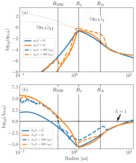
Figure 2: (a) Radial profiles of the diffusion coefficients $\eta_{\mathrm{O}}$ and $\eta_{\mathrm{A}}$ at the mid-plane at $t=0$ (solid) and $t=500~{}t_{\mathrm{K0}}$ (dashed) when the MRI turbulence has been saturated. The diffusion coefficients are shown in the code units. The thin dashed and dotted lines show the diffusion coefficients at $t=0$ derived by chemical reactions with thermal and non-thermal ionization, respectively. Panel (b) is the same as Panel (a) but for the Elsässer numbers $\Lambda_{\mathrm{O}}$ and $\Lambda_{\mathrm{A}}$ at the mid-plane at $t=0$ and $t=500~{}t_{\mathrm{K0}}$. For both panels, the three vertical dashed lines correspond to $R_{\mathrm{MRI}}$, $R_{\eta}$, and $R_{\mathrm{ch}}$ from left to right.

We present the spatial distributions of $\eta_{\mathrm{O}}$ and $\eta_{\mathrm{A}}$ in the initial condition. Figure 2a shows the radial profiles of $\eta_{\mathrm{O}}$ and $\eta_{\mathrm{A}}$ at the mid-plane. Both resistivities show a similar behavior; they increase steeply as a function of the radius, reach maxima around $R\sim 1~{}$au, and then decrease steeply.

Here we define three characteristic radii from the radial profiles of $\eta_{\mathrm{O}}$, $\eta_{\mathrm{A}}$, $\Lambda_{\mathrm{O}}$, and $\Lambda_{\mathrm{A}}$. The first characteristic radius is $R_{\mathrm{MRI}}$ which is the inner edge of the OR dead zone at the mid-plane. As shown in Figure 2b, in the initial condition, the inner dead-zone edges for OR and AD are located in the region where the thermal ionization dominates over the non-thermal ionization. The inner dead-zone edge for OR moves outward until the MRI turbulence is saturated while that for AD do not since $\Lambda_{\mathrm{O}}\propto B^{2}$ and $\Lambda_{\mathrm{A}}\propto B^{0}$, where we use the fact that $\eta_{\mathrm{O}}\propto B^{0}$ and $\eta_{\mathrm{A}}\propto B^{2}$ (Section 2.3.4). In Figure 2b, we plot the radial profiles of $\Lambda_{\mathrm{O}}$ and $\Lambda_{\mathrm{A}}$ at $t=500~{}t_{\mathrm{K0}}$ when the MRI turbulence has been saturated. At $R=R_{\mathrm{MRI}}=0.5~{}\mathrm{au}$, $\Lambda_{\mathrm{O}}$ becomes unity, and $R_{\mathrm{MRI}}$ does not change after the MRI turbulence is saturated. Hereafter, the inner dead-zone edge for OR is simply called the inner dead-zone edge.

The second characteristic radius is $R=R_{\eta}=1.2~{}\mathrm{au}$ around which $\eta_{\mathrm{O}}$ and $\eta_{\mathrm{A}}$ take the largest values and $\Lambda_{\mathrm{O}}$ and $\Lambda_{\mathrm{A}}$ take the lowest values (Figures 2a and 2b). This corresponds to the radius around which the main ionization process switches from the thermal to non-thermal ionization.

The third characteristic radius is $R_{\mathrm{ch}}=3~{}$au beyond which the main negative charge carrier changes from dust grains to electrons (Section 2.3.4).

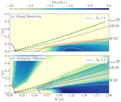
Figure 3: Two-dimensional distributions of (a) $\eta_{\mathrm{O}}$ and (b) $\eta_{\mathrm{A}}$ in the code units at $t=500~{}t_{\mathrm{K0}}$ when the MRI turbulence is saturated. The white dashed lines show the contours of $\eta_{\mathrm{O}}$ and $\eta_{\mathrm{A}}$ at $10^{-4}$ and $10^{-2}$. The conditions of $\Lambda_{\mathrm{O}}=1$ and $\Lambda_{\mathrm{A}}=1$ are displayed by the red and blue lines in Panel (a) and (b), respectively. In each panel, the two black dashed lines correspond to $z=H(R)$ and $z=2H(R)$, and the green dashed line show $z=z_{\mathrm{atm}}(R)$ above which the warm atmospheres exist.

2.3.3 Two Dimensional Distributions of the Diffusion Coefficients

The two-dimensional distributions of $\eta_{\mathrm{O}}$ and $\eta_{\mathrm{A}}$ in the ($R$,$z$) plane at $t=500~{}t_{\mathrm{K0}}$ are displayed in Figures 3a and 3b, respectively. $\eta_{\mathrm{O}}$ decreases from the mid-plane toward upper latitudes because the density decreases. The spatial distribution of $\eta_{\mathrm{A}}$ is different from that of $\eta_{\mathrm{O}}$ especially for $R<1~{}$au, where $\eta_{\mathrm{A}}$ increases from the mid-plane toward upper latitude in the AD dead zone. This comes from the fact that AD is important for strong $B$ and/or low $\rho$ when dust grains do not play an important role in the resistivities.

The shapes of the dead-zone boundaries around the inner edges reflect the physical properties of OR and AD. As the radius increases from the inner boundary of the simulation box, OR makes the disk dead at the mid-plane first around $R\sim R_{\mathrm{MRI}}$ while high latitude regions are the first place which become dead for AD.

The vertical dead-zone boundaries for OR and AD lie between $z=H(R)$ and $z=2H(R)$, and the AD dead-zone is more extended vertically than the OR dead-zone. The base of the warm atmospheres $z=z_{\mathrm{atm}}(R)$ is well above the dead-zone boundaries.

2.3.4 The Dependence of the Diffusion Coefficients on the Field Strength

For OR, $\eta_{\mathrm{O}}$ is independent of $B$ because $B$ in the factor $(ec/B)$ is cancelled with $\beta_{j}\propto B$ in Equation (14). By contrast, $\eta_{\mathrm{A}}$ depends on $B$ in a more complex manner than $\eta_{\mathrm{O}}$ (Xu & Bai, 2016). If there are no dust grains, using the fact that $\beta_{i}\ll\beta_{e}$, one finds that $\eta_{\mathrm{A}}=\beta_{i}\times cB/(4\pi en_{e})\propto B^{2}$ (Salmeron & Wardle, 2003), where $\beta_{i}$ and $\beta_{e}$ are the Hall parameters of ions and electrons, respectively, and $n_{e}$ is the electron number density.

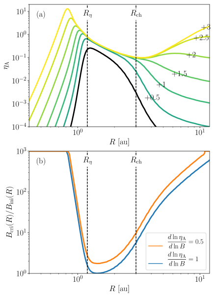
Figure 4: (a) Dependence of $\eta_{\mathrm{A}}$ on the field strength. The radial profiles of $\eta_{\mathrm{A}}$ at the mid-plane are displayed by changing the field strengths. The values of $\log_{10}(B/B_{\mathrm{ini}}(R))$ are labelled on the lines. The vertical axis is shown in the code units. The black line shows the radial profile of $\eta_{\mathrm{A}}$ in the initial condition. (b) The field strengths $B_{\mathrm{cri}}$ where $d\ln\eta_{\mathrm{A}}/d\ln B=1.0$ and $0.5$. For field strengths larger than $B_{\mathrm{cri}}$, the $B$-dependence of $\eta_{\mathrm{A}}$ becomes weak.

The dependence of $\eta_{\mathrm{A}}$ on the field strength is critical in the structure formation of magnetic fields as will be discussed in Section 5.1.2. Development of sharp structures in the magnetic null due to AD has reported in Brandenburg & Zweibel (1994). For such a structure to develop, $\eta_{\mathrm{A}}$ should increase with $B$ so that diffusion near the magnetic null is much more inefficient than in strongly magnetized regions.

Existence of dust grains changes $\eta_{\mathrm{A}}$ significantly. The dependence $\eta_{\mathrm{A}}\propto B^{2}$ is realized at the weak field limit $\beta_{e}\ll 1$ (Xu & Bai, 2016). For $\beta_{e}\gtrsim 1$, $\eta_{\mathrm{A}}$ is not necessarily proportional to $B^{2}$ if the contribution from dust grains to the number density of charged particles is non-negligible. The dependence of $\Lambda_{\mathrm{A}}$ on the field strength for various grain sizes and dust-to-gas mass ratios are shown in Figure 4 of Xu & Bai (2016).

Figure 4a shows how the radial profile of $\eta_{\mathrm{A}}$ at the mid-plane changes as the field strength is increased from the initial value $B_{\mathrm{ini}}(R)$. As $B/B_{\mathrm{ini}}$ increases, $\eta_{\mathrm{A}}$ does not increase in proportional to $B^{2}$, but the increase in $\eta_{\mathrm{A}}$ is saturated especially in the inner region of the dead zone $R_{\eta}\lesssim R\lesssim R_{\mathrm{ch}}$, where the dust grains are the main negative charge carrier. Figure 4b shows the field strengths where $d\ln\eta_{\mathrm{A}}/d\ln B=1$ and $0.5$. For field strengths larger than these critical field strength, the $B$ dependence of $\eta_{\mathrm{A}}$ become weak, leading to inefficient formation of substructures due to AD.

2.4 Methods

To solve the basic equations (1)-(3), we use Athena++ (Stone et al., 2020) which is a complete rewrite of the Athena MHD code (Stone et al., 2008). The HLLD (Harten-Lax-van Leer-Discontinuities) method is used as the MHD Riemann solver (Miyoshi & Kusano, 2005). Magnetic fields are integrated by the constrained transport method (Evans & Hawley, 1988; Gardiner et al., 2008). The second-order Runge-Kutta-Legendre super-time stepping technique is used to calculate the magnetic diffusion processes (Meyers et al., 2014), where the time step is limited so that it is not greater than 30 times the time step determined by OR and AD.

List of the models. Model Name Effective Resolution $t_{\mathrm{end}}$ LowRes $1532\times 1024\times 1024$ $2000t_{\mathrm{K0}}$ HighRes $3064\times 2048\times 2048$ $500t_{\mathrm{K0}}$ The total cell number in each direction if the whole computational domain is resolved with the finest level. The simulations are conducted up to $t_{\mathrm{end}}$.

A spherical-polar coordinate system $(r,\theta,\phi)$ is adopted in the simulation box $r_{\mathrm{in}}\leq r\leq r_{\mathrm{out}}$, $0\leq\theta\leq\pi$, and $0\leq\phi<2\pi$, where $r_{\mathrm{in}}=0.1~{}\mathrm{au}$ and $r_{\mathrm{out}}=12.5~{}\mathrm{au}$. The radial cell width increases with radius by a constant factor so that the radial cell width is almost identical to the zenith one.

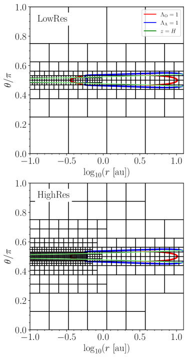
Figure 5: The mesh structures of LowRes and HighRes runs in the $(r,\theta)$ plane. Each cell corresponds to a mesh block with $(N_{r},N_{\theta})=(24,16)$. The red and blue lines represent the boundaries of the dead zones for OR and AD ($\Lambda_{\mathrm{O}}=1$ and $\Lambda_{\mathrm{A}}=1)$, respectively. The green line indicates the scale height $z=\pm H$.

The static mesh refinement technique is used to resolve the disk region which requires high resolution. We adopt two mesh configurations as shown in Figure 5. Each rectangle enclosed by the black lines in Figure 5 consists of $(N_{r},N_{\theta})=(24,16)$. Table ${\dagger}$ ‣ 2.4 lists the models considered in this paper, where $t_{\mathrm{K0}}=2\pi\sqrt{r_{\mathrm{in}}^{3}/GM_{*}}$ is the Kepler rotation period at the inner boundary of the computation box. LowRes run corresponds to the lower resolution simulation where the meshes are refined by 5 levels. If the whole computation domain was divided by the finest cell, the resolution would be $(N_{r},N_{\theta},N_{z})=(1536,1024,1024)$. The disk scale height $H(R)$ is resolved by $19~{}(R/R_{\mathrm{MRI}})^{1/4}~{}\mathrm{cells}$.

LowRes run was conducted until $2000~{}t_{\mathrm{K0}}$ (Table ${\dagger}$ ‣ 2.4). As will be shown in Section A, the resolution of LowRes run is not high enough to obtain the converged MRI turbulence. For comparison, we conduct HighRes run, where the cells in the active zone are further refined in one more higher level (the lower panel of Figure 5). HighRes run could only be calculated to a short time, 500 rotations at the inner boundary, which is long enough for the MRI turbulence to be a saturated state in the active zone.

We note that the resolution of LowRes run is high enough to drive turbulence in the active zone although the saturated $\langle\alpha_{R\phi}\rangle_{H}$ is underestimated by a factor of 2 compared with HighRes run that is expected to give the converged $\langle\alpha_{R\phi}\rangle_{H}$ (Appendix A). In this paper, the long-term evolution is shown on the basis of LowRes run, referring the results of HighRes run to keep the resolution issue in mind.

To prevent the time step $\Delta t$ from being extremely small due to the Alfvén speed, we set the following spatially dependent density floor,

$$\rho(r,\theta,\phi)=\max\left(\rho(r,\theta,\phi),10^{-6}\rho(R,z=0)\right).$$ (25)

This density floor works only in the polar regions. In the other regions, the disk winds keep the densities greater than the floor value.

2.5 Boundary Conditions and Buffer Layer

In Athena++, the boundary conditions are applied by setting the primitive variables in the so-called ghost zones located outside of the computation domain. We impose the following inner boundary conditions. The density and pressure in the ghost cells are fixed to be the initial values, the toroidal velocity follows the rigid rotation $v_{\phi}=\min(R\Omega_{\mathrm{K}}(r_{\mathrm{in}}),v_{\phi,\mathrm{ini}})$, and $v_{r}$ and $v_{\theta}$ are set to zero, where $v_{\phi,\mathrm{ini}}$ is the initial toroidal velocity. We set the boundary conditions for $B_{r}$ and $B_{\phi}$ so that $B_{r}\propto r^{-2}$ and $B_{\phi}\propto r^{-1}$.

The outer boundary conditions are as follows. For the density, pressure, $v_{\theta}$ and $B_{\theta}$, zero-gradient boundary conditions are imposed. We set the boundary conditions for $v_{\phi}$, $B_{r}$, and $B_{\phi}$ so that $v_{\phi}\propto r^{-1/2}$, $B_{r}\propto r^{-2}$, and $B_{\phi}\propto r^{-1}$. The radial velocity is set by using the zero-gradient boundary condition only for $v_{r}>0$ otherwise set to zero.

In order to mitigate the artificial effect of the inner boundary conditions, we introduce a buffer region in $r_{\mathrm{in}}\leq r\leq r_{\mathrm{buf}}$, where $r_{\mathrm{buf}}-r_{\mathrm{in}}=0.025$ au is the width of the buffer region.

The treatment in the buffer region is similar to that of Takasao et al. (2018). The poloidal velocities are damped according to the following equation:

$$\left(\frac{\partial v_{r,\theta}}{\partial t}\right)_{\mathrm{damp}}=-\frac{v_{r,\theta}}{\tau_{\mathrm{d}}(r,\rho)},$$ (26)

where $\tau_{\mathrm{d}}$ is the damping timescale, $\tau_{\mathrm{d}}^{-1}=f_{\mathrm{rad}}(r)f_{v}(v_{r})\tau_{\mathrm{d0}}^{-1}$,

$$f_{\mathrm{rad}}(r)=\frac{1}{2}\left[1-\tanh\left(\frac{r-r_{\mathrm{in}}-d/2}{0.13d}\right)\right],$$ (27)

$$f(v_{r})=\frac{1}{2}\left[\tanh\left(\frac{v_{r}-v_{r,c}}{0.1|v_{r,c}|}\right)+1\right],$$ (28)

and

$$\tau_{\mathrm{d0}}=\max\left[\min\left(f_{\mathrm{d,min}}\frac{\rho}{\rho_{\mathrm{in}}},f_{\mathrm{max}}\right),f_{\mathrm{d,min}}\right]\Omega_{\mathrm{in}}^{-1}.$$ (29)

$f_{\mathrm{d,min}}=1$, $f_{\mathrm{d,max}}=100$, and $v_{r,c}=-0.05v_{\mathrm{K,in}}$. The other physical quantities are unchanged in the damping layer.

2.6 Normalization Units

In this paper, all the physical quantities are normalized by the following three quantities, the length scale $R_{0}=1~{}\mathrm{au}$, the time scale $t_{0}=\sqrt{R_{0}^{3}/GM_{*}}=0.1~{}$yr, and the surface density $\Sigma_{0}=500$ g cm^-2. The gas temperature is normalized by $T_{0}=(\mu m_{\mathrm{H}}/k_{\mathrm{B}})(R_{0}/t_{0})^{2}=6.3\times 10^{5}~{}\mathrm{K}$. Hereafter, we use normalized physical quantities unless otherwise noted except for $R$ and $z$ that are shown in unit of the astronomical unit.

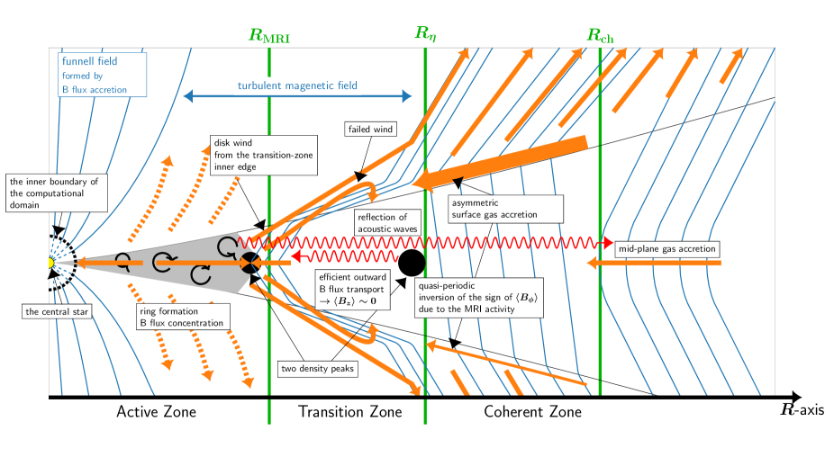
Figure 6: A schematic picture showing our main findings with respect to the time-averaged gas dynamics of the disk. The orange arrows represent the gas motion, and the blue lines show the poloidal magnetic field lines.

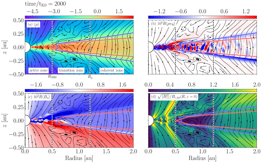
Figure 7: Color maps of (a) $\langle\rho\rangle$, (b) $\langle\rho v_{R}\rangle$, (c) $R\langle B_{R}\rangle$, and (d) $\sqrt{\langle B_{z}\rangle^{2}}/B_{z,\mathrm{ini}}(R,z=0)$ in the inner region in the code units at $t=2000t_{\mathrm{K0}}$, where $B_{z,\mathrm{ini}}(R,z=0)$ is the initial vertical field at the mid-plane. The red (blue) lines correspond to the dead-zone boundaries for OR (AD). The streamlines of the poloidal magnetic fields averaged over $\phi$ are plotted by the black lines. The two vertical dashed lines show $R=R_{\mathrm{MRI}}$ and $R_{\eta}$ from left to right. An animation of this figure is available.

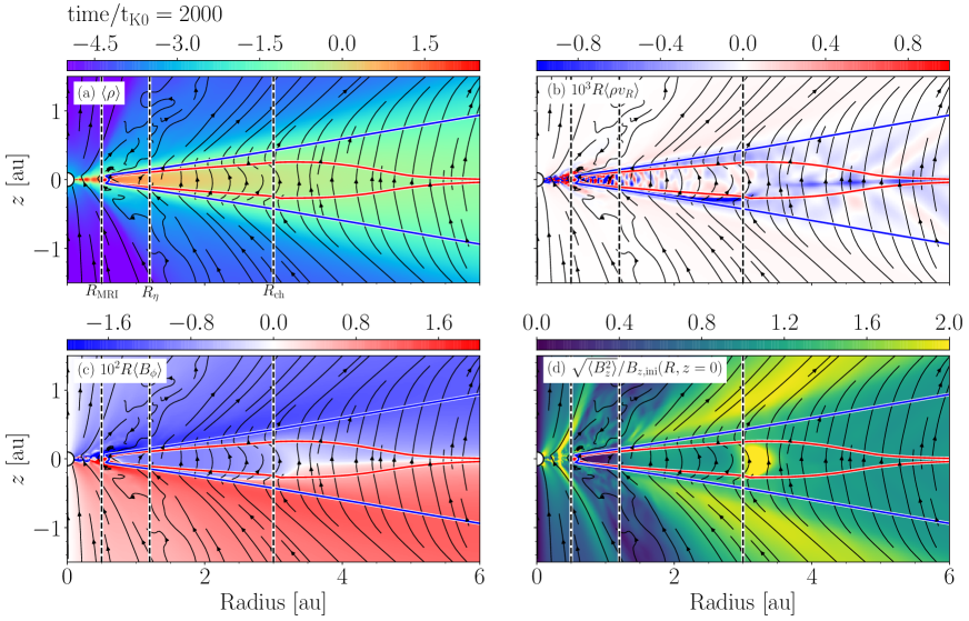
Figure 8: The same as Figure 7 but the radial range $0\leq R\leq 6~{}\mathrm{au}$. The three vertical dashed lines show $R=R_{\mathrm{MRI}}$, $R_{\eta}$, and $R_{\mathrm{ch}}$ from left to right. An animation of this figure is available.

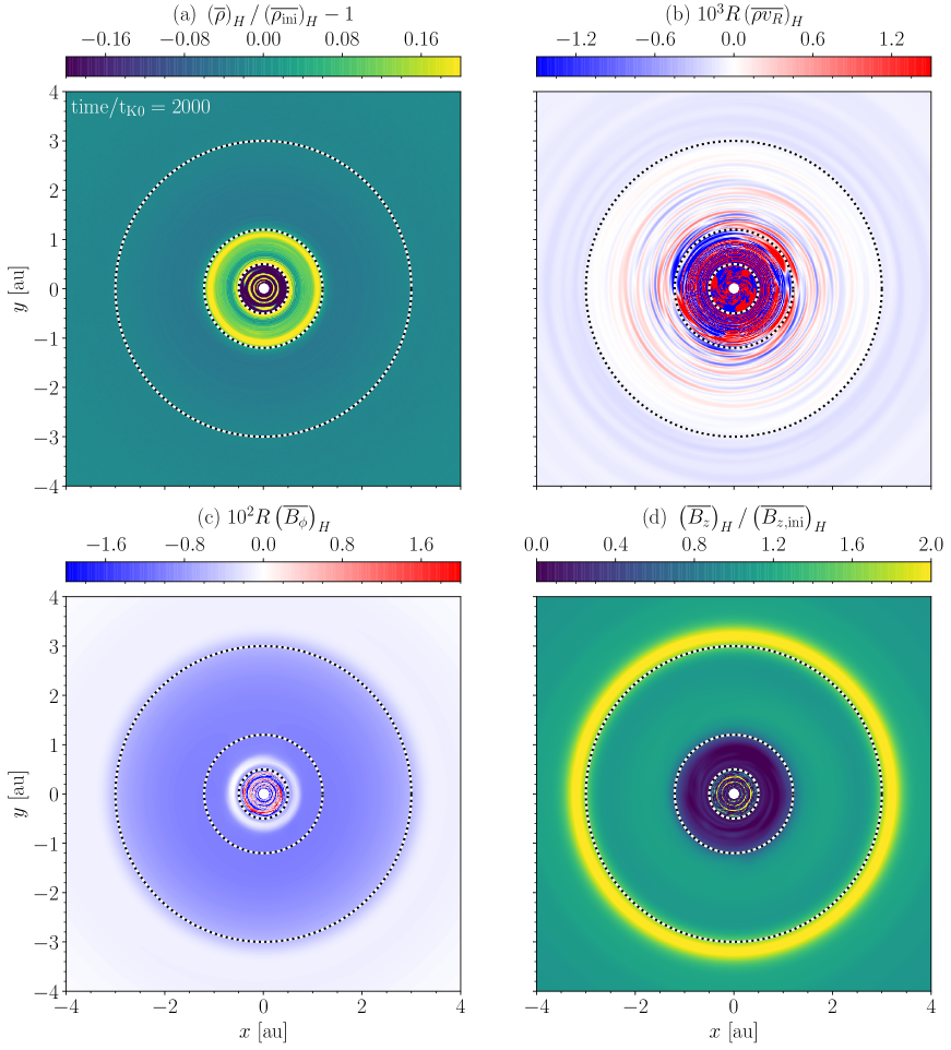
Figure 9: Color maps of (a) the density, (b) the radial mass flux, (c) the toroidal magnetic field, (d) the vertical magnetic field averaged over $|z|\leq H$ at $t=2000~{}t_{\mathrm{K0}}$. All the quantities are shown in the code units. In each panel, the three dashed circles correspond to $R_{\mathrm{MRI}}$, $R_{\eta}$, and $R_{\mathrm{ch}}$ from the center outward. An animation of this figure is available.

2.7 Averaged Quantities

We define averaged quantities used to analyse the simulation results in this section. In the subsequent sections, we present the data converted from the spherical polar coordinates $(r,\theta,\phi)$ to the cylindrical coordinates $(R,\phi,z)$.

We define the data averaged over $\phi$, which are denoted by using angle brackets, or $\langle A\rangle_{\phi}$. Different weight functions are used for different physical quantities in taking averages. For quantities with the dimensions of mass density, momentum density, energy density, and field strength, we take the simple volume-weighted average

$$\langle A\rangle(t,R,z)\equiv\frac{1}{2\pi}\int_{0}^{2\pi}Ad\phi,$$ (30)

where a quantity $A$ can be $\rho$, $\rho v_{z}$, $B_{\phi}^{2}/8\pi$, or $B_{R}$. For velocities and kinetic energies per unit mass, we take the density-weighted average

$$\langle A\rangle(t,R,z)\equiv\left(\int_{0}^{2\pi}\rho d\phi\right)^{-1}\int_{0}^{2\pi}\rho Ad\phi,$$ (31)

where a quantity $A$ can be $v_{z}$ or $v_{R}^{2}/2$.

In order to eliminate stochastic features originating from the MRI turbulence, $\langle A\rangle_{\phi}$ is averaged over $t_{1}\leq t\leq t_{2}$ as follows:

$$\langle A\rangle_{t}(R,z)\equiv\frac{1}{t_{2}-t_{1}}\int_{t_{1}}^{t_{2}}\langle A\rangle dt.$$ (32)

When the radial dependence of the disk structure is investigated, we take the following vertical average of the disk,

$$\langle A\rangle_{z_{\mathrm{b}}}(t,R)\equiv\frac{1}{2z_{\mathrm{b}}}\int_{-z_{\mathrm{b}}}^{z_{\mathrm{b}}}\langle A\rangle dz,$$ (33)

where $z_{\mathrm{b}}$ is a thickness over which $\langle A\rangle$ is averaged.

When the $\phi$ dependence of the physical quantities is investigated, we take the following vertical average over $|z|\leq z_{\mathrm{b}}$,

$$\left(\overline{A}\right)_{z_{\mathrm{b}}}(t,R,\phi)\equiv\frac{1}{2z_{\mathrm{b}}}\int_{-z_{\mathrm{b}}}^{z_{\mathrm{b}}}Adz.$$ (34)

Using $\langle\bm{v}\rangle$ and $\langle\bm{B}\rangle$, we define turbulent components of velocities and magnetic fields as variations from the $\phi$-averaged values as follows;

$$\delta\bm{v}=\bm{v}-\langle\bm{v}\rangle\;\;\mathrm{and}\;\;\delta\bm{B}=\bm{B}-\langle\bm{B}\rangle,$$ (35)

where the turbulent components ($\delta\bm{v}$ and $\delta\bm{B}$) satisfy $\langle\rho\delta\bm{v}\rangle=0$ and $\langle\delta\bm{B}\rangle=0$.

3 Main Results

Figure 6 summarises our findings about the gas dynamics and magnetic field properties in our disks. Details are provided in the subsequent sections.

3.1 Overall Features

In this section, we briefly describe overall features of our results. Figures 7 and 8 show the spatial distributions of the four $\phi$-averaged variables in the inner region of $R\leq 2$ au and outer region of $R\leq 6$ au at $t=2000t_{\mathrm{K0}}$ for LowRes run, respectively. We note that the outer region has not reached a quasi-steady state since 2000 rotations at the inner boundary corresponds to only $12$ rotations at $R=3~{}\mathrm{au}$. Figure 9 shows the face-on color maps of the four vertically-averaged variables.

From Figure 7, in the polar regions of the northern and southern hemispheres, we identify the so-called funnel magnetic fields that are connected with the inner boundary and the magnetic energy dominates over the thermal energy. The radial size of this region increases with time owing to magnetic flux accretion (Beckwith et al., 2009; Takasao et al., 2019). The size of the funnel regions may be overestimated because in reality the funnel magnetic fields come from open fields around the central star, whose size is much smaller than the inner boundary in our simulations.

We found that the conventional dead zone identified by $\Lambda_{\mathrm{O}}\leq 1$ and $\Lambda_{\mathrm{A}}\leq 1$ can be divided into two regions separated by $R=R_{\eta}$. We call the inner region of $R_{\mathrm{MRI}}\leq R\leq R_{\eta}$ ”the transition zone” which has different properties from the conventional dead zone. We call the outer region of $R>R_{\eta}$ ”the coherent zone” which has the same properties as the conventional dead zone.

The overall properties of the active, transition, and coherent zones are briefly summarized in Sections 3.1.1, 3.1.2, and 3.1.3, respectively. In Section 3.1.4, we discuss the influence of the active zone on the outer regions.

3.1.1 Active Zone ($R\leq R_{\mathrm{MRI}}$)

The physical properties of the MRI turbulence in the active zone are consistent with those found in the previous studies. We briefly summarise the physical properties of the MRI turbulence, and detailed descriptions are found in Appendix B.

The vertical structure of the magnetic fields changes around $|z|\sim 2H$. The MRI turbulence generates turbulent magnetic fields for $|z|<2H$ while the magnetic fields become coherent in the upper atmosphere (Suzuki & Inutsuka, 2009). We observe a so-called butterfly structure in the $t$-$z$ diagram of $B_{\phi}$ at a fixed radius (Figure 37). The signs of the toroidal field change quasi-periodically and $B_{\phi}$ drifts toward upper atmospheres.

The MRI turbulence drives gas accretion in the inner region of the active zone. The outer region expands outward by receiving the angular momentum from the inner region (Lynden-Bell & Pringle, 1974). In the upper atmospheres ($|z|>2H$), the magnetic torque of the coherent magnetic field drives coherent gas motion near the surface layers.

One of the striking features of our simulations is the occurrence of multiple ring structures in the density field in the long-term evolution, as shown in Figures 7a and 9a (also see Figure 11). The spatial distributions of the density and $B_{z}$ are anti-correlated; the magnetic fluxes are concentrated in the density gaps. Possible formation mechanisms of these ring structures are investigated in Section 3.2.1 and are discussed in Section 5.1.1.

3.1.2 Transition Zone ($R_{\mathrm{MRI}}<R<R_{\eta}$)

We discover a distinct region, the transition zone, in this simulation. Although it was traditionally classified as a dead zone since $\Lambda_{\mathrm{O}}<1$ and $\Lambda_{\mathrm{A}}<1$ are satisfied in most regions, it has many characteristics not found in conventional dead zones. An interesting feature is found in the magnetic field structures in Figure 7d. The vertical magnetic fields almost completely disappear in $R_{\mathrm{MRI}}\lesssim R\lesssim R_{\eta}$ (Section 3.2.3). Such a region has not been found in the previous studies (Lyra & Mac Low, 2012; Dzyurkevich et al., 2010; Flock et al., 2017) because AD, which was neglected in their work, plays an essential role (Section 3.2.3). The gap in the vertical magnetic fields is almost concentric as shown in Figure 9d.

The disappearance of the vertical magnetic field suppresses surface gas accretion expected in the conventional dead zone (Section 3.2.2). Figure 7b shows disturbances in the radial mass flux although there are no turbulence driving mechanisms. These disturbances originate from the active zone (Pucci et al., 2021), and the net radial mass flux is extremely low when $\langle\rho v_{R}\rangle$ is averaged over time (Section 3.2.2). Thus, in the transition zone, gas accretion does not occur either around the mid-plane or on the surface of the disk.

Figure 9a clearly shows that a density peak appears at each edge of the transition zone, or $R\sim R_{\mathrm{MRI}}$ and $R\sim R_{\eta}$. This structure is formed by a combination of no net radial gas motion in the transition zone and the gas supply from the active zone ($R\leq R_{\mathrm{MRI}}$) and the coherent zone ($R\geq R_{\eta}$). Details will be investigated in Sections 4.1 and 4.2.2.

3.1.3 Coherent Zone ($R\geq R_{\eta}$)

The coherent zone with $R\geq R_{\eta}$ has properties consistent with those of the conventional dead zone found in the literature. The magnetic field lines are smooth and coherent both inside and outside the disk.

Just above the coherent zone, the toroidal magnetic field is amplified by the differential rotation because the magnetic field is relatively coupled with the gas. The magnetic tension force $-B_{z}\partial B_{\phi}/\partial z$ extracts the angular momentum from the gas efficiently, driving surface gas accretion between the OR and AD dead-zone boundaries as shown in Figure 7b (Bai & Stone, 2013; Gressel et al., 2015). The electric current sheet where the sign of $\langle B_{\phi}\rangle$ is reversed is located not at the mid-plane but around the lower AD dead-zone boundary, indicating that the $z$-symmetry adopted in the initial condition is broken (Figure 7c). This is because inside the disk, $\eta_{\mathrm{O}}$ and $\eta_{\mathrm{A}}$ are so large that a current sheet cannot exist inside the coherent zone (Figure 2a). As a result, a current sheet is lifted either upward and downward to the height where $\Lambda_{\mathrm{O}}$ is larger than unity (Bai & Stone, 2013; Bai, 2017). The off-mid-plane current sheet causes the surface gas accretion to be asymmetric with respect to the mid-plane because the magnetic torque exerted in the lower side is stronger than that in the upper side.

The behaviors of the magnetic field change around $R\sim R_{\mathrm{ch}}$. For $R\lesssim R_{\mathrm{ch}}$, the current sheet is located at the lower disk surface as explained before. Beyond $R\sim R_{\mathrm{ch}}$, $\eta_{\mathrm{O}}$ and $\eta_{\mathrm{A}}$ are small enough for the current sheet to remain at the mid-plane. A similar feature was reported in Lesur (2021) who demonstrated that the surface gas accretion (mid-plane gas accretion) occurs for lower (higher) $\Lambda_{\mathrm{O}}$. Figure 8c shows that the toroidal field around the mid-plane at $R>R_{\mathrm{ch}}$ is amplified, resulting in the OR dead-zone shrinking vertically toward the mid-plane. Around the mid-plane, the toroidal magnetic fields are amplified by AD. A similar amplification has been found in Suriano et al. (2018, 2019) and also around the inner edge of the transition zone as discussed in Section 3.2.3. The magnetic tension force $-B_{z}\partial B_{\phi}/\partial z$ drives gas accretion at the mid-plane in $R>R_{\mathrm{ch}}$ (Figure 8b).

3.1.4 Influence of the Active Zone on the Transition and Coherent Zones

The MRI activity in the active zone affects both the velocity and magnetic fields in the outer regions. As mentioned in Section 3.1.2, spatial variations in the radial mass flux inside the disk seen in Figures 7b and 8b are caused by outward propagation of disturbances generated by MRI turbulence (Section 3.2.5).

The MRI activity induces quasi-periodic inversion of the sign of the toroidal magnetic field in the transition zone and the inner part of the coherent zone (Section 3.2.4). This leads to a quasi-periodic switching of the current sheet position between the top and bottom dead-zone boundaries. At $t=2000t_{\mathrm{K0}}$, the toroidal field in the disk is negative (Figures 7c and 8c), but at another time it can be positive. The quasi-periodic disturbance of the field structures does not penetrate beyond $R\sim R_{\mathrm{ch}}$. Comparison between Figures 8c and 8d shows that $\langle B_{z}\rangle$ has a concentration around $R\sim R_{\mathrm{ch}}$. Concentrations in $\langle B_{z}\rangle$ propagate outward following quasi-periodic inversion of the sign of the toroidal magnetic field. Details will be investigated in Section 3.2.4.

3.2 Main Findings

In this section, we present detailed analyses about main findings in our simulations.

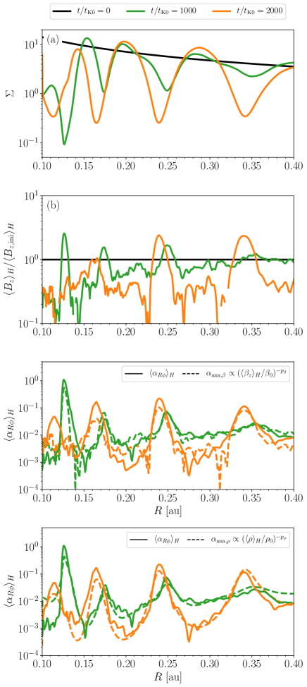
Figure 10: Time evolution of the radial profiles of (a) $\Sigma$, (b) $\langle B_{z}\rangle_{H}/\langle B_{z,\mathrm{ini}}\rangle_{H}$, and (c,d) $\langle\alpha_{R\phi}\rangle$ at $t=1000t_{\mathrm{K0}}$ and $t=2000t_{\mathrm{K0}}$. In Panels (a) and (b), the initial profiles are shown by the black lines. In Panels (c) and (d), the dashed lines show the best-fit functions $\alpha_{\mathrm{ana,\beta}}\propto\langle\beta_{z}\rangle_{H}/\beta_{0})^{-p_{\beta}}$ and $\alpha_{\mathrm{ana,\rho}}=\alpha_{0,\rho}(\langle\rho\rangle_{H}/\rho_{0})^{-p_{\rho}}$, respectively, where $\beta_{0}=10^{4}$ and $\rho_{0}=\rho_{\mathrm{mid,ini}}(R=0.3~{}\mathrm{au})$. The best-fit functions are shown in Table 3.2.1. All the quantities are shown in the code units.

3.2.1 Ring Formation in the Active Zone

We observe the formation of multiple rings and gaps in the active zone as shown in the radial profiles of the column densities $\Sigma$ (Figure 10a). Comparison between Figures 10a and 10b shows that the ring structures in $\Sigma$ are anti-correlated with the radial profile of the vertical magnetic flux averaged over the scale height $\langle B_{z}\rangle_{H}$; the rings (gaps) of $\Sigma$ correspond to the gaps (rings) of $\langle B_{z}\rangle_{H}$.

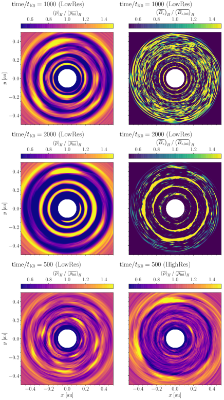
Figure 11: Face-on views of the density (left) and $B_{z}$ (right) averaged over $|z|<H(R)$ at $t/t_{\mathrm{K0}}=1000$ (top) and 2000 (middle). (Bottom) Face-on views of the density averaged over $|z|<H(R)$ at $t=500t_{\mathrm{K0}}$ for LowRes (left) and HighRes (right) runs. All the quantities are shown in the code units.

The top and middle panels of Figure 11 show the face-on views of the density and $B_{z}$ averaged over $|z|<H(R)$. At $t=1000t_{\mathrm{K0}}$, multiple-rings are found in the density map. Thin magnetic flux concentrations are found around $R\sim 0.2~{}$au although the magnetic flux concentrations are not as significant as the variations of the density map. At $t=2000t_{\mathrm{K0}}$, the density contrasts between the rings and gaps become significant, and the magnetic flux concentrations at the density gaps are more prominent than those at $t=1000t_{\mathrm{K0}}$.

The resolution dependence on the density distributions are shown in the bottom panels of Figure 11. Although the density is lower for HighRes run than for LowRes run, ring structures are also found in HighRes run. This suggests that if the long term simulation performed for HighRes run, the ring structures would develop.

Several formation mechanisms of ring structures in the ideal MHD has been proposed. In this section, we examine two mechanisms: the viscous instability (Lightman & Eardley, 1974; Suzuki, 2023) and the wind-driven ring formation (Riols & Lesur, 2019). As shown below, the viscous instability is a possible mechanism of the ring formation found in our simulations while the wind-driven instability may not occur. In Section 5.1.1, we further discuss the origin of the ring structures in our simulations.

Viscous Instability

Viscous instability in MRI-active disks has been investigated in Riols & Lesur (2019) and Suzuki (2023). Riols & Lesur (2019) assumed that the $\alpha$ parameter (Shakura & Sunyaev, 1973) is proportional to $\beta_{z}^{-p_{\beta}}$, where $\beta_{z}=8\pi\langle\langle P\rangle\rangle/\langle\langle B_{z}\rangle\rangle^{2}$ is the plasma beta measured by the net vertical field $\langle\langle B_{z}\rangle\rangle$ since $\alpha$ is anti-correlated with $\beta_{z}$ in local shearing-box simulations (Hawley et al., 1995; Suzuki et al., 2010; Salvesen et al., 2016; Scepi et al., 2018), where $\langle\langle A\rangle\rangle$ is a volume-average of $A$. The instability criterion derived by Riols & Lesur (2019) is $p_{\beta}>1$. Suzuki (2023) extended the linear analysis in Riols & Lesur (2019) by considering the dependence on $\langle\langle\rho\rangle\rangle$ and $\langle\langle B_{z}\rangle\rangle$ separately, or $\alpha\propto\langle\langle\rho\rangle\rangle^{-p_{\rho}}\langle\langle B_{z}\rangle\rangle^{-p_{B_{z}}}$. The instability criterion derived by Suzuki (2023) is $p_{\rho}>1$. $p_{B_{z}}$ does not contributes to the instability criterion, but it changes the growth rate. We note that the instability criteria derived in Riols & Lesur (2019) and Suzuki (2023) are consistent since $\beta_{z}^{-p_{\beta}}\propto\langle\langle\rho\rangle\rangle^{-p_{\beta}}\langle\langle B_{z}\rangle\rangle^{2p_{\beta}}$.

We investigate whether our results satisfy the instability criteria given by Riols & Lesur (2019) and Suzuki (2023). The $\alpha$ parameter is defined by using the thermal pressure, Reynolds stress, and Maxwell stress averaged over $|z|\leq H$ as follows:

$$\langle\alpha_{R\phi}\rangle_{H}=\frac{1}{\langle P\rangle_{H}}\left\{\langle\rho\delta v_{R}\delta v_{\phi}\rangle_{H}+\left\langle-\frac{B_{R}B_{\phi}}{4\pi}\right\rangle_{H}\right\}.$$ (36)

The plasma beta averaged over $z\leq H$ is defined as $\langle\beta_{z}\rangle_{H}=8\pi\langle P\rangle_{H}/\langle B_{z}\rangle_{H}^{2}$. The radial profiles of $\langle\alpha_{R\phi}\rangle_{H}$ are fitted by the two fitting functions $\alpha_{\mathrm{ana,\beta}}\propto(\langle\beta_{z}\rangle_{H}/\beta_{0})^{-p_{\beta}}$ and $\alpha_{\mathrm{ana,\rho}}\propto(\langle\rho\rangle_{H}/\rho_{0})^{-p_{\rho}}$ , where $\beta_{0}=10^{4}$ and $\rho_{0}=\rho_{\mathrm{mid,ini}}(R=0.3~{}\mathrm{au})$. The best-fit functions are shown in Table 3.2.1. Figure 10c (Figure 10d) compares $\langle\alpha_{R\phi}\rangle_{H}$ and the best-fit functions $\alpha_{\mathrm{ana,\beta}}$ ($\alpha_{\mathrm{ana,\rho}}$) at both $t=1000~{}t_{\mathrm{K0}}$ and $2000~{}t_{\mathrm{K0}}$. Figures 10c and 10d show that both fitting functions $\alpha_{\mathrm{ana,\beta}}$ and $\alpha_{\mathrm{ana,\rho}}$ reproduce $\langle\alpha_{R\phi}\rangle_{H}$ reasonably well.

The best-fit functions. $\alpha_{\mathrm{ana,\beta}}$ $\alpha_{\mathrm{ana,\rho}}$ $t=1000t_{\mathrm{K0}}$ $0.013(\langle\beta_{z}\rangle_{H}/\beta_{0})^{-0.41}$ $0.0091(\langle\rho\rangle_{H}/\rho_{0})^{-1.16}$ $t=2000t_{\mathrm{K0}}$ $0.011(\langle\beta_{z}\rangle_{H}/\beta_{0})^{-0.32}$ $0.0022(\langle\rho\rangle_{H}/\rho_{0})^{-1.38}$

Table 3.2.1 shows that the results of LowRes run do not satisfy the Riols & Lesur (2019) instability criterion while they satisfy the Suzuki (2023) instability criterion since $p_{\beta}\sim 0.3-0.4$ and $p_{\rho}>1$. This suggests that the viscous instability may contribute to the ring formations in our simulations if the $\alpha$ parameter is determined by the gas density.

Although a quantitative argument why $p_{\rho}$ becomes greater than unity is still missing, an anti-correlation between $\langle\rho\rangle_{H}$ and $\langle B_{z}\rangle_{H}$ seen in Figures 11a and 11b may be the key to understand the strong density dependence of the $\alpha$ parameter. Similar anti-correlations between the density and the vertical field were reported, for instance, in Bai & Stone (2014), Suriano et al. (2019), Jacquemin-Ide et al. (2021), and Suzuki (2023). Using $\alpha_{\mathrm{ana,\beta}}\propto\langle\beta_{z}\rangle_{H}^{-p_{\beta}}\propto\langle\rho\rangle_{H}^{-p_{\beta}}\langle B_{z}\rangle^{2p_{\beta}}_{H}$ and assuming $\langle B_{z}\rangle_{H}\propto\langle\rho\rangle_{H}^{-q_{B_{z}}}$, we obtain $\alpha_{\mathrm{ana,\beta}}\propto\langle\rho\rangle_{H}^{-p_{\beta}(2q_{B_{z}}+1)}$. When $\langle B_{z}\rangle_{H}$ and $\langle\rho\rangle_{H}$ are anti-correlated ($q_{B_{z}}>0$), the density dependence of $\alpha_{\mathrm{ana,\beta}}$ is apparently stronger than when $\alpha_{\mathrm{ana,\beta}}$ is assumed to be a function of $\langle\beta_{z}\rangle_{H}$. However this simple argument does not quantitatively explain our results. LowRes run shows that $q_{B_{z}}\sim 0.43$ for $t=1000~{}t_{\mathrm{K0}}$ and $\sim 0.95$ for $t=2000~{}t_{\mathrm{K0}}$. One obtains that $-\partial\ln\alpha_{\mathrm{ana,\beta}}/\partial\ln\langle\rho\rangle_{H}=p_{\beta}(2q_{B_{z}}+1)\sim 0.76$ for $t=1000~{}t_{\mathrm{K0}}$ and $\sim 0.93$ for $t=2000~{}t_{\mathrm{K0}}$, and both values are not consistent with $p_{\rho}$ shown in Table 3.2.1.

Wind-driven Instability

Riols & Lesur (2019) proposed a wind-driven instability where disk winds destabilize disks when the amount of gas removed from gap regions due to winds is greater than that supplied by viscous diffusion from ring to gap regions. Local simulations found that both the $\alpha$ parameter and mass loss rate depend negatively on the plasma beta; more strongly magnetized disks yield faster viscous diffusion and more efficient mass loss. Thus, in order for the wind-driven instability to occur, the mass loss rate should has a sensitive dependence on the plasma beta than the viscous diffusion rate.

We here define the normalized mass loss flux due to the disk wind averaged over time as

$$C_{\mathrm{w}}=\frac{\langle\rho v_{n}\rangle_{t}(z=z_{\mathrm{atm}})+(-\langle\rho v_{n}\rangle_{t}(z=-z_{\mathrm{atm}}))}{2\langle\rho_{\mathrm{mid}}c_{\mathrm{s,mid}}\rangle_{t}},$$ (37)

where $v_{n}$ stands for the velocity component perpendicular to the $\pm z_{\mathrm{atm}}$ surfaces (Figures 1 and 3), $\rho_{\mathrm{mid}}$ is the mid-plane density, and $c_{\mathrm{s,mid}}$ is the mid-plane sound speed.

Assuming that both $C_{\mathrm{w}}$ and $\alpha$ are anti-correlated with $\beta_{z}$ and they follow the relations $C_{\mathrm{w}}\propto\beta_{z}^{-p_{\mathrm{w}}}$ and $\alpha\propto\beta_{z}^{-p_{\beta}}$, Riols & Lesur (2019) found that the wind-driven instability occurs when $p_{\mathrm{w}}>p_{\beta}$. Since $p_{\beta}$ is roughly equal to $0.3-0.4$ in our simulations (Figure 10c and Table 3.2.1), $p_{\mathrm{w}}$ needs to be larger than $0.3-0.4$ in order for the wind-driven instability to occur.

Figure 12: (a) Normalized vertical mass loss rate in the active zone $C_{\mathrm{w}}$ defined in Equation (37) as a function of radius. The solid and dashed lines correspond to the radial profiles of $C_{\mathrm{w}}$ where $C_{\mathrm{w}}>0$ and $C_{\mathrm{w}}<0$, respectively. The thin dashed lines show the radial profiles of $\langle\beta_{z,\mathrm{mid}}\rangle_{t}^{-1}$ whose value is shown on the right vertical axis. The data are averaged over $900\leq t/t_{\mathrm{K0}}\leq 1000$ and $1900\leq t/t_{\mathrm{K0}}\leq 2000$. (b) Color maps of $\langle\rho\rangle$ at $t=2000~{}t_{\mathrm{K0}}$. The black lines show the streamlines of the poloidal magnetic field averaged over $\phi$. The two dotted magenta lines correspond to $z=\pm z_{\mathrm{atm}}$.

Figure 12a compares the radial profiles of $C_{\mathrm{w}}$ with the inverse of the time-averaged mid-plane plasma beta $\langle\beta_{z,\mathrm{mid}}\rangle_{t}\equiv 8\pi\langle P\rangle_{t}(z=0)/\langle B_{z}\rangle_{t}^{2}(z=0)$. $C_{\mathrm{w}}$ is poorly correlated with $\langle\beta_{z,\mathrm{mid}}\rangle^{-1}$, indicating that the wind-driven instability is not caused by the disk wind at least in our simulations.

Figure 12a shows that in the gap regions where the radial profiles of $\langle\beta_{z,\mathrm{mid}}\rangle_{t}^{-1}$ have local maxima, $C_{\mathrm{w}}$ is negative, indicating that the gas flows into the density gap regions rather than being ejected from the disk in the vertical direction. Why are there no outflows from the gap regions where the magnetic field is strong? Riols & Lesur (2019) pointed out the gas in the gap regions is ejected by ”wind plumes” where the magnetic fields are strong enough to be coherent and are tilted with respect to the $z$-axis (see also Riols & Lesur, 2018). Figure 12b shows that the poloidal magnetic field structures originating from the gap regions do not maintain a large tilt with respect to the $z$-axis as $|z|$ increase, suggesting that the gas is not continuously accelerated along the field lines.

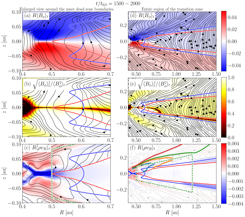
Figure 13: Spatial Structures of $R\langle B_{\phi}\rangle_{t}$ (top), $\sqrt{\langle B_{\phi}\rangle_{t}^{2}/\langle B_{\phi}^{2}\rangle_{t}}$ (middle), and $R\langle\rho v_{R}\rangle_{t}$ (bottom) in the transition zone. The left panels show the enlarged view around the inner dead-zone boundaries, and the right panels display the entire region of the transition zone. The results are averaged over $0\leq\phi<2\pi$ and $1500\leq t/t_{\mathrm{K0}}\leq 2000$, and all the quantities are shown in the code units. In each panel, the red and blue lines represent the OR and AD dead-zone boundaries, respectively. The black lines show the streamlines of the poloidal magnetic fields (the top and middle panels) and poloidal velocity fields (the bottom panels). In the bottom panels, the streamlines of the poloidal velocity fields are not shown inside the OR dead-zone, and the region enclosed by the green dashed lines is used to evaluate the mass transfer in the transition zone (Section 4.2). In Panel (f), the four streamlines originating from $(R,z)=(0.45~{}\mathrm{au},0.06~{}\mathrm{au})$, $(0.45~{}\mathrm{au},0.07~{}\mathrm{au})$, $(0.45~{}\mathrm{au},0.073~{}\mathrm{au})$, and $(0.45~{}\mathrm{au},0.08~{}\mathrm{au})$ are shown by the thick lines.

3.2.2 Disk Wind Launched Around the Transition-zone Inner Edge and Non-existence of Gas Accretion in the Transition Zone

The transition zone is disturbed by the influence from the turbulence in the active zone, and exhibits time variations as will be discussed in Sections 3.2.4 and 3.2.5. In this section, we investigate the quasi-steady structure of the transition zone by taking time average.

The left panels of Figure 13 show the close-up views of the magnetic fields and velocities around the dead-zone inner edge. The MRI turbulence appears to be suppressed around $R\sim 0.45~{}$au, which is slightly different from $R=R_{\mathrm{MRI}}=0.5~{}\mathrm{au}$ defined by $\Lambda_{\mathrm{O}}=1$. This is because MRI turbulence is partially suppressed even where $\Lambda_{\mathrm{O}}$ is slightly greater than unity.

Around the mid-plane in $0.45~{}\mathrm{au}\lesssim R\lesssim 0.55~{}\mathrm{au}$, hourglass-shaped poloidal magnetic fields develop. The vertical distribution of each component of the magnetic field at $R=R_{\mathrm{MRI}}$ is shown in Figure 14a. The toroidal magnetic field dominates over the other components, and has a sharp gradient at the mid-plane.

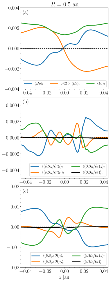
Figure 14: Vertical profiles of (a) $\langle B_{R}\rangle_{t}$, $0.02\langle B_{\phi}\rangle_{t}$, and $\langle B_{z}\rangle_{t}$, (b) $\langle(\partial B_{R}/\partial t)_{\mathrm{I}}\rangle_{t}$, $\langle(\partial B_{R}/\partial t)_{\mathrm{O}}\rangle_{t}$, $\langle(\partial B_{R}/\partial t)_{\mathrm{A}}\rangle_{t}$, $\langle(\partial B_{R}/\partial t)\rangle_{t}$, and (c) $\langle(\partial B_{\phi}/\partial t)_{\mathrm{I}}\rangle_{t}$, $\langle(\partial B_{\phi}/\partial t)_{\mathrm{O}}\rangle_{t}$, $\langle(\partial B_{\phi}/\partial t)_{\mathrm{A}}\rangle_{t}$, $\langle(\partial B_{\phi}/\partial t)\rangle_{t}$ at $R=R_{\mathrm{MRI}}=0.5~{}$au. They are averaged over $1500t_{\mathrm{K0}}\leq t\leq 2000t_{\mathrm{K0}}$. All the quantities are shown in the code units.

AD plays a critical role in the formation of the hourglass-shaped poloidal magnetic fields in $0.45~{}\mathrm{au}\lesssim R\lesssim 0.55~{}\mathrm{au}$. To investigate which of the ideal, OR, and AD terms is the most effective to produce the hourglass-shaped magnetic fields, we measure their contributions to $-\langle\left(\nabla\times\bm{E}\right)_{R}\rangle$, which is equal to $\partial\langle B_{R}\rangle/\partial t$, at a given $z$. First, we focus on the region of $|z|\lesssim 0.01~{}\mathrm{au}$ where the mid-plane gas accretion is seen in Figure 13c. Figure 14b shows that the AD term tilts the poloidal magnetic field toward the radial direction of the disk ($\langle(\partial B_{R}/\partial t)_{\mathrm{A}}\rangle>0$ for $z>0$, and $\langle(\partial B_{R}/\partial t)_{\mathrm{A}}\rangle<0$ for $z<0$), and the ideal MHD term does the same. The vertical profile of $\langle B_{R}\rangle$ is almost stationary by the balance between diffusion due to the OR term and amplification due to the AD and ideal MHD terms. Far from the mid-plane ($|z|\gtrsim 0.02~{}\mathrm{au})$, the AD term behaves quite the opposite. The AD term works as diffusion of $\langle B_{R}\rangle$ amplified by the ideal MHD term.

AD also amplifies the toroidal fields near the mid-plane in $0.45~{}\mathrm{au}\lesssim R\lesssim 0.55~{}\mathrm{au}$. Figure 14c is the same as Figure 14b but for $\langle B_{\phi}\rangle$. Figure 14c shows that the signs of $\langle B_{\phi}\rangle$ and $\langle(\partial B_{\phi}/\partial t)_{\mathrm{A}}\rangle$ are the same near the mid-plane ($|z|\lesssim 0.01~{}\mathrm{au}$), indicating that the AD term amplifies $\langle B_{\phi}\rangle$ and steepens its gradient. The vertical profile of $\langle B_{\phi}\rangle$ is kept almost stationary by the OR term smoothing $\langle B_{\phi}\rangle$. The ideal MHD term partially contributes to the steepening of $\langle B_{\phi}\rangle$. In a similar way as $\langle(\partial B_{R}/\partial t)_{\mathrm{A}}\rangle$, far from the mid-plane, the AD term works as diffusion of $\langle B_{\phi}\rangle$ amplified by the ideal MHD term.

The magnetic torque due to $-B_{z}\partial B_{\phi}/\partial z$ drives mid-plane gas accretion (Figures 13a and 13c). Just above the thin mid-plane gas accretion layer, the wind-like gas flows directing outward are driven. This is also caused by the magnetic torque of the coherent magnetic fields (Blandford & Payne, 1982; Bai et al., 2016). The gas streaming lines at lower latitudes return to the mid-plane. As a result, meridional flows are formed in $0.45~{}\mathrm{au}\lesssim R\lesssim 0.5~{}\mathrm{au}$ and $|z|\lesssim 0.05~{}\mathrm{au}$; the streamlines of the gas flows are circulated each in the north and south sides of the disk as shown in Figure 13c.

The right panels of Figure 13 zooms out the region shown in the left panels to cover the entire transition zone. Four streamlines are highlighted by colors with thick lines in Figure 13f. One can find that the lower two streamlines correspond to failed disk winds; the material does not reach the outer boundary of the simulation domain but falls back on to the disk surface in $R\lesssim R_{\eta}$ by the central star gravity (Takasao et al., 2018). By contrast, the disk wind flowing from the higher latitudes ($z=0.073~{}\mathrm{au}$ and $0.08~{}\mathrm{au}$, green and red) reaches the outer boundary of the simulations box. The directions of the winds are not parallel to the poloidal magnetic fields owing to AD (Figure 14b).

Comparison between Figures 13f and 7b shows that the radial mass flux inside the OR dead-zone disappears when the time average is taken. The radial mass flux existing inside the OR dead-zone in Figure 7b originates from the sound waves generated from the MRI turbulence in the active zone (Section 3.2.5 and Pucci et al., 2021).

3.2.3 Disappearance of the Vertical Magnetic Flux in the Transition Zone

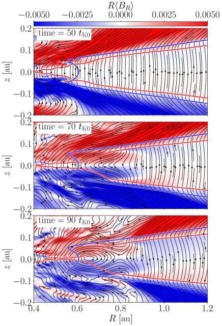
Figure 15: Time sequence of the $\phi$-averaged field structure near the dead zone boundary from $t/t_{\mathrm{K0}}=50$ to $90$. In each panel, the colors show the $R\langle B_{R}\rangle$ map, and the black lines correspond to the streamline of the poloidal magnetic fields. The values of $R\langle B_{R}\rangle$ are shown in the code units.

In this section, we investigate how the vertical flux disappears in the transition zone (Figures 7d and 9d). This flux transport is very efficient, and occurs in less time than 7 rotations at $R=R_{\mathrm{MRI}}$.

Figure 15 shows the time sequence of the magnetic field structure. At $t=50t_{\mathrm{K0}}$, the poloidal magnetic field lines are almost vertical inside the AD dead zone at $R>0.6~{}\mathrm{au}$. After 1.8 rotations at $R=R_{\mathrm{MRI}}$ ($t=70t_{\mathrm{K0}}$), the poloidal magnetic fields are highly inclined and their directions are almost horizontal in $0.6~{}\mathrm{au}\lesssim R\lesssim 0.8~{}\mathrm{au}$. Inside the transition zone, the radial magnetic fields are amplified. At $t=90~{}t_{\mathrm{K0}}$, the magnetic loop structure whose center is at $R=0.62~{}\mathrm{au}$ and $z=0$ is formed. The time evolution shown in Figure 15 occurs on a dynamical timescale at $R=0.6~{}$au.

In order to investigate the evolution of the magnetic fields, the vertical profiles of the $\phi$-averaged magnetic fields at $R=0.7$ au are shown in Figure 16. As shown in Figure 15, $\langle B_{R}\rangle$ is amplified around the mid-plane during $50\leq t/t_{\mathrm{K0}}\leq 70$. At the same time, $\langle B_{\phi}\rangle$ is also amplified. Interestingly, $\langle B_{z}\rangle$ decreases while $\langle B_{R}\rangle$ and $\langle B_{\phi}\rangle$ are amplified, indicating a rapid transport of the vertical field.

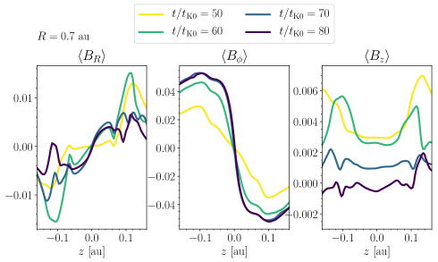
Figure 16: Time evolution of the vertical profiles of $\langle B_{R}\rangle$, $\langle B_{\phi}\rangle$, and $\langle B_{z}\rangle$ at $R=0.7$ au from $t/t_{\mathrm{K0}}=50$ to $80$ in an interval of 10. All the quantities are shown in the code units.

What causes this magnetic field evolution? The answer can be obtained from the $\phi$-averaged induction equations, which are given by

$$\frac{\partial\langle B_{R}\rangle}{\partial t}=\frac{\partial\langle E_{\phi}\rangle}{\partial z},$$ (38)

$$\frac{\partial\langle B_{\phi}\rangle}{\partial t}=-\frac{\partial\langle E_{R}\rangle}{\partial z}+\frac{\partial\langle E_{z}\rangle}{\partial R},$$ (39)

and

$$\frac{\partial\langle B_{z}\rangle}{\partial t}=-\frac{1}{R}\frac{\partial(R\langle E_{\phi}\rangle)}{\partial R}.$$ (40)

The electric field can be divided into three components,

$$\bm{E}=\bm{E}_{\mathrm{I}}+\bm{E}_{\mathrm{O}}+\bm{E}_{\mathrm{A}},$$ (41)

where $\bm{E}_{\mathrm{I}}=-\bm{v}\times\bm{B}$ is the electric field in the ideal MHD, $\bm{E}_{\mathrm{O}}=\eta_{\mathrm{O}}\bm{J}$ and $\bm{E}_{\mathrm{A}}=\eta_{\mathrm{O}}\bm{J}_{\perp}$ are the electric fields caused by OR and AD, respectively.

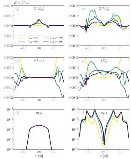
Figure 17: Time evolution of the vertical profiles of (a) $\langle\left(E_{\phi}\right)_{\mathrm{O}}\rangle$, (b) $\langle\left(E_{\phi}\right)_{\mathrm{A}}\rangle$, (c) $\langle\left(E_{\phi}\right)_{\mathrm{I}}\rangle$, (d) $\langle E_{\phi}\rangle$, (e) $\langle\eta_{\mathrm{O}}\rangle$, and (f) $\langle\eta_{\mathrm{A}}\rangle$ at $R=0.7$ au from $t/t_{\mathrm{K0}}=50$ to $80$ in an interval of 10. All the quantities are shown in the code units.

The evolution of the vertical field is determined by Equation (40). In the early evolution, $\langle(E_{\phi})_{\mathrm{O}}\rangle$ provides a dominant contribution to $\langle E_{\phi}\rangle$ as will be shown in Figure 18. Because $|\partial B_{R}/\partial z|$ dominates over $|\partial B_{z}/\partial R|$

$$\langle(E_{\phi})_{\mathrm{O}}\rangle\sim\bigl{\langle}{\eta_{\mathrm{O}}\frac{\partial B_{R}}{\partial z}}\bigr{\rangle},$$ (42)

the vertical distribution of $B_{R}$ is critical for the vertical field transport.

The evolution of $\langle B_{R}\rangle$ is determined by the vertical structure of $\langle E_{\phi}\rangle$ (Equation (38)). Around the mid-plane, $\langle\left(E_{\phi}\right)_{\mathrm{I}}\rangle$ is negligible since this region is inside the dead zones. For $t\leq 60~{}t_{\mathrm{K0}}$, $\langle\left(E_{\phi}\right)_{\mathrm{A}}\rangle$ mainly contributes to $\langle E_{\phi}\rangle$. Around the mid-plane, $\partial\langle\left(E_{\phi}\right)_{\mathrm{A}}\rangle/\partial z$ is positive (negative) for $z>0$ ($<0$), leading to amplification of $\langle B_{R}\rangle$ since the signs of $\partial\langle\left(E_{\phi}\right)_{\mathrm{A}}\rangle/\partial z$ and $\langle B_{R}\rangle$ are the same (the left panel of Figure 16). This downward-facing convex profile of $\langle\left(E_{\phi}\right)_{\mathrm{A}}\rangle$ is attributed to the profile of $\langle\eta_{\mathrm{A}}\rangle$, which increases toward upper low density regions (Figure 16f). Since $\langle\eta_{\mathrm{A}}\rangle$ is proportional to $B^{2}$ in this region, the gradient of $\langle\eta_{\mathrm{A}}\rangle$ becomes steeper and steeper owing to the amplification of the magnetic field. As both $\langle B_{R}\rangle$ and $\langle B_{\phi}\rangle$ increase (Figure 16), the current density is enhanced around the mid-plane, and the electric field owing to OR becomes important. For $t\geq 70t_{\mathrm{K0}}$, the downward-facing convex profiles disappear in the $\langle E_{\phi}\rangle$ profile since the downward-facing convex part in $\langle\left(E_{\phi}\right)_{\mathrm{A}}\rangle$ is almost compensated by the upward-facing convex part in $\langle\left(E_{\phi}\right)_{\mathrm{O}}\rangle$. As a result, OR suppresses the amplification of $\langle B_{R}\rangle$.

The gradient of $\langle B_{R}\rangle$ with respect to $z$ become steeper as the time passes, leading that the current sheet around the mid-plane becomes thinner around the central region where the magnetic fields are weak. Development of such sharp structures in the magnetic null by AD was previously reported in Brandenburg & Zweibel (1994).

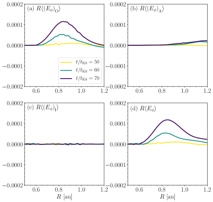
Figure 18: Time Evolution of the radial profiles of the toroidal electric fields, (a) $R\langle\left(E_{\phi}\right)_{\mathrm{O}}\rangle$, (b) $R\langle\left(E_{\phi}\right)_{\mathrm{A}}\rangle$, (c) $R\langle\left(E_{\phi}\right)_{\mathrm{I}}\rangle$, and (d) $R\langle\left(E_{\phi}\right)\rangle$ at the mid-plane at $t/t_{\mathrm{K0}}=50$, 60, and 70. All the quantities are shown in the code units.

Finally, we investigate the radial transport of the vertical field. Equation (40) shows that the transport velocity of $\langle B_{z}\rangle$ is estimated by $\langle E_{\phi}\rangle/\langle B_{z}\rangle$. Since $\langle B_{z}\rangle$ is positive in most regions at the mid-plane, the sign of $\langle E_{\phi}\rangle$ indicates the direction of the vertical field transport. Figure 18 shows the time evolution of the radial profiles of the toroidal electric fields at the mid-plane. OR mainly contributes to $\langle E_{\phi}\rangle$ while $\langle E_{\phi}\rangle_{\mathrm{I}}$ is negligible at the mid-plane where OR suppresses the MRI. AD plays a minor role in $\langle E_{\phi}\rangle$ except for $R\gtrsim 1~{}\mathrm{au}$. A sharp increase in $\langle E_{\phi}\rangle$ in $R\lesssim 0.9~{}\mathrm{au}$ is attributed to a strong radial dependence of $\langle\eta_{\mathrm{O}}\rangle$ in $R<R_{\eta}$ (Figure 2). The radial gradient of $R\langle E_{\phi}\rangle$ around $R\sim 0.8~{}\mathrm{au}$ increases with time from $t\sim 50~{}t_{\mathrm{K0}}$ to $70~{}t_{\mathrm{K0}}$, representing the rapid outward transport of $\langle B_{z}\rangle$ (Figure 16). The rapid outward transport of the vertical field in the transition zone is due to steepening of the vertical gradient of $B_{R}$ around the mid-plane by AD as seen in Figures 16 and 17.

3.2.4 Quasi-periodic Disturbances of Magnetic Fields Beyond the Inner Dead-zone Edge due to the MRI Activity

The turbulence and dynamo activity in the active zone drives time variation in the transition and coherent zones. Figure 19 shows the radius-time diagrams of $\langle B_{z}\rangle_{H}$ and $\langle B_{\phi}\rangle_{H}$. As shown in Section 3.2.1, in the active zone ($R\leq R_{\mathrm{MRI}}$), the ring and gap structures develop in $\langle B_{z}\rangle_{H}$ and $\langle\rho\rangle_{H}$.

In the transition zone ($R_{\mathrm{MRI}}<R<R_{\eta}$), as shown in Section 3.2.3, the combination of OR and AD causes the magnetic flux to be transferred outward rapidly in the early evolution $\sim 100t_{\mathrm{K0}}$. As a result, $\langle B_{z}\rangle_{H}$ is almost zero in the transition zone. The gap structure is maintained at least during the simulation.

Before showing the evolution of $\langle B_{\phi}\rangle_{H}$, we recall the spatial structure of the magnetic fields found in Figures 7c and 13d. Just outside the inner edge of the transition zone, $B_{\phi}$ is amplified above and below the mid-plane, and the current sheet where the sign of $B_{\phi}$ is flipped is located around the mid-plane. As shown in Figure 14, the profile of $B_{\phi}$ is determined by the balance between dissipation of $B_{\phi}$ due to OR and $B_{\phi}$ amplification due to AD and the induction term. For $R\gtrsim 0.7~{}\mathrm{au}$, strong magnetic diffusion moves the current sheet to either upper or lower AD dead-zone boundaries (Figure 7c).

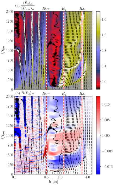
Figure 19: Radius-time diagrams of (a)$\langle B_{z}\rangle_{H}/\langle B_{z,\mathrm{ini}}\rangle_{H}$ and (b)$R\langle B_{\phi}\rangle_{H}$, where $\langle B_{z,\mathrm{ini}}\rangle_{H}$ is $\langle B_{z}\rangle_{H}$ at $t=0$. The vertical red dashed lines correspond to $R_{\mathrm{MRI}}$, $R_{\eta}$, and $R_{\mathrm{ch}}$ from left to right. The black dashed lines show the contours of $\Psi_{\mathrm{rad}}$, which is defined in Equation (61). They correspond to the trajectory of the magnetic flux originated at each equally-spaced position at $t=0$. All the quantities are shown in the code units.

Figure 19b shows that $\langle B_{\phi}\rangle_{H}$ just outside the inner edge of the transition zone changes their sign quasi-periodically. Since the position where $\langle B_{\phi}\rangle=0$ is around the mid-plane, the quasi-periodic variations of $\langle B_{\phi}\rangle_{H}$ are not caused by change of the current sheet position. The vertical profile of $\langle B_{\phi}\rangle$ is not perfectly inversely symmetric with respect to the mid-plane, and the difference between $|\langle B_{\phi}\rangle|$ for $z>0$ and for $z<0$ varies quasi-periodically.

Figure 19b shows that the variations of $\langle B_{\phi}\rangle_{H}$ propagate outward rapidly in the radial direction while they do not propagate beyond $R\sim R_{\mathrm{ch}}$. These $\langle B_{\phi}\rangle_{H}$ variations occur quasi-periodically. The flip of the sign of $\langle B_{\phi}\rangle_{H}$ occurs almost synchronously in $R_{\mathrm{MRI}}\lesssim R\lesssim R_{\mathrm{ch}}$ around $t\sim 150~{}t_{\mathrm{K0}}=13.4~{}t_{\mathrm{K}}(R_{\mathrm{MRI}})$, $\sim 520~{}t_{\mathrm{K0}}=46.5~{}t_{\mathrm{K}}(R_{\mathrm{MRI}})$, $\sim 1100~{}t_{\mathrm{K0}}=98.4~{}t_{\mathrm{K}}(R_{\mathrm{MRI}})$, and $\sim 1450~{}t_{\mathrm{K0}}=130~{}t_{\mathrm{K}}(R_{\mathrm{MRI}})$.

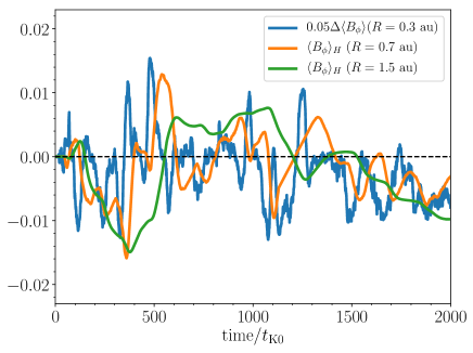
Figure 20: Time variations of $B_{\phi}$ at three different radii. The blue line shows $\Delta\langle B_{\phi}\rangle\equiv\langle B_{\phi}\rangle(z=-2.5H)+\langle B_{\phi}\rangle(z=2.5H)$ at $R=0.3~{}\mathrm{au}$, and $\Delta\langle B_{\phi}\rangle$ is multiplied by 0.05 to facilitate comparison with the other two lines. The orange and green lines correspond to $\langle B_{\phi}\rangle_{H}$ at $R=0.7$ au and $1.5$ au, respectively. All the quantities are shown in the code units.

In order to investigate the origin of the quasi-periodic time variation in $\langle B_{\phi}\rangle_{H}$ in $R_{\mathrm{MRI}}\lesssim R\lesssim R_{\mathrm{ch}}$, we compare the time variations of $B_{\phi}$ at three different radii, $R=0.3$ au, 0.7 au, and 1.5 au. In the active zone, net toroidal field $\langle B_{\phi}\rangle$ is almost zero for $|z|\leq 2H$ because of the MRI turbulence, and the quasi-periodic variations of $\langle B_{\phi}\rangle$ are seen in higher latitudes as the butterfly structure in the time-$z$ diagram (see Figure 37a). In order to quantify the time variations of $\langle B_{\phi}\rangle$, we define $\Delta\langle B_{\phi}\rangle\equiv\langle B_{\phi}\rangle(z=-2.5H)+\langle B_{\phi}\rangle(z=2.5H)$ at $R=0.3~{}\mathrm{au}$. Since the signs of $\langle B\rangle_{\phi}$ in $z>0$ and $z<0$ are opposite, $\Delta\langle B_{\phi}\rangle$ is a measure of the antisymmetry of $\langle B_{\phi}\rangle$ with respect to the mid-plane.

Figure 20 shows that the time variations of $\Delta\langle B_{\phi}\rangle$ at $R=0.3~{}\mathrm{au}$ are correlated with those of $\langle B_{\phi}\rangle_{H}$ at $R=0.7~{}\mathrm{au}$. This means that the drift of the magnetic fields in the active zone disturbs the transition zone. The variations of $\langle B_{\phi}\rangle_{H}$ in the transition zone propagate rapidly in the radial direction owing to efficient magnetic diffusion. This behavior can be seen in Figure 20 that shows a correlation between $\langle B_{\phi}\rangle_{H}$ at $R=1.5$ au and $\langle B_{\phi}\rangle_{H}$ at $R=0.7~{}$au.

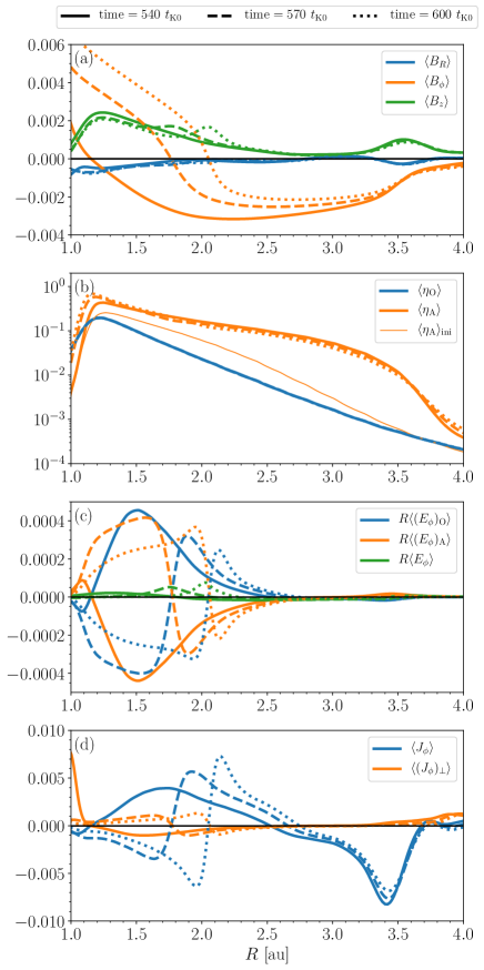
Figure 21: Radial profiles of quantities related to diffusion of the magnetic fields in the coherent zone. In each panel, the solid, dashed, and dotted lines correspond to the results at the mid-plane at $t=540~{}t_{\mathrm{K0}}$, $570~{}t_{\mathrm{K0}}$, and $600~{}t_{\mathrm{K0}}$, respectively. (a) Radial profiles of $\langle B_{R}\rangle$, $\langle B_{\phi}\rangle$, and $\langle B_{z}\rangle$. (b) Radial profiles of $\langle\eta_{\mathrm{O}}\rangle$ and $\langle\eta_{\mathrm{A}}\rangle$. The thin solid orange line shows the radial profile of $\langle\eta_{\mathrm{A}}\rangle$ at the initial condition. (c) Radial profiles of $R\langle(E_{\phi})_{\mathrm{O}}\rangle$, $R\langle(E_{\phi})_{\mathrm{A}}\rangle$, and $R\langle E_{\phi}\rangle=R\left[\langle(E_{\phi})_{\mathrm{I}}\rangle+\langle(E_{\phi})_{\mathrm{O}}\rangle+\langle(E_{\phi})_{\mathrm{A}}\rangle\right]$. They determine the radial diffusion of $\langle B_{z}\rangle$. (d) Radial profiles of $\langle J_{\phi}\rangle$ and $\langle(J_{\phi})_{\perp}\rangle$. All the quantities are shown in the code units.

Next, we investigate the radial diffusion of the magnetic fields in the coherent zone ($R>R_{\eta}$). We focus on the second flip of $\langle B_{\phi}\rangle_{H}$ starting around $t\sim 500~{}t_{\mathrm{K0}}$ (Figure 19b).

Figure 21a shows the time evolution of the radial profiles of $\langle B_{R}\rangle$, $\langle B_{\phi}\rangle$, and $\langle B_{z}\rangle$ at the mid-plane. When the time passes from $t=540~{}t_{\mathrm{K0}}$ to $600~{}t_{\mathrm{K0}}$, the radius where the sign of $\langle B_{\phi}\rangle$ is reversed moves outward while $\langle B_{R}\rangle$ and $\langle B_{z}\rangle$ do not change significantly. At $t=600~{}t_{\mathrm{K0}}$, a concentration of $\langle B_{z}\rangle$ appears around $R\sim 2.1~{}\mathrm{au}$ where the sign of $\langle B_{\phi}\rangle$ is flipped.

The radial diffusion speed of $\langle B_{\phi}\rangle$ is roughly estimated by $\langle\eta_{\mathrm{O}}\rangle$ and $\langle\eta_{\mathrm{A}}\rangle$, which are shown in Figure 21b. $\langle\eta_{\mathrm{A}}\rangle$ increases by increasing the field strength while $\langle\eta_{\mathrm{O}}\rangle$ does not change in time significantly. Around $R\sim 1.2~{}\mathrm{au}$, $\langle\eta_{\mathrm{O}}\rangle$ and $\langle\eta_{\mathrm{A}}\rangle$ are both roughly $\sim 0.3$. The spatial scale of the spatial variation of $\langle B_{\phi}\rangle$ is around $\Delta R\sim 0.5~{}\mathrm{au}$. The typical speed of the radial diffusion of the magnetic fields is estimated to be $\langle\eta\rangle/\Delta R\sim 0.1~{}\mathrm{au}~{}t_{\mathrm{K0}}^{-1}$, indicating that the structure of $\langle B_{\phi}\rangle$ moves 1 au per $10~{}t_{\mathrm{K0}}$. Although this speed is a few times larger than estimated from Figure 21a, they are consistent based on the rough estimate.

The $\langle B_{z}\rangle$ concentration is determined by $R\langle E_{\phi}\rangle$. Figure 21c shows the radial profiles of $R\langle E_{\phi}\rangle$ and the contributions of OR and AD to $R\langle E_{\phi}\rangle$ which are denoted by $R\langle(E_{\phi})_{\mathrm{O}}\rangle$ and $R\langle(E_{\phi})_{\mathrm{A}}\rangle$, respectively. The contribution from the ideal-MHD (induction) term $-\bm{v}\times\bm{B}$ is not plotted in Figure 21c because it is negligible. Figure 21c shows that $R\langle(E_{\phi})_{\mathrm{O}}\rangle$ and $R\langle(E_{\phi})_{\mathrm{A}}\rangle$ have opposite signs and nearly cancel each other. This indicates that AD behaves anti-diffusion since OR provides pure diffusion of magnetic fields. As shown in Figure 21d, the opposite sign of $R\langle(E_{\phi})_{\mathrm{O}}\rangle$ and $R\langle(E_{\phi})_{\mathrm{A}}\rangle$ comes from the fact that the sign of $\langle J_{\phi}\rangle$ is opposite to $\langle(J_{\phi})_{\perp}\rangle$ since $\langle(E_{\phi})_{\mathrm{O}}\rangle\propto\langle J_{\phi}\rangle$. and $\langle(E_{\phi})_{\mathrm{A}}\rangle\propto\langle J_{\phi}\rangle_{\perp}$. This feature was previously pointed out by Béthune et al. (2017). Anti-diffusion owing to AD is not completely cancelled out by the normal diffusion owing to OR, and triggers the concentration of $\langle B_{z}\rangle$.

Comparison between Figures 19a and 19b shows that the concentrations of $\langle B_{z}\rangle_{H}$ are located at the radii where the sign of $\langle B_{\phi}\rangle_{H}$ is flipped for $R\gtrsim R_{\eta}$. The outward propagation of the concentrations of $\langle B_{z}\rangle_{H}$ slows down as the radius increases, and almost stall around $R\sim R_{\mathrm{ch}}$. This is because $\eta_{\mathrm{A}}$ decreases rapidly beyond $R=R_{\mathrm{ch}}$, resulting in a rapid decrease of the propagation speed of the condensations of $\langle B_{z}\rangle_{H}$.

3.2.5 Radial Propagation of the Velocity Disturbances Originating from the MRI Turbulence

The MRI turbulence driven in the active zone generates velocity disturbances that propagate outward and disturb the transition and coherent zones as seen in Figure 7b and 8b.

Figure 22a shows the Mach numbers of the velocity dispersion in the $R$, $\phi$, and $z$ directions at the mid-plane. They are defined as

$$\langle\delta{\cal M}_{R,\phi,z}\rangle=\sqrt{\frac{\bigl{\langle}{\rho\delta v_{R,\phi,z}^{2}}\bigr{\rangle}}{\langle P\rangle}}.$$ (43)

Inside the active zone, $\langle{\cal M}_{R,\phi,z}\rangle$ are as large as $\sim 0.1$. Comparison between the Mach numbers and density in Figure 22a shows that the velocity dispersion is anti-correlated with the density; it is larger in the gaps than in the rings.

Inside the transition zone ($R_{\mathrm{MRI}}<R<R_{\eta}$), $\langle\delta{\cal M}_{R}\rangle$, $\langle\delta{\cal M}_{\phi}\rangle$, and $\langle\delta{\cal M}_{z}\rangle$ behave differently. $\langle\delta{\cal M}_{R}\rangle$ continues to decrease in the transition zone, and reaches $\sim 10^{-2}$ at $R=R_{\eta}$. By contrast, after the rapid decrease at $R\approx R_{\mathrm{MRI}}$, $\langle\delta{\cal M}_{\phi}\rangle$ and $\langle\delta{\cal M}_{z}\rangle$ become almost constant in the outer part of the transition zone. Around $R=R_{\eta}$, all the components of the Mach numbers have a similar value of $\sim 10^{-2}$.

In the coherent zone ($R\geq R_{\eta}$), $\langle\delta{\cal M}_{R}\rangle$ and $\langle\delta{\cal M}_{z}\rangle$ are of similar magnitude and decrease with increasing radius. $\langle\delta{\cal M}_{\phi}\rangle$ is smaller than the other two.

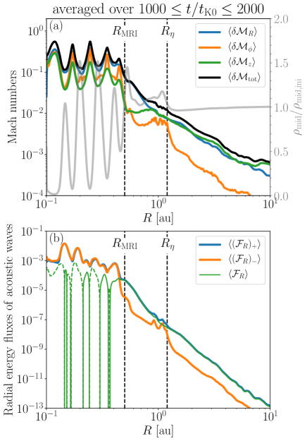
Figure 22: Radial propagation of the sound waves in the whole disk. (a) The Mach numbers in the $R$, $\phi$, and $z$ directions at the mid-plane as a function of $R$ (the left vertical axis). The radial profile of the mid-plane density is shown by the gray line (the right vertical axis). (b) The radial profiles of the energy fluxes of the sound waves. The blue, orange, and green lines correspond to $\langle({\cal F}_{R})_{+}\rangle$, $\langle({\cal F}_{R})_{-}\rangle$, and $\langle{\cal F}_{R}\rangle$ at the mid-plane, respectively. In all the panels, all the data are averaged over $1000\leq t/t_{\mathrm{K0}}\leq 2000$, and the vertical dashed lines denote $R=R_{\mathrm{MRI}}$ and $R_{\eta}$ from left to right. All the quantities are shown in the code units.

We investigate the radial propagation of the radial velocity fluctuations. The energy flux of the sound waves is estimated as

$$\langle{\cal F}_{R}\rangle=\langle\delta\rho\delta v_{R}\rangle c_{\mathrm{s}}^{2},$$ (44)

where $\delta\rho\equiv\rho-\langle\rho\rangle$. It can be divided into the energy flux propagating in the $+R$ direction

$$\langle\left({\cal F}_{R}\right)_{+}\rangle=c_{\mathrm{s}}\biggl{\langle}\rho\left\{\frac{1}{2}\left(\delta v_{R}+c_{\mathrm{s}}\frac{{\delta\rho}}{\langle\rho\rangle}\right)\right\}^{2}\biggr{\rangle},$$ (45)

and that propagating in the $-R$ direction

$$\langle\left({\cal F}_{R}\right)_{-}\rangle=c_{\mathrm{s}}\biggl{\langle}\rho\left\{\frac{1}{2}\left(\delta v_{R}-c_{\mathrm{s}}\frac{{\delta\rho}}{\langle\rho\rangle}\right)\right\}^{2}\biggr{\rangle}.$$ (46)

They satisfy $\langle{\cal F}_{R}\rangle=\langle({\cal F}_{R})_{+}\rangle-\langle({\cal F}_{R})_{-}\rangle$.

The radial distributions of $\langle({\cal F}_{R})_{+}\rangle$, $\langle({\cal F}_{R})_{-}\rangle$, and $\langle{\cal F}_{R}\rangle$ are shown in Figure 22b. In the active zone, $\langle({\cal F}_{R})_{+}\rangle$ and $\langle({\cal F}_{R})_{-}\rangle$ are comparable; there are equal amounts of outward and inward propagating sound waves.

Outside the active zone, $\langle({\cal F}_{R})_{+}\rangle$ dominates over $\langle({\cal F}_{R})_{-}\rangle$. This clearly shows that the sound waves transport more energy outward. Around $R\sim R_{\eta}$, $\langle({\cal F}_{R})_{-}\rangle$ is enhanced and becomes comparable to $\langle({\cal F}_{R})_{+}\rangle$ although the outward flux is still larger than the inward flux. This indicates that a part of the outgoing waves are reflected by the density bump around $R=R_{\eta}$ (Figure 22a).

4 Detailed Analyses on Transfer of Mass, Angular Momentum, and Magnetic Flux

4.1 Mass and Angular Momentum Transfer Throughout the Disk

In this section, we investigate the radial dependence of the mass accretion rate throughout the disk. The mass accretion rate at a given $R$ is defined as

$$\dot{M}^{z_{\mathrm{b}}}=\int_{-z_{\mathrm{b}}}^{z_{\mathrm{b}}}2\pi R\langle\rho v_{R}\rangle dz,$$ (47)

where $z_{\mathrm{b}}$ is a reference height, and it will take the value of either $H$ or $z_{\mathrm{atm}}$.

We derive some equations to analyze the angular momentum transfer. We start from the continuity equation

$$\frac{\partial\langle\rho\rangle}{\partial t}+\frac{1}{R}\frac{\partial}{\partial R}\left(R\langle\rho v_{R}\rangle\right)+\frac{\partial}{\partial z}\left(\langle\rho v_{z}\rangle\right)=0,$$ (48)

and the momentum conservation equation in the $\phi$ direction

$$\frac{\partial\langle\rho v_{\phi}\rangle}{\partial t} + \frac{1}{R^{2}}\frac{\partial}{\partial R}\left[R^{2}\left(\langle\rho v_{R}v_{\phi}\rangle-\frac{\langle B_{R}B_{\phi}\rangle}{4\pi}\right)\right]$$ (49)

$$+ \frac{\partial}{\partial z}\left(\langle\rho v_{\phi}v_{z}\rangle-\frac{\langle B_{z}B_{\phi}\rangle}{4\pi}\right)=0,$$

where they are averaged over $0\leq\phi<2\pi$.

The $R\phi$ and $\phi z$ components of the Reynolds stress tensor are decomposed into the laminar and turbulent parts,

$$\langle\rho v_{i}v_{\phi}\rangle=\langle\rho v_{i}\rangle\langle v_{\phi}\rangle+\langle\rho\delta v_{i}\delta v_{\phi}\rangle,$$ (50)

where $i=(R,z)$ (Equation (35)). Combining the Maxwell stress tensor and the turbulent Reynolds stress tensor, we define the $R\phi$ and $\phi z$ stresses as

$$\langle W_{R\phi}\rangle=\langle\rho\delta v_{R}\delta v_{\phi}\rangle-\frac{\langle B_{R}B_{\phi}\rangle}{4\pi},$$ (51)

and

$$\langle W_{\phi z}\rangle=\langle\rho\delta v_{z}\delta v_{\phi}\rangle-\frac{\langle B_{\phi}B_{z}\rangle}{4\pi},$$ (52)

respectively. Substituting Equations (50)-(52) into Equations (48) and (49) and averaging Equations (48) and (49) over $t_{1}\leq t\leq t_{2}$, one obtains a prediction of the radial mass flux $\dot{M}_{\mathrm{pred}}^{z_{\mathrm{b}}}$, which is given by integrating $2\pi R\langle\rho v_{R}\rangle$ over $-z_{\mathrm{b}}\leq z\leq z_{\mathrm{b}}$ as a function of radius as follows:

$$\dot{M}_{\mathrm{pred}}^{z_{\mathrm{b}}}=\dot{M}_{R\phi}^{z_{\mathrm{b}}}+\dot{M}_{\phi z}^{z_{\mathrm{b}}}+\dot{M}_{\rho v_{z}}^{z_{\mathrm{b}}}$$ (53)

where

$$\dot{M}_{R\phi}^{z_{\mathrm{b}}}=\frac{4\pi R}{\Omega_{\mathrm{K}}}\int_{-z_{\mathrm{b}}}^{z_{\mathrm{b}}}{\cal J}_{R\phi}dz,\;\;{\cal J}_{R\phi}=-\frac{1}{R^{2}}\frac{\partial}{\partial R}\left(R^{2}\langle W_{R\phi}\rangle_{t}\right),$$ (54)

$$\dot{M}_{\phi z}^{z_{\mathrm{b}}}=\frac{4\pi R}{\Omega_{\mathrm{K}}}\int_{-z_{\mathrm{b}}}^{z_{\mathrm{b}}}{\cal J}_{\phi z}dz,\;\;{\cal J}_{\phi z}=-\frac{\partial\langle W_{\phi z}\rangle_{t}}{\partial z}$$ (55)

and

$$\dot{M}_{\rho v_{z}}^{z_{\mathrm{b}}}=-\frac{4\pi R}{\Omega_{\mathrm{K}}}\frac{1}{t_{2}-t_{1}}\int_{t_{1}}^{t_{2}}dt\int_{-z_{\mathrm{b}}}^{z_{\mathrm{b}}}\langle\rho v_{z}\rangle\frac{\partial\langle v_{\phi}\rangle}{\partial z}dz,$$ (56)

where the terms with $\partial/\partial t$ are neglected. In the derivation of the above equations, $\langle v_{\phi}\rangle=R\Omega_{\mathrm{K}}$ is assumed. We note that this approximation is not very accurate in the ring and gap regions where the rotation velocity deviates from the Keplerian profile due to the gas pressure gradient. The first and second terms correspond to the radial mass fluxes driven by the torques due to $\langle W_{R\phi}\rangle$ and $\langle W_{\phi z}\rangle$, respectively. These two provide the dominant contribution to $\dot{M}_{\mathrm{pred}}^{z_{\mathrm{b}}}$. The third term comes from the radial mass flux affected by the vertical mass flux.

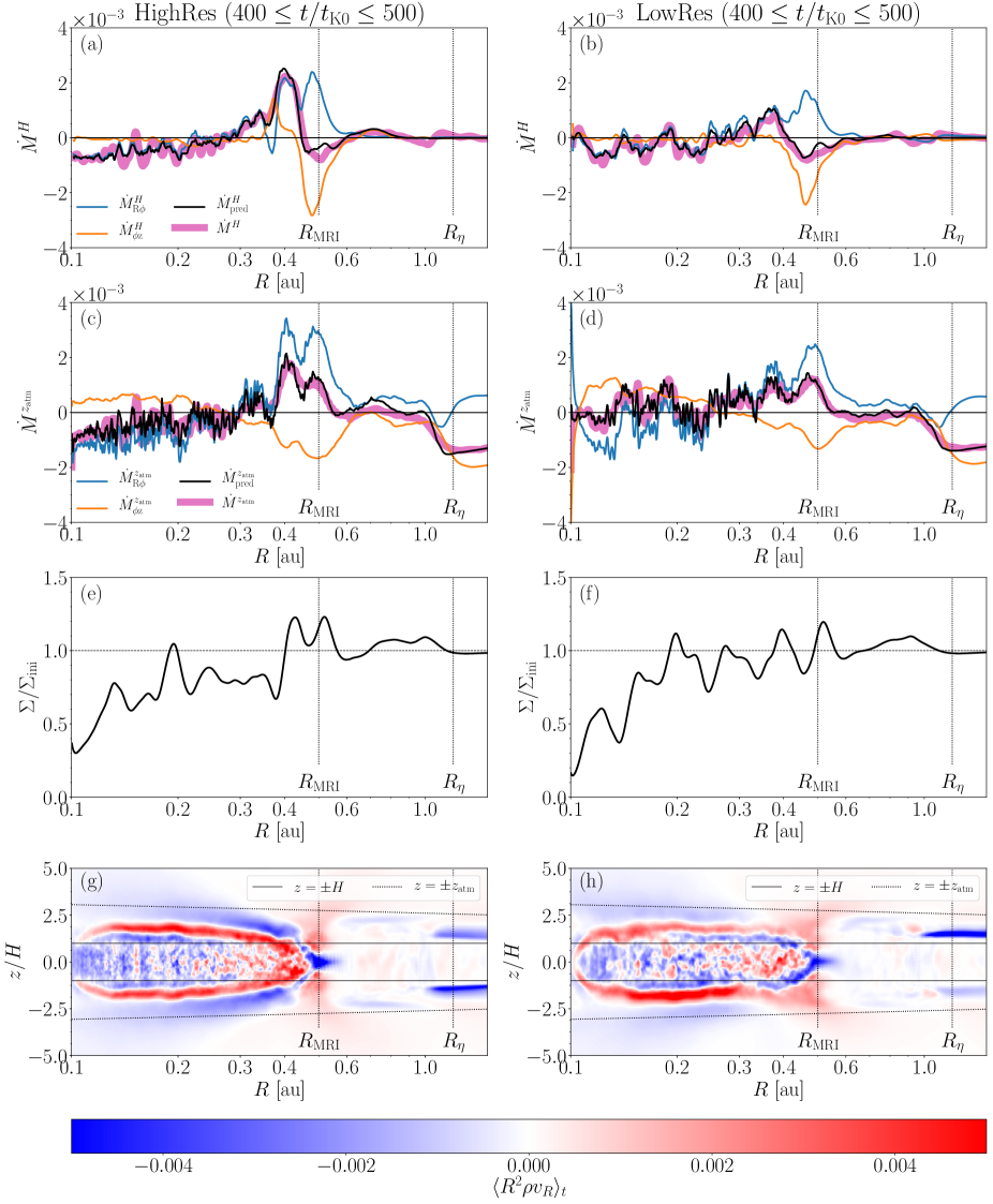
Figure 23: Radial dependence of the mass accretion rate in the early stage for HighRes (left) and LowRes (right). All the quantities shown in this figure are averaged over $400t_{\mathrm{K0}}\leq t\leq 500t_{\mathrm{K0}}$. The first row compares the mass accretion rate (pink) integrated over $|z|\leq H$ and their predictions (black) given by Equation (53). The blue and orange lines correspond to $\dot{M}_{R\phi}^{H}$ and $\dot{M}_{\phi z}^{H}$, respectively. The second row is the same as the first row but the mass accretion rate is integrated over $|z|\leq z_{\mathrm{atm}}$. The radial profiles of the surface densities are shown in the third row. In the fourth row, the color maps of $R^{2}\langle\rho v_{R}\rangle_{t}$ are displayed in the plane of ($\log_{10}R,z/H$), and the black solid and dashed lines correspond to $z=\pm H$ and $z=\pm z_{\mathrm{atm}}$. In each panel, the two vertical dotted lines show $R=R_{\mathrm{MRI}}$ and $R=R_{\eta}$. In the first and second row, to reduce significant spatial fluctuations of the mass accretion rates $\dot{M}_{R\phi}^{H,z_{\mathrm{atm}}}$, $\dot{M}_{\phi z}^{H,z_{\mathrm{atm}}},\dot{M}_{\mathrm{pred}}^{H,z_{\mathrm{atm}}}$, the centered moving averages over $\Delta R/R=0.4$ are taken. All the quantities are shown in the code units.

4.1.1 Early Evolution

First, we investigate the angular momentum transfer in the early evolution $400t_{\mathrm{K0}}\leq t\leq 500t_{\mathrm{K0}}$. The simulation time is long enough for the turbulence in the active zone to reach saturation (Figure 36), but not long enough to capture the secular evolution, such as the ring formation and flux concentration (Figure 11). At $R=R_{\eta}$, the gas rotates only 14 rotations at $t=450t_{\mathrm{K0}}$, indicating that both the transition and coherent zones have not reached quasi-steady states. In this section, we investigate the angular momentum transport mechanism especially in the active zone and around the inner edge of the transition zone.

The top and second rows of Figure 23 show comparison between the measured and predicted mass accretion rates by integrating over $|z|\leq H$ and $|z|\leq z_{\mathrm{atm}}$, respectively. Equation (53) reproduces the actual mass accretion rates reasonably well for all the panels.

Next, we investigate the mass transfer in the active zone around the mid-plane ($|z|\leq H$). Figures 23a and 23b show that the mass transfer is mainly driven by the $R\phi$ torque due to the MRI turbulence while the contribution from the $\phi z$ torque is negligible. The active zone shows that the radial mass fluxes are negative at $R\lesssim 0.25~{}$au while they are positive in the outer region. This is a typical feature of viscous evolution of an isolated accretion disk where the outer region expands outward by receiving the angular momentum from the inner region where the gas accretes inwards. The resolution dependence of the radial mass flux is seen especially in the expanding outer region ($0.25~{}\mathrm{au}\lesssim R\lesssim R_{\mathrm{MRI}}$). The outward radial mass flux around $R\sim 0.4~{}\mathrm{au}$ is more significant in HighRes than in LowRes run.

When the upper layers of the disk is considered in the estimation of the mass accretion rate, the resolution dependence becomes more significant. For HighRes run, the mass accretion rate is not influenced by the upper layers significantly, or $\dot{M}^{H}\sim\dot{M}^{z_{\mathrm{atm}}}$ (Figures 23a and 23c). By contrast, LowRes run shows that $\langle W_{\phi z}\rangle$ owing to large-scale magnetic fields in the upper layers makes $\dot{M}_{z_{\mathrm{atm}}}$ positive in the inner active zone although $\dot{M}^{H}$ is negative there. The corresponding structure in Figure 23h is the outgoing gas upper layers in the active zone. This is because the magnetic fields are more coherent for LowRes run than HighRes run.

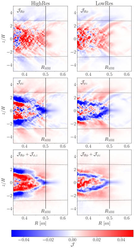
Figure 24: Color maps of ${\cal J}_{R\phi}$, ${\cal J}_{\phi z}$, and ${\cal J}_{R\phi}+{\cal J}_{\phi z}$ averaged over $400t_{\mathrm{K0}}\leq t\leq 500t_{\mathrm{K0}}$ for HighRes (left panels) and LowRes runs (right panels). The dotted lines correspond to $z=\pm z_{\mathrm{atm}}$, respectively. All the quantities are shown in the code units.

Next, we investigate the mass transfer around the inner edge of the transition zone. Since the angular momentum transfer mechanisms change significantly both radially and vertically, it is unclear which heights of the gas mainly contribute to $\dot{M}_{R\phi}$ and $\dot{M}_{\phi z}$ at a given radius only from the first and second rows of Figure 23. The color maps of the integrands of $\dot{M}_{R\phi}$ and $\dot{M}_{\phi z}$, or ${\cal J}_{R\phi}$ and ${\cal J}_{\phi z}$ (see Equations (54) and (55)) are displayed in Figure 24.

The bottom rows of Figures 23 and 24, or the distributions of $\langle\rho v_{R}\rangle$ and ${\cal J}_{R\phi}+{\cal J}_{\phi z}$, look quite similar, showing that the radial mass flux is determined by the local torque acting on the gas. Interestingly, Figure 24 shows that small-scale substructures in ${\cal J}_{R\phi}$ and ${\cal J}_{\phi z}$ have complementary spatial distributions to each other, and their sum has a much smoother distribution.

As explained in Section 3.2.2, the hourglass-shaped magnetic field with a steep gradient of $B_{\phi}$ at the mid-plane is generated mainly by AD (Figure 14b). The middle row of Figures 24 clearly shows that the $\phi z$ stress drives gas accretion at the mid-plane. By contrast, the outflows just above the mid-plane accreting layer identified in the bottom row of Figure 23 are driven by the $R\phi$ stress.

From Figures 23a and 23b, it is found that the gas within $|z|\leq H$ moves inward around $R=R_{\mathrm{MRI}}$ because the gas accretion rate due to ${\cal J}_{\phi z}$ dominates over the outflow rate due to ${\cal J}_{R\phi}$. When the contribution of the upper layers ($H\leq|z|\leq z_{\mathrm{atm}}$) is taken into account, the net mass flux $\dot{M}^{z_{\mathrm{atm}}}$ is directed outward (Figures 23c and 23d), leading to the mass supply from the active zone to the transition zone (Section 4.2).

As one moves inward from $R=R_{\mathrm{MRI}}$, the layer with ${\cal J}_{\phi z}<0$ is divided into two layers that sandwitch the active zone in between (the middle row of Figure 24). Inside the active zone, the $R\phi$ stress moves the gas outward. Just above the two accreting layers, the outflows are driven mainly by the $\phi z$ stress, although the $R\phi$ stress also contributes.

The surface density radial profiles are shown in Figures 23e and 23f. Roughly speaking, the gas is accumulated around the inner-edge of the transition zone by outward turbulent diffusion in the outer region of the active zone. Looking more closely at the inner edge of the transition zone in Figure 23e, there are two density peaks around $R\sim 0.43~{}\mathrm{au}$ and $R\sim 0.52~{}\mathrm{au}$ for HighRes run. The inner peak is formed by the viscous expansion of the active zone while the outer peak is formed by the wind launched around the inner-edge of the transition zone (Section 3.2.2). The gap between the two peaks is located at the boundary between the expanding layer due to the MRI turbulence and the mid-plane accreting layer (Figure 23h). For LowRes run, the inner density peak is slightly closer to the central star than for HighRes run since the outward radial mass flux around $R\sim 0.4~{}\mathrm{au}$ is smaller for LowRes run (Figures 23c and 23d).

4.1.2 Later Evolution

Figure 25 is the same as Figure 23 but showing the late evolution for LowRes run. In the active zone, as shown in Section 3.2.1, the ring structures and flux concentrations develop.

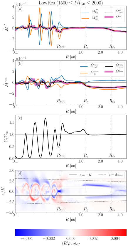
Figure 25: The same as Figure 23 but the quantities are averaged over $1500\leq t/t_{\mathrm{K0}}\leq 2000$ for LowRes run. In Panels (a) and (b), to reduce significant spatial fluctuations of the mass accretion rates $\dot{M}_{R\phi}^{H,z_{\mathrm{atm}}}$, $\dot{M}_{\phi z}^{H,z_{\mathrm{atm}}},\dot{M}_{\mathrm{pred}}^{H,z_{\mathrm{atm}}}$, the centered moving averages over $\Delta R/R=0.4$ are taken. All the quantities are shown in the code units.

Unlike in the early evolution, the outer regions of the active zone ($R\sim 0.4~{}\mathrm{au}$) do not show outward mass flux $\dot{M}^{H}>0$ and $\dot{M}^{z_{\mathrm{atm}}}>0$ in the long-term evolution (Figures 25a and 25b). The net gas accretion flows through the disk with $|z|\leq H$ and $|z|\leq z_{\mathrm{atm}}$ are almost zero. One can identify the gas flow converging to the rings both in Figures 25a and 25b. As will be shown in Section 4.2.1, gas accretion in higher latitudes to the inner boundary continues in the late evolution.

The behaviors around the inner edge of the transition zone shown in Figure 25 are similar to those shown in Figure 23. Inside the disk ($R\sim R_{\mathrm{MRI}}$, $|z|\leq H$), the mass is transferred inward by the $\phi z$ torque due to the hour-glass-shaped magnetic fields. When the upper layers of the disk ($|z|\leq z_{\mathrm{atm}}$) is considered, the inward angular momentum transfer is almost compensated by the outward angular momentum transfer owing to the $R\phi$ torque. In Section 4.2, we will see that the absence of net angular momentum transport around the inner edge of the transition zone results in almost zero radial mass transfer from the active zone to the transition zone (Figure 26).

For $R_{\eta}\leq R\lesssim R_{\mathrm{ch}}$, surface gas accretion flows are seen in $H<|z|<z_{\mathrm{atm}}$ in Figure 25d. The surface gas accretion flows are anti-symmetric with respect to the mid-plane because the current sheet is not at the mid-plane but at the lower AD dead-zone boundary (see Figure 7c). Figures 25a and 25b show that this accretion flow is driven by the magnetic braking owing to the coherent magnetic field ($\langle W\rangle_{\phi z}$). Since the outer region of the transition zone does not have gas accretion, the gas is accumulated around $R=R_{\eta}$ (Figure 25c).

The mass accretion rate in the coherent zone is determined by $\langle W_{\phi z}\rangle$. Using the ratio $f_{\phi z}=B_{\phi}/B_{z}$ and Equation (55), the mass accretion rate driven by magnetic braking is estimated to be

$$\dot{M}=\frac{8\pi R}{\Omega_{\mathrm{K}}}\frac{f_{\phi z}B_{z}^{2}}{4\pi}=2\pi R\Sigma c_{\mathrm{s,mid}}\times\left(4\sqrt{2/\pi}f_{\phi z}\beta_{z}^{-1}\right),$$ (57)

where $\beta_{z}=8\pi\rho_{\mathrm{mid}}c_{\mathrm{s,mid}}^{2}/B_{z}^{2}$. Equation (57) predicts that $\dot{M}\sim 10^{-3}$ in the code units at $R=1~{}\mathrm{au}$ and $\dot{M}$ decreases in proportion to $\propto R^{-1/4}$ since $\Sigma\propto R^{-1}$ (Equation (5)), where we use the fact that the radial magnetic flux transport from the transition zone decreases $\beta_{z}$ in the coherent zone by a factor of two from the initial plasma beta $10^{4}$ (Section 3.2.3) and $f_{\phi z}$ is estimated to $\sim 5$ from the simulation result.

Beyond $R\sim R_{\mathrm{ch}}$, the surface gas accretion flows disappear and mid-plane gas accretion is driven by the magnetic torque exerted at the mid-plane (Figures 25a and 25d) since $\eta_{\mathrm{O}}$ becomes small enough for the toroidal field to be amplified inside the disk (Figure 8c).

4.2 Time Evolution of the Masses of the Three Zones

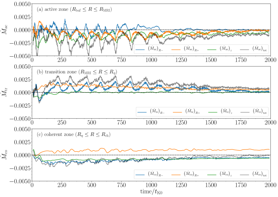
Figure 26: Mass transfer rate through the four surfaces of (a) the active, (b) transition, and (c) coherent zones for LowRes run. The blue, orange, and green lines correspond to $\left(\dot{M}_{\mathrm{ac,tr,co}}\right)_{R+}$, $\left(\dot{M}_{\mathrm{ac,tr,co}}\right)_{R-}$, and $\left(\dot{M}_{\mathrm{ac,tr,co}}\right)_{z}$, respectively. The gray lines show $\left(\dot{M}_{\mathrm{ac,tr,co}}\right)_{\mathrm{tot}}$. To reduce significant temporal fluctuations of the mass transfer rates, we take the $20t_{\mathrm{K0}}$ centered moving average for them. All the quantities are shown in the code units.

In this section, we investigate how much mass is transferred between the active, transition, and coherent zones and is ejected from or falls onto the disk in the vertical directions.

We measure the mass fluxes passing through surfaces enclosing each of the active, transition, and coherent zones. In each zone, the inner and outer radii are denoted by $R_{-}$ and $R_{+}$, respectively ( $R_{-}=R_{\mathrm{buf}}$ and $R_{+}=R_{\mathrm{MRI}}$ for the active zone, $R_{-}=R_{\mathrm{MRI}}$ and $R_{+}=R_{\eta}$ for the transition zone, and $R_{-}=R_{\eta}$ and $R_{+}=R_{\mathrm{ch}}$ for the coherent zone). The upper and lower boundaries in the vertical directions are $z=+z_{\mathrm{atm}}(R)$ and $z=-z_{\mathrm{atm}}(R)$, respectively.

The time evolution of the total masses of the active, transition, and dead zones is given by

$$(\dot{M}_{\mathrm{ac,tr,co}})_{\mathrm{tot}}=(\dot{M}_{\mathrm{ac,tr,co}})_{R+}+(\dot{M}_{\mathrm{ac,tr,co}})_{R-}+(\dot{M}_{\mathrm{ac,tr,co}})_{z},$$ (58)

where the subscripts ”ac”, ”tr”, and ”co” stand for the active, transition, and coherent zones, respectively, the mass increasing rates passing through the surfaces $R=R_{-}$ and $R_{+}$ are denoted by $(\dot{M}_{\mathrm{ac,tr,co}})_{R-}$ and $(\dot{M}_{\mathrm{ac,tr,co}})_{R+}$, respectively, and the mass increasing rates from the surfaces $z=-z_{\mathrm{atm}}$ and $z=+z_{\mathrm{atm}}$ are added and denoted as $(\dot{M}_{\mathrm{ac,tr,co}})_{z}$. The signs of $(\dot{M}_{\mathrm{ac,tr,co}})_{R-}$, $(\dot{M}_{\mathrm{ac,tr,co}})_{R+}$, and $(\dot{M}_{\mathrm{ac,tr,co}})_{z}$ are determined so that they are positive when the total mass inside the enclosed region increases owing to its contribution. Since the surface at $R=R_{\mathrm{MRI}}$ ($R=R_{\eta}$) is shared between the active and transition zones (the transition and coherent zones), $(\dot{M}_{\mathrm{ac}})_{R+}=-(\dot{M}_{\mathrm{tr}})_{R-}$ ($(\dot{M}_{\mathrm{tr}})_{R+}=-(\dot{M}_{\mathrm{co}})_{R-}$) is satisfied. Figure 26 shows the time evolution of $(\dot{M}_{\mathrm{ac,tr,co}})_{R+}$, $(\dot{M}_{\mathrm{ac,tr,co}})_{R-}$ , $(\dot{M}_{\mathrm{ac,tr,co}})_{z}$, and $(\dot{M}_{\mathrm{ac,tr,co}})_{\mathrm{tot}}$.

4.2.1 The Active Zone

Figure 26a shows that $(\dot{M}_{\mathrm{ac}})_{\mathrm{tot}}$ is always negative, indicating that the total mass of the active zone decreases with time. The time evolution of $(\dot{M}_{\mathrm{ac}})_{R-}$, $(\dot{M}_{\mathrm{ac}})_{R+}$, and $(\dot{M}_{\mathrm{ac}})_{z}$ can be divided into the early and late phases. The former shows quasi-periodic oscillations and the latter is characterized by quasi-steady state (Figure 37). The late phase corresponds to the development of the ring structures.

In the early phase ($t\lesssim 1300~{}t_{\mathrm{K0}}$), the mass of the active zone is lost both vertically and radially with significant time variations. In the radial directions, the mass of the active zone flows out more from $R=R_{+}=R_{\mathrm{MRI}}$ than from $R=R_{-}=R_{\mathrm{buf}}$. The mass ejection rate by the disk wind $(\dot{M}_{\mathrm{ac}})_{z}$ is comparable to $(\dot{M}_{\mathrm{ac}})_{R+}$. The mass transport rate through $R=R_{+}$ is investigated in Section 4.2.2 in detail. This indicates that the vertical mass loss is as important as the radial mass transport.

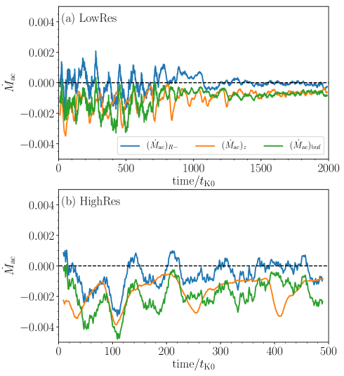
Figure 27: Mass transfer in the active zone. Time evolution of $(\dot{M}_{\mathrm{ac}})_{R-}$, $(\dot{M}_{\mathrm{ac}})_{z}$, and $(\dot{M}_{\mathrm{ac}})_{\mathrm{buf}}$ for (a) LowRes and (b) HighRes runs. To reduce significant temporal fluctuations of the mass transfer rates, we take the $20t_{\mathrm{K0}}$ centered moving average for them. All the quantities are shown in the code units.

In the later phase ($t\gtrsim 1300~{}t_{\mathrm{K0}}$), $(\dot{M}_{\mathrm{ac}})_{R-}$ and $(\dot{M}_{\mathrm{ac}})_{R+}$ approach zero. The vertical mass flow mainly removes the mass of the active zone. Where does the mass ejected vertically from $z=\pm z_{\mathrm{atm}}(R)$ go? Since the radial velocity in $|z|>z_{\mathrm{atm}}$ above the active zone is negative (the bottom panels of Figure 23 and Figure 25), the disk wind falls onto the center. In order to take into account mass accretion at high latitudes at $R=R_{\mathrm{buf}}$, we measure the mass accretion rate $(\dot{M}_{\mathrm{ac}})_{\mathrm{buf}}$ through the sphere $r=R_{\mathrm{buf}}$, where we take into account only the regions where $\rho>10^{-2}$ to remove the funnel regions. Figure 27 shows that $(\dot{M}_{\mathrm{ac}})_{\mathrm{buf}}$ is comparable to $(\dot{M}_{\mathrm{ac}})_{z}$ in all the times for LowRes and HighRes runs. This indicates that most mass ejected vertically falls onto the center (Takasao et al., 2018).

4.2.2 The Transition Zone

The mass flux from the active zone to the transition zone $(\dot{M}_{\mathrm{tr}})_{R-}=(\dot{M}_{\mathrm{ac}})_{R+}$ shows significant quasi-periodic time variations in the early phase of $t\lesssim 1300t_{\mathrm{K0}}$; time periods with large and small $(\dot{M}_{\mathrm{tr}})_{R-}$ are periodically repeated. The rate of the mass supply passing through $R=R_{-}=R_{\mathrm{MRI}}$ is positive most of the time. This is consistent with the mass transfer rate shown in Figures 23. The time variability of $(\dot{M}_{\mathrm{tr}})_{R-}$ is attributed to the MRI activity in the active zone. For $t\gtrsim 1300t_{\mathrm{K0}}$, the quasi-periodic time variations in $(\dot{M}_{\mathrm{tr}})_{R-}$ disappear and $(\dot{M}_{\mathrm{tr}})_{R-}$ gradually decreases with time. This corresponds to the decrease in the MRI activity in the active zone shown in Figure 37.

Figure 26b shows that the mass transfer rate $(\dot{M}_{\mathrm{tr}})_{R+}$ is positive and does not show a significant time variation. This is consistent with the fact that the gas is transferred from the dead zone to the transition zone by the quasi-steady surface accretion flow.

Figure 28: Vertical mass outflow rate from $R$ to $R+dR$ as a function of radius. Panel (a) compares the results for LowRes and HighRes, and they are averaged over $400\leq t/t_{\mathrm{K0}}\leq 500$. Panel (b) displays the time evolution of $d\dot{M}_{\mathrm{wind}}/d\ln R$ by showing the result averaged over three different time intervals, $500\leq t/t_{\mathrm{K0}}\leq 1000$, $1000\leq t/t_{\mathrm{K0}}\leq 1500$, and $1500\leq t/t_{\mathrm{K0}}\leq 2000$. The gas accretion rate in the coherent zone is shown by the magenta line. All the quantities are shown in the code units.

Figure 26b shows that the vertical mass supply $(\dot{M}_{\mathrm{tr}})_{z}$ stays almost zero. This does not mean that there are no mass transfer at each radius. To investigate the radial profile of the mass ejection rate by the disk wind, in Figure 28 we plot the mass ejection rate from the surfaces of $z=\pm z_{\mathrm{atm}}$ from $R$ to $R+dR$ that is given by

$$\frac{d\dot{M}_{\mathrm{wind}}}{d\ln R}=2\pi R^{2}\left[(\langle\rho v_{n}\rangle)_{z_{\mathrm{atm}}}+(-\langle\rho v_{n}\rangle)_{-z_{\mathrm{atm}}}\right],$$ (59)

where the gas is ejected from the surfaces of $z=\pm z_{\mathrm{atm}}$ when $d\dot{M}_{\mathrm{wind}}/d\ln R>0$. Figure 28 shows that the mass is lost in $R_{\mathrm{MRI}}\leq R\leq 0.6~{}\mathrm{au}$ and is supplied in the outer region. This profile can be understood by the velocity field above the transition zone. Most amount of the gas outflowing from the inner part falls back within the transition zone owing to the failed disk wind (Figure 13f).

4.2.3 The Coherent Zone

Unlike the active and transition zones, the change rate of the coherent zone mass ($R_{\eta}\leq R\leq R_{\mathrm{ch}}$) appears to approach zero in the long-term evolution (Figure 26c). The mass supply through $R=R_{+}=R_{\mathrm{ch}}$ almost balances with the mass loss through $R=R_{-}=R_{\eta}$ and disk wind. We note that our calculation time may not be long enough for $(\dot{M}_{\mathrm{co}})_{R+}$ to reach a quasi-steady state. About half of the mass supplied through $R=R_{+}=R_{\mathrm{ch}}$ is ejected by the disk wind, and the remaining half is transferred to the transition zone since $(\dot{M}_{\mathrm{co}})_{z}\sim(\dot{M}_{\mathrm{co}})_{R-}$ (Figure 26c).

Ferreira (1997) defines ”the ejection index” as

$$\xi\equiv\frac{d\dot{M}_{\mathrm{wind}}/d\ln R}{\dot{M}^{z_{\mathrm{atm}}}},$$ (60)

which indicates a mass ejection efficiency because $\dot{M}_{\mathrm{wind}}$ obtained from the radial integration of $d\dot{M}_{\mathrm{wind}}/d\ln R$ increases more rapidly compared with the accretion rate $\dot{M}^{z_{\mathrm{atm}}}$ as the radial extent considered in the integration for larger $\xi$.

Figure 28b shows that $\dot{M}^{z_{\mathrm{atm}}}\sim d\dot{M}_{\mathrm{wind}}/d\ln R$, indicating that significant mass loss occurs in our simulations. The ejection index is about unity, or $\xi\sim 1$ (Equation (60)). By the angular momentum conservation and the induction equation, $\xi$ and the magnetic lever arm $\lambda\equiv(R_{\mathrm{A}}/R_{0})^{2}$ are related, where $R_{0}$ is the radius at a radius where the disk wind is launched and $R_{\mathrm{A}}$ is the Alfvén radius of the radius, or $\xi=\left[2\left(\lambda-1\right)\right]^{-1}$ (Pelletier & Pudritz, 1992). From the fact that $\xi\sim 1$, the magnetic lever arm is estimated to $\lambda\sim 1.5$. The lever arm is much shorter than expected in a typical magneto-centrifugal wind (Ferreira, 1997). Disk winds with short lever arms were reported; $\lambda\sim 1.4$ (Béthune et al., 2017) and $\lambda\sim 1.15$ (Bai, 2017).

Bai et al. (2016) pointed out the wind kinematics is mainly controlled by the plasma beta around the wind base. Supposing that the wind base is at $z=z_{\mathrm{atm}}$, the plasma beta is $\beta_{0}\times\exp(-(z_{\mathrm{atm}}/H)^{2})\sim 20$. For such a high $\beta$, the magneto-centrifugal winds (Blandford & Payne, 1982) do not occur since the magnetic fields are too weak to corotate with the Kepler rotation at the wind base within the Alfvén radius. Instead, the thermal and magnetic pressure gradient forces accelerate the winds with the short lever arm $\lambda\sim 1.5$.

4.3 Magnetic Flux Transport

We define the following two kinds of the magnetic fluxes. One is the magnetic flux threading the northern hemisphere at a given radius $r$ that is given by

$$\Psi_{\mathrm{rad}}(r)=\int_{0}^{\pi/2}\sin\theta d\theta\int_{0}^{2\pi}d\phi r^{2}B_{r}(r,\theta,\phi).$$ (61)

The other is the magnetic flux threading the mid-plane from $R=r_{\mathrm{in}}$ to $R$,

$$\Psi_{\mathrm{mid}}(R)=\int_{r_{\mathrm{in}}}^{R}RdR\int_{0}^{2\pi}d\phi B_{z}(r,\theta,\phi).$$ (62)

The divergence-free condition in the northern hemisphere gives

$$\Psi_{\mathrm{rad}}(r)=\Psi_{\mathrm{rad}}(r_{\mathrm{in}})+\Psi_{\mathrm{mid}}(R).$$ (63)

where $R$ is identical to $r$ at $\theta=\pi/2$, because all the magnetic field lines passing through the northern hemisphere at the inner edge and the mid-plane from $R=r_{\mathrm{in}}$ to $R$ penetrate through the northern hemisphere at $r$.

From Equation (63), one obtains

$$\Psi_{\mathrm{rad}}(r_{\mathrm{out}})=\Psi_{\mathrm{rad}}(r_{\mathrm{in}})+\Psi_{\mathrm{mid}}(R_{\mathrm{out}}),$$ (64)

where $R_{\mathrm{out}}=r_{\mathrm{out}}$ is the outermost cylindrical radius of the simulation box. Equation (64) shows how the total magnetic flux $\Psi_{\mathrm{rad}}(r_{\mathrm{out}})$ is distributed between $\Psi_{\mathrm{rad}}(r_{\mathrm{in}})$ and $\Psi_{\mathrm{mid}}(R_{\mathrm{out}})$.

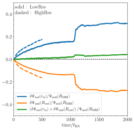
Figure 29: Time Evolution of $\Psi_{\mathrm{rad}}(r_{\mathrm{in}})$, $\Psi_{\mathrm{mid}}(R_{\mathrm{out}})$, and $\Psi_{\mathrm{rad}}(r_{\mathrm{out}})=\Psi_{\mathrm{rad}}(r_{\mathrm{in}})+\Psi_{\mathrm{mid}}(R_{\mathrm{out}})$ for LowRes (solid) and HighRes (dashed). The deviations from the respective initial values ( $\delta\Psi_{\mathrm{rad}}(r_{\mathrm{in}})$ and $\delta\Psi_{\mathrm{mid}}(R_{\mathrm{out}})$) are displayed. In addition, their values are normalized by the initial mid-plane magnetic flux within $R=R_{\mathrm{MRI}}$.

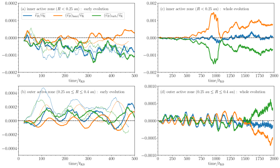
Figure 30: Time evolution of the drift velocities averaged over $R<0.25~{}$au (top) and $0.25~{}\mathrm{au}\leq R\leq 0.4~{}\mathrm{au}$ (bottom) for LowRes. The left and right panels show the early and whole evolution, respectively. For comparison, the results for HighRes are shown by the thin dashed line in the left panels. In each panel, $\left(\widetilde{v_{\mathrm{B}}}\right)_{\mathrm{lami}}$, $\left(\widetilde{v_{\mathrm{B}}}\right)_{\mathrm{turb}}$, and $\left(\widetilde{v_{\mathrm{B}}}\right)$ are shown, and are normalized by the Kepler speed $\widetilde{v_{\mathrm{K}}}$ averaged over the corresponding radius range. To reduce significant temporal fluctuations of the drift velocities, we take the $20t_{\mathrm{K0}}$ centered moving average for them.

The time evolution of $\Psi_{\mathrm{rad}}(r_{\mathrm{in}})$ and $\Psi_{\mathrm{mid}}(R_{\mathrm{out}})$ is shown in Figure 29. Because $\Psi_{\mathrm{mid}}(R_{\mathrm{out}})$ is much larger than $\Psi_{\mathrm{rad}}(r_{\mathrm{in}})$ at the initial condition, Figure 29 displays the deviations from the respective initial values, $\delta\Psi_{\mathrm{rad}}(r_{\mathrm{in}})$ and $\delta\Psi_{\mathrm{mid}}(R_{\mathrm{out}})$. In addition, their values are normalized by the initial mid-plane magnetic flux within $R=R_{\mathrm{MRI}}$. Figure 29 shows that $\Psi_{\mathrm{rad}}(r_{\mathrm{in}})$ increases with time while $\Psi_{\mathrm{mid}}(R_{\mathrm{out}})$ decreases with time, keeping $\Psi_{\mathrm{rad}}(r_{\mathrm{in}})+\Psi_{\mathrm{mid}}(R_{\mathrm{out}})$ almost constant. This clearly shows that the magnetic fluxes passing through the mid-plane accrete onto the inner edge. Comparison between the results of LowRes and HighRes shows that the magnetic flux accretes onto the inner boundary more rapidly for HighRes than for LowRes run.

The increasing rate of $\Psi_{\mathrm{rad}}(r_{\mathrm{in}})$ decreases with time except for a sudden increase around $t=1000t_{\mathrm{K0}}$, which corresponds to the accretion of the innermost $\langle B_{z}\rangle$ concentration onto the inner boundary of the simulation box around $t=1000t_{\mathrm{K0}}$ (Figure 19). In the late evolution ($1500t_{\mathrm{K0}}\leq t\leq 2000t_{\mathrm{K0}}$), the magnetic flux at the inner boundary hardly changes while the gas accretion onto the inner boundary continues (Figure 27). This decrease in the increasing rate of $\Psi_{\mathrm{rad}}(r_{\mathrm{in}})$ has been reported in Beckwith et al. (2009) and Takasao et al. (2018).

In Sections 4.3.1, 4.3.2, and 4.3.3, we will investigate the radius dependence of the magnetic flux transport in the active, transition, and coherent zones, respectively. The trajectories of the magnetic flux are shown by the contours of $\Psi_{\mathrm{rad}}$ shown in Figure 19. It is clearly seen that the behaviors of the magnetic field transport are different between the three zones. We define a drift speed of the magnetic flux $v_{\mathrm{B}}$ as follows:

$$\langle v_{B}\rangle\equiv{\langle E_{\phi}\rangle}/{\langle B_{z}\rangle}$$ (65)

(Guilet & Ogilvie, 2012; Bai & Stone, 2017).

4.3.1 The Active Zone

The trajectories of the magnetic flux and the color map of $\langle B_{z}\rangle_{H}$ in Figure 19a show that the flux concentrations become prominent for $t\gtrsim 500t_{\mathrm{K0}}$, and the contours of $\Psi_{\mathrm{rad}}$ converges to the multiple $\langle B_{z}\rangle$ concentrations.

First we investigate the magnetic flux transport before developing the flux concentrations. We divide the active zone into two regions, the inner region with $R<0.25~{}\mathrm{au}$ and the outer region with $0.25~{}\mathrm{au}\leq R\leq 0.4~{}\mathrm{au}$ because the magnetic flux moves inward at $R<0.25~{}\mathrm{au}$. The outermost radius is set to $R=0.4~{}\mathrm{au}$ because beyond $R=0.4~{}\mathrm{au}$ the MRI turbulence is affected by OR (Figure 35). In each of the inner and outer regions, we average $\langle v_{B}\rangle$ in the radial direction as follows:

$$\widetilde{v_{B}}\equiv\int 2\pi R\langle(E_{\phi})_{\mathrm{I}}\rangle_{H}dR\times\left(\int 2\pi R\langle B_{z}\rangle_{H}dR\right)^{-1}.$$ (66)

In order to investigate what determines the drift speed, we decompose $\langle({E}_{\phi})_{\mathrm{I}}\rangle_{H}=\langle v_{R}B_{z}\rangle_{H}-\langle v_{z}B_{R}\rangle_{H}$ into the laminar component

$$\left(\langle({E}_{\phi})_{\mathrm{I}}\rangle_{H}\right)_{\mathrm{lami}}=\langle v_{R}\rangle_{H,v}\langle B_{z}\rangle_{H}-\langle v_{z}\rangle_{H,v}\langle B_{R}\rangle_{H},$$ (67)

and the turbulent component

$$\left(\langle({E}_{\phi})_{\mathrm{I}}\rangle_{H}\right)_{\mathrm{turb}}=\langle(v_{R}-\langle v_{R}\rangle_{H,v})\delta B_{z}\rangle_{H}-\langle(v_{z}-\langle v_{z}\rangle_{H,v})\delta B_{R}\rangle_{H},$$ (68)

where $\langle(E_{\phi})_{\mathrm{I}}\rangle_{H}=\left(\langle(E_{\phi})_{\mathrm{I}}\rangle_{H}\right)_{\mathrm{lami}}+\left(\langle(E_{\phi})_{\mathrm{I}}\rangle_{H}\right)_{\mathrm{turb}}$ is satisfied. Although the mass-weighted average is taken when we calculate the mean values of the velocity in Section 2.7, the volume-weighted average should be applied for the velocity when the flux transport is discussed. To distinguish the volume-weighted mean velocity, the subscript ”$v$” is used, or $\langle v_{R,z}\rangle_{H,v}$. The radially-averaged drift velocities originating from the laminar and turbulent components of $\langle(E_{\phi})_{\mathrm{I}}\rangle$ are defined by replacing $\langle(E_{\phi})_{\mathrm{I}}\rangle_{H}$ with $\left(\langle(E_{\phi})_{\mathrm{I}}\rangle_{H}\right)_{\mathrm{lami}}$ and $\left(\langle(E_{\phi})_{\mathrm{I}}\rangle_{H}\right)_{\mathrm{turb}}$ in Equation (66), and are denoted by $(\widetilde{v_{\mathrm{B}}})_{\mathrm{lami}}$ and $(\widetilde{v_{\mathrm{B}}})_{\mathrm{turb}}$, respectively.

In the early evolution ($t\leq 500~{}t_{\mathrm{K0}}$), the magnetic flux moves inward in the inner active zone $(R<0.25~{}\mathrm{au})$ and moves outward in the outer active zone $(0.25~{}\mathrm{au}\geq R\leq 0.4~{}\mathrm{au})$ as shown in Figures 30a and 30b which display the time evolution of $\widetilde{v_{\mathrm{B}}}$ and the contributions from the laminar and turbulent components. In the inner active zone, the turbulent $(E_{\phi})_{\mathrm{I}}$ mainly drives inward drift of the magnetic flux at a speed of $\sim 5\times 10^{-5}v_{\mathrm{K}}$. Although the resolution dependence of $\widetilde{v_{\mathrm{B}}}$ is found in $t\leq 300~{}t_{\mathrm{K0}}$, it disappears in $300\lesssim t/t_{\mathrm{K0}}\lesssim 500$.

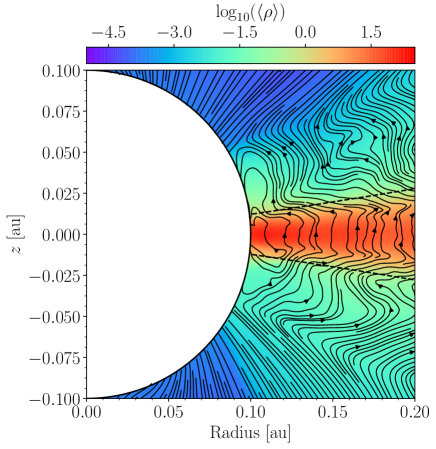
Figure 31: Poloidal magnetic fields structure near the inner boundary at $t=500t_{\mathrm{K0}}$. The color map shows $\log_{10}\langle\rho\rangle$, and the streaming lines show the poloidal magnetic fields averaged over $0\leq\phi<2\pi$. The two dashed lines correspond to $z=\pm z_{\mathrm{atm}}$. The densities are shown in the code units.

The magnetic flux transport is not determined only by the dynamics inside the disk with $|z|<H$, but is affected by the upper atmospheres. The poloidal magnetic field structures are shown in Figure 31. Just below the boundaries ($z\sim\pm 0.05~{}\mathrm{au}$ at $r=0.1~{}\mathrm{au}$) between the funnel regions and the atmospheres, the poloidal magnetic fields are dragged toward the inner boundary. After the dragged poloidal fields accrete onto the inner boundary, loop-like poloidal fields penetrating the disk form (Beckwith et al., 2009). Their edges are at the inner boundaries in the southern and northern hemispheres. When the loop poloidal fields disappear through accretion and/or magnetic reconnection, the net flux at the inner boundary $\Psi_{\mathrm{rad}}(r_{\mathrm{in}})$ increases.

In the long-term evolution in the active zone, the turbulent and laminar contributions nearly cancel each other out and their summation, or $\widetilde{v_{\mathrm{B}}}$ remains low (Figure 30c). The laminar and turbulent toroidal electric fields tend to move the magnetic flux outward and inward, respectively. The drift velocities oscillate with time and takes both positive and negative values for $t\geq 1000~{}t_{\mathrm{K0}}$, indicating that there is almost no net magnetic transport. Such a quasi-steady state has been obtained in previous global simulations (Beckwith et al., 2009; Takasao et al., 2018).

In the early evolution of the the outer active zone, outward drift of the magnetic flux is driven mainly by $\langle(E_{\phi})_{\mathrm{I}}\rangle_{\mathrm{turb}}$. Both $\langle(E_{\phi})_{\mathrm{I}}\rangle_{\mathrm{lami}}$ and $\langle(E_{\phi})_{\mathrm{I}}\rangle_{\mathrm{turb}}$ exhibit quasi-periodic oscillations whose phases are correlated with those of $\langle B_{\phi}\rangle$ oscillations in the upper atmospheres. Unlike LowRes run, HighRes run shows that the laminar component plays an important role in the outward flux transport because the outward velocity in the outer active zone is larger for HighRes than for LowRes (Figure 23a).

Figure 30d shows that the quasi-periodic oscillations continue until $t\sim 1500~{}t_{\mathrm{K0}}$ beyond which the quasi-periodic MRI activities disappear (Figure 37). Although $\widetilde{v_{\mathrm{B}}}$ is positive on average in the early phase, the net drift velocities become around zero in $500\leq t/t_{\mathrm{K0}}\leq 1000$. In addition, unlike in the inner active zone, $(\widetilde{v_{\mathrm{B}}})_{\mathrm{lami}}$ and $(\widetilde{v_{\mathrm{B}}})_{\mathrm{turb}}$ do not cancel each other out, and they oscillate in the same phase in the outer active zone. In the later phase with $t\gtrsim 1500~{}t_{\mathrm{K0}}$, $(\widetilde{v_{\mathrm{B}}})_{\mathrm{lami}}$ and $(\widetilde{v_{\mathrm{B}}})_{\mathrm{turb}}$ do not completely cancel each other out, and the magnetic flux drifts inward at $\widetilde{v_{\mathrm{B}}}\sim 10^{-4}v_{\mathrm{K}}$. The magnetic flux drifts inward at a faster speed than the gas that accretes at a speed of $\sim 10^{-6}v_{\mathrm{K}}$. Jacquemin-Ide et al. (2021) conducted a simulation (model SEp) similar to ours and obtained a drift speed consistent with our results.

4.3.2 The Transition Zone

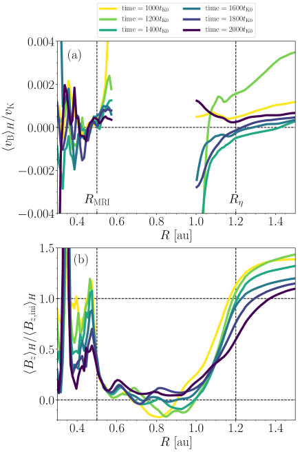
Figure 32: Time Evolution of the radial profiles of $\langle v_{\mathrm{B}}\rangle_{H}/v_{\mathrm{K}}$ and $\langle B_{z}\rangle_{H}/\langle B_{z}\rangle_{H,\mathrm{ini}}$ from $t=1000t_{\mathrm{K0}}$ to $t=2000t_{\mathrm{K0}}$. In Panel (a), we do not plot $\langle v_{\mathrm{B}}\rangle_{H}/v_{\mathrm{K}}$ in $0.6\mathrm{au}\leq R\leq 1~{}\mathrm{au}$ because scatters of the data are significant owing to almost zero $\langle B_{z}\rangle_{H}$. All the quantities are shown in the code units.

In Section 3.2.3, we found that the rapid outward transport of the magnetic flux is caused by OR and AD. In this section, we investigate the long term evolution of the magnetic flux around the transition zone. Figure 32b shows that the outer edge of the region where $\langle B_{z}\rangle_{H}\sim 0$ expands with time because the magnetic flux in the coherent zone drift outward as will be shown in Section 4.3.3. A typical drift speed of the outer edge that is identified at the radius where $\langle B_{z}\rangle_{H}=\langle B_{z,\mathrm{ini}}\rangle_{H}$ is estimated to about $10^{-3}~{}v_{\mathrm{K}}$ from Figures 32a and 32b. This drift speed is almost identical to that in the coherent zone (Figure 33).

The flux concentration around $R\sim 0.5~{}\mathrm{au}$, where a density gap exists (Figure 25c), weakens with time because $\langle v_{\mathrm{B}}\rangle_{H}$ is positive around $R\sim 0.5~{}\mathrm{au}$ (Figure 32a). Further time evolution would eliminate the flux concentration around $R\sim 0.5~{}\mathrm{au}$, resulting in inward expansion of the region where $\langle B_{z}\rangle_{H}\sim 0$. However, the inward expansion would not proceed furthermore because of rapid decreases in $\eta_{\mathrm{O}}$ and $\eta_{\mathrm{A}}$ (Figure 2).

4.3.3 The Coherent Zone

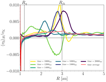
Figure 33: Time sequence of the radial profiles of the drift velocity of the magnetic flux $\langle v_{\mathrm{B}}\rangle_{H}$ normalized by the Kepler speed from $t=1000t_{\mathrm{K0}}$ to $t=2000t_{\mathrm{K0}}$. The radial profiles of $\langle v_{\mathrm{B}}\rangle_{H}$ averaged over $1000t_{\mathrm{K0}}\leq t\leq 2000t_{\mathrm{K0}}$ are shown by the red line. The vertical dashed lines correspond to $R=R_{\eta}$ and $R_{\mathrm{ch}}$ from left to right.

Figure 33 shows the time evolution of the radial profiles of $\langle v_{\mathrm{B}}\rangle_{H}/v_{\mathrm{K}}$. For $R\lesssim 3.5~{}\mathrm{au}$, although $\langle v_{\mathrm{B}}\rangle_{H}/v_{\mathrm{K}}$ is affected by the quasi-periodic disturbances from the active zone, the drift velocity is positive on average. Beyond $R\gtrsim 3.5~{}\mathrm{au}$, $\langle v_{\mathrm{B}}\rangle_{H}$ is steady. When the time average over $1000t_{\mathrm{K0}}\leq t\leq 2000t_{\mathrm{K0}}$ is taken, $\langle v_{\mathrm{B}}\rangle_{H,t}$ becomes almost constant, and is about $\langle v_{\mathrm{B}}\rangle_{H,t}\sim 10^{-3}v_{\mathrm{K}}$. This value is comparable to those in Bai & Stone (2017) and Bai (2017). Figure 34a shows that the drift velocity $v_{\mathrm{B}}=\langle E_{\phi}\rangle_{t}/\langle B_{z}\rangle_{t}$ does not depend on $z$ significantly, indicating that the magnetic fields drift outward keeping their shapes. This feature is also consistent with Bai & Stone (2017) and Bai (2017).

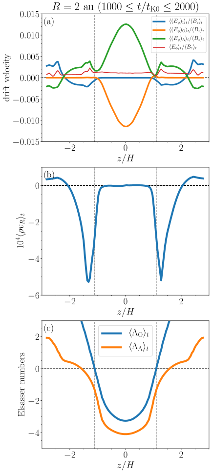
Figure 34: Vertical profiles of the quantities related to the magnetic field transport at $R=2~{}\mathrm{au}$. All the data are averaged over $1000t_{\mathrm{K0}}\leq t\leq 2000t_{\mathrm{K0}}$. (a) The vertical profiles of $\langle(E_{\phi})_{\mathrm{I}}\rangle_{t}/\langle B_{z}\rangle_{t}$, $\langle(E_{\phi})_{\mathrm{O}}\rangle_{t}/\langle B_{z}\rangle_{t}$, $\langle(E_{\phi})_{\mathrm{A}}\rangle_{t}/\langle B_{z}\rangle_{t}$, and $\langle(E_{\phi})\rangle_{t}/\langle B_{z}\rangle_{t}$. (b) The vertical profile of $\langle\rho v_{R}\rangle_{t}$. (c) The vertical profiles of $\langle\Lambda_{\mathrm{O}}\rangle_{t}$ and $\langle\Lambda_{\mathrm{A}}\rangle_{t}$. In each panel, the vertical gray dashed lines correspond to the positions where $\langle\Lambda_{\mathrm{O}}\rangle_{t}=1$. All the quantities are shown in the code units.

Since the magnetic field is almost completely decoupled with the gas inside the coherent zone where $\Lambda_{\mathrm{O}}\ll 1$ and $\Lambda_{\mathrm{A}}\ll 1$, the magnetic flux transport is determined above the coherent zone. We focus on the regions just above the OR dead zone where the surface gas accretion occurs (Figure 34b in $H\lesssim|z|\lesssim 2H$). The surface gas accretion tries to carry the magnetic flux inward since $\langle(E_{\phi})_{I}\rangle_{t}\sim\langle v_{R}B_{z}\rangle_{t}$ is negative. Diffusion due to AD, which plays an important role in the surface accretion layers ($\Lambda_{\mathrm{A}}\sim 1$), tries to drift the magnetic flux outward. Figure 34a shows that the diffusion due to AD slightly dominates over the accretion, resulting in the outward transport of the magnetic flux.

Above the surface accretion layers, the wind drags the vertical field outward ($\langle(E_{\phi})_{I}\rangle>0$). Unlike in the surface accretion layers, the diffusion due to AD is not sufficient to dominate over the wind drag because $\Lambda_{\mathrm{A}}$ increases with $z$ (Figure 34c). The drift velocity around the base of the wind ($|z|\sim 2.5H$) is close to that in the surface accretion layers.

Inside the OR dead-zone boundary ($\langle\Lambda_{\mathrm{O}}\rangle_{t}<1$), $(\langle E_{\phi}\rangle)_{\mathrm{O}}$ and $(\langle E_{\phi}\rangle)_{\mathrm{A}}$ almost cancel each other out, and the magnetic field structure inside the disk are adjusted so that $\left\{(\langle E_{\phi}\rangle)_{\mathrm{O}}+(\langle E_{\phi}\rangle)_{\mathrm{A}}\right\}/\langle B_{z}\rangle$ is comparable to the drift velocity in the region with $\Lambda_{\mathrm{O}}>1$.

5 Discussion

5.1 Structure Formation

5.1.1 The Active Zone

As shown in Figure 11, the prominent multiple rings and flux concentrations are found in the active zone. They are not transient structures but are maintained at least until $t/t_{\mathrm{K0}}=2000$. It should be noted that not all of the simulations conducted in previous studies have shown ring formation; some simulations (Bai & Stone, 2014; Hawley, 2001; Steinacker & Papaloizou, 2002; Dzyurkevich et al., 2010; Jacquemin-Ide et al., 2021) form rings and some (Suzuki & Inutsuka, 2014; Takasao et al., 2018; Zhu & Stone, 2018) do not.

In Section 3.2.1, we examined two ring formation mechanisms proposed before, the viscous instability (Suzuki, 2023) and the wind-driven instability (Riols & Lesur, 2019). The viscous instability may be a possible ring structure formation mechanism in our simulations. However, our analyses are insufficient to fully understand the ring formation in the ideal MHD. The viscous instability found in Suzuki (2023) forms transient ring structures, unlike our results. The possibility of the wind-driven instability is rejected for our simulation, but we note that our result could be affected by the inner boundary condition.

We still do not know detailed mechanisms and what determines whether multiple-rings form or not. We will address the formation of ring structures in MRI active disks by performing global simulations with a wide range of parameters in the future.

5.1.2 The Transition and Coherent Zones

Previous studies investigating the inner dead-zone edge with global non-ideal MHD simulations consider only OR (Lyra & Mac Low, 2012; Dzyurkevich et al., 2010; Flock et al., 2017). Our simulation shows that AD significantly changes the structure around the inner dead-zone edge.

Without AD, no rapid magnetic flux transport in the transition zone occurs. As shown in Section 3.2.3, if a finite $B_{z}$ exists in the initial condition, AD amplifies $\langle B_{R}\rangle$, leading to the enhancement of $\langle E_{\phi}\rangle_{\mathrm{O}}$. Since $\eta_{\mathrm{O}}$ increases rapidly with $R$ in the transition zone (Figure 2), the magnetic flux is efficiently transported outward within a few rotations at $R=R_{\mathrm{MRI}}$.

The previous studies focusing on outer disks show that AD triggers spontaneous magnetic flux concentration and form ring-like substructures in disks (Bai & Stone, 2014; Béthune et al., 2017; Suriano et al., 2018, 2019; Cui & Bai, 2021). Although the formation mechanism of the spontaneous flux concentration is still unclear, the previous papers suggest that a driving mechanism of the flux concentration is related with the fact that AD steepens the gradients of magnetic fields around magnetic nulls (Brandenburg & Zweibel, 1994). Suriano et al. (2018) found that AD generates a pinched magnetic field ($|B_{R}|\gg|B_{z}|$) at the mid-plane where the toroidal magnetic field is reversed. Then, magnetic reconnection is triggered, resulting in magnetic flux transport. Cui & Bai (2021) identified that the direction of $B_{\phi}$ is reversed in the radial direction where the magnetic flux is concentrated. Another property of AD that may form substructures in disks is that ${J_{\phi,\perp}}$ and ${J_{\phi}}$ can have opposite sign when $B_{\phi}\gg B_{R},B_{z}$. Béthune et al. (2017) pointed out AD works as anti-diffusion. This behavior is confirmed also in our simulations in Figures 21 and 34.

Although our simulations show the $B_{z}$ concentrations around the regions where the sign of $B_{\phi}$ is reversed, prominent gap structures do not form in the coherent zone. This may be caused by the $B$ dependence of $\eta_{\mathrm{A}}$. Significant flux concentrations require that $\eta_{\mathrm{A}}$ increases as $\propto B^{2}$. As shown in Figure 4, $\eta_{\mathrm{A}}$ is almost independent of $B$ for $R_{\eta}\lesssim R\lesssim R_{\mathrm{ch}}$ where the dominant negative charge carrier is dust grains. In addition to the Ohmic diffusion, this may be one of the reasons why flux concentration does not occur there.

For $R>R_{\mathrm{ch}}$, since the physical conditions are similar to those in Suriano et al. (2019), AD should generate the flux concentrations. The reason why our results do not show the flux concentrations is that the simulation time is too short for them to develop; 2000 rotations at the inner boundary corresponds to $\sim 8$ rotations at $R=4~{}\mathrm{au}$.

5.2 Implications for Long-term Evolution

Although we conducted LowRes run until $t=2000t_{\mathrm{K0}}=40~{}\mathrm{yr}$, it is much shorter than a typical disk lifetime. In this section, we discuss a lone-term evolution of the disk inferred from our results.

5.2.1 Gas Evolution

First, we consider a long-term evolution by assuming the magnetic flux is fixed. If the gas accretion rate shown in Figure 27 is maintained ($\dot{M}\sim 5\times 10^{-4}$ in the simulation unit corresponding to $\dot{M}=2.8\times 10^{-7}M_{\odot}~{}\mathrm{yr}^{-1}$), the depletion time scale of the active zone is $\sim 4\times 10^{5}~{}\mathrm{yr}$ if there is no mass supply. This may be a formation mechansim of transition disks (e.g., van der Marel, 2023).

What would be the mass transport between the transition and active zones? As discussed in Sections 3.2.2 and 4.1, the direction of the mass transfer is determined by the two competing mass flows; the mid-plane accretion and the outflow in the high latitudes. If the mass of the active zone becomes sufficiently small, the mid-plane accretion from the transition to active zone will dominate over the outflows from the active zone to the transition zone. This leads to inward mass transfer from the transition zone to the active zone.

In the coherent zone, the surface gas accretion continues to accumulate the gas in the outer edge of the transition zone. If the gas accretion rate is kept to $\dot{M}=10^{-3}$ in the simulation units (Figure 25), the mass corresponding to the initial mass of the active zone is transferred to the transition zone in $2\times 10^{5}$ yr. The accumulated gas is not directly transferred to the active zone since gas accretion inside the transition zone does not occur because of no net magnetic flux. Thus, the transferred mass forms a ring structure whose surface density contrast is about $10^{3}$ if the radial width is $\sim 0.2~{}\mathrm{au}$ at $2\times 10^{5}~{}\mathrm{yr}$. In reality, the ring will become vorticies by the Rossby-wave instability (Lovelace et al., 1999; Ono et al., 2016, 2018).

Gas accretion from the inner edge of the transition zone to the active zone may increase $R_{\mathrm{MRI}}$ when the surface density becomes low enough for cosmic rays and/or ionizing radiation to reach the mid-plane. If $R_{\mathrm{MRI}}$ gets close enough to $R_{\eta}$, the gas accumulated at the outer-edge of the transition zone may be transferred to the active zone.

5.2.2 Magnetic Flux Evolution

Existence of the transition zone significantly affect the magnetic flux evolution in PPDs. From our results, the following important conclusion can be drawn; the magnetic fluxes cannot drift from the coherent zone to the active zone.

The existence of the transition zone affects on the evolution of the active zone. The magnetic flux initially possessed by the active zone falls to the central star or is transported to the transition zone. The magnetic flux transported to the transition zone does not return to the active zone. This indicates that no magnetic flux may be supplied to the active zone from $R>R_{\mathrm{MRI}}$. If this is the case, the magnetic flux in $R\leq R_{\mathrm{MRI}}$ decreases with time, leading to a decrease in the gas accretion rates onto the central star. As the process regulates the magnetic flux accretion onto the central star, it can be important to determine magnetization of young stellar objects.

The outer-edge of the region where $B_{z}\sim 0$ moves following the drift velocity of the magnetic flux in the coherent zone as shown in Figure 32. We here define the transition zone as the region where $B_{z}\sim 0$. If $v_{\mathrm{B}}$ is positive as shown in our simulations and the previous simulations (Bai & Stone, 2017; Bai, 2017; Gressel et al., 2020), the outer edge of the transition zone moves outwards. Since the gas accretion will be suppressed in the region where $B_{z}\sim 0$, the inner-edge of the coherent zone where the surface gas accretion occurs moves outward. If $v_{\mathrm{B}}$ is negative, the outer edge of the transition zone will not move and the magnetic flux will be accumulated just outside the transition zone.

Long-term evolution of magnetic flux transport in the coherent zone remains elusive. The drift velocities have about an order of magnitude differences between the previous studies (Bai & Stone, 2017; Bai, 2017; Gressel et al., 2020). Lesur (2021) shows that the radial drift velocities strongly depend on the spatial distributions of $\eta_{\mathrm{O}}$ and $\eta_{\mathrm{A}}$ using simple self-similar solutions. Although their results show only outward drifts, we need to investigate how drift velocities depend on the disk parameters and the size distribution of dust grains. If the drift velocity can be negative in a parameter range, the magnetic flux will be accumulated at the outer edge of the transition zone. We will investigate how drift velocities depend on the disk parameters and the size of dust grains in the future.

5.3 Implication for Dynamics of Dust Grains

The inner dead-zone edge is thought to be a possible site where dust grains accumulate since a pressure bump is created owing to outward viscous expansion of the inner active zone (e.g., Kretke et al., 2009). So far, accumulation of dust grains at the inner dead-zone edge was investigated mainly by using one-dimensional (1D) model taking into account viscous evolution of disks and coupling of the gas and dust grains (Kretke et al., 2009; Pinilla et al., 2016; Ueda et al., 2019). The 1D models can compute the evolution for much longer periods than three-dimensional global disk simulations.

From our simulations considering realistic spatial distributions of $\eta_{\mathrm{O}}$ and $\eta_{\mathrm{A}}$, we found that the transition zone is created with a finite width at the inner dead-zone edge. The gas accumulates from both inner and outer edges of the transition zone, producing the two ring structures at both the edges (Figure 22a). The structure found in this study is quite different from that predicted by the 1D models that show a single pressure bump because the 1D models assume a step-function-like distribution of the viscous parameter $\alpha$ and neglect the gas surface accretion in the dead zone.

Ueda et al. (2019) derived a critical value of the $\alpha$ parameter $\alpha_{\mathrm{dead}}$ in the dead zone below which the dust pileup occurs,

$$\alpha_{\mathrm{dead}}\sim 3\times 10^{-4}\left(\frac{v_{\mathrm{frag}}}{1~{}\mathrm{m~{}s^{-1}}}\right),$$ (69)

where $v_{\mathrm{frag}}$ is the minimum collision speed that triggers fragmentation of dust grains. For silicate aggregates, $v_{\mathrm{frags}}$ spans $1-10~{}\mathrm{m~{}s^{-1}}$ (Blum & Wurm, 2000; Wada et al., 2013). The dead zone in Ueda et al. (2019) corresponds to the transition zone in our simulations. We note that Ueda et al. (2019) considers $\alpha_{\mathrm{dead}}$ as the turbulent viscosity. In our simulations, the velocity dispersion in the transition zone is generated by the sound waves originating from the active zone (Section 3.2.5). The $\alpha$ parameter estimated from the Reynolds and Maxwell stresses, $\alpha_{\mathrm{tr}}$, cannot be substituted into $\alpha_{\mathrm{dead}}$ in Equation (69) because the velocity dispersion in the transition zone $\delta v_{\mathrm{tr}}$ does not satisfy $\delta v_{\mathrm{tr}}/c_{\mathrm{s}}\sim\sqrt{\alpha_{\mathrm{tr}}}$ , which is valid in the MRI turbulence. Instead, $\alpha_{\mathrm{dead}}$ in Equation (69) should be considered as a measure of the random velocity dispersion, and is replaced with $(\delta v_{\mathrm{tr}}/c_{\mathrm{s}})^{2}$. In terms of the velocity dispersion $\delta v_{\mathrm{tr}}$, Equation (69) is rewritten as

$$\frac{\delta v_{\mathrm{tr}}}{c_{\mathrm{s}}}\lesssim 0.02\left(\frac{v_{\mathrm{frag}}}{1~{}\mathrm{m~{}s^{-1}}}\right)^{1/2}.$$ (70)

Equation (70) shows that in order for dust grains to accumulate without being radially diffused, the Mach number of the velocity dispersion in the transition zone is required to be lower than $0.02$ for $v_{\mathrm{frag}}=1~{}\mathrm{m~{}s^{-1}}$.

Our results show that two rings form at both the edges of the transition zone, or $R=R_{\mathrm{MRI}}$ and $R_{\eta}$ although the setting of Ueda et al. (2019) yields a single ring forms at the inner edge of the dead zone. Thus, accumulation of dust grains potentially occurs in the two rings. Figure 22a shows that the Mach numbers of the velocity dispersion $\langle\delta{\cal M}_{\mathrm{tot}}\rangle$ at the mid-plane is as large as 0.1 at the inner edge of the transition zone, and decreases with radius to reach $\sim 0.01$ at the outer edge of the transition zone. Comparing our results with Equation (70) shows that accumulation of dust grains may be suppressed in the ring near the inner edge of the transition zone. In the ring at the outer edge of the transition zone, dust grains may accumulate if $v_{\mathrm{frag}}$ is well above $1~{}\mathrm{m~{}s^{-1}}$. The velocity dispersion in the transition zone is expected to be proportional to that in the active zone. To accumulate dust grains in the rings, plasma beta larger than $10^{4}$ would be preferred.

5.4 Implications for Protoplanetary Disks Around Solar-type Stars

In this paper, PPDs around Herbig Ae stars were focused on. It is worth discussing implications for PPDs around solar-type stars from our results.

Since the inner dead-zone edge $R_{\mathrm{MRI}}$ is roughly determined by $T\sim 10^{3}~{}\mathrm{K}$ (Desch & Turner, 2015), $R_{\mathrm{MRI}}$ is predicted to be

$$R_{\mathrm{MRI}} \sim 0.6~{}\mathrm{\mathrm{au}}\left(\frac{\kappa_{\mathrm{R}}}{5~{}\mathrm{cm^{2}~{}g^{-1}}}\right)^{2/9}\left(\frac{\dot{M}}{7\times 10^{-8}~{}M_{\odot}~{}\mathrm{yr}^{-1}}\right)^{4/9}$$ (71)

$$\left(\frac{{M}_{*}}{1~{}M_{\odot}}\right)^{1/3}\left(\frac{\alpha}{10^{-2}}\right)^{-2/9},$$

where $\kappa_{\mathrm{R}}$ is the Rossland mean opacity, and $\kappa_{\mathrm{R}}=5~{}\mathrm{cm^{2}~{}g^{-1}}$ corresponds to the opacity of dust grains with 0.1 $\mu$m and a dust-to-gas mass ratio of $10^{-2}$. In derivation of Equation (71), we adopt the standard $\alpha$ disk model (Shakura & Sunyaev, 1973; Gammie, 1996) where the vertical optical depth is set to $\kappa_{\mathrm{R}}\Sigma/2$.

Mori et al. (2019) pointed out that $R_{\mathrm{MRI}}$ derived from Equation (71) assumes the existence of MRI turbulence. If no MRI turbulence exists, the disk is laminar. Joule heating is much less effective than viscous heating (Mori et al., 2019), and the gas temperature becomes comparable to that determined by the stellar irradiation (Chiang & Goldreich, 1997). Thus, the MRI should be self-sustained in a sense that the MRI turbulent heating provides a sufficient amount of charged particles to drive the MRI. It is however unclear whether this self-sustaining cycle works stably. If the MRI is suppressed, the inner edge of the dead zone moves closer to the central star.

The existence of the transition zone should be critical in global disk evolution as discussed in Section 5.2. Although criteria to form the transition zone are unclear, if the active zone exists stably, Section 3.2.3 shows that the formation of the transition zone requires $\eta_{\mathrm{O}}$ to increase rapidly across $R\sim R_{\mathrm{MRI}}$ and $\eta_{\mathrm{A}}$ to be large enough to amplify $B_{R}$ and $B_{\phi}$ around the inner edge of the dead zone. Further investigations are required to reveal whether the transition zone exists and whether the active zone can exist stably by using non-ideal MHD numerical simulations with radiative transfer.

6 Summary

In this paper, we performed global non-ideal MHD simulations of inner regions of a protoplanetary disk around an intermediate star focusing on the behaviors of the inner dead zone boundaries by taking into account the Ohmic resistivity (OR) and ambipolar diffusion (AD). The radial extent spans from $R=0.1~{}$au to $R\sim 10~{}$au.

The three characteristic radii, $R_{\mathrm{MRI}}$, $R_{\eta}$, and $R_{\mathrm{ch}}$, are defined from the spatial distribution of $\eta_{\mathrm{O}}$ and $\eta_{\mathrm{A}}$. The first radius $R_{\mathrm{MRI}}=0.5~{}$au corresponds to the radius outside of which the MRI is suppressed around the mid-plane. The second radius $R_{\eta}=1.2$ au shows the radius around which $\eta_{\mathrm{O}}$ and $\eta_{\mathrm{A}}$ are maximized. In the disk where $R<R_{\eta}$, the thermal ionization of metals determine the ionization degree. Beyond the last radius $R_{\mathrm{ch}}=3~{}\mathrm{au}$, the diffusion coefficients are small enough for the accretion flow to be driven at the mid-plane.

We found that the dead zone identified by $\Lambda_{\mathrm{O}}<1$ and $\Lambda_{\mathrm{A}}<1$ can be divided into two regions separated by $R_{\eta}$. The transition zone in $R_{\mathrm{MRI}}<R<R_{\eta}$ is discovered in this paper and has different properties than those of the conventional dead zones while the coherent zone in $R\geq R_{\eta}$ shares the main characteristics with the conventional dead zone.

We summarize our work as follows:

1. The overall physical properties of the active zone ($R<R_{\mathrm{MRI}}$) are consistent with those found in the literature.

   • Prominent ring structures develop in the long-term evolution (Figure 11), independent of resolution. The vertical field strength is anti-correlated with the surface density. Although the driving mechanisms are uncertain, the viscous instability (Suzuki, 2023) would be promising (Sections 3.2.1 and 5.1.1). The development of ring structures in MRI disks is an open question that requires further investigation.

   • The magnetic flux transport in the active zone depends both on time and radius (Section 4.3.1). After the ring structures and flux concentrations have developed, the magnetic flux drifts inward. A typical drift velocity in the active zone is about $\sim 10^{-4}~{}v_{\mathrm{K}}$.

2. The physical properties of the coherent zone ($R\geq R_{\eta}$) are also consistent with those found in the literature.

   • The behaviors of the angular momentum transfer are characterized by $R=R_{\mathrm{ch}}$. For $R_{\eta}<R<R_{\mathrm{ch}}$, surface gas accretion is driven just above the OR dead zone. The mass loss rate of the disk wind is comparable to the mass accretion rate. For $R\geq R_{\mathrm{ch}}$, $\eta_{\mathrm{O}}$ is low enough for the toroidal field to be amplified inside the disk, leading to mid-plane gas accretion (Sections 3.1 and 4.1).

   • The drift velocity of the magnetic flux is determined by the inward drag owing to the surface gas accretion and outward diffusion owing to AD (Section 4.3.3). Our simulations show that the latter dominates over the former, and the magnetic flux drift outwards at a speed of $\sim 10^{-3}v_{\mathrm{K}}$.

3. The transition zone appears in $R_{\mathrm{MRI}}\leq R\leq R_{\eta}$. Although it belongs to the conventional dead zone defined by Elsässer nubmers, their physical properties are completely different from those in the conventional dead zone. Our findings regarding the transition zone are as follows:

   • The vertical magnetic flux is rapidly transported outward both by OR and AD, forming a magnetic gap where the vertical field is almost zero (Section 3.2.3). Without AD, the rapid flux transport would not occur.

   • Unlike the conventional dead zone (Bai & Stone, 2013), the lack of the vertical field suppresses the surface gas accretion. Since neither MRI nor coherent magnetic fields extract the angular momentum, gas accretion is largely suppressed in the transition zone.

   • The mass of the transition zone monotonically increases with time by the gas inflow both from the inner- and outer-edges of the transition zone during the calculated period. As a result, rings form in both the edges of the transition zone. The outflow launched around the inner edge of the transition zone fails to escape the disk but falls onto the outer part of the transition zone, resulting in zero net vertical mass flux.

Our simulations have demonstrated that the complicated structures formed by the non-ideal MHD effects affect the mass, angular momentum, and magnetic flux transport as well as dust accumulation. We are planning to perform wider parameter search to investigate such structures systematically. In addition, we will include the Hall effect in our future work.

Numerical computations were carried out on supercomputer Fugaku provided by the RIKEN Center for Computational Science (Project ids: hp210164, hp220173), Oakforest-PACS at Joint Center for Advanced High Performance Computing (Project ids: hp190088, hp200046, hp210113), and Cray XC50 at the CfCA of the National Astronomical Observatory of Japan. This work was supported in part by the Ministry of Education, Culture, Sports, Science and Technology (MEXT), Grants-in-Aid for Scientific Research, JP19K03929 (K.I.), JP16H05998 (K.T. and K.I.), JP21H04487, JP22KK00443 (K.T., K.I., and S.T.), JP23H01227 (S.O.), JP17H01105, JP21H00033, and JP22H01263 (T.K.S.). This research was also supported by MEXT as “Exploratory Challenge on Post-K computer” (Elucidation of the Birth of Exoplanets [Second Earth] and the Environmental Variations of Planets in the Solar System) and “Program for Promoting Researches on the Supercomputer Fugaku” (Toward a unified view of the universe: from large scale structures to planets, JPMXP1020200109).

Appendix A Resolution Dependence of the $\alpha$ Parameter

We investigate whether the resolution of our simulations is sufficient to resolve the MRI. In our simulations, the scale height $H(R)$ is resolved with $N=17(R/0.3~{}\mathrm{au})^{1/4}$ for LowRes run and $N=34(R/0.3~{}\mathrm{au})^{1/4}$ for HighRes run.

Noble et al. (2010) introduces the so-called quality factors, which are defined as the number of grid cells resolving the fastest MRI growing mode measured by amplified magnetic fields,

$$Q_{r}=\frac{2\pi v_{\mathrm{A},r}}{\Omega\Delta r},\;\;\;Q_{\theta}=\frac{2\pi v_{\mathrm{A},\theta}}{\Omega r\Delta\theta},\;\;\;Q_{\phi}=\frac{2\pi v_{\mathrm{A},\phi}}{\Omega r\sin\theta\Delta\phi},$$ (72)

where $v_{\mathrm{A},r,\theta,\phi}=B_{r,\theta,\phi}/\sqrt{4\pi\rho}$. Sorathia et al. (2012) shows that in order to obtain the converged result, $Q_{\theta}$ needs to be larger than $10-15$ if $Q_{\phi}\sim 10$, and $Q_{\theta}$ can be smaller if $Q_{\phi}>25$ (see also Hawley et al., 2013).

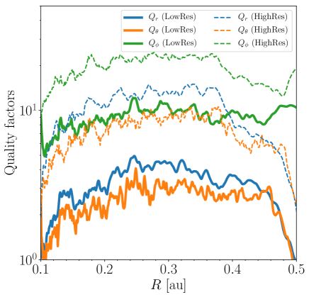
Figure 35: Radial distribution of the quality factors $Q_{r}$, $Q_{\theta}$, and $Q_{\phi}$ averaged over $0\leq\phi\leq 2\pi$ and $|z|\leq H$ at $t=300t_{\mathrm{K0}}$. The thick-solid and thin-dashed lines correspond to the results of LowRes and HighRes, respectively.

Figure 35 shows the radial profiles of $Q_{r}$, $Q_{\theta}$, and $Q_{\phi}$ averaged over $0\leq\phi\leq 2\pi$ and $|z|<H$ both for LowRes and HighRes runs. HighRes run barely satisfies the condition derived by Sorathia et al. (2012). By contrast, for LowRes run, the fastest growing mode is not resolved in our simulation although the MRI at longer wavelengths can be captured because $Q_{\phi}$ is around 10 for $r>0.2~{}$au and $Q_{\theta}$ is around 3.

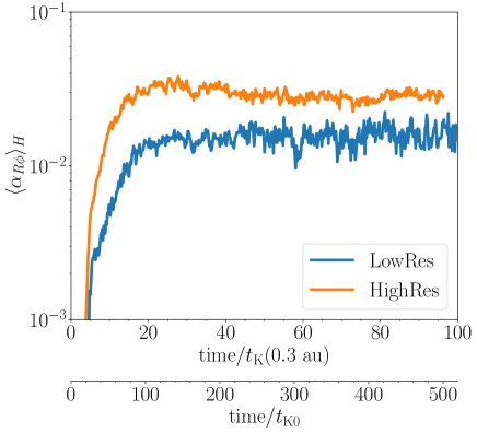
Figure 36: Time evolution of $\langle\alpha_{R\phi}\rangle_{H}$ at $R=0.3~{}\mathrm{au}$ for LowRes and HighRes.

Figure 36 compares the time evolution of $\langle\alpha_{R\phi}\rangle$ (Equation (36) between LowRes and HighRes runs. Both models show that the MRI turbulence is saturated after $t\sim 20t_{\mathrm{K}}(R=0.3~{}\mathrm{au})$. The saturation level of $\langle\alpha_{R\phi}\rangle_{H}$ is about twice larger for HighRes than for LowRes runs, consistent with the fact that LowRes run does not resolve the MRI turbulence sufficiently. The saturation level $\langle\alpha_{R\phi}\rangle_{H}\sim 2.8\times 10^{-2}$ for HighRes run is comparable to those found in local shearing-box simulations (e.g., Hawley et al., 1995; Sano et al., 2004). We confirmed that HighRes run is expected to provide converged results by measuring the so-called quality factors (Noble et al., 2010).

Appendix B MRI Turbulence in the Active Zone

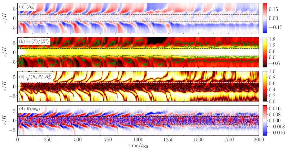
Figure 37: Spacetime diagram for (a) $\langle B_{\phi}\rangle$, (b) $8\pi\langle P\rangle/\langle B^{2}\rangle$, (c) $\sqrt{\langle B_{\phi}\rangle^{2}/\langle B_{\phi}^{2}\rangle}$, (d) $R\langle\rho v_{R}\rangle$ at $R=0.3$ au in the active zone. In Panel (b), the contours of $8\pi\langle P\rangle/\langle B^{2}\rangle$ at $R=0.3~{}\mathrm{au}$ are displayed. In each panel, the two horizontal dashed lines show the positions of $z=\pm 2H$.

Evolution of the MRI-driven turbulence is characterized by magnetic-field amplification owing to the channel flows followed by dissipation (Sano & Inutsuka, 2001). The time evolution of the vertical structures at $R=0.3~{}$au is shown in Figure 37.

Figure 37a shows that the vertical structure of $\langle B_{\phi}\rangle$ changes around $|z|\sim 2H$ (Suzuki & Inutsuka, 2009). Around the mid-plane for $|z|<2H$, the gas pressure dominates over the magnetic pressure, and the magnetic fields are amplified by the MRI dynamo activity. At $|z|\sim 2H$, the magnetic pressure becomes comparable to the gas pressure (Figure 37b), and the maximum growth scale of the MRI is comparable to $H$ since it is expressed as $2\pi v_{\mathrm{A}}/\Omega_{0}$. As a result, the magnetic fields are amplified by the channel flow whose scale is comparable to $H$, and are dissipated by magnetic reconnection. The $t$-$z$ diagram of $B_{\phi}$ shows a clear so-called butterfly structure where $B_{\phi}$ flips its sign quasi-periodically and drifts toward upper atmospheres. The timescale of the quasi-periodic activity is about a few tens rotations, which is consistent with local shearing-box simulations with stratified density structures.

Figure 37c shows $\sqrt{\langle B_{\phi}\rangle^{2}/\langle B_{\phi}^{2}\rangle_{\phi}}$ which is an indicator of the contribution of the coherent component of $B_{\phi}$ to the total toroidal field strength. The coherent field component dominates in the upper atmosphere for $|z|>2H$ while the field structure is controlled by the MRI turbulence in the disk ($|z|<2H$).

The gas motion is affected by the magnetic field structures. As shown in Figure 37d, $R\langle\rho v_{R}\rangle$ stochastically changes owing to the MRI turbulence for $|z|<2H$, it has a coherent quasi-periodic structure in the upper atmosphere. The time variability of $R\langle\rho v_{R}\rangle$ is correlated with that of $\langle B_{\phi}\rangle$. This suggests that the magnetic torque of the coherent magnetic field drifting upwards for $|z|>2H$ drives the coherent gas motion near the surface layers.

In the long term evolution, Figure 37 shows that MRI dynamo at $R=0.3~{}\mathrm{au}$ is somewhat weakened and the plasma $\beta$ starts to increase when $t\gtrsim 1300t_{\mathrm{K0}}$ corresponding to $250t_{\mathrm{K}}(R=0.3~{}\mathrm{au})$. This is related to the formation of ring structures shown in Section 3.2.1.

References

- Armitage (1998) Armitage, P. J. 1998, ApJ, 501, L189
- Bai (2013) Bai X.-N. 2013, ApJ, 772, 96
- Bai (2017) Bai X.-N. 2017, ApJ, 845, 75
- Bai & Goodman (2009) Bai X.-N. & Goodman J. 2009, ApJ, 701, 737
- Bai & Stone (2011) Bai X.-N. & Stone J. M. 2011, ApJ, 736, 144
- Bai & Stone (2013) Bai X.-N. & Stone J. M. 2013, ApJ, 769, 76
- Bai & Stone (2014) Bai X.-N. & Stone J. M. 2014, ApJ, 796, 31
- Bai & Stone (2017) Bai X.-N. & Stone J. M. 2017, ApJ, 836, 46
- Bai et al. (2016) Bai X.-N., Ye J., Goodman J., & Yuan F. 2016, ApJ, 818, 152
- Balbus & Hawley (1991) Balbus, S. A., & Hawley, J. F. 1991, ApJ, 376, 214
- Beckwith et al. (2009) Beckwith K., Hawley J. F., & Krolik J. H. 2009, ApJ, 707, 428
- Béthune et al. (2017) Béthune W., Lesur G., Ferreira J., 2017, A&A, 600, A75
- Blaes & Balbus (1994) Blaes O. M., & Balbus S. A., 1994, ApJ, 421, 163
- Blandford & Payne (1982) Blandford R. D., & Payne D. G. 1982, MNRAS, 199, 883
- Blum & Wurm (2000) Blum J., & Wurm G. 2000, Icarus, 143, 138
- Brandenburg & Zweibel (1994) Brandenburg A., & Zweibel E. G. 1994, ApJ, 427, L91
- Chandrasekhar (1961) Chandrasekhar, S. 1961, Hydrodynamic and hydromagnetic stability
- Chiang & Goldreich (1997) Chiang E. I., & Goldreich P. 1997, ApJ, 490, 368
- Cui & Bai (2021) Cui C., & Bai X.-N. 2021, MNRAS, 507, 1106
- Cui & Lin (2021) Cui C., & Lin M.-K. 2021, MNRAS, 505, 2983
- Desch & Turner (2015) Desch S. J., & Turner N. J. 2015, ApJ, 811, 156
- Dzyurkevich et al. (2010) Dzyurkevich N., Flock M., Turner N. J., Klahr H., & Henning T., 2010, A&A, 515, A70
- Evans & Hawley (1988) Evans C. R., & Hawley J. F. 1988, ApJ, 332, 659
- Fleming & Stone (2003) Fleming T., & Stone J. M. 2003, ApJ, 585, 908
- Flock et al. (2017) Flock M., Fromang S., Turner N. J., & Benisty M., 2017, ApJ, 835, 230
- Gammie (1996) Gammie C. F. 1996, ApJ, 457, 355
- Gardiner et al. (2008) Gardiner T. A., & Stone J. M. 2008, Journal of Computational Physics, 227, 4123
- Gressel et al. (2015) Gressel O., Turner N. J., Nelson R. P., & McNally C. P. 2015, ApJ, 801, 84
- Gressel et al. (2020) Gressel O., Ramsey J. P., Brinch C., Nelson R. P., Turner N. J., & Bruderer S. 2020, ApJ, 896, 126
- Guilet & Ogilvie (2012) Guilet J., & Ogilvie G. I. 2012, MNRAS, 424, 2097
- Hawley (2001) Hawley J. F. 2001, ApJ, 554, 534
- Hawley et al. (1995) Hawley J. F., Gammie C. F., & Balbus S. A., 1995, ApJ, 440, 742
- Hawley et al. (2011) Hawley J. F., Guan X., & Krolik J. H. 2011, ApJ, 738, 84
- Hawley et al. (2013) Hawley J. F., Richers S. A., Guan X., & Krolik J. H., 2013, ApJ, 772, 102
- Hirose & Turner (2011) Hirose S., & Turner N. J. 2011, ApJ, 732, L30
- Igea & Glassgold (1999) Igea J., & Glassgold A. E. 1999, ApJ, 518, 848
- Jacquemin-Ide et al. (2021) Jacquemin-Ide J., Lesur G., & Ferreira J. 2021, A&A, 647, A192
- Jin (1996) Jin L. 1996, ApJ, 457, 798
- Kretke et al. (2009) Kretke K. A., Lin D. N. C., Garaud P., & Turner N. J. 2009, ApJ, 690, 407
- Kunz (2008) Kunz M. W. 2008, MNRAS, 385, 1494
- Kunz & Balbus (2004) Kunz M. W., & Balbus S. A. 2004, MNRAS, 348, 355
- Latter & Kunz (2022) Latter H. N., & Kunz M. W. 2022, MNRAS, 511, 1182
- Latter & Papaloizou (2018) Latter H. N., & Papaloizou J. 2018, MNRAS, 474, 3110
- Lesur (2021) Lesur G. R. J. 2021, A&A, 650, A35
- Lightman & Eardley (1974) Lightman A. P., & Eardley D. M. 1974, ApJ, 187, L1
- Lovelace et al. (1999) Lovelace R. V. E., Li H., Colgate S. A., & Nelson A. F. 1999, ApJ, 513, 805
- Lubow et al. (1994) Lubow S. H., Papaloizou J. C. B., & Pringle J. E. 1994, MNRAS, 267, 235
- Lynden-Bell & Pringle (1974) Lynden-Bell D., & Pringle J. E. 1974, MNRAS, 168, 603
- Lyra & Mac Low (2012) Lyra W., & Mac Low M.-M. 2012, ApJ, 756, 62
- Meyers et al. (2014) Meyer C. D., Balsara D. S., & Aslam T. D. 2014, Journal of Computational Physics, 257, 594
- Miyoshi & Kusano (2005) Miyoshi T., & Kusano K. 2005, Journal of Computational Physics, 208, 315
- Montesinos et al. (2009) Montesinos B., Eiroa C., Mora A., Merín B., 2009, A&A, 495, 901
- Mori et al. (2019) Mori S., Bai X.-N., & Okuzumi S. 2019, ApJ, 872, 98
- Nakano et al. (2002) Nakano T., Nishi R., & Umebayashi T. 2002, ApJ, 573, 199
- Nelson et al. (2013) Nelson R. P., Gressel O., & Umurhan O. M. 2013, MNRAS, 435, 2610
- Noble et al. (2010) Noble S. C., Krolik J. H., & Hawley J. F. 2010, ApJ, 711, 959
- Okuzumi (2009) Okuzumi S. 2009, ApJ, 698, 1122
- Okuzumi & Hirose (2011) Okuzumi S., & Hirose S., 2011, ApJ, 742, 65
- Ono et al. (2016) Ono T., Muto T., Takeuchi T., & Nomura H. 2016, ApJ, 823, 84
- Ono et al. (2018) Ono T., Muto T., Tomida K., & Zhu Z. 2018, ApJ, 864, 70
- Perez-Becker & Chiang (2011) Perez-Becker D., & Chiang E. 2011, ApJ, 735, 8
- Pinilla et al. (2016) Pinilla P., Flock M., Ovelar M. d. J., & Birnstiel T. 2016, A&A, 596, A81
- Pucci et al. (2021) Pucci F., Tomida K., Stone J., Takasao S., Ji H., & Okamura S. 2021, ApJ, 907, 13
- Riols & Lesur (2018) Riols A., & Lesur G. 2018, A&A, 617, A117
- Riols & Lesur (2019) Riols A., & Lesur G., 2019, A&A, 625, A108
- Salmeron & Wardle (2003) Salmeron R., & Wardle M. 2003, MNRAS, 345, 992
- Salvesen et al. (2016) Salvesen G., Simon J. B., Armitage P. J., & Begelman M. C. 2016, MNRAS, 457, 857
- Sano & Inutsuka (2001) Sano T., & Inutsuka S. 2001, ApJ, 561, L179
- Sano & Miyama (1999) Sano T., & Miyama S. M. 1999, ApJ, 515, 776
- Sano et al. (2004) Sano T., Inutsuka S., Turner N. J., & Stone J. M. 2004, ApJ, 605, 321
- Scepi et al. (2018) Scepi N., Lesur G., Dubus G., & Flock M. 2018, A&A, 620, A49
- Shakura & Sunyaev (1973) Shakura N. I., & Sunyaev R. A. 1973, A&A, 24, 337
- Sorathia et al. (2012) Sorathia K. A., Reynolds C. S., Stone J. M., & Beckwith K. 2012, ApJ, 749, 189
- Steinacker & Papaloizou (2002) Steinacker A., & Papaloizou J. C. B. 2002, ApJ, 571, 413
- Stone et al. (2008) Stone J. M., Gardiner T. A., Teuben P., Hawley J. F., & Simon J. B. 2008, ApJS, 178, 137
- Stone et al. (2020) Stone J. M., Tomida K., White C. J., & Felker K. G. 2020, ApJS, 249, 4
- Suriano et al. (2018) Suriano S. S., Li Z.-Y., Krasnopolsky R., & Shang H. 2018, MNRAS, 477, 1239
- Suriano et al. (2019) Suriano S. S., Li Z.-Y., Krasnopolsky R., Suzuki T. K., & Shang H. 2019, MNRAS, 484, 107
- Suzuki (2023) Suzuki, T. K. 2023, PASJ, 957, 99
- Suzuki & Inutsuka (2009) Suzuki T. K., & Inutsuka S. 2009, ApJ, 691, L49
- Suzuki & Inutsuka (2014) Suzuki T. K., & Inutsuka S. 2014, ApJ, 784, 121
- Suzuki et al. (2010) Suzuki T. K., Muto T., & Inutsuka S. 2010, ApJ, 718, 1289
- Takasao et al. (2018) Takasao S., Tomida K., Iwasaki K., & Suzuki T. K. 2018, ApJ, 857, 4
- Takasao et al. (2019) Takasao S., Tomida K., Iwasaki K., & Suzuki T. K. 2019, ApJ, 878, L10
- Turner & Sano (2008) Turner N. J., & Sano T. 2008, ApJ, 679, L131
- Ueda et al. (2019) Ueda T., Flock M., & Okuzumi S. 2019, ApJ, 871, 10
- Umebayashi & Nakano (1981) Umebayashi T., & Nakano T. 1981, PASJ, 33, 617
- Velikhov (1959) Velikhov, E. P. 1959, Sov. Phys. J. Exp. Theor. Phys., 36, 1959
- Wada et al. (2013) Wada K., Tanaka H., Okuzumi S., Kobayashi H., Suyama T., Kimura H., Yamamoto T. 2013, A&A, 559, A62
- Wardle et al. (1999) Wardle M. 1999, MNRAS, 307, 849
- Xu & Bai (2016) Xu R., & Bai X.-N., 2016 ApJ, 819, 68
- Zanni et al. (2007) Zanni C., Ferrari A., Rosner R., Bodo G., & Massaglia S. 2007, A&A, 469, 811
- Zhu & Stone (2018) Zhu Z., & Stone J. M. 2018, ApJ, 857, 34
- Ferreira (1997) Ferreira J. 1997, A&A, 319, 340.
- Pelletier & Pudritz (1992) Pelletier G. & Pudritz R. E. 1992, ApJ, 394, 117
- Finocchi & Gail (1997) Finocchi, F. & Gail, H.-P. 1997, A&A, 327, 825
- van der Marel (2023) van der Marel, N 2023, Eur. Phys. J. Plus, 138, 225