Risk-averse decision strategies for influence diagrams using rooted junction trees

Abstract

This paper focuses on a mixed-integer programming formulation for influence diagrams, based on a gradual rooted junction tree representation of the diagram. We show that different risk considerations, including chance constraints and conditional value-at-risk, can be incorporated into the formulation with targeted, appropriate modifications to the diagram structure. The computational performance of the formulation is assessed on two example problems and is found to be highly dependent on the structure of the junction tree.

[label1]organization=Department of Mathematics and Systems Analysis,addressline=Aalto University, School of Science, postcode=FI-00076 Aalto, country=Finland

1 Introduction

Influence diagrams (ID) [11] are an intuitive structural representation of decision problems with uncertainties and interdependencies between random events, decisions and consequences. Traditional solution methods for influence diagrams [25] often require strong assumptions such as the no-forgetting assumption. Lauritzen and Nilsson [16] present the notion of limited memory influence diagrams (LIMID) that, albeit more general in terms of representation capabilities, do not satisfy the no-forgetting assumption and, therefore, are not amenable to these traditional methods.

The algorithms presented in the literature for solving decision problems represented as IDs are mostly suited only to problems where an expected utility function is maximized and no additional constraints are considered. Thus, often risk considerations are encoded in the utility function itself, by making it concave using, e.g., utility extraction techniques [4, 20, 8].

Very often, utility functions represent monetary values, such as costs or revenues. In that case, maximizing expected utility assumes a risk-neutral stance from the decision-maker. However, decision-makers may still have different risk tolerance profiles, which must be represented in the decision process.

There are numerous ways to incorporate risk aversion into decision models without requiring utility extraction techniques. A typical method is to minimize a risk measure instead of expected utility [18]. A commonly used measure is the Conditional Value-at-Risk (CVaR), which measures the expected loss value in the $\alpha$-tail, $\alpha$ being a confidence level parameter [22]. Another typical way of incorporating risk aversion is to use constraints such as those related to chance events or budget violations [2]. Both mentioned methods have been used widely in various applications (See, e.g., [6, 27, 13]). The main challenge with all of these is that they connect different decisions so that methods based on local computations (e.g., decision trees) cannot be straightforwardly employed.

Recently, two different mixed-integer programming (MIP) reformulations for influence diagrams have emerged, likely stemming from the considerable computational improvements in MIP solution methods. The reformulation considered in this paper is originally presented in Parmentier et al. [21], where the authors first show how to convert a LIMID representing an expected utility maximization problem into a gradual rooted junction tree. This junction tree consists of clusters of nodes from the LIMID and is reformulated as a MIP problem using marginal probability distributions of nodes within each cluster.

In contrast, Salo et al. [23] present decision programming, which directly reformulates a LIMID as a mixed-integer linear programming (MILP) formulation without the intermediate clustering step of forming a junction tree. The main advantage of decision programming is that its formulation can be adapted to minimize (conditional) value-at-risk, and its path-based MILP formulation makes it easy to consider different constraints, as discussed in Hankimaa et al. [10].

Comparing the two approaches, the clustering step employed in Parmentier et al. [21] generally results in considerably improved computational performance compared to decision programming. Against this backdrop, this paper presents an approach to incorporate the risk measures and constraints from Salo et al. [23] and Hankimaa et al. [10] in the rooted junction tree reformulation proposed by Parmentier et al. [21]. This allows us to enjoy the modelling flexibility of Decision Programming while reaping the computational benefits of the junction tree reformulation.

In Section 2, we present background on (limited memory) influence diagrams and the MIP reformulations of such diagrams. Section 3 continues with extending the rooted junction tree-based reformulation to consider different risk measures and constraints, demonstrated in two example problems in Section 4. Finally, Section 5 concludes the paper with ideas on future research directions and the potential of reformulating influence diagrams as MIP problems.

2 Background

2.1 Pig farm problem

The pig farm problem is an example of a partially observable Markov decision process (POMDP) and is used throughout this paper as the running example to illustrate the proposed developments. Cohen and Parmentier [3] further discuss the modelling of POMDPs using the methodology from Parmentier et al. [21], but we keep our focus on the more general formulations presented in the latter.

In the pig farm problem [16], a farmer is raising pigs for a period of four months after which the pigs will be sold. During the breeding period, a pig may develop a disease, which negatively affects the retail price of the pig at the time they are sold. In the original formulation, a healthy pig commands a price of 1000 DKK and an ill pig commands a price of 300 DKK. During the first three months, a veterinarian visits the farm and tests the pigs for the disease. The specificity (or true negative rate) of the test is 80%, whereas the sensitivity (true positive rate) is 90%. Based on the test results, the farmer may decide to inject a medicine, which costs 100 DKK. The medicine cures an ill pig with a probability of 0.5, whereas an ill pig that is not treated is spontaneously cured with a probability of 0.1. If the medicine is given to a healthy pig, the probability of developing the disease in the subsequent month is 0.1, whereas the probability without the injection is 0.2. In the first month, a pig has the disease with a probability of 0.1.

2.2 Influence Diagrams

An influence diagram is a directed acyclic graph $G=(N,A)$, where $N$ is the set of nodes and $A$ is the set of arcs. Let $N=N^{C}\cup N^{D}\cup N^{V}$ be the set of chance nodes $N^{C}$, value nodes $N^{V}$ and decision nodes $N^{D}$ in the influence diagram. Let $I(j),j\in N$, denote the information set (also often called parents) of $j$, i.e., nodes from which there is an arc to $j$. The influence diagram of the pig farm problem is presented in Figure 1.

Each node $j\in N$ has a discrete and finite state space $S_{j}$ representing possible outcomes. The outcome (i.e., state) $s_{j}$ of a stochastic node $m\in N^{C}\cup N^{V}$ is a random variable with a probability distribution $\mathbb{P}(X_{m}=s_{m}\mid X_{I(m)}=s_{I(m)})$, where the notation $X_{j}=s_{j}$ means that the node(s) $j$ attain the state(s) $s_{j}$. The states of a value node $v\in N^{V}$ represent different outcomes that have a utility value $u(s_{v})$ associated with them. The outcome of a decision node $d\in N^{D}$ is determined by a decision strategy $\delta(s_{d}\mid s_{I(d)}):S_{I(d)}\cup S_{d}\to\{0,1\}$.

The solution of an influence diagram is a decision strategy that optimizes the desired metric, typically expected utility, at value nodes. A common additional assumption is perfect recall, meaning that previous decisions can be recalled in later stages. Under this assumption, the optimal decision strategy may be obtained by arc reversals and node removals [24] or dynamic programming [26], for example.

Perfect recall is a rather strict assumption and in many applications, it does not hold. This challenge is circumvented with limited memory influence diagrams [16]. Many algorithms for solving the decision strategy that maximizes the expected utility have been developed, such as the single policy update [16], multiple policy updating [17], branch and bound search [12] and the aforementioned methods converting the influence diagram to a MI(L)P [21, 23].

2.3 Rooted Junction Trees

An influence diagram $G=(N,A)$ can be represented as a directed rooted tree $\mathscr{G}=(\mathscr{V},\mathscr{A})$ composed of clusters $C\in\mathscr{V}$, which are subsets of the nodes of the ID, that is, $C\subset N$. Both $G$ and $\mathscr{G}$ are directed acyclic graphs whose vertices are connected with directed arcs in $A$ and $\mathscr{A}$, respectively. The main difference between these diagrams lies in the nature of the vertices. In an influence diagram, the set of nodes $N$ consists of individual chance events, decisions and consequences, while the clusters in $\mathscr{V}$ comprise multiple nodes, hence the notational distinction between $N$ and $\mathscr{V}$.

In order to reformulate this tree into a MIP model, we impose additional conditions, making $\mathscr{G}$ a gradual rooted junction tree. Definition 2.1 states the necessary properties of a gradual rooted junction tree.

Definition 2.1.

A directed rooted tree $\mathscr{G}=(\mathscr{V},\mathscr{A})$ consisting of clusters $C\in\mathscr{V}$ of nodes $j\in N$ is a gradual rooted junction tree corresponding to the influence diagram $G$ if

1. given two clusters $C_{1}$ and $C_{2}$ in the junction tree, any cluster $C$ on the unique undirected path between $C_{1}$ and $C_{2}$ satisfies $C_{1}\cap C_{2}\subset C$;

2. each cluster $C\in\mathscr{V}$ is the root cluster of exactly one node $j\in N$ (that is, the root of the subgraph induced by the clusters with node $j$) and all nodes $j\in N$ appear in at least one of the clusters;

3. and, for each cluster, $I(j)\in C_{j}$, where $C_{j}$ is the root cluster of $j\in N$.

A rooted tree satisfying part (a) in Definition 2.1 is said to satisfy the running intersection property. This condition is sufficient for making $\mathscr{G}$ a rooted junction tree (RJT). In addition, as a consequence of part (b), we see that a gradual RJT has as many clusters as the original influence diagram has nodes, and each node $j\in N$ can be thought as corresponding to one of the clusters $C\in\mathscr{V}$. Because of this, we refer to clusters using the corresponding nodes $j\in N$ in the influence diagram as the root cluster of node $j\in N$, which is denoted as $C_{j}\in\mathscr{V}$.

Formulating an optimization model based on the gradual RJT representation starts by introducing a vector of moments $\mu_{C_{j}}$ for each cluster $C_{j},\ j\in N$. Parmentier et al. [21] show that for RJTs, we can impose constraints so that these become moments of a distribution $\mu_{N}$ that factorizes according to $G(N,A)$. The joint distribution $\mathbb{P}$ is said to factorize [14] according to $G$ if $\mathbb{P}$ can be expressed as

$$\mathbb{P}(X_{N}=s_{N})=\prod_{j\in N}\mathbb{P}(X_{j}=s_{j}\mid X_{I(j)}=s_{I(j)}).$$ (1)

In the formulation, $\mu_{C_{j}}(s_{C_{j}})$ represents the probability of the nodes within the cluster $C_{j}$ being in states $s_{C_{j}}$ and part (c) of Definition 2.1 ensures that $\mathbb{P}(X_{j}=s_{j}\mid X_{I(j)}=s_{I(j)})$ can thus be obtained from $\mu_{C_{j}}(s_{C_{j}})$ for each $j\in N$. The resulting MIP model is

$$\max \sum_{j\in N^{V}}\sum_{s_{C_{j}}\in S_{C_{j}}}\mu_{C_{j}}(s_{C_{j}})u_{C_{j}}(s_{C_{j}})$$ (2)

s.t. $$\sum_{s_{C_{j}}\in S_{C_{j}}}\mu_{C_{j}}(s_{C_{j}})=1,\ \forall j\in N$$ (3)

$$\sum_{\begin{subarray}{c}s_{C_{i}}\in S_{C_{i}},\\ s_{C_{i}\cap C_{j}}=s^{*}_{C_{i}\cap C_{j}}\end{subarray}}\mu_{C_{i}}(s_{C_{i}})=\sum_{\begin{subarray}{c}s_{C_{j}}\in S_{C_{j}},\\ s_{C_{i}\cap C_{j}}=s^{*}_{C_{i}\cap C_{j}}\end{subarray}}\mu_{C_{j}}(s_{C_{j}}),$$

$$\qquad\qquad\qquad\qquad\ \forall(C_{i},C_{j})\in\mathscr{A},s^{*}_{C_{i}\cap C_{j}}\in S_{C_{i}\cap C_{j}}$$ (4)

$$\mu_{C_{j}}(s_{C_{j}})=\mu_{\overline{C}_{j}}(s_{\overline{C}_{j}})p(s_{j}\mid s_{I(j)}),\ \forall j\in N^{C}\cup N^{V},s_{C_{j}}\in S_{C_{j}}$$ (5)

$$\mu_{C_{j}}(s_{C_{j}})=\mu_{\overline{C}_{j}}(s_{\overline{C}_{j}})\delta(s_{j}\mid s_{I(j)}),\ \forall j\in N^{D},s_{C_{j}}\in S_{C_{j}}$$ (6)

$$\mu_{C_{j}}(s_{C_{j}})\geq 0,\ \forall j\in N,s_{C_{j}}\in S_{C_{j}}$$ (7)

$$\delta(s_{j}\mid s_{I(j)})\in\{0,1\},\ \forall j\in N^{D},s_{j}\in S_{j},s_{I(j)}\in S_{I(j)}.$$ (8)

The formulation (2)-(8) is an expected utility maximization problem where $u_{C_{j}}$ in the objective function (2) represents the utility values associated with different realizations of the nodes within the cluster $C_{j}$, and $\overline{C}_{j}=C_{j}\setminus j$ is used in constraints (5) and (6) for notational brevity. Constraints (3) and (7) state that the variables $\mu_{C_{j}}$ must represent valid probability distributions, with nonnegative probabilities summing to one.

Constraint (4) enforces local consistency between adjacent clusters, meaning that for a pair $C_{i},C_{j}$ of adjacent clusters, the marginal distribution for the nodes in both $C_{i}$ and $C_{j}$ (that is, $C_{i}\cap C_{j}$) must be the same when obtained from either $C_{i}$ or $C_{j}$.

To ease the notation, moments $\mu_{\overline{C}_{j}}(s_{\overline{C}_{j}})=\sum_{s_{j}\in S_{j}}\mu_{C_{j}}(s_{C_{j}})$ are used in constraints (5) and (6). The expression $\mu_{\overline{C}_{j}}$ represents the marginal distribution for cluster $C_{j}$ with the node $j$ marginalized out. The value $p(s_{j}\mid s_{I(j)})$ is the conditional probability of a state $s_{j}$ given the information state $s_{I(j)}$ and $\delta(s_{j}\mid s_{I(j)})$ the decision strategy in node $j\in N^{D}$. It should be noted that constraint (6) involves a product of two variables, and is thus not linear. Since we are limiting ourselves to settings with deterministic strategies (i.e., $\delta(s_{d}\mid s_{I(d)}):S_{I(d)}\cup S_{d}\to\{0,1\}$), these constraints become indicator constraints and can be efficiently handled by solvers such as Gurobi [9]. We remark that this would not be the case for more general strategies of the form $\delta(s_{d}\mid s_{I(d)}):S_{I(d)}\cup S_{d}\to[0,1]$.

Any rooted tree satisfying the properties in Definition 2.1 is a gradual RJT and can therefore be used to obtain a valid version of model (2)-(8). For instance, a junction tree where each cluster $C_{j}$, $j\in N$, contains the nodes $i\in N$ such that $i\leq j$ would satisfy the definition. However, this would result in large clusters, and consequently, a large number of constraints (4)-(6). It is thus important to find a gradual RJT representation where the clusters are as small as possible. Parmentier et al. [21] present two algorithms for creating a gradual RJT from an ID. The first algorithm uses a given topological order of the nodes and builds the RJT starting from the last cluster and proceeding in the reverse direction of this topological order. This algorithm returns a gradual RJT with minimal clusters given the ordering of nodes. The second algorithm has an additional step of finding a “good” topological order that would lead to smaller clusters. The contribution of this paper is focused on modifying the underlying influence diagram to which both algorithms can be applied. For simplicity, we chose to use the algorithm requiring a topological order in the examples of this paper. Using $H_{1},T_{1},D_{1},V_{1},H_{2},...,H_{4},V_{4}$ as a topological order, the pig farm influence diagram in Figure 1 is transformed to the gradual RJT in Figure 2.

Figure 1: The pig farm problem [16].

Figure 2: Gradual RJT of the pig farm problem.

3 Our contributions

3.1 Extracting the utility distribution

For problems with multiple value nodes, e.g., multi-stage decision problems, the expected utility has the convenient property that the total expected utility is the sum of expected utilities in each value node. This property can be exploited in the solution process, and for this reason, many solution methods for influence diagrams, including the RJT approach in Parmentier et al. [21], only tackle maximum expected utility (MEU) problems.

In contrast, risk measures (such as CVaR) require that the full probability distribution of the consequences is explicitly represented in the model. However, such representations are lost when the value nodes are placed in separate clusters, as in Figure 2, since the probability distributions are only defined for each cluster separately. For example, in the pig farm problem described in Section 2.1, the joint distribution of $V_{1}$ and $V_{2}$ cannot be inferred from the probability distributions of clusters $C_{V_{1}}$ and $C_{V_{2}}$, as we cannot assume the probabilities of consequences in $V_{1}$ and $V_{2}$ to be independent.

We note that after solving the model (2)-(8), any distribution can be obtained for the MEU solution. As stated in Definition 2.1, part (c), the rooted junction trees in this paper have $I(j)\subseteq C_{j}$ by construction, and we can thus use the optimal values $\bar{\mu}_{j}$ to obtain $\mathbb{P}(X_{j}=s_{j}\mid X_{I(j)}=s_{I(j)})$ for all nodes $j\in N$, and consequently use Eq. 1 to obtain $\overline{\mu}_{N}$. Then, we can obtain the marginal distribution for nodes $N_{1}\subset N$ by marginalizing out $N\setminus N_{1}$. More formally,

$$\mathbb{P}(s^{*}_{N_{1}})=\sum_{s_{N}\in\{S_{N}\mid s_{N_{1}}=s^{*}_{N_{1}}\}}\overline{\mu}_{N}.$$

Using this approach for incorporating constraints and objectives involving the utility distribution of multiple value nodes in (2)-(8) would require obtaining the distribution $\mu_{N}$ within the model. This, however, would require products of arbitrarily many continuous variables $\mu_{C_{j}}$ within the model, resulting in nonlinearity and the associated computational challenges.

The issue can be circumvented by modifying the influence diagram such that the consequences of the problem are represented by a single value node. Generally, multiple value nodes represent components of a separable utility function such that $U(s)=\sum_{v\in N^{V}}U_{v}(s_{I(v)})$ [26] and, being such, the value nodes can be combined under a single value node $\bar{v}$, in which the consequences can simply be evaluated with $U(s_{I(\bar{v})})$.

This transformation requires that arcs $(p,\bar{v}),\forall v\in N^{V},p\in I(v)$, are added to $A$. Then, according to Definition 2.1, part (c), we have that $\cup_{v\in V}I(v)\subset C_{\bar{v}}$. Consequently, the marginal probability distribution $\mu_{C_{\bar{v}}}$ contains information on the joint probability $\mathbb{P}(\cap_{v\in N^{v}}v)$ and this can be exposed to produce a probability distribution for utility values. Following this approach, the modified influence diagram of the modified pig farm problem is presented in Figure 3 and the corresponding gradual RJT in Figure 4.

This however, incurs in computationally more demanding versions of model (2)-(8). In the modified pig farm problem, all nodes $D_{k}$ are in the information set of $\bar{V}$, and it follows from the running intersection property that $D_{k}$ must be contained in every cluster that is in the undirected path between $C_{D_{k}}$ and $C_{\bar{v}}$. Therefore, the clusters become larger as the parents of value nodes are “carried over”, instead of evaluating separable components of the utility function at different value nodes. As will be discussed in Section 3.4, this transformation comes with a cost on the computational efficiency.

Figure 3: The pig farm problem reformulated [16].

Figure 4: Gradual RJT of the reformulated pig farm problem.

3.2 Imposing chance, logical, and budget constraints

The proposed reconfiguration of the influence diagram allows us to expose the vector of moments of the value node $\bar{v}$, which in turn, enables the formulation of a broad range of risk-aversion-related constraints.

For example, a chance constraint can be constructed based on the utility distribution from the vector of moments of the value node $\bar{v}$ as:

$$\sum_{s_{C_{\bar{v}}}\in\{S_{C_{\bar{v}}}\mid s_{{\bar{v}}}\in S^{o}_{{\bar{v}}}\}}\mu(s_{C_{\overline{v}}})\leq p,$$ (9)

where $S^{o}_{{\bar{v}}}$ is the set of outcomes that the decision maker wishes to constrain and $p\in[0,1]$. For instance, assume that a decision maker wishes to add chance constraints enforcing that the probability of the payout of the process being less than some fixed limit $l$ is at most $p$. Then $S^{o}_{\bar{v}}$ would contain all states $s_{\bar{v}}$ such that $U(s_{\bar{v}})<l$.

Chance constraints on the probability distribution of a single node can be straightforwardly added to any cluster containing the node. For instance, chance constraints enforcing that a node $n$ must be in state $s^{*}_{n}$ with a probability greater or equal than $p$ can be formulated as

$$\sum_{s_{C_{n}}\in\{S_{C_{n}}\mid s_{n}=s^{*}_{n}\}}\mu_{C}(s_{C_{n}})\geq p.$$

Note that this formulation can be enforced for any clusters $C_{k}$ such that $n\in C_{k}$. Then, to keep the number of variables in the constraint to a minimum, one can choose the smallest of such clusters, i.e., choose cluster $k^{\prime}=\arg\min_{k\in N}\{|C_{k}|,~{}n\in C_{k}\}$.

Logical constraints can be seen as a special case of chance constraints. For example, in the pig farm problem (in Section 2), the farmer may wish to attain an optimal decision strategy while ensuring that the number of injections is at most two per pig due to a limited availability of injections. Then, $S^{o}_{\bar{v}}$ would contain all realizations of the nodes in $C_{\bar{v}}$ that would lead to a violation of the constraint, i.e., the state combinations in which three injections would be given to a pig. Then, constraint (10) that makes these scenarios impossible could be imposed, i.e.,

$$\sum_{s_{C_{\bar{v}}}\in\{S_{C_{\bar{v}}}\mid s_{{\bar{v}}}\in S^{o}_{{\bar{v}}}\}}\mu(s_{C_{\overline{v}}})\leq 0.$$ (10)

Budget constraints are analogous to logical constraints, as the farmer could instead have an injection budget, say 200 DKK per pig. Then, $S^{o}_{\bar{v}}$ should contain all states $s_{\bar{v}}$, where more than 200 DKK is used for treating a pig, with the constraint enforced similarly as in (10).

3.3 Conditional Value-at-Risk

In addition to a number of utility distribution-related constraints, a single value node also enables the consideration of alternative risk measures. Next, we focus our presentation on how to maximize conditional value-at-risk. However, we highlight that other risk metrics such as absolute or lower semi-absolute deviation [23] can, in principle, be used. The entropic risk measure [7] can also be used as a constraint. However, incorporating it in the objective function is likely to introduce nonlinearity in the model due to the logarithmic nature of the measure.

The proposed formulation for conditional value-at-risk maximization is analogous to the method developed for decision programming in [23]. Denote the possible utility values with $u\in U$ and suppose we can define the probability $p(u)$ of attaining a given utility value. In the presence of a single value node, we would define $p(u)=\sum_{s_{C_{v}}\in\{S_{C_{v}}|U(s_{C_{v}})=u\}}\mu(s_{C_{v}})$. We can then pose the constraints

$$\eta-u \leq M\lambda(u),\ \forall u\in U$$ (11)

$$\eta-u \geq(M+\epsilon)\lambda(u)-M,\ \forall u\in U$$ (12)

$$\eta-u \leq(M+\epsilon)\overline{\lambda}(u)-\epsilon,\ \forall u\in U$$ (13)

$$\eta-u \geq M(\overline{\lambda}(u)-1),\ \forall u\in U$$ (14)

$$\overline{\rho}(u) \leq\overline{\lambda}(u),\ \forall u\in U$$ (15)

$$p(u)-(1-\lambda(u)) \leq\rho(u)\leq\lambda(u),\ \forall u\in U$$ (16)

$$\rho(u) \leq\overline{\rho}(u)\leq p(u),\ \forall u\in U$$ (17)

$$\sum_{u\in U}\overline{\rho}(u) =\alpha$$ (18)

$$\lambda(u),\overline{\lambda}(u) \in\{0,1\},\ \forall u\in U$$ (19)

$$\rho(u),\overline{\rho}(u) \in[0,1],\ \forall u\in U,$$ (20)

$$\eta\in\mathbb{R}$$ (21)

where $\alpha$ is the probability level in VaR_α. The constraints force the values of the decision variables to the values in Table 1.

variable	value
$\eta$	VaRα
$\lambda(u)$	1 if $u<\eta$
$\overline{\lambda}(u)$	0 if $u>\eta$
$\rho(u)$	0 if $\lambda(u)=0$, $p(u)$ otherwise
$\overline{\rho}(u)$	$\begin{cases}p(u)&\text{ if }u<\eta,\\ \alpha-\sum_{u\in U}p(u)&\text{ if }u=\eta,\\ 0&\text{ if }u>\eta\ (\bar{\lambda}(u)=0)\end{cases}$

Table 1: Variables and the corresponding values that satisfy (11)-(20)

In constraints (11)-(20), $M$ is a large positive number and $\epsilon$ is a small positive number. The parameter $\epsilon$ is used to model strict inequalities, which generally cannot be directly used in mathematical optimization solvers. For example, $x\geq\epsilon$ is assumed to be equivalent to $x>0$. When $\lambda(u)=0$, constraints (11) and (12) become $-M\leq\eta-u\leq 0$, or $\eta\leq u$. When $\lambda(u)=0$, they instead become $\epsilon\leq\eta-u\leq M$, or $\eta>u$. Constraints (13) and (14) can be examined similarly to obtain the results in Table 1.

The correct behavior of variables $\rho(u)$ is enforced by (16) and (17). If $\lambda(u)=0$, constraint (16) forces $\rho(u)$ to zero. If $\lambda(u)=1$, $\rho(u)=p(u)$. Finally, assuming $\eta$ is equal to VaR_α, now that we have $\lambda(u)=1\longrightarrow\rho(u)=p(u)$ for all $u<\eta$, the value of $\overline{\rho}(u)$ has to be $\alpha-\sum_{u\in U}\rho(u)$ for $u=\eta$. It is easy to see that $\eta$ must be equal to VaR_α for there to be a feasible solution for the other variables. For a more rigorous proof, see Salo et al. [23, Appendix A].

By introducing the constraints above to the optimization model, $CVaR_{\alpha}$ can then be obtained as $\frac{1}{\alpha}\sum_{u\in U}\overline{\rho}(u)u$. This can be either used as in the objective function or as a part of the constraints of the problem. We also note that the described approach is very versatile in that $u$ can be selected to be, e.g., a stage-specific utility function, thus allowing us to limit risk in specific stages of a multi-stage problem. Krokhmal et al. [15] discusses the implications of stage-wise CVaR-constraints in detail.

3.4 Problem size

From Definition 2.1, we can derive a relationship between the width of the tree and the size of the corresponding model. By definition, a tree with a width $k$ has a maximum cluster $C_{n}$ containing $k+1$ nodes. In a gradual RJT, the cluster $C_{n}$ includes exactly one node $n\in N$ not contained in its parent cluster $C_{i}$. Using the running intersection property, the $k$ other nodes in $C_{n}$ must also be in $C_{i}$. If we make the very light assumption that all nodes $l\in C_{i}\cup C_{n}$ have at least two states $s_{l}$, this implies that there are $\prod_{l\in C_{i}\cup C_{n}}|S_{n}|\geq 2^{k}$ local consistency constraints (4) for the pair $(C_{i},C_{n})\in\mathscr{A}$ and the number of constraints in the model (2)-(8) is thus at least $\mathcal{O}(c^{k})$, where $k$ is the width of the gradual RJT. This is in line with Parmentier et al. [21] pointing out that the RJT-based approach is only suited for problems with moderate rooted treewidth.

The width of the tree in Figure 4 is $N+1$, where $N$ is the number of treatment periods in the pig farm problem ($N=3$ in the example), while the width of the original pig farm RJT in Figure 2 is only 2. Furthermore, we note that the rooted treewidth of a problem is defined as the size of the largest cluster minus one. In an RJT, we have $(I(n)\cup n)\subset C_{n}$ for all $n\in N$ and the treewidth is thus at least $max(|I(n)|,\ n\in N)$. For the single value node pig farm problem, $|I(\bar{V})|=N+1$ and for the original pig farm problem, $|I(H_{2})|=2$. Therefore, we conclude that there are no RJT representations for these problems with a smaller width than the ones presented in Figures 2 and 4.

These results imply that the optimization model for the original pig farm problem grows linearly with the number of stages, but both the single value node pig farm grows exponentially with the number of decisions, suggesting possible computational challenges in larger problems.

4 Computational experiments

To assess the computational performance of the model (2)-(8), we use the pig farm problem described earlier and the N-monitoring problem from Salo et al. [23]. Both problems are solved with varying numbers of decision nodes, providing insights into the growth in solution times with increasing problem sizes. The models were implemented using Julia v1.7.3 [1] and JuMP v1.5.0 [5] and solved with the Gurobi solver v10.0.0 [9].

4.1 Pig farm problem

A six-month pig farm problem (five treatment periods and a final selling period) is used to highlight the use of the developed formulations. The constraints presented in Section 3.3 are added to the optimization model so that the problem can be optimized taking into account the CVaR of the chosen solution.

This enables determining nondominated strategies based on CVaR and expected utility values using, for example, the epsilon constraint method [19]. The example in Figure 5 shows the nondominated strategies based on expected utility and CVaR with probability level $\alpha=0.05$ (orange points) and a sample of the dominated strategies (blue points).

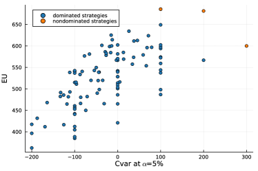
Figure 5: Nondominated strategies

The nondominated strategies from highest expected utility to lowest are:

• Treat the pig in the 4${}^{\text{th}}$ and 5${}^{\text{th}}$ period if the test result is positive

• Treat the pig in the 5${}^{\text{th}}$ period regardless of the test result

• Never treat the pig

Using the formulations presented in Section 3.2 the six-month pig farm problem can also be solved with a variety of chance constraints. For instance, we might be interested in a decision strategy that maximizes the expected utility while ensuring the following:

• A pig is healthy in the last period with a probability of 80% or higher;

• The payout is at least 800 DKK with a probability greater or equal to 50%.

The decision strategy is then to treat the pig in the 3${}^{\text{rd}}$ period if the test result is positive and in the 4${}^{\text{th}}$ and 5${}^{\text{th}}$ periods no matter the test result. This way the expected utility is 627 DKK.

4.2 N-monitoring

The N-monitoring problem [23] represents a problem of distributed decision-making where $N$ decisions are made in parallel with no communication between the decision-makers. The node $L$ in Figure 6 represents a load on a structure, nodes $R_{i}$ are reports of the load, based on which the corresponding fortification decisions $A_{i}$ are made. The probability of failure in node $F$ depends on the load and the fortification decisions, and the utility in $T$ comprises fortification costs and a reward if the structure does not fail.

Figure 6: An influence diagram representing the N-monitoring problem.

With topological order $L,R_{1},A_{1},...,R_{N},A_{N},F,T$, the rooted junction tree corresponding to the diagram in Figure 6 is presented in Figure 7. The structure of parallel observations and decisions in the N-monitoring problem is very different compared to the partially observed Markov decision process (POMDP) structure of the pig farm problem. From Figure 6, we can see that $|I(F)|=N+1$, and consequently, there are no RJT representations for the N-monitoring problem with a width less than $N+1$. In contrast, as discussed in Section 3.4, the pig farm RJT has a constant width of 2, independent of the number of decision stages. We note that the width of the RJT in Figure 7 is the same as of the single value node pig farm RJT (Figure 4). However, in the N-monitoring problem, this is a consequence of the inherent structure of the problem, instead of the influence diagram manipulation described in Section 3.1. That is, for the pig farm problem, there is a small width RJT representation for MEU problems, but such representations are impossible for the N-monitoring problem due to its structure.

Figure 7: A rooted junction tree representing the N-monitoring problem.

4.3 Computational results

Figure 8 shows the increase in solution times as the problem size increases. First, we see that the solution time for the N-monitoring problem increases the fastest. While the pig farm problem with a single value node is faster than the N-monitoring problem, the solution time seems to also increase exponentially. Finally, the solution time for the pig farm problem as presented in Section 2.1 does not change significantly. These results are in line with the analysis of model sizes in Section 3.4 and highlight the importance of keeping the cluster sizes small in junction trees. Both versions of the pig farm problem compared in Figure 8 solve exactly the same problem, but the structure of the diagram in the single value node problem increases the width of the tree, and subsequently, the model size and solution time.

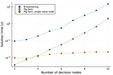
Figure 8: Mean solution times for 50 random instances in the pig farm and N-monitoring problems with 2-10 decision nodes.

Finally, we compare these results to the corresponding results using decision programming, presented in Hankimaa et al. [10]. In the N-monitoring problem and the single value node pig farm problem, we see similar exponential growth for both models, with the solution times in this paper being 2-3 orders of magnitude smaller. For the original pig farm problem, the decision programming formulation remains the same, as the model size is determined by the chance and decision nodes in the diagram. However, for this version of the problem, the solution times for (2)-(8) hardly even change with the model sizes tested in this section, illustrating the superior computational efficiency of the model with small treewidths.

5 Conclusions

In this paper, we have described a MIP reformulation of decision problems presented as (limited memory) influence diagrams, originally proposed in Parmentier et al. [21]. Our main contribution is to extend the modelling framework from Parmentier et al. [21] to embed it with more general modelling capabilities. We illustrate how, e.g., chance constraints and conditional value-at-risk can be incorporated into the formulation.

We also present some results on the relationship between the rooted treewidth of the RJT representation and the size of the corresponding MIP model, along with solution times from two different decision problems. The pig farm problem is a partially observed Markov decision process (POMDP) and very large instances can be solved to optimality within seconds. The N-monitoring problem, on the other hand, is an example of distributed decision-making, where $N$ decision-makers must make decisions in parallel with no communication between them. We found that, for such problems, the size of the formulation (2)-(8) grows exponentially with $N$, resulting in the solution times becoming considerably large for $N$ as small as 10.

We find that the model presented in Parmentier et al. [21] can be extended beyond pure expected utility maximization problems to incorporate most of the constraints and objective functions present in decision programming, the alternative MIP reformulation based on LIMIDs described in Salo et al. [23] and Hankimaa et al. [10]. The advantage of using the models described in this paper is that in terms of model size, decision programming models grow exponentially with respect to the number of nodes, which seems to be only the worst-case behaviour with rooted junction trees. Inspecting the formulation (2)-(8), we notice that the number of constraints is mainly affected by the local consistency constraints (4), as the number of all other constraints is linear in the number of nodes. The number of constraints for the pig farm RJT in Figure 2 is $\mathcal{O}(N)$, where $N$ is the number of decision stages. On the other hand, the same formulation for the N-monitoring RJT in Figure 7 has $\mathcal{O}(2^{N})$ constraints, exponential in the number of parallel decisions. For a worst-case example, in a diagram with arcs $(i,j)$ for each $i,j\in N,i<j$ (semicomplete digraph), the number of constraints would be exponential in the number of nodes.

In this paper, the extraction of relevant probability/utility distributions is made possible by modifying the underlying influence diagram. For future research, it might be beneficial to note that any gradual RJT (Definition 2.1) can be used to formulate the MIP model (2)-(8). Notably, it should be possible to modify the RJT so that relevant nodes are “carried over” to, e.g., the last cluster, giving us access to the joint probability distributions required for the models described in this paper.

References

- Bezanson et al. [2017] Bezanson, J., Edelman, A., Karpinski, S., Shah, V.B., 2017. Julia: A fresh approach to numerical computing. SIAM Review 59, 65–98.
- Charnes and Cooper [1959] Charnes, A., Cooper, W., 1959. Chance constrained programming. Management Science 6, 73–79.
- Cohen and Parmentier [2023] Cohen, V., Parmentier, A., 2023. Future memories are not needed for large classes of POMDPs. Operations Research Letters 51, 270–277.
- Davidson et al. [1957] Davidson, D., Suppes, P., Siegel, S., 1957. Decision making; an experimental approach. Decision making; an experimental approach., Stanford University Press. Pages: 121.
- Dunning et al. [2017] Dunning, I., Huchette, J., Lubin, M., 2017. JuMP: A Modeling Language for Mathematical Optimization. SIAM Review 59, 295–320.
- Filippi et al. [2020] Filippi, C., Guastaroba, G., Speranza, M., 2020. Conditional value-at-risk beyond finance: a survey. International Transactions in Operational Research 27, 1277–1319.
- Föllmer and Knispel [2011] Föllmer, H., Knispel, T., 2011. Entropic risk measures: Coherence vs. convexity, model ambiguity and robust large deviations. Stochastics and Dynamics 11, 333–351.
- Geissel et al. [2018] Geissel, S., Sass, J., Seifried, F.T., 2018. Optimal expected utility risk measures. Statistics & Risk Modeling 35, 73–87.
- Gurobi Optimization, LLC [2022] Gurobi Optimization, LLC, 2022. Gurobi Optimizer Reference Manual. URL: https://www.gurobi.com.
- Hankimaa et al. [2023] Hankimaa, H., Herrala, O., Oliveira, F., Tollander de Balsch, J., 2023. Decisionprogramming.jl – a framework for modelling decision problems using mathematical programming. arXiv:2307.13299.
- Howard and Matheson [2005] Howard, R.A., Matheson, J.E., 2005. Influence diagrams. Decision Analysis 2, 127–143.
- Khaled et al. [2013] Khaled, A., Hansen, E.A., Yuan, C., 2013. Solving limited-memory influence diagrams using branch-and-bound search, in: Uncertainty in Artificial Intelligence (UAI-13), AUAI Press, Arlington, Virginia, USA. pp. 331–341.
- Khassiba et al. [2020] Khassiba, A., Bastin, F., Cafieri, S., Gendron, B., Mongeaua, M., 2020. Two-stage stochastic mixed-integer programming with chance constraints for extended aircraft arrival management. Trasnportation Science 54, 897–919.
- Koller and Friedman [2009] Koller, D., Friedman, N., 2009. Probabilistic graphical models: principles and techniques. MIT press.
- Krokhmal et al. [2002] Krokhmal, P., Palmquist, J., Uryasev, S., 2002. Portfolio optimization with conditional value-at-risk objective and constraints. Journal of risk 4, 43–68.
- Lauritzen and Nilsson [2001] Lauritzen, S.L., Nilsson, D., 2001. Representing and solving decision problems with limited information. Management Science 47, 1235–1251.
- Mauà et al. [2012] Mauà, D.D., de Campos, C.P., Zaffalon, M., 2012. Solving limited memory influence diagrams. Journal of Artificial Intelligence Research 44, 97–140.
- Homem-de Mello and Pagnoncelli [2016] Homem-de Mello, T., Pagnoncelli, B.K., 2016. Risk aversion in multistage stochastic programming: A modeling and algorithmic perspective. European Journal of Operational Research 249, 188–199.
- Miettinen [1999] Miettinen, K.M., 1999. Nonlinear multiobjective optimization. Kluwer Academic Publishers.
- Nielsen and Jensen [2004] Nielsen, T.D., Jensen, F.V., 2004. Learning a decision maker’s utility function from (possibly) inconsistent behavior. Artificial Intelligence 160, 53–78.
- Parmentier et al. [2020] Parmentier, A., Cohen, V., Leclère, V., Obozinski, G., Salmon, J., 2020. Integer programming on the junction tree polytope for influence diagrams. INFORMS Journal on Optimization 2, 209–228.
- Rockafellar and Uryasev [2000] Rockafellar, R., Uryasev, S., 2000. Optimization of conditional value-at-risk. Journal of Risk 2, 21–42.
- Salo et al. [2022] Salo, A., Andelmin, J., Oliveira, F., 2022. Decision programming for mixed-integer multi-stage optimization under uncertainty. European Journal of Operational Research 299, 550–565.
- Shachter [1986] Shachter, R.D., 1986. Evaluating influence diagrams. Operations Research 34, 871–882.
- Shachter and Bhattacharjya [2010] Shachter, R.D., Bhattacharjya, D., 2010. Solving influence diagrams: Exact algorithms. Wiley encyclopedia of operations research and management science .
- Tatman and Shachter [1990] Tatman, J.A., Shachter, R.D., 1990. Dynamic programming and influence diagrams. IEEE Transactions on Systems, Man, and Cybernetics 30, 365–379.
- Xu et al. [2017] Xu, B., Boyce, S.E., Zhang, Y., Liu, Q., Guo, L., Zhong, P.A., 2017. Stochastic programming with a joint chance constraint model for reservoir refill operation considering flood risk. Journal of Water Resources Planning and Management 143.