Heavy Hexaquarks in the Flux Tube Model

Abstract

Hexaquarks are one of the currently emerging topics in both experimental and theoretical high energy physics. Hexaquarks have been examined in relation to particle physics, however, there are still some research and theoretical conjectures surrounding their relationship to dark matter. Due to some experimental discoveries, it has attracted much interest and also resulted in new theoretical models to study the properties of these states. In the present work, Regge trajectories of some hexaquark states are compared with tetraquark and pentaquark states. The study is mainly concentrated on fully heavy hexaquark states. The mass spectra of these hexaquark states have also been investigated and the results are compared with other theoretical works. Our findings agree well with those of other researchers.

Received (Day Month Year)Revised (Day Month Year)

PACS Nos.: 11.55.Jy. 12.40.Yx

1 Introduction

Since only color singlet multiquark states can exist in nature, one can also anticipate the possible existence of hexaquark states. This was initially proposed by Xuong and Dyson in 1964, which was called the dibaryon state.[1] In the course of time, another hexaquark state with the quark content $uuddss$ was proposed by Jaffe.[2] Hexaquarks comprise either six quarks ($qqqqqq$) or three quarks and three antiquarks ($qqq\bar{q}\bar{q}\bar{q}$). The six quark combination looks like two baryons bound together and can be called dibaryons. Hence dibaryons are the states with baryon number two. Though deuteron consists of six quarks $uuuddd$, it cannot be regarded as the compact hexaquark state, as the separation between the proton and neutron in the deuteron nucleus is large, of the order of $4fm$. These hexaquark states have been searched extensively in N-N scattering experiments.[3, 4] Specially WASA-at-COSY collaboration reported a series of experimental results in this regard.[5, 6, 7] The observation and confirmation of state $d^{*}(2380)$ indicated the existence of hexaquark and di-baryon states. [8, 5, 6, 7, 9] The mass and angular momentum of $d^{*}(2380)$ are $2380MeV$ and $J^{P}=3^{+}$ respectively. According to the most current update on the BESIII collaboration’s search for hexaquarks, no hexaquark state has been discovered.[10]

Several research groups have theoretically investigated the properties of fully heavy tetraquark states,[11, 12, 13, 14, 15, 16, 17] and the LHCb reported its experimental finding in 2020.[18] Inspired by this, a lot of theoretical studies have been made in the field of fully heavy pentaquark and hexaquark states. [19, 20, 21, 22] The quark-delocalization model,[23, 24] the flavor SU(3) skyrmion model, [25] the chiral SU(3) quark model,[26] the quark cluster model,[27, 28] are some of the initial theoretical works, where the six quark states are predicted. Wang estimated the masses of fully heavy hexaquark states using the QCD sum rules. In this case, vector currents of the diquark-diquark-diquark type are built to examine the vector and scalar hexaquark states.[21] Using a diffusion Monte Carlo method, Pelegrina and Gordillo have defined the characteristics of fully-heavy compact hexaquarks. In the current investigation, they solely took into account compact hexaquark objects and predicted the masses of states like $cccccc$, $cccccb$, $cccbbb$, $ccbbbb$, and $bbbbbb$.[22] Using the constituent quark model, Fang and colleagues have examined the mass spectra of fully heavy hexaquark states. Spin-spin interactions, the linear confinement potential, and the color Coulomb potential have all been taken into account. Their research demonstrated the existence of hexaquark resonances. These resonances will decay into heavy baryons.[29] The deuteron-like double charm hexaquark states are investigated using the complex scaling method. Here authors have considered the hexaquark states as molecules. The study mainly focussed on determining the properties of bound and resonance hexaquark states.[30] The spin-zero hexaquark state has been searched using the LQCD techniques.[31] The quenched lattice QCD study shows that the proton-antiproton state cannot be regarded as a spin-zero hexaquark state. Amarasinghe and others have studied the scattering of two-nucleon systems using the variational approach.[32] With interpolating operators such as dibaryon operators, hexaquark operators are studied in this approach. This study does not give a proper conclusion regarding the existence of two-nucleon bound states. The $d^{*}(2380)$ is the most speculated hexaquark in connection with the dark matter. Hexaquarks as dark matter is still only a theoretical hypothesis that hasn’t been substantiated with experimental confirmation. The main hypothesis is that hexaquarks could have been created in the early universe and accounted for the dark matter. Azizi and others have suggested a new particle termed the scalar hexaquark $uuddss$ as a potential dark matter candidate. The QCD sum rule approach is used to determine the hexaquark particle’s mass and coupling constant. Depending on the strange quark mass employed, their calculations for the hexaquark mass range from 1180 $MeV$ to 1239 $MeV$. [33] Bashkanov and Watts, suggested that Bose-Einstein condensates of the $d^{*}(2380)$ hexaquark could serve as a potential candidate for dark matter. Additionally, the paper explores potential astronomical signatures, such as cosmic ray events, that could certainly indicate the presence of $d^{*}(2380)$ condensates. [34]

The study of the behavior of elementary particles serves as the foundation for numerous scientific disciplines, and theoretical models like the flux tube model are crucial for improving our fundamental understanding of the cosmos. In the present work, Regge trajectories of various hexaquark states in the flux tube model are examined, and the findings are compared with those of prior theoretical studies.

The structure of this paper is as follows. In section 2, the flux tube model is used to generate equations for classical mass and angular momentum for various hexaquark configurations. In section 3, the results are then extensively explored. And the conclusions are drawn in accordance. This work examines the impact of string length variation on a few hexaquark states and compares the calculated masses of these states to other theoretical results. Further tetra, penta, and hexaquark Regge trajectories have been compared, and the findings are quite interesting.

2 Formulation

The flux tube model plays an important role in explaining the color confinement mechanism. The flux-tube model, in its most basic form, consists of a flux tube with quark and antiquark ends. It becomes a quantized Nambu string for light quarks and the potential model with linear confinement in the non-relativistic limit.[35] In the flux tube model, it is assumed that the massless quarks are lying at the ends of the string and are considered to revolve with speed of light. If the string is rotating about its midpoint, then the classical mass and the angular momentum of a hadron is related by the following equation:

$$J=\alpha_{0}+\alpha M^{2}$$ (1)

where $\alpha_{0}$ and $\alpha$ are constants with $\alpha$=1/(2$\pi K$). Here $K$ is the string tension. These Regge trajectories have proven to be quite successful in providing a comprehensive framework for understanding the various properties of mesons, baryons, and other exotic hadrons.[36, 37, 38, 39, 40, 41] Our previous work utilized the flux tube model to study the Regge trajectories of tetra and pentaquarks. According to our findings, the flux tube model offers a good framework for exploring the properties of multiquark systems.[42] In this present work, we have extended this formulation to investigate hexaquark systems, with the goal of further understanding the confinement and behavior of these complex particles in the flux tube. We have found some new and interesting results. In the flux tube model, for hexaquarks, there will be thirty one different configurations with different combinations of quarks as shown in Fig. 1. The Fig. 1 shows the set of configurations of hexaquarks with $n(=1,2,3)$ number of quark at one end of the string. The expression representing mass and angular momentum for all configurations in Fig. 1 can be modified to the following general form:[43, 44]

$$M_{n(mod)} =\sum\frac{Kl\mathcal{M}_{n}}{fM}\left(\int_{0}^{f}\frac{dv}{\sqrt{1-v^{2}}}+\int_{0}^{\frac{\sum m_{q_{n}}}{{\mathcal{M}_{n}}}f}\frac{dv}{\sqrt{1-v^{2}}}\right)$$ (2)

$$+\gamma_{0}\sum m_{q_{n}}+\gamma_{n}\mathcal{M}_{n}.$$

$$J_{n(mod)} =\frac{kl^{2}}{f^{2}}\cdot\left(\frac{\mathcal{M}_{n}}{M}\right)^{2}\left\{\int_{0}^{f}\frac{v^{2}dv}{\sqrt{1-v^{2}}}+\int_{0}^{\frac{\sum m_{q_{n}}}{\mathcal{M}_{n}}f}\frac{v^{2}dv}{\sqrt{1-v^{2}}}\right\}$$ (3)

$$+\frac{m_{q_{1}}fl}{M}\left\{\gamma_{0}\mathcal{M}_{n}+\gamma_{n}\sum m_{q_{n}}\right\}.$$

Here, $M=\sum_{i=1}^{6}m_{q_{i}}$, $\mathcal{M}_{n}$ = $M$ - $\sum m_{q_{n}}$, $\sum m_{q_{n}}=\sum_{n=1}^{n}m_{q_{n}}$where n is the number of quarks at one side of string. Whereas, $\gamma_{0}=\frac{1}{\sqrt{1-f^{2}}}$, $\gamma_{n}=\frac{1}{\sqrt{1-\left(\frac{\sum m_{q_{n}}}{\mathcal{M}_{n}}\right)^{2}}}$, and $f$ is the fractional rotational speed (actual speed is $fc$ with $c$ (speed of light in vacuum)=1 in natural system of units).
Equations (2) and (3) are shown here after integration:

$$M_{n}=\frac{Kl\mathcal{M}_{n}}{fM}\left\{\sin^{-1}f+\sin^{-1}\left({\frac{\sum m_{q_{n}}}{\mathcal{M}_{n}}f}\right)\right\}+\gamma_{0}\sum m_{q_{n}}+\gamma_{n}\mathcal{M}_{n}.$$ (4)

$$J_{n} =\frac{kl^{2}}{f^{2}}\cdot\left(\frac{\mathcal{M}_{n}}{M}\right)^{2}\left\{\frac{1}{2}\sin^{-1}f-\frac{f}{2}\sqrt{1-f^{2}}+\frac{1}{2}\sin^{-1}\left({\frac{\sum m_{q_{n}}}{\mathcal{M}_{n}}f}\right)\right.$$ (5)

$$\left.-\frac{1}{2}{\frac{\sum m_{q_{n}}}{\mathcal{M}_{n}}f}\times\sqrt{1-\left({\frac{\sum m_{q_{n}}}{\mathcal{M}_{n}}f}\right)^{2}}\right\}+\frac{{\sum m_{q_{n}}}fl}{M}\left\{\gamma_{0}\mathcal{M}_{n}+\gamma_{n}\sum m_{q_{n}}\right\}.$$

We assume that all the thirty-one hexaquark configurations have equal probability to occur, therefore, the actual mass and angular momentum must be averaged. As $\sin\theta\leq 1$ $\implies f\leq\frac{M-m_{q_{1}}}{m_{q_{1}}}$ (corresponding to n = 1). From the special theory of relativity, $f\leq 1$. It is necessary to satisfy these conditions.

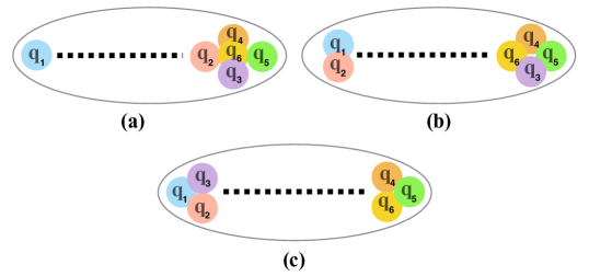
Figure 1: Different configurations of hexaquarks with n (=1,2,3) number of quark at one end of the string. There exists several combinations (6, 15, and 10) within those quarks for each of these three cases (a, b, and c respectively).

3 Results and discussion

The masses of quarks taken for the calculation are, $m_{up}=2.16MeV$, $m_{down}=4.67MeV$, $m_{strange}=93MeV$, $m_{charm}=1270MeV$ and $m_{bottom}=4180MeV$ respectively , and $K=0.2GeV^{2}$.[45] Here, $fc$ is the rotational speed of the low mass end of the string and $fc<1$. Here, the quarks and antiquarks that make up $q_{1}$ $q_{2}$, $q_{3}$ $q_{4}$, $q_{5}$, and $q_{6}$ are not stated explicitly. It is a general approach and one can consider any one as a quark or an antiquark. It will not have an impact on the formulae used here. In Table (3), calculated mass of different fully heavy hexaquark states are compared with other theoretical results. The mass of a hexaquark increases with decrease in the string length $l$ indicating the fact that, the QCD effect will be more for higher mass states. The speed also decreases for heavier states. There are few hexaquark states having same quark flavor. For states with same quark flavor, it is not necessary to consider the thirty one configurations as mentioned earlier. In Table (3) the calculated mass of hexaquark states having atleast one heavy quark are mentioned. We have considered different $l$ values for different states. We have found that the present results are in good agreement with other models. The trend in the results is similar to that obtained for the fully heavy hexaquark states. One of the noteworthy observation is that, the string length as well as rotational speed grows as we move to the state with a higher angular momentum. It is evident from the Regge trajectory equation that the angular momentum of a particle is proportional to the length of the string, while the mass squared is proportional to the tension of the string. Hence, as we are moving to the higher $J$ state, $l$ increases. Again, if the mass and distance from the center of rotation remain constant, as the speed rises, its orbital angular momentum will rise. This is due to the fact that orbital angular momentum is described by the equation $L=mvr$, where $m$ is the object’s mass, $v$ is its speed, and $r$ is its distance from the center of rotation. It is crucial to remember that the mass and distance from the center of rotation both have an impact on the relationship between orbital angular momentum and speed. For instance, the orbital angular momentum will increase if the object’s mass rises while its speed stays the same. It is clearly visible from the results given in both the tables that, for hexaquarks with heavy quark flavors, string length is very small. The length of the string for the heavy quark is expected to be shorter than that of a light quark, due to the relationship between quark mass, string tension, and string length in string theory. The intensity of the strong nuclear force, which holds quarks together, is correlated with the tension of the string, a fundamental constant of nature. A quark’s mass is determined by the energy stored in the string, which is related to the length and tension of the string. The energy held in the string increases as the mass of the heavy quark increases, in order to keep the same tension, the string’s length must be reduced. Fig. (2) shows the mass variation of hexaquarks with variation in speed $f$. It is almost same for all the hexaquark states and is highly non-linear. With increasing string length, the hexaquark mass variation rises linearly (Fig. 3). Variation of mass of hexaquark with speed $f$ and string length $l$ averaged for all possible configurations is depicted in Fig. 4. The calculated expression (Eq. 3; n=1) clearly demonstrates that the mass rises as the string length rises. Fig. (5) shows the Regge trajectories of different hexaquark states. It is found to be nonlinear. There are thirty-one hexaquark configurations in the flux tube model, and it is assumed that all the thirty-one configurations are equally probable. Hence the mass and angular momentum is averaged and the nonlinearity is obvious. Fig. (6) represents the Regge trajectories of hexaquarks made up of both light and heavy quarks. It demonstrates clearly how nonlinearity rises with heavier states. Fig. (7) shows the Regge trajectories of tetra, penta, and hexaquark states with all charm quark configurations. It is apparent from the figure that the Regge trajectories of tetraquark, pentaquark, and hexaquark are showing the same behavior.

Predicted masses of different hexaquark states SI. no. Quark $J$ M_cal $l$ $f$ Other structure ($MeV$) ($fm$) Results (See Ref.[29, 21, 22]) ($MeV$) 1 $cccccc$ 1 9526.39 0.11 0.709 $9490\pm 130$ 2 $cccccb$ 1 13214.81 0.08 0.740 13176 3 $ccccbb$ 1 16352.36 0.07 0.704 16373 4 $cccbbb$ 1 19119.56 0.065 0.657 19221 5 $ccbbbb$ 1 22029.22 0.06 0.613 22775 6 $cbbbbb$ 1 25106.67 0.052 0.612 25980 7 $bbbbbb$ 1 28090.95 0.049 0.560 $28500\pm 150$

Predicted masses of different hexaquark states SI. no. Quark $J$ M_cal $l$ $f$ Other structure ($MeV$) ($fm$) Results (See Ref.[46, 47]) ($MeV$) 1 $uuuuuc$ 1 3293.18 0.20 0.980 $\cdots$ 2 $uuuudc$ 1 3388.39 0.3 0.979 $\cdots$ 2 3858.41 0.2 0.987 3902 3 $uuuddc$ 1 3396.33 0.3 0.979 $\cdots$ 2 3868.37 0.2 0.989 3863 4 $uuuucc$ 1 4516.49 0.21 0.890 $\cdots$ 2 5125.59 0.30 0.919 5250 5 $uuudcc$ 1 4401 0.22 0.880 4420 2 4950.40 0.32 0.909 4911 6 $uuddcc$ 1 4304.43 0.23 0.870 4364 2 5032.48 0.31 0.914 5086 7 $uusscc$ 1 4814.71 0.19 0.903 $\cdots$ 8 $uscdsc$ 1 4841.12 0.18 0.907 $\cdots$ 9 $uuuccc$ 1 5892.87 0.16 0.887 $\cdots$ 10 $uuuudb$ 1 5996.24 0.9 0.768 5988 2 6926.28 0.88 0.891 6926 11 $uuuddb$ 1 6161.97 0.8 0.820 6142 2 6949.81 0.85 0.895 6928 12 $uucccc$ 1 7014.48 0.14 0.795 $\cdots$ 13 $uccccc$ 1 8049.02 0.13 0.766 $\cdots$ 14 $uuuubb$ 1 10202.13 0.14 0.675 10290 2 11628.24 0.17 0.795 11620 15 $uuudbb$ 1 11052.72 0.11 0.761 11395 2 11357.24 0.18 0.777 11372 16 $uuddbb$ 1 10707.07 0.12 0.731 10828 2 11359.88 0.18 0.777 11518

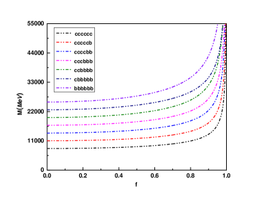
Figure 2: Mass variation (M) with change in speed $f$ of the hexaquarks.

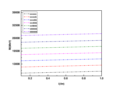
Figure 3: Mass variation (M) with change in string length $l$ of the hexaquarks.

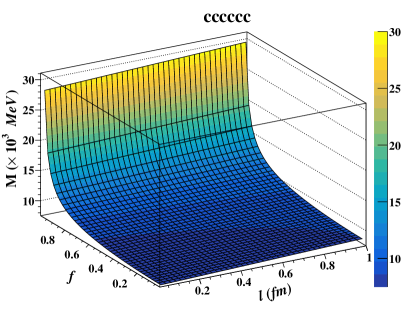
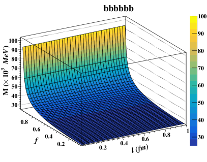
Figure 4: Mass variation with change in string length and fractional rotational speed for (a) $cccccc$, and (b) $bbbbbb$ hexaquark averaged for all possible (6+15+10) configurations of Fig. 1. Other hexaquarks also follows the similar pattern of gradual change in mass with change in string length.

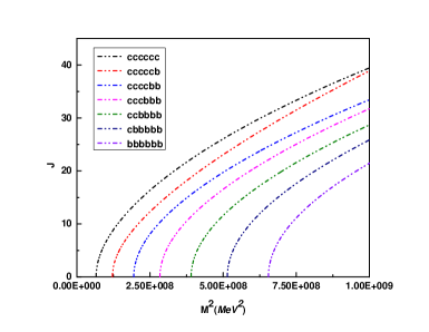
Figure 5: Regge trajectories for different hexaquarks.

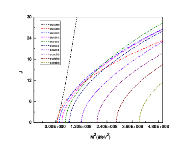
Figure 6: Comparison of Regge trajectories for light to heavy hexaquarks.

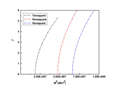
Figure 7: Regge trajectories for tetra, penta, and hexaquarks.

4 Conclusions and Future Prospects

In view of the results obtained, it is obvious to mark that the heavier states are accommodated with the string having shorter length. The masses of the hexaquark states are roughly linear when the rotational speed is low, but as the speed increases, they become significantly nonlinear. The Regge trajectories are largely linear for hexaquark states with the light quarks, but they become highly nonlinear for heavier states as evident from Fig. 6. We observed that the Regge trajectories for fully heavy tetraquark, pentaquark, and hexaquark states shows similar pattern (See Fig. 7). In order to fully comprehend the behavior and characteristics of the Regge trajectories of hexaquark states, additional theoretical and experimental research will be required for deeper insights. The detailed study of effects of string length on the hexaquark mass, breaking of flux tube, their relation with quark confinement, and emerging possibilities of dark matter sector are the topics beyond the scope of this work and we would like to address these issues in our future investigations.

References

- [1] F. Dyson and N. H. Xuong, Phys. Rev. Lett. 13, 815 (1964).
- [2] R. L. Jaffe, Phys. Rev. Lett. 38, 195 (1977).
- [3] M. Bashkanov, H. Clement and D. P. Watts, JPS Conf. Proc. 10, 021002 (2016).
- [4] P. Braun-Munzinger and B. Dönigus, Nuclear Physics A 987, 144-201 (2019).
- [5] P. Adlarson et al. (WASA-at-COSY Collaboration), Phys. Rev. Lett. 106, 242302 (2011).
- [6] P. Adlarson et al. (WASA-at-COSY Collaboration), Phys. Rev. C 88, 055208 (2013).
- [7] P. Adlarson et al. (WASA-at-COSY Collaboration), Phys. Lett. B 743, 325 (2015).
- [8] M. Bashkanov et al. (CELSIUS/WASA Collaboration), Phys. Rev. Lett. 102, 052301 (2009).
- [9] F. Kren et al. (CELSIUS/WASA Collaboration), Phys. Lett. B 684, 110 (2010), Erratum: Phys. Lett. B 702, 312 (2011).
- [10] M. Ablikim et al. Chinese Physics C 47, 043001 (2023).
- [11] J. Wu, Y. Liu, K. Chen, X. Liu and S. Zhu, Phys. Rev. D 97, 094015 (2018).
- [12] Z. Wang and Z. Di, Acta Phys. Pol. B 50, 1335 (2019).
- [13] X. Chen, Phys. Rev. D 100, 094009 (2019).
- [14] M. A. Bedolla, J. Ferretti, C. D. Roberts and E. Santopinto, Eur. Phys. J. C 80, 1004 (2020).
- [15] X. Jin, Y. Xue, H. Huang and J. Ping, Eur. Phys. J. C 80, 1083 (2020).
- [16] P. Lundhammar and T. Ohlsson, Phys. Rev. D 102, 054018 (2020).
- [17] G. Yu, Eur. Phys. J. C 83 416 (2023).
- [18] R. Aaij et al. (LHCb Collaboration), Sci. Bul. 65, 1983 (2020).
- [19] Y. Yan et al. Phys. Rev. D 105, 014027 (2022).
- [20] H. An et al. Phys. Rev. D 105, 074032 (2022).
- [21] Z. Wang, Int. J. Mod. Phys. A 37 2250166 (2022).
- [22] J.M. Alcaraz-Pelegrina and M. C. Gordillo, Phys. Rev. D 106, 114028 (2022).
- [23] F. Wang, G.H. Wu, L.J. Teng and T. Goldman, Phys. Rev. Lett. 69, 2901 (1992).
- [24] T. Goldman, K. Maltman, G.J. Stephenson Jr, J.-L. Ping and F. Wang, Mod. Phys. Lett. A 13, 59 (1998).
- [25] V.B. Kopeliovich, Nucl. Phys. A 639, 75 (1998).
- [26] Z.Y. Zhang, Y.W. Yu, X.Q. Yuan et al. Nucl. Phys. A 670, 178 (2000).
- [27] T. Kamae and T. Fujita, Phys. Rev. Lett. 38, 471 (1977).
- [28] K. Yazaki, Prog. Theor. Phys. Suppl. 91, 146 (1987).
- [29] Q. Lu, D. Chen and Y. Dong, arXiv:2208.03041 [hep-ph].
- [30] J. Cheng et al. Phys. Rev. D 107, 054018 (2023).
- [31] M. Loan, arXiv:0605005[hep-lat].
- [32] S. Amarasinghe et al. Phys. Rev. D 107, 094508 (2023).
- [33] K Azizi et al J. Phys. G: Nucl. Part. Phys. 47, 095001 (2020).
- [34] M. Bashkanov and D. P. Watts, J. Phys. G: Nucl. Part. Phys. 47, 03LT01 (2020).
- [35] M. G. Olsson, Nuov. Cim. A 107, 2541-2551 (1994).
- [36] K. Johnson, C. Nohl, Phys. Rev. D 19, 291 (1979).
- [37] N. Hothi and S. Bisht Indian J.Phys. 85, 1833-1842 (2011).
- [38] N. Hothi and S. Bisht, Electron. J. Theor. Phys. 10, 81 (2013).
- [39] R. Ghosh and A. Bhattacharya, Int. J. Theor. Phys. 56, 2335–2344 (2017).
- [40] J. Chen, Eur. Phys. J. A 57, 238 (2021).
- [41] J. Oudichhya, K. Gandhi and A. K. Rai, Phys. Scr. 97, 054001 (2022).
- [42] D. G. Sindhu, A. Ranjan, and H. Nandan Int. Jour. Mod. Phys. A 38, 2350044 (2023).
- [43] H. Nandan and A. Ranjan, Mod. Phys. Letts. A 27, 1250047 (2012).
- [44] A. Ranjan and H. Nandan, Int. J. Mod. Phys. A 31, 165007 (2016).
- [45] R. L. Workman et al. (Particle Data Group) Prog. Theor. Exp. Phys. 2022, 083C01 (2022).
- [46] S. M. Gerasyuta and E. E. Matskevich, Int. Jour. Mod. Phys. E 20, 2443-2462 (2011).
- [47] S. M. Gerasyuta and E. E. Matskevich, Int. Jour. Mod. Phys. E 21, 1250058 (2012).