Time-reparametrization invariance: from Glasses to toy Black Holes

Abstract

Glassy dynamics have time-reparametrization ‘softness’: glasses fluctuate, and respond to external perturbations, primarily by changing the pace of their evolution. Remarkably, the same situation also appears in toy models of quantum field theory such as the Sachdev-Ye-Kitaev (SYK) model, where the excitations associated to reparametrizations play the role of an emerging ‘gravity’. I describe here how these two seemingly unrelated systems share common features, arising from a technically very similar origin. This connection is particularly close between glassy dynamics and supersymmetric variants of the SYK model, which I discuss in some detail. Apart from the curiosity that this correspondence naturally arouses, there is also the hope that developments in each field may be useful for the other.

1 Introduction

Glasses are, by definition, systems that take very long - perhaps infinite - time to reach thermal equilibrium. It is natural then to try to understand the nature of such dynamics: is there something simple and generic that one can say about this physical situation, at least for the asymptotic limit in which relaxation becomes very slow, yet still far from equilibrium?

In this paper I concentrate on one such feature, that holds exactly in some solvable models, and at least to a good approximation in real systems: they develop an emergent time-reparametrization invariance: like a film that remains the same, but the speed at which it is projected is very weakly determined. Physically this means two things: i) small external perturbations may drastically alter the speed of evolution, and ii) spontaneous fluctuations of the ‘speed’ become large.

The first to note that reparametrization invariance emerged from a mean-field dynamical model were (to my knowledge) Sompolinsky and Zippelius 1982 [1]. Years later, the problem arose in the analytic solution of relaxation [2], mostly as a nuisance. Over the years, it was recognized that reparametrization softness explained the dramatic dynamical effect of driving a glass, for example with shear [3]. Later, in a remarkable series of papers, [4, 5, 6, 7], the spontaneous fluctuations of time-reparametrizations were studied, and a ‘sigma model’ for reparametrizations was proposed. Even the consistency of the Parisi ansatz for a finite-dimensional systems was recently argued to require the existence of reparametrization softness [8].

On a separate development, the quantum dynamics of certain fermion (Sachdev-Ye-Kitaev [9, 10]) models were shown to develop the same kind of invariance, and for exactly the same technical reasons, at low temperatures, when the imaginary time is large, and the dynamics become slow [9, 11, 12, 13, 10, 14, 15]. Reparametrizations embody the low energy properties of the system, and it was noted by Kitaev [10] that concentrating on these, one obtains a ‘toy’ version of how gravity and Black Holes emerge from a quantum field theory, saturating the expected bounds on chaos. Quite naturally, a sigma model of reparametrizations was developed [14] representing this.

That two rather similar routes would lead to an insight in two very different contexts inevitably arouses curiosity, and, from a practical point of view, suggests that technical tools could be exchanged. A preliminary exploration of this striking connection has been presented in Ref. [16].

2 Glassy dynamics, classical or quantum

2.1 Generics

Consider the glassy Hamiltonians [17, 18, 19]:

$$E_{p}=-\frac{1}{p!}\sum_{i_{1},...,i_{p}}J_{i_{1},...,i_{p}}q_{i_{1}}...q_{i_{p}}$$ (1)

where the $J_{i_{1},...,i_{p}}$ are independent random variables with variance $p!/2N^{p-1}$. We often build combinations of various $E_{p}$ with different $p$’s, that offer a palette of different behaviors. As it stands, the potential is unbounded. There are several ways to cure this: we may work with the $q_{i}$ being Ising or Potts variables, quantum or classical. For technical simplicity we choose the $q_{i}$ to be classical and constrained on a sphere $\sum_{i}q_{i}^{2}=N$. The dynamics could be anything that may be interpreted as a thermal bath at given temperature $T_{s}$: quantum or classical, Monte Carlo, Glauber, Heat Bath. Again, for technical simplicity we choose a classical Langevin process. Neither choice alters essentially the results of this paper. Indeed, the models we have defined contain most of what is relevant to an immense family of ‘hard’ computational problems, such as $k$-satisfiability, and graph coloring (see Fig. 1)

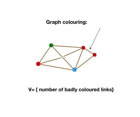
Figure 1: The Graph Coloring problem. The energy is the number of links joining equally colored vertices.

2.2 Four versions of slow dynamics

We consider then a system of $N$ coupled degrees of freedom $q_{i}(t)$ evolving by stochastic Langevin dynamics

$$\dot{q_{i}}(t)=-\frac{\partial V}{\partial q_{i}}+\eta_{i}(t)~{},$$ (2)

where $V$ is the interaction potential, $T_{s}$ the (classical) temperature of the thermal bath to which the system is coupled, and $\eta_{i}(t)$ is a Gaussian white noise with covariance $\langle\eta_{i}(t)\eta_{i}(t^{\prime})\rangle=2T_{s}\delta(t-t^{\prime})$. If we deal with spherical spins, we need to impose the constraint with a time-dependent Lagrange multiplier: $V=V_{o}+\lambda(t)[\sum_{i}q_{i}^{2}-N]$. Three correlations are important for the problem:

$$C(t,t^{\prime}) =\frac{1}{N}\sum_{i}\langle q_{i}(t)q_{i}(t^{\prime})\rangle~{},$$ (3)

$$R(t,t^{\prime}) =\frac{1}{N}\sum_{i}\langle q_{i}(t)\eta_{i}(t^{\prime})\rangle\;\;\;\;,\;\;\;\;\chi(t,t^{\prime})\equiv\int_{t^{\prime}}^{t}ds\;R(t,s)$$

$$D(t,t^{\prime}) =\frac{1}{N}\sum_{i}\langle\eta_{i}(t)\eta_{i}(t^{\prime})\rangle-2T_{s}\delta(t-t^{\prime})~{},$$

The average is over the dynamic process. We shall always understand $t\geq t^{\prime}$. For causal systems, since the noise is white, $D=0$.

Slow dynamics happen in different possible ways, even for the same system. Consider the following:

• Aging: Starting from a high temperature configuration, and connecting the system with a low-temperature bath, we find that it does not manage to equilibrate in observed times, or at all. We easily see this because correlations do not take the Time-Translational Invariant (TTI) form:

  $$C(t,t^{\prime})=C_{f}(t-t^{\prime})+\tilde{C}(t,t^{\prime})\;\;\;\;{\mbox{ for example}}=C_{f}(t-t^{\prime})+{\cal{C}}\left(\frac{t-t^{\prime}}{t^{\prime}}\right)$$

  so that the decay of correlation becomes slower as time passes. Furthermore, the Fluctuation-Dissipation Relation does not hold:

  $$\chi(t,t^{\prime})=\int_{t^{\prime}}^{t}dsR(t,s)\neq\beta[C(t,t)-C(t,t^{\prime})]$$

• Slowly evolving disorder: Suppose that in the low temperature phase, we make the disorder evolve very slowly, stochastically, so that:

  $$\langle J_{i_{1},...,i_{p}}(t)J_{i_{1},...,i_{p}}(t^{\prime})\rangle=p!/2N^{p-1}e^{-\frac{t-t^{\prime}}{\tau}}$$

  with $\tau$ large. Aging is suppressed, because the system adapts as best it can up to the timescale $\tau$, and then keeps ‘chasing’ the optimization with the changing couplings. A typical correlation may read:

  $$C(t,t^{\prime})=C_{f}(t-t^{\prime})+\tilde{C}(t,t^{\prime})\;\;\;{\mbox{ for example}}=C_{f}(t-t^{\prime})+{\cal{C}}\left(\frac{t-t^{\prime}}{\tau}\right)$$ (4)

  i.e. the system becomes stationary. However, it is not close to equilibrium. We know this because FDR is still violated, as we shall see.

• Weakly driven system: A very similar situation to the one above arises when the system has fixed disorder, but is driven by non-conservative forces: for example shear, or, in our toy models, an additional term in the equations of motion:

  $$\dot{q_{i}}(t)={\mbox{ usual terms }}+\frac{1}{\tau}\sum_{j}\;A_{ij}q_{j}$$ (5)

  with the matrix $A_{ij}$ non-symmetric, constant and dimensionless. Driving the system, however weakly, keeps it from aging, beyond a point.

• Breaking causality: We may impose that the trajectory starts and ends in given configurations ${\bf q}_{i}$ and ${\bf q}_{f}$, at times zero and $\tau$, respectively. This may force the system to cross barriers, for example. We shall also be naturally led to considering ${\bf q}_{i}={\bf q}_{f}$

In the aging case, the dynamics becomes slow when the smallest time $t^{\prime}$ becomes large, a self-generated large parameter. In all other cases, the chosen timescale $\tau$ is the large parameter.

2.3 Solution for large $N$

The solution for this problem may be obtained by summing dominant diagrams (usually in the field theory community), or by writing a path integral version of the dynamics and averaging (always, in the glass community). The situations above are just chosen by fixing the boundary conditions in time. Only the causality-breaking situation requires, in principle, to replicate the dynamics, because the normalization is no longer unity in that case. One obtains then, in terms of $C,R,D$ a weight of the form $e^{-NS[C,R,D]}$, which leads, after variation, to the equations of motion, exact in the large-$N$ limit:

$$\left(\frac{d}{dt}-2T{\bf U}\right){\bf Q}(t,t^{\prime})=\int ds\;{\bf\Sigma}(t,s){\bf Q}(s,t^{\prime})-\mbox{\boldmath$\lambda$}(t){\bf Q}(t,t^{\prime})+\mbox{\boldmath$\delta$}(t-t^{\prime})$$ (6)

with the definitions:

$${\bf Q}=\begin{bmatrix}R&C\\ D&R^{t}\end{bmatrix}(t,t^{\prime})\;\;,\;\;\mbox{\boldmath$\delta$}=\begin{bmatrix}\delta&0\\ 0&\delta\end{bmatrix}(t-t^{\prime})\;\;,\;\;\mbox{\boldmath$\lambda$}=\begin{bmatrix}\lambda&0\\ -\hat{\lambda}&\lambda\end{bmatrix}(t)\;\;,\;\;{\bf U}=\begin{bmatrix}0\;&\;1\\ 0\;&\;0\end{bmatrix}$$ (7)

$${\bf\Sigma}=p\begin{bmatrix}(p-1)C^{p-1}R\;\;&\;\;C^{p-1}\\ (p-1)C^{p-2}D+(p-1)(p-2)C^{p-3}R\;\;&\;\;(p-1)C^{p-1}R^{t}\end{bmatrix}(t,t^{\prime})$$ (8)

The reader familiar with the SYK model will recognize the similarity .

In the glass literature, it is customary to separate explicitly the fast and the slow relaxations, which occur at small and large time-differences, respectively.

$$\;\;\;C(t,t^{\prime}) =C_{f}(t-t^{\prime})+\tilde{{C}}\left(t,t^{\prime}\right)~{},$$ (9)

$$\;\;\;R(t,t^{\prime}) =R_{f}(t-t^{\prime})+\tilde{{R}}\left({t,t^{\prime}}\right)~{},$$

$$\;\;\;D(t,t^{\prime}) =D_{f}(t-t^{\prime})+\tilde{{D}}\left({t,t^{\prime}}\right)~{},$$

If we separate the fast relaxations, for the remaining ‘slow’ parts, the time-derivatives become small, in terms of $t^{\prime}$ in the aging case, and in terms of the parameter $\tau$ in the other three cases. In that limit, we may drop the l.h.s. of (8), and the rest obeys a reparametrization invariance,
$\displaystyle\;\;\;\tilde{C}(t,t^{\prime})$ $\displaystyle\rightarrow\tilde{C}(h(t),h(t^{\prime}))~{},$ $\displaystyle\;\;\;\tilde{R}(t,t^{\prime})$ $\displaystyle\rightarrow\dot{h}(t^{\prime})\;\tilde{R}(h(t),h(t^{\prime}))~{},$ $\displaystyle\;\;\;\tilde{D}(t,t^{\prime})$ $\displaystyle\rightarrow\dot{h}(t)\dot{h}(t^{\prime})\;\tilde{D}(h(t),h(t^{\prime}))$         and     $\displaystyle\lambda(t)$ $\displaystyle\rightarrow\lambda(h(t))~{},$ (10) $\displaystyle\hat{\lambda}(t)$ $\displaystyle\rightarrow\dot{h}(t)\;\hat{\lambda}(h(t))$  

Note that the anomalous dimension is zero, in this case [20]. This pseudo invariance has an important physical meaning for glasses, as we shall see in the next section.

3 Physical consequences

In the aging case, if one makes a parametric plot of integrated response $\chi(t,t^{\prime})$ versus $C(t,t^{\prime})$, one finds that for large $t^{\prime}$ the curves collapse into one, sketched in Fig. 2. If the Fluctuation-Dissipation relation were to hold, one would obtain a straight line with gradient $-\beta$. But we are out of equilibrium here, so the FDR does not apply. The result is however surprising: one obtains two straight lines, one - corresponding to small time-differences - is the one we would have obtained in equilibrium, while the other has the form we would have at another temperature $\beta_{\mathrm{eff}}$ , self-generated by the system. The emergence of an effective temperature $\beta_{\rm{eff}}$ will be further discussed in Section 7.

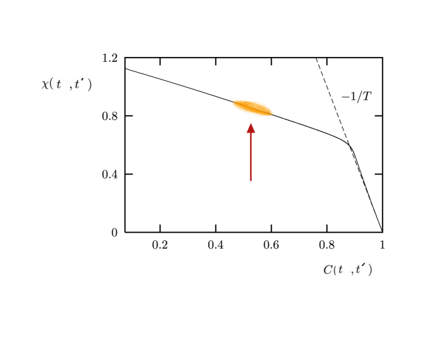
Figure 2: The Fluctuation-Dissipation plot breaks into two lines, one with gradient $\beta$ - as one would have in equilibrium - corresponding to fast relaxations, and one with a self-generated $-\beta_{\mathrm{eff}}$, corresponding to slow relaxations (see Ref. [21]). Thermal fluctuations are large along the line, small in transverse directions.

Next, we consider the cases of a slowly evolving disorder, or with weak drive. In both these situations, the system becomes stationary (only dependent on time-differences), just like a system in equilibrium. What happens with the $\chi$ vs. $C$ plot then? Quite surprisingly, it is identical to the one for the aging case, underlining the fact that we are stationary but still out of equilibrium. What has happened is that both the slow evolution of disorder, and the weak drive, have dramatically reparametrized the time, changing completely the form of the slow part of the relaxation. We should indeed not be surprised about this fact, since time-reparametization is almost an invariance. The long time limit of $\chi(C)$ is instead a reparametrization invariant object, and stays stable. The situation is as in Fig. 3: time-dependencies are like the angle in this simple example, while reparametrization invariant quantities are like the radius.

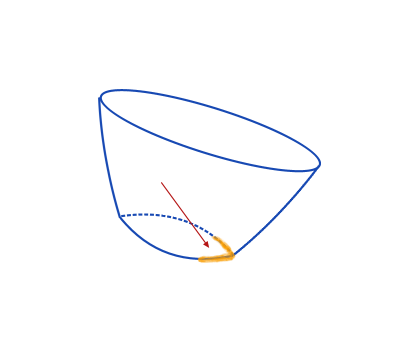
Figure 3: A quasi-symmetry. The thermal fluctuations are large along the ‘angles’.

Another reparametrization invariant quantity is constructed as follows [22]: i) choose a large time $t^{\prime}$ and a subsequent time $t$ such that the correlation $C(t,t^{\prime})$ takes a small fixed value, say $C=.1$. ii) For all $t^{\prime}<s<t$, plot $C(t,s)$ versus $C(s,t^{\prime})$. iii) repeat for larger $t^{\prime}$ (in aging, or larger $\tau$ in the other cases) Again, this plot is the same whatever the precise time-reparametrization (see Fig. 4).

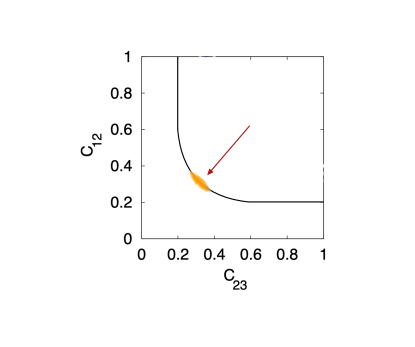
Figure 4: A reparametrization invariant plot involving three correlations. In orange, a sketch of fluctuations of different realizations.

In the series of papers mentioned above[4, 5, 6, 7], the authors studied how spontaneous fluctuations of realistic systems are seen in a reparametrization-invariant plot such as Fig 2 and Fig 4, and indeed found that they tend to concentrate along the lines, as shown in orange (artist view) in these two figures: indeed, an experimental version of Fig. 3.

Reparametrization invariance also plays a crucial role in the activated processes in glasses. In a remarkable paper [23], Rizzo considered the situation in which initial and final states are deep, equilibrium states, and there is a passage from one to the other in time $T$. Interestingly, the ‘slow’ parts of the solutions for given passage times $T$, are time-reparametrizations of one another

$$C(t,t^{\prime}) =C_{f}(t-t^{\prime},t/T)+{\cal{C}}\left(\frac{t-t^{\prime}}{T}\right)~{},~{}$$ (11)

$$R(t,t^{\prime}) =R_{f}(t-t^{\prime},t/T)+\frac{1}{T}{\cal{R}}\left(\frac{t-t^{\prime}}{T}\right)~{},$$

$$D(t,t^{\prime}) =D_{f}(t-t^{\prime},t/T)+\frac{1}{T^{2}}{\cal{D}}\left(\frac{t-t^{\prime}}{T}\right)~{},$$

$$\lambda(t) =\ell\left(\frac{t}{T}\right)~{}\;\;\;,\;\;\hat{\lambda}(t)=\frac{1}{T}\;\hat{\ell}\left(\frac{t}{T}\right)~{},$$

The consequences of this finding have not yet been completely fleshed out.

4 SYK

Here I will be brief, as the subject is treated in Sachdev’s contribution in the same issue. The Hamiltonian of the Sachdev–Ye–Kitaev model reads

$$H_{syk}={({\mathrm{i}})^{\frac{q}{2}}}\sum_{1\leq i_{1}<\dots<i_{q}\leq N}J_{i_{1}...i_{q}}\chi_{i_{1}}...\chi_{i_{q}}~{},$$ (12)

where $\chi_{i}$ are $N$ Majorana fermions. The couplings $J_{i_{1}...i_{q}}$ are independent, identically distributed Gaussian random variables with zero mean and variance $N^{1-q}J^{2}(q-1)!$.

In order to study the thermodynamics, one has to compute

$$\overline{\ln Z}=\overline{\ln{\mathrm{tr}}\left[e^{-\beta H_{syk}}\right]}~{},$$ (13)

where the overbar denotes an average over the couplings. This is usually done by replicating the system $n$ times and then continuing to $n\rightarrow 0$. It turns out, however, that due to the Grassmannian nature of the degrees of freedom and the lack of a glass transition, order parameters coupling different replicas vanish, and the result coincides with the annealed average,

$$\ln\overline{Z}=\ln\overline{{\mathrm{tr}}\left[e^{-\beta H_{syk}}\right]}~{}.$$ (14)

Following precisely the same steps as in the mean-field glass, we obtain a result exact in the large $N$ limit

$$\ln\overline{Z}=\ln\int D[G]e^{-NS[G]}~{},$$ (15)

in terms of the correlation:

$$G(t-t^{\prime})=\sum_{i}\langle T\chi_{i}(t)\chi_{i}(t^{\prime})\rangle~{}.$$ (16)

The large $N$ limit allows for a saddle point evaluation, and one finds that the saddle-point value of $G$ satisfies the following equation

$${\frac{\partial G(t_{1},t_{2})}{\partial{t_{1}}}}=J^{2}\int_{0}^{\beta}dt\ G(t,t_{2})^{q-1}\;G(t_{1},t)\ +\delta(t_{1}-t_{2})~{}.$$ (17)

The reader familiar with Dynamical Mean Field solutions, will recognize the similarity.

The large $t$ solution of (17), for $T\rightarrow 0$, is  [11, 10, 14, 15, 24]

$$G(t_{1},t_{2})\propto\frac{1}{|t_{1}-t_{2}|^{{2}/{q}}}{\mathrm{sign}}(t_{1}-t_{2}),$$ (18)

The effect of a a small, positive temperature, is to cut off the critical power law behavior, at a timescale of the order of $\beta$. The specific heat is linear at low temperature and, more important for us here, the model displays a positive zero-temperature entropy.

Just as in the glassy case, the equation (17) has, to the extent that we may neglect the time-derivative term, the approximate reparametrization invariance:

$$G(t_{1},t_{2})\rightarrow|\dot{h}(t_{1})\dot{h}(t_{2})|^{1/q}G(h(t_{1}),h(t_{2}))~{}.$$ (19)

Of course, only one specific parametrization corresponds to the true minimum of the action. As noted by Parcollet and Georges [11], one can obtain the low-temperature behavior from the zero-temperature one through a reparametrization: $t_{a}\rightarrow\tan\left(\frac{\pi t_{a}}{\beta}\right)$ ($a=1,2$) which maps (18) into a time-translational invariant function of period $\beta$,

$$G_{\beta}(t_{1}-t_{2})=b\left[\frac{\pi}{\beta\sin\frac{\pi(t_{1}-t_{2})}{\beta}}\right]^{2/q}{\mathrm{sign}}(t_{1}-t_{2}),$$ (20)

The breaking of reparametrization invariance, which is a continuous symmetry, leads to the emergence of almost-soft modes governing low temperature fluctuations. An effective theory for reparametrizations was constructed explicitely [14]: it allows one to compute all the low-energy properties including the main critical fluctuations, which corresponds to four-point functions, in particular those related to the quantum Lyapunov exponent—extracted from the so called out-of-time-order correlation function (OTOC). This is Kitaev’s intuition [10]: the theory based on $S[h]$ has many of the symptoms one expects from a toy version of quantum gravity.

5 Bringing together the two situations

We wish to establish a relation between glassy dynamics (classical or quantal), with the quantum SYK model, in both of which the main role is played by an emerging reparametrization quasi-invariance. The connection we discuss here is not made through quantizing the original glass model, since reparametrization is for glasses already present in classical dynamics. Indeed, it comes with a twist:

The evolution of the probability density following equation (2) is generated by the Fokker–Planck operator $H_{\textrm{FP}}$,

$$\partial_{t}P_{t}(\mathbf{q})=\sum_{i}\frac{\partial}{\partial q_{i}}\left[T_{s}\frac{\partial}{\partial q_{i}}+\frac{\partial V}{\partial q_{i}}\right]P_{t}(\mathbf{q})\equiv-H_{\textrm{FP}}P_{t}(\mathbf{q}).$$ (21)

The Fokker–Planck operator is not Hermitian, but detailed balance is satisfied with the Gibbs distribution

$$e^{V/T_{s}}H_{\textrm{FP}}e^{-V/T_{s}}=H_{\textrm{FP}}^{\dagger}~{}.$$ (22)

This allows us to write it in an explicitly Hermitian form [25, 26]. Rescaling time, one can define the operator

$$H=\frac{T_{s}}{2}e^{V/2T_{s}}H_{\textrm{FP}}e^{-V/2T_{s}}=\sum_{i}\left[-\frac{T_{s}^{2}}{2}\frac{\partial^{2}}{\partial q_{i}^{2}}+\frac{1}{8}\left(\frac{\partial V}{\partial q_{i}}\right)^{2}-\frac{T_{s}}{4}\frac{\partial^{2}V}{\partial q_{i}^{2}}\right]\$$ (23)

$H$ has the form of a Schrodinger operator with $T_{s}$ playing the role of $\hbar$, unit mass and potential

$$V_{{\mathrm{eff}}}=\frac{1}{8}\sum_{i}\left(\frac{\partial V}{\partial q_{i}}\right)^{2}-\frac{T_{s}}{4}\sum_{i}\frac{\partial^{2}V}{\partial q_{i}^{2}}~{}.$$ (24)

The spectrum of $H_{\textrm{FP}}$ and that of $H$ are the same, up to the rescaling in (23), and the eigenvectors are related via the transformation above.

The connection we establish is the following: we shall consider $H$ as our (formally) ‘quantum’ Hamiltonian. Its partition function $Z=\mathrm{tr}e^{-\beta_{q}H}$ is obtained by introducing a quantum temperature $\beta_{q}$ . Then, $T_{s}$ we interpret as a parameter playing the role of $\hbar$, (not the quantum temperature). A we shall see, $H$ has a quantum phase transition at $T_{q}=0$ and the value of $T_{s}$ in which the original system had a dynamic glass transition $T_{s}=T_{\mathrm{mct}}$. What may be confusing is that, although the original system, whose partition function is $Z_{c}={\mathrm{tr}}\;e^{-\beta_{s}V}$ will have replica symmetry breaking at low temperature $T_{s}$, the ‘quantum’ system $Z=\mathrm{tr}\;e^{-\beta_{q}H}$ need not.

We can infer the spectral properties of $H$ from the general connection between spectra and metastability [27, 28]. Consider first a low-temperature $T_{s}$ Langevin process on the potential $V$ of Figure 5. It contains two metastable and a stable state. It is intuitive, and may be shown [27, 29, 28] that the spectrum of its Fokker-Planck operator has three low energy eigenstates, of eigenvalue the inverse of the lifetime of the corresponding metastable states in the original system - zero, if they are fully stable. Furthermore, their wavefunctions are combinations of the localized, positive, distributions within each state - see Fig 5. This is a completely general fact, and is independent of the actual origin of metastability, be it low temperature or, as in our case here, large $N$.

When we compute $Z=\mathrm{tr}\;e^{-\beta_{q}H}$ we are in fact summing over trajectories following a Langevin equation (2) but that, due to a lucky realization of the noise $\eta_{i}(t)$, they turn out to be periodic with period $\beta_{q}$.

In the case of our model glass, the situation is depicted in Figs. 6 and 7: We know from the theory of these models that there is an exponential number of metastable states with lifetimes diverging with $N$, corresponding to an exponential number of vanishing eigenvalues of $H$. Its zero $T_{q}$ entropy is then precisely the logarithm of this number. The argument may be generalized to barriers and the supersymmetric extension, we shall come back to this in Sect 8.

Suppose that we are at a stochastic temperature $T_{s}$ such that the system with potential $V$ is in a glassy phase, and replica symmetry is broken when we evaluate ${\mathrm{tr}}\;e^{-\beta_{s}V}$ When we compute instead $Z=\mathrm{tr}\;e^{-\beta_{q}H}$, we are looking for trajectories that close and are probable: for this we need that they are in the inside of states whose lifetime is not much shorter than $\beta_{q}$. So we need to look for where are the most numerous of these: it turns out that they are just above the threshold level on figure 6 (right), see dashed line of figure 7. For larger $\beta_{q}$, trajectories have to be inside less numerous but more stable metastable states, eventually concentrating on the threshold level of figure 7. This situation need not necessarily be accompanied by a transition in $\beta_{q}$, as we shall see in section 8.2.

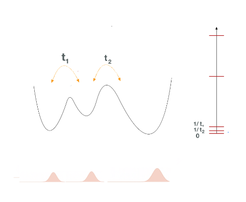
Figure 5: Localized wavefunctions of the form $\langle x|a\rangle\propto e^{-\beta V}\Theta(a)$, where $\Theta(a)$ is one in the region of the basin a and zero elsewhere. Eigenstates of $H$ are proportional to these, eventually hybridized. Note that as they are drawn, they are approximately orthogonal – because they are localized – and positive. It can be shown that the exact ‘low’ eigenstates may always be de-hybridized into a set of these approximately positive and orthogonal vectors.

The direct connection is then as in Figure 6, and holds for the dynamics of any glass model, classical or quantum (in the latter case the spectrum considered is the one of the Lindbladian): the set of metastable states constituting the glass correspond to low eigenvalues of $H$ dominating $T_{q}\rightarrow 0$, and play the same role of the states representing the ‘Black Hole’ in SYK. The detailed description in both cases is encoded in a theory for the reparametrizations.

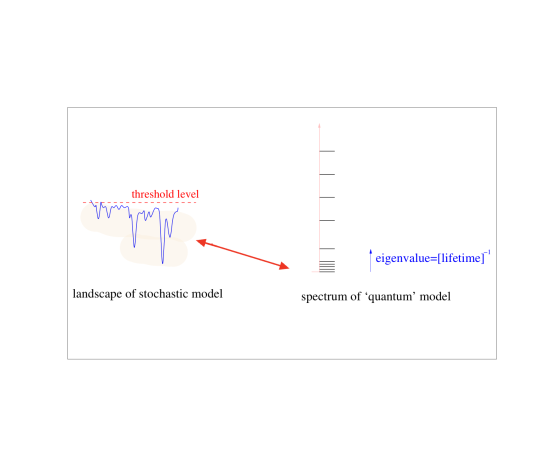
Figure 6: Spectral properties of the stochastic evolution, our ‘quantum’ Hamiltonian, and its correspondence to metastable states of the glass.

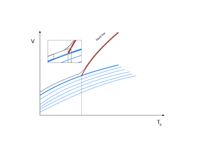
Figure 7: A sketch of the energy landsdcape as a function of the stochastic temperature. In blue, the glassy states sitting around minima of the potential, their number grows exponentially for higher $V$, until at a certain point they become unstable. At higher $V$ the number of saddles keeps increasing, but they are no longer minima, their typical index grow with their value of $V$. The intersection with the liquid line marks the dynamic transition $T_{s}$.

Let us note that again that $H$ corresponds to supersymmetric quantum dynamics restricted to the subspace of zero fermions. The connection between this and other supersymmetric SYK-like variants will be outlined in Section 8.

6 The classical glass dynamic transition as a ‘quantum’ critical point

6.1 The special $p=2$ case

In Ref [16], the $p=2$ version of the dynamics with potential Eq (1) were obtained, and are summarized in Table 1). This case is not quite a glass because it does not have many metastable states, but it is nice because it may be easily solved, and it has some interesting properties. The original model has a transition at $T_{s}=T_{c}$. Considered as a quantum model, and evolving in real time, at and below the transition $T_{s}\leq T_{c}$ the correlation first decays as

$$C(t)=q+\frac{b}{t^{\frac{1}{2}}}\ .$$ (25)

into a plateau of value $0<q<1$. Then it relaxes from $q$ to zero, in a timescale that diverges as $\tau\sim\beta_{q}^{2}$ for $T_{s}<T_{c}$, but is Planckian at exactly $T_{c}=T_{q}$, i.e. $\tau\sim\beta_{q}$, and is short when $T_{s}>T_{c}$ (see Table 1).

From the point of view of the associated ‘quantum’ Hamiltonian $H$, the specific heat displays a non-trivial scaling for $T_{q}\rightarrow 0$.

Table 1: Summary of results for $p=2$.

	$T_{s}<T_{c}$	$T_{s}=T_{c}$	$T_{s}>T_{c}$
$q$	$1-T_{s}/T_{c}$	0	0
specific heat	$T_{q}^{3/2}$	$T_{q}^{3/2}$	$e^{-\frac{{1}}{2}(T_{s}-T_{c})^{2}\;\beta_{q}}$
dynamics	Plateau $q+\frac{b}{t^{\frac{1}{2}}}$ for $t\ll\beta_{q}^{2}$	$\frac{b}{t^{\frac{1}{2}}}$ for $t\ll\beta_{q}$	$e^{-i\frac{(T_{s}-T_{c})^{2}\;t}{2T_{s}}}/t^{3/2}$

The vanishing of the $T_{q}=0$ quantum entropy is directly related to the non-exponential number of metastable states in the $p=2$ model. In order to obtain a different result one has to consider classical models with a much rougher energy landscape. This is what we do in the following focusing on $p>2$.

6.2 Glassy systems with $p>2$ terms

The classical system of energy given by (1) has a transition at the classical temperature $T_{s}=T_{\mathrm{mct}}$. The organization of states is sketched in Figs 6 and 7 (for $p>2$). At low energies $V$ there are many metastable states whose lifetime is exponential in $N$. At given $T_{s}$ their number increases exponentially with $V$, up to a point above which they lose their stability, i.e. their lifetime $\tau(V,T_{s})$ becomes finite . The higher the $V$, the shorter the lifetime, but the number of such states keeps increasing exponentially. For $T_{s}>T_{\mathrm{mct}}$ the liquid phase dominates the dynamics (the liquid line in Fig 7), but many metastable states also survive above $T_{\mathrm{mct}}$ for an additional temperature interval: these are not relevant for the dynamics. The actual dynamics we are interested in follows the dashed line in Fig. 7, it is in equilibrium above $T_{\mathrm{mct}}$ and out of equilibrium below.

In order to follow the physical situation, and to get rid of ambiguities, we shall consider the (slightly) modified Hamiltonian:

$$H_{\mu}=H+\mu V$$ (26)

The extra term reweights every state with a additive small quantity $=\mu\langle V\rangle_{state}$, which guarantees that ${\mathrm{tr}}e^{-\beta_{q}H_{\mu}}$ is dominated by the dashed line level in Fig 7. Considered as a ‘quantum’ system, the partition function ${\mathrm{tr}}\;e^{-\beta_{q}H_{\mu}}$ has a ‘quantum’ transition only in the limit $\mu\rightarrow 0$, between a situation with a finite entropy at $T_{q}=0$ when the parameter $T_{s}<T_{\mathrm{mct}}$ and zero when $T_{s}>T_{\mathrm{mct}}$. The transition point is then ($T_{s}=T_{\mathrm{mct}}$ , $T_{q}=0$, $\mu\rightarrow 0$). This point corresponds to the so-called ‘Mode Coupling Transition’ of glass theory [31, 32], hence the notation $T_{\mathrm{mct}}$.

The complete solution of this problem is yet to be done, see Refs [28, 16] for partial results. A rather crude argument (see inset in Fig 7) gives interesting hints: consider a situation in which $T_{s}$ is just below $T_{\mathrm{mct}}$, and we fix through a small value of $\mu$ the value ${\cal{V}}_{\mu}=\langle V\rangle_{\mu}$. Then $\varepsilon\equiv({\cal{V}}_{\mu}-{\cal{V}}_{0})$ is correspondingly small. The main assumption is to estimate the timescale $\tau$ of the correlation decay as being the same as the one in equilibrium at the temperature $T_{s}>T_{\mathrm{mct}}$, such that the liquid energy is $\varepsilon$ above the highest glass energy, the argument being that the metastable states contributing to the dynamics are the same. From Mode Coupling Theory, we know that $\tau\propto(T_{s}-T_{\mathrm{mct}})^{-\gamma}$ where $\gamma$ is a mode-coupling exponent. The extensive eigenstates of $H_{\mu}$ contributing to this are of order $\epsilon\sim\tau^{-1}$ per degree of freedom, while the log of the number of metastable states of this value is just linear in $S\propto\beta_{\mathrm{eff}}\;\varepsilon$, where $\beta_{\mathrm{eff}}$ is a constant. Again $T_{s}-T_{\mathrm{mct}}$ and $\varepsilon$ are proportional, so $\tau\propto\varepsilon^{-\gamma}$. With these assumptions, we may determine $\varepsilon$ in terms of the saddle point in the exponent $Z=Z_{0}\;e^{N[\beta_{\mathrm{eff}}\varepsilon-b\beta_{q}\varepsilon^{-\gamma}]}$, to obtain $T_{q}=T_{\mathrm{eff}}b\gamma\varepsilon^{\gamma-1}$. From this, we get an estimate of the timescale:

$$\tau\propto\left(\frac{\beta_{q}}{\beta_{\mathrm{eff}}}\right)^{\frac{\gamma}{\gamma-1}}$$ (27)

Remarkably, $\gamma$ is known to be $1\leq\gamma\leq\infty$ [33, 32]. In fact, one may tune it to any value in this range, just by playing with combinations of the terms $E_{p}$ in (1). This means that the timescale is always longer than Planckian. This suggests that in imaginary time, we should not expect to see any descent away from the plateau value $q$ (Matsubara time is never long enough). $q$ is the ‘size’ of the state. The scale would only become Planckian as $\gamma\rightarrow\infty$: a value in the parameters that has a precise meaning: it is a triple point where the transition of the original glass stops being from replica symmetric to one-step replica symmetry breaking, and becomes replica-symmetric to full replica symmetry- breaking (see Ref. [34]): the whole organization of saddle points in the landscape changes there.

Even if this argument is tentative, it points out that something interesting may happen at that triple point of $V$.

7 Coupling two systems: thermo-field double

As mentioned above, a property of slow dynamics in a model given by Eq. (1) is that when kept out of equilibrium in any of the ways described in Section 2 we obtain a fluctuation-dissipation plot as in Fig. 2, where an effective temperature $\beta_{\mathrm{eff}}$ emerges. The reason for this was unexpected [2, 21] and is non-trivial: the slow dynamics explores metastable states in a ‘democratic way’ so that the measure is, for all practical purposes

$$|TF\rangle\propto\sum_{a}e^{-\frac{1}{2}\beta_{\mathrm{eff}}F(a)}|a\rangle$$

where $F(a)$ is the free energy (at temperature $T_{s}$) restricted to state ‘$a$’ of ‘size’ $q$:

$$q=\frac{1}{N}\sum_{i}\langle a|q_{i}|a\rangle^{2}/\langle a|a\rangle^{2}$$

the Edwards-Anderson parameter. Here, as discussed in Section 5 (see Fig. 5), each low-lying state is of the form $\langle x|a\rangle\propto e^{-\frac{\beta}{2}V(x)}\Theta(a)$, where $\Theta(a)$ has support in $a$. (The $1/2$ factor in the exponent comes from the transformation Eq. (23), and thus corresponds to a Gibbs-Boltzmann distribution)

Two temperatures appear: the bath one inside the state, and the other one $\beta_{\mathrm{eff}}$ that reflects the choice of the metastable states explored by the nonequilibrium dynamics.

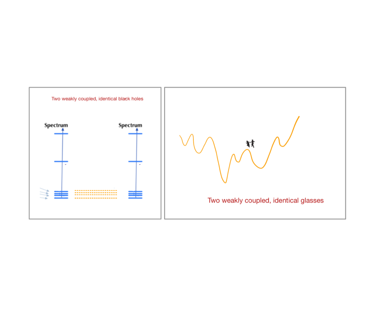
Figure 8: Weakly coupled walkers explore the same state at each time, but independently inside it.

Consider now two systems with the same energy given by Eq. (1), kept out of equilibrium in the same way as before (see Sect. 5.2 of Ref [8]). If the systems are uncoupled, the dynamics follow their own paths, and the overlap between systems is zero. Instead, if we couple the systems just strongly enough in a way as to favor them moving near each other (Fig. 8)

$$V^{(2)}=-\frac{1}{p!}\sum_{i_{1},...,i_{p}}J_{i_{1},...,i_{p}}\left\{q_{i_{1}}...q_{i_{p}}+q_{i_{1}}^{\prime}...q_{i_{p}}^{\prime}\right\}+\epsilon\sum_{i}q_{i}q_{i}^{\prime}$$ (28)

the systems will be having their fast evolutions independently, but at all times within the same state, i.e. they ‘jump together’. For exactly the same reasons as for two coupled SYK models, in the limit of slow dynamics, the coupling needed to keep the systems in pace becomes small in the limit of large $\tau$, their fast motion is uncoupled, while the slow motion is coupled – the infrared is coupled while the ultraviolet is not. Because metastable states are then ‘locked’ to be in the same basin for both systems, the eigenstates are then of the form

$$|aa\rangle=|a\rangle_{1}\otimes|a\rangle_{2}$$ (29)

or hybridizations thereof. [35] Again, to a good approximation this means that the distribution is

$$|TFD\rangle\propto\sum_{a}e^{-\beta_{\mathrm{eff}}F(a)}|aa\rangle$$ (30)

so we discover that the coupled slow dynamic is naturally represented by the thermo-field double, in a way that is very reminiscent of the construction in Ref. [35]. Let us remark in passing that making two replicas evolve together is actually a good practical method for optimization, see Ref [36])

8 Supersymmetric models as glassy dynamics

8.1 Hamiltonians

As we mentioned above, $H$ may be promoted to full SUSY quantum mechanics by adding fermions:

$$H_{\mathrm{susy}}=H+\frac{T_{s}}{2}\sum_{ij}\frac{\partial^{2}V}{\partial q_{i}\partial q_{j}}a^{\dagger}_{i}a_{j}$$ (31)

We may equivalently write this in the base of the Fokker-Planck operator

$$H_{{\mathrm{FP-susy}}} = -\sum_{i}\frac{\partial}{\partial q_{i}}\left[T_{s}\frac{\partial}{\partial q_{i}}+\frac{\partial V}{\partial q_{i}}\right]+\frac{T_{s}}{2}\sum_{ij}\frac{\partial^{2}V}{\partial q_{i}\partial q_{j}}a^{\dagger}_{i}a_{j}$$ (32)

$$= -\sum_{i}P_{i}\left[T_{s}P_{i}+\frac{\partial V}{\partial q_{i}}\right]+\frac{T_{s}}{2}\sum_{ij}\frac{\partial^{2}V}{\partial q_{i}\partial q_{j}}a^{\dagger}_{i}a_{j}$$

where $P_{i}\equiv\frac{\partial}{\partial q_{i}}$ .

The zero-fermion subspace anihilated by $a_{i}$ represents the Fokker-Planck equation, which in turn derives from the Langevin Eq (2). We may choose the fermion number $N_{f}=\langle\sum a^{\dagger}_{i}a_{i}\rangle$ subspace directly, or by adding a chemical potential $H_{\mathrm{susy}}+zN_{f}$ in the Hamiltonian. If $z=0$ , typically half-filled $N_{f}\sim N/2$ subspaces dominate, because those saddles are overwhelmingly more numerous in a disordered system.
$\bullet$ Physical glasses are about the $N_{f}=0$ subspace, although the theory gives us indications on higher $N_{f}$ as well.
$\bullet$ To the best of my knowledge supersymmetric models have been studied (except for a brief mention in Ref [30]) without fixing the fermion number, which usually amounts to being dominated by half-filling.

Metastable states are then generalized to the case with fermions (31) : low $k$-fermion eigenstates are concentrated on barriers of index $k$ (see Fig. 9), and one may in general reproduce the construction for Morse theory [39], again generalized to any possible origin of the metastability other than low temperature [38], most notably large $N$.

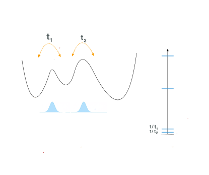
Figure 9: Same as in Fig. 5, but for one-fermion states of $H_{\mathrm{susy}}$. ‘Barrier states’ are like metastable states, but with $k$ unstable directions.

Let us compare this to a family of supersymmetric models in the literature [40, 41] - here we follow the notation of Ref [30].

$N=2$

$$S = S_{f}+S_{f}$$ (34)

$$S_{b} = \int d\tau\;\;\left[\frac{1}{2}(\dot{\phi}_{i})^{2}+\frac{1}{2}(F^{i})^{2}+3iC_{ijk}F^{i}\phi^{j}\phi^{k}\right]$$

$$S_{f} = \int d\tau\;\;\left[\delta_{\alpha\beta}\delta_{jk}\frac{\partial}{\partial\tau}+3iC_{ijk}F^{i}\right]\psi_{\alpha}^{j}\phi_{\beta}^{k}$$ (35)

Let us make the change of variables $P_{i}=iF_{i}+\dot{\phi}$. We obtain, up to a boundary term (i.e. we are making a canonical transformation):

$$S_{b}=P_{i}\dot{\phi}_{i}-\frac{1}{2}P_{i}^{2}-P_{i}\left(\frac{\partial^{i}V}{\partial\phi_{i}}\right)$$ (36)

where $V=3\sum C_{ijk}\phi_{i}\phi^{j}\phi^{k}$ Finally, going to Dirac fermions $a^{\dagger}_{i}=\frac{1}{\sqrt{2}}(\psi_{i}^{1}+i\psi_{i}^{2})$ we conclude the action is exactly of the form  Eq (32), and we are dealing with a stochastic problem Eq (2) at stochastic temperature $T_{s}=1$ in the landscape Eq. (1). Let us stress again that we know this landscape in great detail, in particular the density of saddles of each index at each level of $V$  
 
$\bullet$ Eigenstates have eigenvectors localized around saddles of $V$
$\bullet$ The Lagrange multiplier $\lambda\sum q_{i}^{2}$ term in $V$ is absent here, but it could be added. The potential would then be bounded – it always is in the glass literature. In this constrained case, there is no qualitative difference between odd and even $p>2$.
$\bullet$ For the constrained case, the Betti numbers (and hence the number of states anihilated by both SUSY charges) are those of a sphere  
$\bullet$ As is well known ([25]) the $N=2$ supersymmetry has the physical meaning that the heat bath is in thermal equilibrium – the stochastic dynamics satisfy detailed balance.
$\bullet$ One may guess that the $T_{q}=0$ entropy of a model with $N_{f}$ fermions is equal to the number of saddles of the potential with index $N_{f}$. Indeed, when the fermion number is not fixed, as in Ref [30], the result is $S_{o}=\frac{1}{2}(p-1)N$, the known total number of real saddles [42] - the square root of the overall number of complex saddles.

$N=4$

The complex version of the model was introduced by Anninos et al [40].

$$S = S_{f}+S_{f}$$ (37)

$$S_{b} = \int d\tau\;\;\left[\frac{1}{2}\dot{\bar{\phi}}\dot{\phi}_{i}+\frac{1}{2}\bar{F}_{i}F^{i}+{\mathrm{Re}}\left\{3iC_{ijk}F^{i}\phi^{j}\phi^{k}\right]\right\}$$

$$S_{f} = \int d\tau\;\;{\mathrm{Re}}\left[\delta_{\alpha\beta}\delta_{jk}\frac{\partial}{\partial\tau}+{\mathrm{Re}}\left\{3iC_{ijk}F^{i}\right]\right\}\bar{\psi}_{\alpha}^{j}\phi_{\beta}^{k}$$ (38)

Using the Cauchy-Riemann equations, and repeating the same changes of variables as above, one concludes that the problem has now $2N$ variables $(\phi^{i}_{R},\phi^{i}_{I})$ and a landscape ${\mathrm{Re}}\;V(\phi^{i}_{R},\phi^{i}_{I})$.
$\bullet$ From Bezout’s theorem, the number of saddles (which are isolated) is exactly $(p-1)^{N}$. Because each saddle corresponds to a low-lying eigenstate of $H_{\mathrm{susy}}$ (with $N$ fermions), the zero-temperature entropy is $(p-1)\ln N$. Both results were found in Ref [30]. 
$\bullet$ From the Cauchy-Riemann equations, we find that all saddles have index exactly equal to $N$ (half of the directions descend). The gradient lines span a ‘Lefschetz thimble’, leading to a saddle.  
$\bullet$ The organization of saddles of this landscape was studied in Re. [42], albeit within the replica-symmetric ansatz.

8.2 Replica symmetry breaking

As we have done above, given the structure of supersymmetry, we may expect that the large $\beta_{q}$ behavior (with, in addition, $T_{s}\rightarrow 0$ in the spherically constrained case) may be inferred from the statistics of saddles of each index. To determine the statistics of saddles of each index, one can use an approach that has a long tradition in spin glasses [43], in the physics [44, 45, 46, 47, 48, 49, 50, 51, 52, 42] and, subsequently, in the mathematics [53, 54, 55] literature. One starts from the ‘time-less’ version of equation (1) and sets up a ‘Kac-Rice’ (aka Fadeev-Popov) integral [56] (see also Ref [57]):

$$I=\int\Pi_{i}\;d\eta_{i}\;dq_{i}\;\;\delta\left(\frac{\partial V}{\partial q_{i}}+\eta_{i}\right)\;\;\det\left|\frac{\partial^{2}V}{\partial q_{i}q_{j}}\right|e^{-T_{s}\eta_{i}^{2}}$$ (39)

A timeless noise $\eta_{i}$ is added for convenience. The trick in this context is to realize [49, 50, 58] that the second derivatives and the argument of the delta are statistically independent (a property of Gaussian distributions), and may be computed separately. The index of saddles may thus be fixed at the end of the calculation, without any need of fermions. One performs the same steps as in dynamics, introducing:

$$C^{ab} =\frac{1}{N}\sum_{i}\langle q_{i}^{a}q_{i}^{b}\rangle~{},$$ (40)

$$R^{ab} =\frac{1}{N}\sum_{i}\langle q_{i}^{a}\eta_{i}^{b}\rangle\;\;\;\;$$

$$D^{ab} =\frac{1}{N}\sum_{i}\langle\eta_{i}^{a}\eta_{i}^{b}\rangle-2T_{s}~{},$$

This time we have replicated the system $n$ times, as we should have done for the dynamics, since we need to compute the average of $\ln I$. Recently [59], the full replica symmmetry breaking ansatz for this Kac-Rice approach was obtained. It confirms the lack of replica symmetry breaking for the parameters corresponding to the $N=2$ model of Ref [30]. The same method was used to compute the saddles in the complex case [42] (but only withing replica-symmetry), but one does not expect RSB for the associated SUSY model either. In both cases the reason is the nature of the saddles that dominate.

It is useful to recall that a ‘pure state’ in the sense of the Parisi ansatz is in general composed of many saddles. What separates the sets of saddles that belong to two different states are the clustering properties, see Mézard et al [60].

9 Perspectives

There are many interesting lines to pursue. Here I arbitrarily choose two.

From the point of view of glasses, it would be interesting to understand what are the conformal properties of the ‘infrared’ theory describing reparametrizations. Some of this may be already learnt form the treatment of supersymmetric models in Refs [40, 61, 30], adapted to the zero-fermion subspace. Another interesting lead might be to apply the ideas in Ref. [20], where $c=0$ conformal theories arising from replicated disordered models are discussed.

From the point of view of quantum models, perhaps more levels of the dynamic or replica ultrametric hierarchies [62] may turn out to be relevant. Consider the slow dynamics as described Equation (4). Depending on the relative weight of different terms in a sum of $E_{p}$ in (1), one can construct models with two or more hierarchically nested timescales, e.g:

$$C(t,t^{\prime})=C_{f}(t-t^{\prime})+{\cal{C}}_{1}\left(\frac{t-t^{\prime}}{\tau^{a}}\right)+{\cal{C}}_{2}\left(\frac{t-t^{\prime}}{\tau^{b}}\right)$$ (41)

The timescales are nested for large $\tau$ if $a<b$. Even infinitely many nested timescales are possible – this is what happens with the Sherrington-Kirkpatrick model:

$$C(t,t^{\prime})=C_{f}(t-t^{\prime})+{\cal{C}}\left(\frac{\ln(t-t^{\prime}+1)}{\ln\tau}\right)$$ (42)

where the times are adimensionalized, see Ref [63]. As mentioned in section, the parameter $\tau$ may be introduced as $H_{\mathrm{susy}}+\frac{1}{\tau}H_{\mathrm{drive}}$, where $H_{\mathrm{drive}}=\sum_{ij}[P_{i}A_{ij}q_{j}+a^{\dagger}_{i}a_{j}A_{ij}]$ is the (non Hermitean) operator corresponding to nonconservative forces Eq (5) through Eq (32) , and do first the limit $\beta_{q}\rightarrow\infty$, and only then $\tau$ large. Perhaps the same result is obtained with $H_{\mathrm{susy}}+\frac{1}{\tau}V$, although this has not been done yet. In such a situation, one may couple two systems with an interaction that is strong with respect to $\frac{1}{\tau^{a}}$ and weak with respect to $\frac{1}{\tau^{b}}$ or one which is strong with respect to both. The pair of systems admit then two different types of ‘wormholes’, either coupling the systems for correlations corresponding to ${\cal{C}}_{2}$ or for those corresponding to ${\cal{C}}_{1}$ and ${\cal{C}}_{2}$.

This suggests that there may be thermo-field doubles of two kinds, based on the states $|a\rangle$ as in Eq (30), and also based on states $|\bar{a}\rangle=\sum_{a\in\bar{a}}e^{-\frac{1}{2}\beta_{\mathrm{eff}}^{1}F(a)}|a>$ and then constructing $\sum_{\bar{a}}e^{-\beta_{\mathrm{e}ff}^{2}F_{\bar{a}}}|\bar{a}\bar{a}\rangle$ as in Fig. 10. I do not know if this has been done, or if it is relevant for more general wavefunctions. The scheme may be repeated to any number of levels.

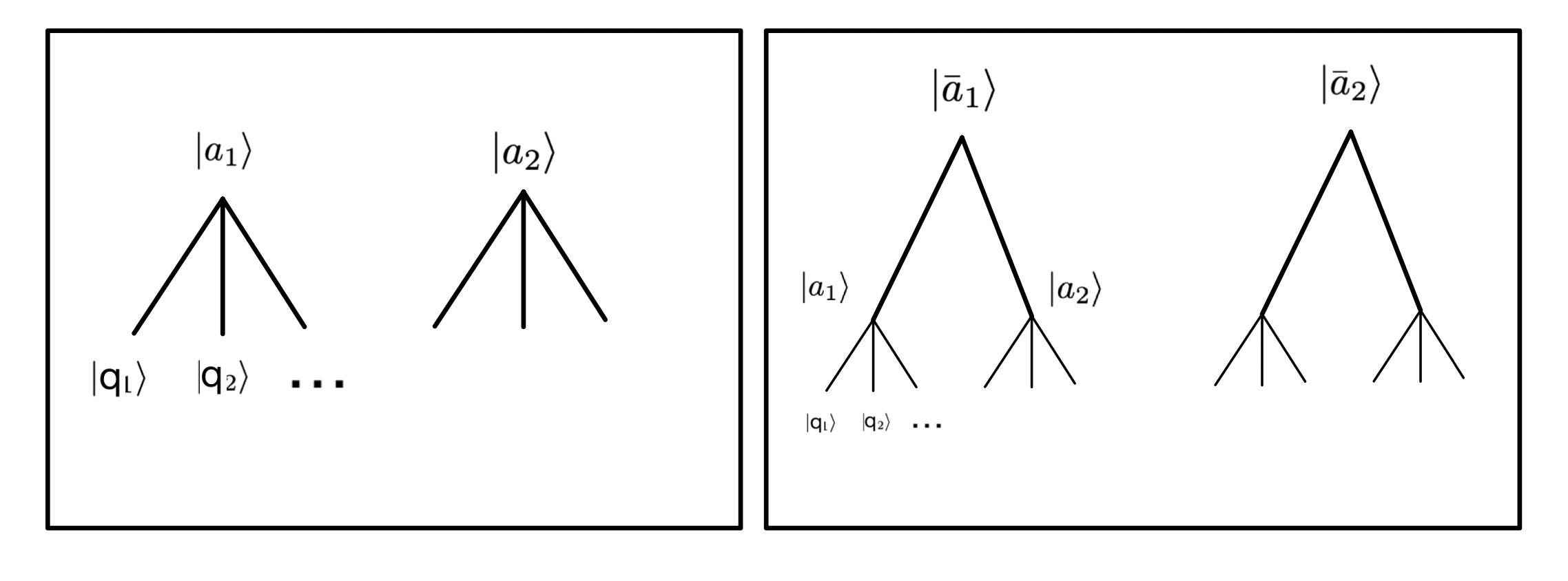
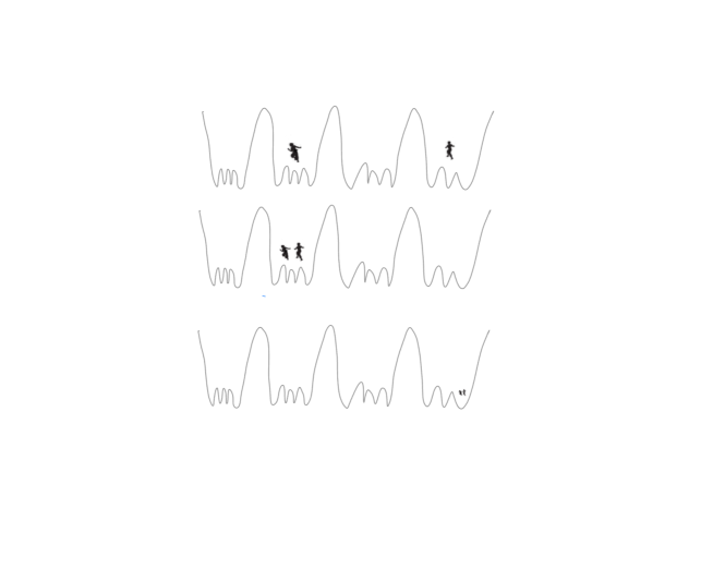
Figure 10: Hierarchical construction of states

10 Conclusions

If the connections pointed out in this paper turn out to be fruitful, the suggestion would be that glass physicists may be curious to take a deeper plunge in reparametrization and conformal questions, and those interested in toy gravity models, in replica theory and glassy dynamics.

References

- [1] H. Sompolinsky and A. Zippelius, Relaxational dynamics of the edwards-anderson model and the mean-field theory of spin-glasses, Phys. Rev. B 25, 6860 (Jun 1982).
- [2] L. F. Cugliandolo and J. Kurchan, Analytical solution of the off-equilibrium dynamics of a long-range spin-glass model, Physical Review Letters 71, 173 (7 1993).
- [3] L. F. Cugliandolo, J. Kurchan, P. Le Doussal and L. Peliti, Glassy behaviour in disordered systems with nonrelaxational dynamics, Physical review letters 78, p. 350 (1997).
- [4] H. E. Castillo, C. Chamon, L. F. Cugliandolo and M. P. Kennett, Heterogeneous aging in spin glasses, Phys. Rev. Lett. 88, p. 237201 (May 2002).
- [5] H. E. Castillo, C. Chamon, L. F. Cugliandolo, J. L. Iguain and M. P. Kennett, Spatially heterogeneous ages in glassy systems, Phys. Rev. B 68, p. 134442 (Oct 2003).
- [6] C. Chamon, M. P. Kennett, H. E. Castillo and L. F. Cugliandolo, Separation of time scales and reparametrization invariance for aging systems, Phys. Rev. Lett. 89, p. 217201 (Oct 2002).
- [7] C. Chamon and L. F. Cugliandolo, Fluctuations in glassy systems, J. Stat. Mech. 2007, p. P07022 (2007).
- [8] J. Kurchan, Time-reparametrization invariances, multithermalization and the parisi scheme, SciPost Physics Core 6, p. 001 (2023).
- [9] S. Sachdev and J. Ye, Gapless spin-fluid ground state in a random quantum Heisenberg magnet, Phys. Rev. Lett. 70, 3339 (May 1993).
- [10] A. Kitaev, A simple model of quantum holography, A simple model of quantum holography, http://online.kitp.ucsb.edu/online/entangled15/kitaev/, http://online.kitp.ucsb.edu/online/entangled15/kitaev2/, (2015).
- [11] O. Parcollet and A. Georges, Non-fermi-liquid regime of a doped mott insulator, Phys. Rev. B 59, 5341 (Feb 1999).
- [12] A. Georges, O. Parcollet and S. Sachdev, Mean field theory of a quantum Heisenberg spin glass, Phys. Rev. Lett. 85, 840 (Jul 2000).
- [13] A. Georges, O. Parcollet and S. Sachdev, Quantum fluctuations of a nearly critical Heisenberg spin glass, Phys. Rev. B 63, p. 134406 (Mar 2001).
- [14] J. Maldacena and D. Stanford, Remarks on the sachdev-ye-kitaev model, Phys. Rev. D 94, p. 106002 (Nov 2016).
- [15] J. Polchinski and V. Rosenhaus, The spectrum in the sachdev-ye-kitaev model, J. High Energy Phys. 2016, p. 1 (Apr 2016).
- [16] D. Facoetti, G. Biroli, J. Kurchan and D. R. Reichman, Classical glasses, black holes, and strange quantum liquids, Physical Review B 100, p. 205108 (2019).
- [17] A. Crisanti and H.-J. Sommers, The spherical p-spin interaction spin glass model: the statics, Z. Phys. B 87, 341 (Oct 1992).
- [18] A. Cavagna, Supercooled liquids for pedestrians, Physics Reports 476, 51 (2009).
- [19] T. Anous and F. M. Haehl, The quantum p-spin glass model: a user manual for holographers, Journal of Statistical Mechanics: Theory and Experiment 2021, p. 113101 (2021).
- [20] J. Cardy, Logarithmic conformal field theories as limits of ordinary cfts and some physical applications, Journal of Physics A: Mathematical and Theoretical 46, p. 494001 (2013).
- [21] L. F. Cugliandolo, J. Kurchan and L. Peliti, Energy flow, partial equilibration, and effective temperatures in systems with slow dynamics, Phys. Rev. E 55, 3898 (Apr 1997).
- [22] L. F. Cugliandolo and J. Kurchan, On the out-of-equilibrium relaxation of the sherrington-kirkpatrick model, Journal of Physics A: Mathematical and General 27, p. 5749 (1994).
- [23] T. Rizzo, Path integral approach unveils role of complex energy landscape for activated dynamics of glassy systems, Physical Review B 104, p. 094203 (2021).
- [24] A. Jevicki, K. Suzuki and J. Yoon, Bi-local holography in the syk model, Journal of High Energy Physics 2016, p. 7 (Jul 2016).
- [25] J. Zinn-Justin, Quantum Field Theory and Critical Phenomena (Oxford University Press, Oxford, 2002).
- [26] J. Kurchan, Six out of equilibrium lectures, Lecture Notes of the Les Houches Summer School, Vol. 90, Aug 2008 (Oxford University Press, Oxford, 2010), https://arxiv.org/abs/0901.1271arXiv:0901.1271.
- [27] B. Gaveau and L. S. Schulman, Theory of nonequilibrium first-order phase transitions for stochastic dynamics, J. Math. Phys. 39, 1517 (1998).
- [28] G. Biroli and J.-P. Bouchaud, Diverging length scale and upper critical dimension in the mode-coupling theory of the glass transition, Europhysics Letters (EPL) 67, 21 (jul 2004).
- [29] A. Bovier, M. Eckhoff, V. Gayrard and M. Klein, Metastability and low lying spectra¶in reversible markov chains, Commun. Math. Phys. 228, 219 (Jun 2002).
- [30] A. Biggs, J. Maldacena and V. Narovlansky, A supersymmetric syk model with a curious low energy behavior, arXiv preprint arXiv:2309.08818 (2023).
- [31] D. R. Reichman and P. Charbonneau, Mode-coupling theory, Journal of Statistical Mechanics: Theory and Experiment 2005, p. P05013 (2005).
- [32] W. Götze, Aspects of structural glass transitions, in Liquids, freezing and glass transition, Les Houches 1989 Les Houches 1989, (North-Holland, Amsterdam, 1991), Amsterdam.
- [33] W. Götze, Complex Dynamics of Glass-Forming Liquids (Oxford University Press, Oxford, 2008).
- [34] A. Crisanti and L. Leuzzi, Spherical 2+ p spin-glass model: An exactly solvable model for glass to spin-glass transition, Physical review letters 93, p. 217203 (2004).
- [35] W. Cottrell, B. Freivogel, D. M. Hofman and S. F. Lokhande, How to build the thermofield double state, Journal of High Energy Physics 2019, 1 (2019).
- [36] F. Pittorino, C. Lucibello, C. Feinauer, G. Perugini, C. Baldassi, E. Demyanenko and R. Zecchina, Entropic gradient descent algorithms and wide flat minima, Journal of Statistical Mechanics: Theory and Experiment 2021, p. 124015 (2021).
- [37] J. Kurchan, Supersymmetry in spin glass dynamics, J. Phys. I France 2, 1333 (1992).
- [38] S. Tănase-Nicola and J. Kurchan, Metastable states, transitions, basins and borders at finite temperatures, Journal of Statistical Physics 116, 1201 (2004).
- [39] E. Witten, Constraints on supersymmetry breaking, Nucl. Phys. B 202, 253 (1982).
- [40] D. Anninos, T. Anous and F. Denef, Disordered quivers and cold horizons, Journal of High Energy Physics 2016, 1 (2016).
- [41] J. Murugan, D. Stanford and E. Witten, More on supersymmetric and 2d analogs of the syk model, Journal of High Energy Physics 2017, 1 (2017).
- [42] J. Kent-Dobias and J. Kurchan, Complex complex landscapes, Physical Review Research 3, p. 023064 (2021).
- [43] A. J. Bray and M. A. Moore, Metastable states in spin glasses, Journal of Physics C: Solid State Physics 13, L469 (7 1980).
- [44] A. Cavagna, I. Giardina and G. Parisi, An investigation of the hidden structure of states in a mean-field spin-glass model, Journal of Physics A: Mathematical and General 30, 7021 (10 1997).
- [45] A. Cavagna, I. Giardina and G. Parisi, Structure of metastable states in spin glasses by means of a three replica potential, Journal of Physics A: Mathematical and General 30, 4449 (7 1997).
- [46] A. Cavagna, I. Giardina and G. Parisi, Stationary points of the Thouless-Anderson-Palmer free energy, Phys. Rev. B 57, 11251 (May 1998).
- [47] A. Cavagna, I. Giardina and G. Parisi, Stationary points of the thouless-anderson-palmer free energy, Physical Review B 57, 11251 (5 1998).
- [48] A. Cavagna, I. Giardina and G. Parisi, Cavity method for supersymmetry-breaking spin glasses, Physical Review B 71, p. 024422 (1 2005).
- [49] Y. V. Fyodorov, Complexity of random energy landscapes, glass transition, and absolute value of the spectral determinant of random matrices, Physical Review Letters 92, p. 240601 (6 2004).
- [50] Y. V. Fyodorov and I. Williams, Replica symmetry breaking condition exposed by random matrix calculation of landscape complexity, Journal of Statistical Physics 129, 1081 (9 2007).
- [51] V. Ros, G. Biroli and C. Cammarota, Complexity of energy barriers in mean-field glassy systems, EPL (Europhysics Letters) 126, p. 20003 (may 2019).
- [52] V. Ros, G. Biroli and C. Cammarota, Complexity of energy barriers in mean-field glassy systems, EPL (Europhysics Letters) 126, p. 20003 (5 2019).
- [53] A. Auffinger, G. Ben Arous and J. Černý, Random matrices and complexity of spin glasses, Communications on Pure and Applied Mathematics 66, 165 (9 2012).
- [54] A. Auffinger and G. Ben Arous, Complexity of random smooth functions on the high-dimensional sphere, The Annals of Probability 41, 4214 (11 2013).
- [55] G. Ben Arous, E. Subag and O. Zeitouni, Geometry and temperature chaos in mixed spherical spin glasses at low temperature: The perturbative regime, Communications on Pure and Applied Mathematics 73, 1732 (11 2019).
- [56] M. Kac, On the average number of real roots of a random algebraic equation, Bulletin of the American Mathematical Society 49, 314 (4 1943).
- [57] H. W. Lin, J. Maldacena, L. Rozenberg and J. Shan, Holography for people with no time, SciPost Physics 14, p. 150 (2023).
- [58] A. J. Bray and D. S. Dean, Statistics of critical points of Gaussian fields on large-dimensional spaces, Physical Review Letters 98, p. 150201 (4 2007).
- [59] J. Kent-Dobias and J. Kurchan, How to count in hierarchical landscapes: A full solution to mean-field complexity, Physical Review E 107, p. 064111 (2023).
- [60] M. Mézard, G. Parisi and M. A. Virasoro, Spin Glass Theory and Beyond (World Scientific, Singapore, 1987).
- [61] J. Murugan, D. Stanford and E. Witten, More on supersymmetric and 2d analogs of the syk model, J. High Energy Phys. 2017, p. 146 (Aug 2017).
- [62] M. Mézard, G. Parisi and M. A. Virasoro, Spin glass theory and beyond: An Introduction to the Replica Method and Its Applications (World Scientific Publishing Company, 1987).
- [63] P. Contucci, F. Corberi, J. Kurchan and E. Mingione, Stationarization and multithermalization in spin glasses, SciPost Physics 10, p. 113 (2021).