Euler-Heisenberg black hole surrounded by perfect fluid dark matter

Abstract

The Euler-Heisenberg black hole surrounded by perfect fluid dark matter is studied. In order to derive the metric, we elaborate on a method for generating the metric and its associated conditions. Based on the metric we derived, we investigate the optical properties, including the photon orbit and the image of the thin accretion disk with the Novikov-Thorne model, as well as the thermodynamics in anti-de Sitter spacetime. Our research illustrated the influence of quantum electrodynamics effect and dark matter on the photon trajectories, and revealed that the phenomena of Doppler shift and gravitational redshift will drastically affect the observed intensity of the accretion disk. In the realm of thermodynamics, we calculated the phase transition and criticality in extended phase space. The result showed that the effect of dark matter will distinctly determine the number of critical points for the black hole.

I Introduction

There are many novel subjects studied by physicists since Einstein established the theory of general relativity Einstein1 ; Einstein2 ; Einstein3 . A very attractive object should be black hole. Despite its amazing physical properties, the existence of black hole has been proved by the gravitational wave observed by Laser Interferometer Gravitation Wave Observatory (LIGO) wave and the picture of supermassive black hole in the center of M87 galaxy captured by Event Horizon Telescope (EHT) M87I ; M87II ; M87III ; M87IV ; M87V .

Recently, a new type of black hole, Euler-Heisenberg (E-H) black hole has been studied EHbH1 ; EHbh2 ; EHbh3 ; EHbh4 ; EHsolution ; QED_EH . This black hole is based on a new theory, the E-H theory, which takes quantum electrodynamics (QED) effect into account EHtheory . And it is widely known in physical community that dark matter could potentially explain the expanding universe. As an example of researches for dark matter, DM1 ; DM2 ; DM3 ; DM4 ; DM5 studied the properties of perfect fluid dark matter (PFDM), which has attracted more interests of scientists.

The optical properties and thermodynamics of black holes are two crucial topics in black hole physics. Due to the extremely strong gravity of black hole, the surrounding light is significantly bent, leading to fascinating optical phenomena, with the shadow and image of accretion disk being most captivating image1 ; image2 ; image3 ; shadow . In terms of thermodynamics, since Hawking and Page firstly studied the thermodynamics of black hole in anti-de Sitter (AdS) spacetime Hawking1 , there are many significant researches published RN-Ads1 ; RN-Ads2 ; Kastor ; Dolan . Generally speaking, the variation of cosmological constant in extended phase space will lead to more interesting results.

In this paper, we study E-H black hole surrounded by PFDM. To obtain the metric of black hole, we discussed the generation of metric and its corresponding conditions in mathematical way. Utilizing the metric, we calculated the photon orbit and image of thin accretion disk based on Novikov-Thorne (N-T) model. Furthermore, we studied the thermodynamics of E-H-AdS black hole surrounded by PFDM, including its thermodynamic functions, thermodynamic first law, equation of state and phase transition.

This article is organized as follows. In Sec. II, we make a discussion about the generation of new metric and give the mathematical deductions in detail. In Sec. III, we obtain the metric of E-H black hole surrounded by PFDM, which is described by four parameters: mass $M$, electric charge $Q$, QED effect parameter $a$ and PFDM parameter $\alpha$. In Sec. IV, we calculate the photon orbit and plot the image of thin accretion disk using N-T model. We showed how the parameters influence the photon propagation and the effect of Doppler shift and gravitational redshift. In Sec. V, we take E-H black hole surrounded by PFDM into AdS spacetime and research its thermodynamics in extended phase space. We analyze the thermodynamic first law, equation of state and phase transition of black hole, showing the influence of PFDM on the number of critical points. Finally, we give a conclusion and outlook in Sec. VI. To simplify the calculations, we use $G=c=k=\hbar=1$ in this paper.

II Generation of new metric

Consider a action written as

$$S=\int\sqrt{-g}d^{4}x\left({\frac{R}{16\pi}+\sum_{i}\mathcal{L}^{\left(i\right)}}\right),$$ (II.1)

where $R$ is scalar curvature, which describes the gravitational field, and $\mathcal{L}^{\left(i\right)}$ is Lagrangian, which represents $i^{\rm{th}}$ effect, like electromagnetic field, dark matter, etc. And we suppose that every $\mathcal{L}^{\left(i\right)}$ has its spherically symmetric solution.

By varying the Eq. (II.1) with the respect to the $g^{\mu\nu}$, one could get the gravitational field equation,

$$R_{\mu\nu}-\frac{1}{2}g_{\mu\nu}R=8\pi T_{\mu\nu},$$ (II.2)

where $g_{\mu\nu}$ is metric, $R_{\mu\nu}$ is Ricci tensor, $R$ is scalar curvature, and $T_{\mu\nu}$ is energy momentum tensor, which is calculated by varying the Lagrangian,

$$T_{\mu\alpha} =-\frac{2}{\sqrt{-g}}\frac{\partial\left(\sqrt{-g}\sum_{i}\mathcal{L}^{\left(i\right)}\right)}{\partial g^{\mu\alpha}}$$ (II.3)

$$=\sum_{i}-\frac{2}{\sqrt{-g}}\frac{\partial\left(\sqrt{-g}\mathcal{L}^{\left(i\right)}\right)}{\partial g^{\mu\alpha}}$$

$$=\sum_{i}T_{\mu\alpha}^{\left(i\right)},$$

where $g$ is determinant of $g_{\mu\nu}$.

Now consider a specific circumstance that Lagrangian $\mathcal{L}^{\left(i\right)}$ that describes different effects in Eq. (II.1) are independent.

Generally, the form of $\mathcal{L}^{\left(i\right)}$ should be

$$\mathcal{L}^{\left(i\right)}=\mathcal{L}^{\left(i\right)}\left(g^{\mu\nu},A_{\nu}^{\left(i\right)},\partial_{\mu}A_{\nu}^{\left(i\right)}\right),$$ (II.4)

where $A_{\mu}^{\left(i\right)}$ describes the $i^{\rm{th}}$ effect. For the mathematical simplicity, here we just consider the first derivative of $A_{\mu}^{\left(i\right)}$ and their linear terms. As an example, for electromagnetic field, it is four-potential we all know. The independence of $\mathcal{L}^{\left(i\right)}$ means that $\mathcal{L}^{\left(i\right)}$ should have no relationship with $A_{\mu}^{\left(j\right)}$, for $i\neq j$, and no relationship with $\partial_{\mu}A_{\nu}^{\left(j\right)}$ of course. In a word, this specific circumstance can be expressed as

$$\frac{\delta\mathcal{L}^{\left(i\right)}}{\delta A_{\mu}^{\left(j\right)}}=0,$$ (II.5)

for $i\neq j$.
Theoretically, if there are two effects coupled with each other, there should be a Lagrangian representing the interaction between them,

$$\mathcal{L}^{\left(i,j\right)}=\mathcal{L}^{\left(i,j\right)}\left(g^{\mu\nu},A_{\nu}^{\left(i\right)},A_{\nu}^{\left(j\right)},\partial_{\mu}A_{\nu}^{\left(i\right)},\partial_{\mu}A_{\nu}^{\left(j\right)}\right).$$ (II.6)

Only combining $\mathcal{L}^{\left(i,j\right)}$, $\mathcal{L}^{\left(i\right)}$ and $\mathcal{L}^{\left(j\right)}$ as one term could deal with this problem.

For simplicity of subsequent discussion, we use $g^{\mu\nu}$ to raise index of Eq. (II.2) and get following form of field equation,

$$R_{\mu}^{\nu}-\frac{1}{2}\delta_{\mu}^{\nu}R=8\pi\sum_{i}T_{\mu}^{\nu\left(i\right)},$$ (II.7)

where $T_{\mu}^{\nu\left(i\right)}=g^{\nu\alpha}T_{\mu\alpha}^{\left(i\right)}$. We require that the energy momentum tensor $T_{0}^{{0}\left(i\right)}$ is independent from spacetime itself for the case of spherically symmetric spacetime.

Let’s make it clear, it means after solving the field equation of $A_{\mu}^{\left(i\right)}$ with some specific physical backgrounds,

$$\frac{\delta}{\delta A_{\mu}^{\left(i\right)}}\int\sqrt{-g}d^{4}x\mathcal{L}^{\left(i\right)}=0,$$ (II.8)

and substituting the solution and spherically symmetric metric when only $\mathcal{L}^{\left(i\right)}$ exists,

$$g_{\mu\nu}=g_{\mu\nu}^{\left(i\right)}=diag\left(-\left(1+f_{i}\left(r\right)\right),\frac{1}{1+f_{i}\left(r\right)},r^{2},r^{2}\sin{\theta}\right)$$ (II.9)

into $T_{0}^{0\left(i\right)}$, the result should be independent from the function $f_{i}\left(r\right)$ and its derivatives.
Using mathematical word could make it clear to understand. We assume $A_{\mu}^{0\left(i\right)}$ is the solution of Eq. (II.8), we should have

$$\frac{\delta}{\delta f_{i}\left(r\right)}\left(T_{0}^{0\left(i\right)}\Bigg{|}_{A_{\mu}^{\left(i\right)}=A_{\mu}^{0\left(i\right)},g_{\mu\nu}=g_{\mu\nu}^{\left(i\right)}}\right)=0.$$ (II.10)

We can further calculate Eq. (II.10) and get

$$\frac{\delta}{\delta f_{i}\left(r\right)}\left\{\left(\frac{1}{2}\mathcal{L}^{\left(i\right)}+\frac{1}{1+f_{i}\left(r\right)}\frac{\partial\mathcal{L}^{\left(i\right)}}{\partial g^{00}}\right)\Bigg{|}_{A_{\mu}^{\left(i\right)}=A_{\mu}^{0\left(i\right)},g_{\mu\nu}=g_{\mu\nu}^{\left(i\right)}}\right\}=0.$$ (II.11)

Now we try to get the spherically symmetric solution of Eq. (II.7) under above two requirements.

One could get $A_{\mu}^{\left(j\right)}$ from

$$\frac{\delta}{\delta A_{\mu}^{\left(j\right)}}\int\sqrt{-g}d^{4}x\sum_{i}\mathcal{L}^{\left(i\right)}=0.$$ (II.12)

According to independence of $\mathcal{L}^{\left(i\right)}$, this equation is equivalent to Eq. (II.8). We assume $A_{\mu}^{0\left(i\right)}$ is the solution of Eq. (II.8).
Assume the solution of Eq. (II.7) is

$$g_{\mu\nu}=g_{\mu\nu}^{\left(0\right)}=diag\left(-\left(1+f\left(r\right)\right),\frac{1}{1+f\left(r\right)},r^{2},r^{2}\sin{\theta}\right).$$ (II.13)

Substitute this solution into Eq. (II.7), we get nonzero terms,

$$\frac{f\left(r\right)+rf^{\prime}\left(r\right)}{r^{2}}=8\pi\sum_{i}T_{0}^{0\left(i\right)}\Bigg{|}_{A_{\mu}^{\left(i\right)}=A_{\mu}^{0\left(i\right)},g_{\mu\nu}=g_{\mu\nu}^{\left(0\right)}}.$$ (II.14)

Substitute Eq. (II.9) into the field equation that only $\mathcal{L}^{\left(i\right)}$ works, we get nonzero terms,

$$\frac{f_{i}\left(r\right)+rf_{i}^{\prime}\left(r\right)}{r^{2}}=8\pi T_{0}^{0\left(i\right)}\Bigg{|}_{A_{\mu}^{\left(i\right)}=A_{\mu}^{0\left(i\right)},g_{\mu\nu}=g_{\mu\nu}^{\left(i\right)}}.$$ (II.15)

Use Eq. (II.11), we can surely replace $g_{\mu\nu}^{\left(i\right)}$ in Eq. (II.15) with $g_{\mu\nu}^{\left(0\right)}$. Furthermore, we combine Eq. (II.14) and Eq. (II.15) and get

$$f\left(r\right)+rf^{\prime}\left(r\right)=\sum_{i}\left(f_{i}\left(r\right)+rf_{i}^{\prime}\left(r\right)\right),$$ (II.16)

whose general solution is

$$f\left(r\right)=\frac{C}{r}+\sum_{i}f_{i}\left(r\right),$$ (II.17)

where $C$ is integration constant to be determined.

So we finally get the solution of Eq. (II.7),

$$ds^{2}=-\left(1+f\left(r\right)\right)dt^{2}+ \frac{1}{1+f\left(r\right)}dr^{2}+r^{2}d\Omega^{2},$$ (II.18)

$$f\left(r\right)=\frac{C}{r}+ \sum_{i}f_{i}\left(r\right),$$

Now, it’s necessary to point out that above discussion is just a mechanical deduction. In practice, if we could replace $T_{0}^{0\left(i\right)}$ in case of various interactions with $T_{0}^{0\left(i\right)}$ when there is only one interaction, in other word, if spacetime itself has no influence on the form of $T_{0}^{0\left(i\right)}$, then we can draw a conclusion that the metric function will meet with simple formula as Eq. (II.17). Just in a mathematical way, Eq. (II.5) and Eq. (II.10) we have required in previous content can insure this circumstance indeed.

We can propose $f_{i}\left(r\right)$ in Eq. (II.9) as a influence the interaction $\mathcal{L}^{\left(i\right)}$ exerts on the flat spacetime. So, if many interactions have no influences on each other, this impact on the spacetime can get simply superimposed mathematically. Moreover, Schwawrzschild-like term $C/r$ in Eq. (II.17) will not hinder the superimposition of impacts of multiple interactions because $C/r$ has no contribution to energy momentum tensor. Constant $C$ should be decided by some rational physical meanings.

III E-H Black Hole surrounded by PFDM

In this section, we will use the method in the previous section to construct a spherically symmetric spacetime, which describe a E-H black hole surrounded by PFDM. The optical properties and thermodynamics will be investigated in Sec. IV and Sec. V.

Firstly, EHsolution ; QED_EH provides the metric of E-H black hole,

$$ds^{2}=-\left(1+f_{1}\left(r\right)\right)dt^{2} +\frac{1}{1+f_{1}\left(r\right)}dr^{2}+r^{2}d\Omega^{2},$$ (III.1)

$$f_{1}\left(r\right)=-\frac{2M}{r} +\frac{Q^{2}}{r^{2}}-\frac{aQ^{4}}{20r^{6}},$$

its corresponding energy momentum tensor can be found from EHbH1 ,

$$T_{t}^{t}=T_{r}^{r}=\frac{1}{4\pi}\left(-\frac{Q^{2}}{2r^{4}}+\frac{aQ^{4}}{8r^{8}}\right),$$ (III.2)

$$T_{\theta}^{\theta}=T_{\phi}^{\phi}=\frac{1}{4\pi}\left(\frac{Q^{2}}{2r^{4}}-\frac{3aQ^{4}}{8r^{8}}\right),$$

where $M$ is the mass of the black hole, $Q$ is the electric charge of the black hole and $a$ is the QED parameter which is used to measure the strength of the QED correction.

Secondly, we use the energy momentum tensor of PFDM mentioned in ZhangHexuBardeen ,

$$T_{t}^{t}=T_{r}^{r}=\frac{\alpha}{8\pi r^{3}},$$ (III.3)

$$T_{\theta}^{\theta}=T_{\phi}^{\phi}=-\frac{\alpha}{16\pi r^{3}},$$

where $\alpha$ is the dark matter parameter.
Via substituting Eq. (III.3) into Eq. (II.14), one can easily get the metric of PFDM,

$$ds^{2}=-\left(1+f_{2}\left(r\right)\right) dt^{2}+\frac{1}{1+f_{2}\left(r\right)}dr^{2}+r^{2}d\Omega^{2},$$ (III.4)

$$f_{2}\left(r\right) =\frac{\alpha}{r}\ln{\frac{r}{\left|\alpha\right|}}.$$

Considering that dark matter won’t participate with the electromagnetic interaction and it is obvious that above two energy momentum tensors are both independent from metric function $f\left(r\right)$ to be determined. According to generation method we studied in Sec. II, we got the metric of E-H black hole surrounded by PFDM,

$$g_{\mu\nu} =diag\left(-g\left(r\right),\frac{1}{g\left(r\right)},r^{2},r^{2}\sin^{2}\left(\theta\right)\right),$$ (III.5)

$$g\left(r\right) =1-\frac{2M}{r}+\frac{Q^{2}}{r^{2}}-\frac{aQ^{4}}{20r^{6}}+\frac{\alpha}{r}\ln\left(\frac{r}{\left|\alpha\right|}\right).$$

Please notice that we have chosen integration constant $C$ as zero to insure that Eq. (III.5) can degenerate to E-H black hole by choosing PFDM parameter $\alpha$ as zero.

It’s easy to see that parameter $\alpha$ describes the strength of dark matter, and parameter $a$ describes the QED effect. Particularly, when $\alpha=0$, it goes back to the E-H black hole; when $a=0$, QED effect vanishes and RN black hole surrounded by PFDM appears; if $\alpha=0$ and $a=0$, we get simple RN black hole.

For the convenience of calculation, we will uniformly use $M=1$ in the subsequent figure presentations.

IV Optical properties

In this section, we will study the optical properties of E-H black hole surrounded by PFDM, including the photon orbit and image of a thin accretion disk.

IV.1 Geodesic equation and photon orbit

Let’s consider a particle moving in a spherically symmetric spacetime,

$$ds^{2}=-g\left(r\right)dt^{2}+\frac{dr^{2}}{g\left(r\right)}+r^{2}d\Omega^{2}$$ (IV.1)

where $d\Omega^{2}=d\theta^{2}+\sin^{2}{\theta}d\phi^{2}$ is Euclidean line element on two-dimensional sphere.
Lagrangian of a particle is

$$\mathcal{L}=\frac{1}{2}g_{\mu\nu}\dot{x}^{\mu}\dot{x}^{\nu},$$ (IV.2)

where $g_{\mu\nu}$ is metric, $\dot{x}^{\mu}=dx^{\mu}/d\lambda$ is four-velocity of particle, $\lambda$ is proper time $\tau$ for physical particle and affine parameter for photon. For simplicity of following calculation, we choose a appropriate coordinate system to ensure $\theta=\pi/2$, $\dot{\theta}=0$, which is to say particle moves in equatorial plane. Euler-Lagrange equation gives two conserved quantities,

$$E=-\frac{\partial\mathcal{L}}{\partial\dot{t}}=-g_{tt}\dot{t},$$ (IV.3)

$$L=\frac{\partial\mathcal{L}}{\partial\dot{\phi}}=g_{\phi\phi}\dot{\phi},$$ (IV.4)

where $E$ and $L$ represent the energy and angular momentum of particle. Eq. (IV.3) and Eq. (IV.4) are

$$\dot{t}=\frac{E}{g\left(r\right)},$$ (IV.5)

$$\dot{\phi}=\frac{L}{r^{2}}.$$ (IV.6)

According to Eq. (IV.2), Eq. (IV.5) and Eq. (IV.6), we have

$$\dot{r}^{2}=E^{2}-g\left(r\right)\frac{L^{2}}{r^{2}}+2g\left(r\right)\mathcal{L}.$$ (IV.7)

We use Eq. (IV.6) and Eq. (IV.7) to eliminate parameter $\lambda$,

$$\left(\frac{dr}{d\phi}\right)^{2}=r^{4}\left(\frac{1}{b^{2}}-\frac{g\left(r\right)}{r^{2}}+\frac{2g\left(r\right)\mathcal{L}}{L^{2}}\right)=:V_{eff},$$ (IV.8)

where $b=L/E$ is impact parameter. Here we have introduced a new function $V_{eff}$ we called ‘effective potential’.

Now we consider the motion of photon. For photon, $\mathcal{L}=0$, Eq. (IV.8) becomes

$$\left(\frac{dr}{d\phi}\right)^{2}=r^{4}\left(\frac{1}{b^{2}}-\frac{g\left(r\right)}{r^{2}}\right).$$ (IV.9)

We make a transform $u=1/r$ to rewrite Eq. (IV.9) as

$$\left(\frac{du}{d\phi}\right)^{2}=G\left(u\right),$$ (IV.10)

where

$$G\left(u,b\right)=\frac{1}{b^{2}}-u^{2}\left(1-2Mu+Q^{2}u^{2}-\frac{aQ^{4}}{20}u^{6}-u\alpha\ln\left(u\left|\alpha\right|\right)\right).$$ (IV.11)

For photon, parameter $b$ has a very visualized physical meaning. It is the distance from the black hole to the asymptotic line of photon orbit at infinity.

We first focus on the circular orbit of photon, which satisfies $V_{eff}=V_{eff}^{\prime}=0$. We record the solution as $r=r_{ph}$ and $b=b_{c}$. $r_{ph}$ is the radius of circular orbit. Please notice that we record $dA/dr=A^{\prime}$ for any scalar function $A$.
Next, we will see how the value of $b$ influences the light’s motion form infinity. For this, We take $M=Q=a=1,\alpha=-0.5$ for an example and plot the function $V_{eff}\left(r\right)$ for different $b$ in Fig. IV.1.

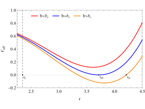
Figure IV.1: Variation of $V_{eff}$ with respect to $r$. The red, blue and orange lines represent $b<b_{c}$, $b=b_{c}$ and $b>b_{c}$ respectively. The black dashed line represents event horizon. $r_{h}$ is radius of horizon, $r_{ph}$ is radius of circular orbit and $r_{m}$ is the maximum positive root of the curve $V_{eff}$ for $b>b_{c}$. We set $Q=a=1,\alpha=-0.5$.

As we can see in Fig. IV.1:
For $b>b_{c}$, there is a maximum positive root $r_{m}\left(b\right)$ of $V_{eff}$. The photon comes from infinity and will never enter the region $r<r_{m}$. Instead, it will reach the point $r_{m}$ and then return to infinity along a path with the same shape as the incoming trajectory; For $b=b_{c}$, the photon will arrive $r=r_{ph}$ and then perpetually undergo circular motion; For $b<b_{c}$, the photon will continuously approach the black hole until they fall into the horizon $r=r_{h}$.
Here we define a function $\Phi_{b}\left(r\right)=\int_{0}^{\frac{1}{r}}\frac{1}{\sqrt{G\left(u,b\right)}}\,du$, then Eq. (IV.10) gives the total change of azimuth angle $\varphi$ for a certain orbit with the respect to $b$,

$$\varphi\left(b\right)=\begin{cases}\Phi_{b}\left(r_{h}\right),&b<b_{c},\\ 2\Phi_{b}\left(r_{m}\right),&b>b_{c}.\end{cases}$$ (IV.12)

Obviously there is $\lim_{b\to\ b_{c}}\varphi\left(b\right)=+\infty$.
Here we give the graph of $\phi\left(b\right)$ and photon orbits diagram in Fig. IV.2.

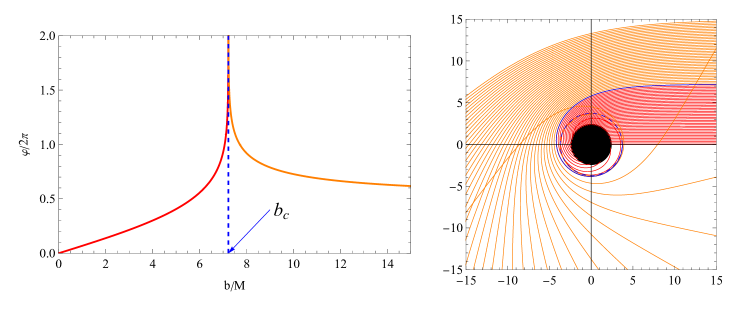
Figure IV.2: (a) Graph of function $\varphi\left(b\right)$. (b) Photon orbits for different values of $b$. The red curves, blue curve and orange curves correspond to $b<b_{c}$, $b=b_{c}$ and $b>b_{c}$. The black hole is represented by the central black region in (b). We set $Q=a=1,\alpha=-0.5$.

We can clearly see that figure agrees with our analysis.
And we can go further to investigate how parameters $Q$, $a$ and $\alpha$ influence the motion of photon.

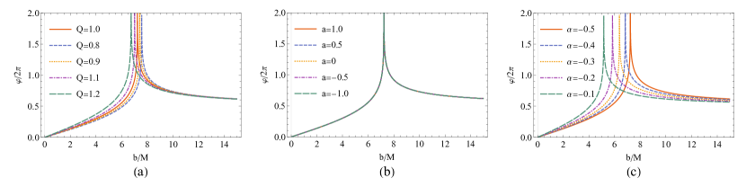
Figure IV.3: Graphs of $\varphi\left(b\right)$ for different parameters $Q$, $a$ and $\alpha$. We set (a) $a=0$, $\alpha=-0.5$, (b) $Q=1$, $\alpha=-0.5$, (c) $Q=1$, $a=1$.

Fig. IV.3 gives $\varphi\left(b\right)$ for different parameters. It shows $b_{c}$ will decrease with the increase of magnitude of $\alpha$ and $Q$. And QED effect has almost no impact on the photon’s orbit. We notice that the results showed the effects of $Q$ and $a$ agree with QED_EH , so we will only pay attention to the influence of PFDM on the image of thin accretion disk in next subsection.

IV.2 Image of thin accretion disk

In this section, we investigate the image of thin accretion disk.

Due to black hole’s strong gravity, even light cannot escape, so black hole itself can’t be observed by optical instrument. But generally, there is a accretion disk around the black hole. Because of the high-speed rotation of matter on the accretion disk, the effects of friction, collisions, and compression will result in intense thermal radiation, which can be observed by external observers.

‘Thin accretion disk’ means that we abstract the accretion disk into a plane with negligible thickness, and we ignore the influence of accretion disk on the black hole’s spacetime.

We assume the observer is at infinity to ensure that the light rays are approximately parallel rays, which will simplify our discussion. We give the coordinate system as Fig. IV.4.

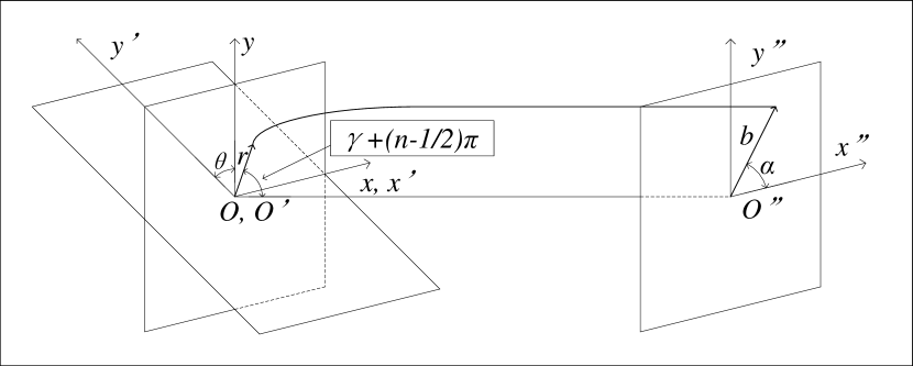
Figure IV.4: Coordinate system.

The center of black hole is located at point $O,O^{\prime}$. Accretion disk is in the $x^{\prime}O^{\prime}y^{\prime}$ plane, observer is on $x^{\prime\prime}O^{\prime\prime}y^{\prime\prime}$ plane, which is used to show the image of disk. $xOy$ plane is parallel to $x^{\prime\prime}O^{\prime\prime}y^{\prime\prime}$ plane. The angle between $xOy$ plane and $x^{\prime}O^{\prime}y^{\prime}$ plane is $\theta$. We always build the right-handed Cartesian coordinate system based on the plane system we have chosen to finish the calculation.

Now let’s consider a photon, which is located at point $\left(b,\alpha\right)$ on $x^{\prime\prime}O^{\prime\prime}y^{\prime\prime}$ plane, departing in the vertical direction. The photon pass through the disk for $n$ times and finally arrive a point on the disk. And the distance from this point to the point $O,O^{\prime}$ is $r$. We assume the change of photon’s azimuth angle is $\gamma+\left(n-1/2\right)\pi$.
According to space analytic geometry, we have

$$\tan{\gamma}=\tan{\theta}\sin{\alpha}.$$ (IV.13)

And one can calculate the value of $r$ via photon’s geodesic equation, which has been discussed in detail in Sec. IV.2.
So now, if we fix $\theta$ and $n$, we will obtain a function,

$$r=r\left(b,\alpha\right).$$ (IV.14)

If we fix $r$, we will acquire a curve expressed by polar equation $b=b\left(\alpha\right)$ in $xOy$ plane. This curve is precisely the image of circular orbit with a radius of $r$ on the accretion disk. Because the photon in this case will pass through the accretion disk for $n$ times, we call this image ‘$n^{\rm{th}}$ order image’.

Now we introduce a crucial concept: the inner edge $r_{in}$ of accretion disk. The inner edge $r_{in}$ of the accretion disk actually means the innermost stable circular orbit, because circular orbits within this range will be unstable, such that the particle will fall into or escape from the black hole when it is perturbed. $r_{in}$ satisfies

$$V_{eff}=V_{eff}^{\prime}=V_{eff}^{\prime\prime}=0.$$ (IV.15)

Before we plot the image of accretion disk, it’s worth mentioning that according to analysis in image1 , when $n\geq 3$, $n^{\rm{th}}$ order image is negligible. So we plot the first and second order images of accretion disk for different azimuth angles $\theta$ of observer.

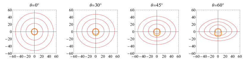
Figure IV.5: The first order images (red lines) and second order images (orange lines) of circular orbit $r=\rm{constant.}$ on accretion disk. The values of $r$ are chosen from $r_{in}$ to $50M$ equidistantly. $\theta$ from left to right are $0$, $\pi/6$, $\pi/4$ and $\pi/3$ respectively. We set $Q=a=1$, $\alpha=-0.5$.

As we can see in Fig. IV.5, when the observer observes from the North Pole direction of black hole, a series of circles will appear, which is consistent with the symmetry of spacetime. And as $\theta$ increases, the first order image gradually takes on a hat-like shape. It indicate that the azimuth of observer has a significant impact on the obtained results.

To obtain the image with brightness. We use the Novikov-Thorne model of radiation flux of accretion disk proposed in radiation_flux1 ; radiation_flux2 ,

$$F\left(r\right)=-\frac{\mathcal{M}\Omega^{\prime}}{4\pi\sqrt{-g}\left(E-\Omega L\right)^{2}}\int_{r_{in}}^{r}\left(E-\Omega L\right)L^{\prime}dr,$$ (IV.16)

where $\mathcal{M}$ is black hole’s accretion rate, $g$ is the metric determinant, and $r_{in}$ represents the inner edge of the accretion disk. $E$, $\Omega$, and $L$ are the energy, angular velocity, and angular momentum of physical particles moving on the accretion disk.
For further analysis, we need to calculate the motion of physical particles. We set accretion disk in the equatorial plane and consider a particle moving in a circular orbit around the black hole on the disk. For physical particles, $\mathcal{L}=-1/2$, that is

$$g_{tt}\dot{t}^{2}+g_{\phi\phi}\dot{\phi}^{2}=-1.$$ (IV.17)

We take the derivative of $r$ for both sides,

$$g_{tt}^{\prime}\dot{t}^{2}+g_{\phi\phi}^{\prime}\dot{\phi}^{2}=0.$$ (IV.18)

So we obtain the angular velocity $\Omega$ of particle,

$$\Omega=\frac{d\phi}{dt}=\pm\sqrt{\frac{g_{tt}^{\prime}}{g_{\phi\phi}^{\prime}}}.$$ (IV.19)

Plus and minus signs indicate two different directions of rotation and they have no essential distinction. We take plus sign in future calculations. Energy and angular momentum are given by Eq. (IV.3) and Eq. (IV.4):

$$E=\frac{-g_{tt}}{\sqrt{g_{tt}-g_{\phi\phi}\Omega^{2}}},$$ (IV.20)

$$L=\frac{g_{\phi\phi}\Omega}{\sqrt{g_{tt}-g_{\phi\phi}\Omega^{2}}}.$$ (IV.21)

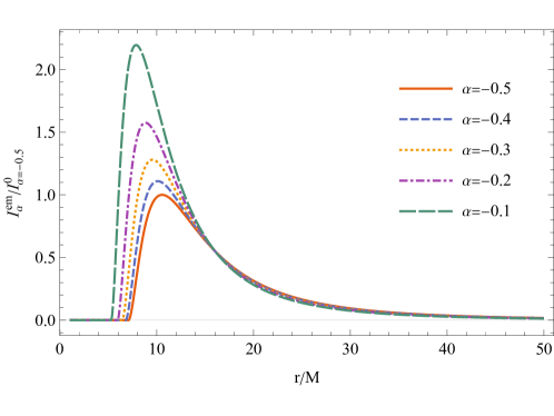
Figure IV.6: Graphs of relative radiation flux for different $\alpha$. $I_{\alpha}^{em}$ is the radiation flux $F\left(r\right)$. $I_{\alpha=-0.5}^{0}$ is the maximum value of radiation flux for $\alpha=-0.5$. We set $Q=a=1$.

We are particularly interested in the influence of PFDM. Fig. IV.6 shows how PFDM affects the radiation flux of accretion disk. At short distances, the dark matter effect will significantly diminish the radiation flux. In contrast, at greater distances, the radiation flux will increase with the growth of $\alpha$.
Due to the different gravitational fields at disk and observer, as well as their relative motion, there will be frequency shift phenomenon. According to image1 , the radiation flux observer received will be

$$F_{obs}=\frac{F\left(r\right)}{\left(1+z\right)^{4}},$$ (IV.22)

where $z$ is redshift factor, which is defined by

$$1+z=\frac{E_{em}}{E_{obs}},$$ (IV.23)

$E_{em}$ and $E_{obs}$ are the the emitted light intensity at the light source and the light intensity received by the observer, respectively.
According to image2 , $E_{em}$ can be expressed as

$$E_{em}=-p_{\mu}u^{\mu},$$ (IV.24)

where $p_{\mu}=g_{\mu\nu}\dot{x^{\nu}}$ is photon’s four-momentum and $u^{\mu}$ is particle’s four-velocity. And energy observer received at infinity is naturally $E=-p_{t}$. So,

$$1+z=\frac{p_{t}u^{t}+p_{\phi}u^{\phi}}{p_{t}}=u^{t}\left(1+\Omega\frac{p_{\phi}}{p_{t}}\right),$$ (IV.25)

Please notice that our tensor calculations are performed in $x^{\prime}O^{\prime}y^{\prime}$ coordinate system, which take accretion disk as its equatorial plane. According to the coordinate transform between system $x^{\prime}O^{\prime}y^{\prime}$ and system $O^{\prime\prime}O^{\prime}\vec{r}$, whose equatorial plane is the photon’s propagation plane, we can prove

$$\left(\frac{p_{\phi}}{p_{t}}\right)_{x^{\prime}O^{\prime}y^{\prime}}=\sin\theta\cos\alpha\left(\frac{p_{\phi}}{p_{t}}\right)_{O^{\prime\prime}O^{\prime}\vec{r}},$$ (IV.26)

and due to the light is emitted from the accretion disk to infinity, compared to our previous formula, there will be an additional negative sign to the value of $p_{\phi}$, that is to say $\left(p_{\phi}\right)_{O^{\prime\prime}O^{\prime}\vec{r}}=-L$. So we finally get

$$\left(\frac{p_{\phi}}{p_{t}}\right)_{O^{\prime\prime}O^{\prime}\vec{r}}=\frac{L}{E}=b,$$ (IV.27)

where $b$ is precisely impact parameter shown in Fig. IV.4. Thus,

$$1+z=\frac{1+b\sin\theta\cos\alpha}{\sqrt{-g_{tt}-g_{\phi\phi}\Omega^{2}}}.$$ (IV.28)

Utilizing above analysis, now we can plot the image of the accretion disk with intensity distribution.

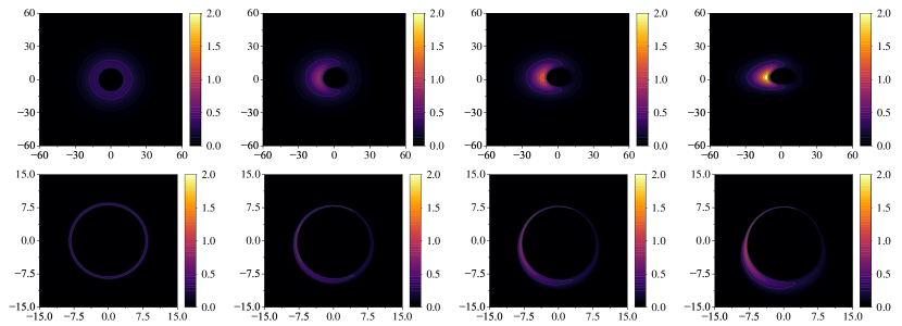
Figure IV.7: First and second order images of accretion disk for different $\theta$. $\theta$ from left to right are $0$, $\pi/6$, $\pi/4$ and $\pi/3$ respectively. We set $Q=a=1$, $\alpha=-0.5$.

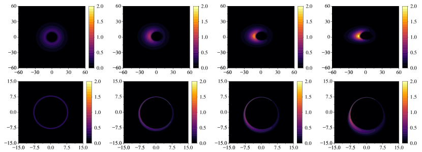
Figure IV.8: First and second order images of accretion disk for different $\theta$. $\theta$ from left to right are $0$, $\pi/6$, $\pi/4$ and $\pi/3$ respectively. We set $Q=a=1$, $\alpha=-0.4$.

We plot the first and second order images with relative intensity distribution of thin accretion disk for different values of $\alpha$ and $\theta$ in Fig. IV.7 and Fig. IV.8.
The figures clearly show:
(i) The results basically accord with the images in Fig. IV.5;
(ii) Compare to the first order image, the second order image already became very weak. It’s foreseeable that for $n\geq 3$, the image will be negligible;
(iii) Doppler frequency shift effect is very evident. It cause the brightness on the left side of the accretion disk is noticeably stronger than right side’s, because the matter on the left side of disk moves toward the observer;
(iv) The brightness of disk when $\alpha=-0.4$ is more strong than the case $\alpha=-0.5$. This phenomenon generally conforms to the result in Fig. IV.6, showing that the more intense dark matter effects will significantly reduce the brightness of disk. Although at a long distance, PFDM will increase the radiation flux lowly, the radiation flux rapidly tends to zero, making it appear negligible in image of accretion disk.

V Thermodynamics

In this section, we will investigate the thermodynamics of E-H black hole surrounded by PFDM in AdS spacetime. Research for black hole thermodynamics in extended phase space requires us to regard cosmological constant $\Lambda$ as a thermodynamic variable. It seems to have contradiction, but there are also some good reasons why the variation of $\Lambda$ should be included in thermodynamic considerations criticalexponent1 . And it’s clear to see the physical meaning in Kastor , which shows that $\Lambda$ is regarded as pressure,

$$P=-\frac{\Lambda}{8\pi}.$$ (V.1)

V.1 E-H-AdS black hole surrounded by PFDM

We can regard the cosmological constant $\Lambda$ as an effect of special Lagrangian written as

$$\mathcal{L}^{\left(\Lambda\right)}=-\frac{\Lambda}{8\pi}.$$ (V.2)

The energy momentum tensor generated from $\mathcal{L}_{\Lambda}$ is

$$T_{\mu\nu}^{\left(\Lambda\right)}=-\frac{2}{\sqrt{-g}}\frac{\partial\sqrt{-g}\mathcal{L}^{\left(\Lambda\right)}}{\partial{g^{\mu\nu}}}=-\frac{\Lambda g_{\mu\nu}}{8\pi},$$ (V.3)

which caused field equation with cosmological constant.
Anti-de Sitter spacetime is

$$ds^{2}_{AdS}=-\frac{1}{\left(1-\frac{\Lambda r^{2}}{3}\right)}dt^{2}+\left(1-\frac{\Lambda r^{2}}{3}\right)dr^{2}+r^{2}d\Omega^{2}.$$ (V.4)

Its energy momentum tensor

$$T_{0}^{0\left(\Lambda\right)}=g^{0\alpha}T_{0\alpha}^{\left(\Lambda\right)}=-\frac{\Lambda}{8\pi},$$ (V.5)

which apparently is just a constant without $f\left(r\right)$. And further, E-H theory and model of PFDM have nothing to do with cosmological constant itself. That is to say, these three effects have no interaction.

According to the metric generation method we discussed in Sec. II, when we take the E-H black hole surrounded by PFDM into AdS spacetime, the metric will convert to

$$g_{\mu\nu}=diag\left(-g\left(r\right),\frac{1}{g\left(r\right)},r^{2},r^{2}\sin^{2}\left(\theta\right)\right),$$ (V.6)

$$g\left(r\right) =1-\frac{2M}{r}+\frac{Q^{2}}{r^{2}}-\frac{aQ^{4}}{20r^{6}}+\frac{\alpha}{r}\ln\left(\frac{r}{\left|\alpha\right|}\right)-\frac{\Lambda r^{2}}{3}.$$

V.2 Thermodynamic functions and equation of state

The mass of the black hole is solved from $g\left(r_{h}\right)=0$,

$$M=\frac{r_{h}}{2}\left(1+\frac{\alpha}{r_{h}}\ln\left(\frac{r_{h}}{\left|\alpha\right|}\right)-\frac{\Lambda r_{h}^{2}}{3}+\frac{Q^{2}}{r_{h}^{2}}-\frac{aQ^{4}}{20r_{h}^{6}}\right).$$ (V.7)

The Hawking temperature of the black hole is defined by its surface gravity TH ,

$$T_{H}=\frac{g^{\prime}\left(r_{h}\right)}{4\pi}=\frac{1}{4\pi r_{h}}\left(1-\frac{Q^{2}}{r_{h}^{2}}+\frac{aQ^{4}}{4r_{h}^{6}}-\Lambda r_{h}^{2}+\frac{\alpha}{r_{h}}\right).$$ (V.8)

The corresponding black hole entropy is

$$S=\pi r_{h}^{2}.$$ (V.9)

Thermodynamic first law is

$$dM=TdS+VdP+\Phi dQ+\mu d\alpha.$$ (V.10)

Here M is mass of black hole, which is also interpreted as enthalpy. $T$ is temperature, $V$ is thermodynamic volume of black hole, $\Phi$ is electric potential and $\mu$ can be treated as dark matter potential. Thermodynamic functions $V$, $\Phi$ and $\mu$ can be calculated form Eq. (V.10),

$$V=\left(\frac{\partial M}{\partial P}\right)_{S,Q,\alpha}=\frac{4\pi r_{h}^{3}}{3}.$$ (V.11)

$$\Phi=\left(\frac{\partial M}{\partial Q}\right)_{S,P,\alpha}=\frac{Q}{r_{h}}-\frac{aQ^{3}}{10r_{h}^{5}}.$$ (V.12)

$$\mu=\left(\frac{\partial M}{\partial\alpha}\right)_{S,P,Q}=\frac{1}{2}\left(\ln{\frac{r_{h}}{\left|\alpha\right|}}-1\right).$$ (V.13)

Now it’s crucial to verify whether $T=T_{H}$ because $T\neq T_{H}$ is actually possible criticalexponent2 . If $T\neq T_{H}$, revising thermodynamic first law becomes necessary.
For our black hole,

$$T=\left(\frac{\partial M}{\partial S}\right)_{P,Q,\alpha}.$$ (V.14)

For any $A$, one can obtain

$$\frac{\partial A}{\partial S}=\frac{1}{2\pi r_{h}}\frac{\partial A}{\partial r_{h}}.$$ (V.15)

So we have

$$T=\frac{M^{\prime}\left(r_{h}\right)}{2\pi r_{h}}=\frac{1}{4\pi r_{h}}\left(1-\frac{Q^{2}}{r_{h}^{2}}+\frac{aQ^{4}}{4r_{h}^{6}}-\Lambda r_{h}^{2}+\frac{\alpha}{r_{h}}\right)=T_{H}.$$ (V.16)

Equation of state can be solved by Eq. (V.1), Eq. (V.8) and Eq. (V.11),

$$P=\frac{\pi^{1/3}T}{6^{1/3}V^{1/3}}-\frac{\left(4\pi\right)^{2/3}}{3^{2/3}8\pi V^{2/3}}+\frac{\left(4\pi\right)^{4/3}Q^{2}}{3^{4/3}8\pi V^{4/3}}-\frac{\left(4\pi\right)^{8/3}aQ^{4}}{3^{8/3}32\pi V^{8/3}}-\frac{\alpha}{6V}.$$ (V.17)

V.3 Phase transition and critical point

In the extended thermodynamic framework, in order to study the critical points of a thermodynamic system such as a black hole, the temperature is rewritten as a function of pressure

$$T=\frac{1}{4\pi r_{h}}\left(1-\frac{Q^{2}}{r_{h}^{2}}+\frac{aQ^{4}}{4r_{h}^{6}}+8\pi Pr_{h}^{2}+\frac{\alpha}{r_{h}}\right).$$ (V.18)

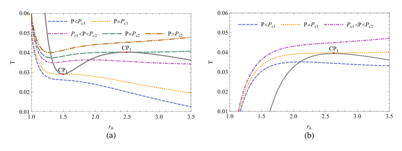
Figure V.1: The solid lines in the figure represent phase transition temperature $T_{p}$, the other lines represent isobaric temperature curve. $CP_{1}$ and $CP_{2}$ are the critical points. We set $Q=1,\alpha=-0.1$ and (a) $a=3$, (b) $a=-1$.

Phase transition will happen when the heat capacity $C_{P}$ goes to infinity,

$$C_{P}=T\left(\frac{\partial S}{\partial T}\right)_{P}=\infty.$$ (V.19)

In other word, phase transition satisfies

$$\left(\frac{\partial T}{\partial S}\right)_{P,\alpha,a,Q}=0.$$ (V.20)

According to Eq. (V.15), we can rewrite Eq. (V.20) as

$$\left(\frac{\partial T}{\partial r_{h}}\right)_{P,\alpha,a,Q}=0.$$ (V.21)

Based on this, we can obtain the relationship between the phase transition pressure $P$ and the horizon radius $r_{h}$, as well as the relationship between the phase transition point temperature $T_{p}$ and the horizon radius $r_{h}$,

$$P=\frac{1}{32\pi r_{h}^{8}}\left(7aQ^{4}-12Q^{2}r_{h}^{4}+8\alpha r_{h}^{5}+4r_{h}^{6}\right),$$ (V.22)

$$T_{p}=\frac{1}{4\pi r_{h}^{7}}\left(2aQ^{4}-4Q^{2}r_{h}^{4}+3\alpha r_{h}^{5}+2r_{h}^{6}\right).$$ (V.23)

One can find the phase transition curves in Figure. V.1. And we will illustrate that poles, $CP_{1}$ and $CP_{2}$, on the phase transition curves are critical points. Here, we reference the relationship of critical points mentioned in critical ,

$$\left(\frac{\partial T}{\partial S}\right)_{P}=\left(\frac{\partial^{2}T}{\partial S^{2}}\right)_{P}=0.$$ (V.24)

According to the analysis in Appendix. A, critical point could be solved by

$$\frac{\partial T_{p}}{\partial S}=0.$$ (V.25)

Due to Eq. (V.15), we can rewrite it as,

$$\left(\frac{\partial T_{p}}{\partial r_{h}}\right)_{\alpha,a,Q}=0.$$ (V.26)

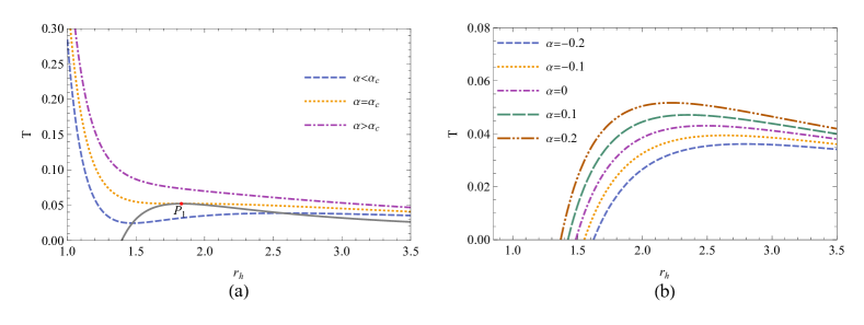
Figure V.2: The solid lines in figure represent critical point curve $T_{cp}$, the other lines represent phase transition curve $T_{p}$. $\alpha$ reaches its critical value at $P_{1}$. We set $Q=1$ and (a) $a=3$, (b) $a=-1$.

Based on this, we could obtain the expression of $\alpha$ and the critical point temperature $T_{cp}$ as following functions,

$$\alpha=\frac{1}{3r_{h}^{5}}\left(-7aQ^{4}+6Q^{2}r_{h}^{4}-r_{h}^{6}\right),$$ (V.27)

$$T_{cp}=\frac{1}{4\pi r_{h}^{7}}\left(-5aQ^{4}+2Q^{2}r_{h}^{4}+r_{h}^{6}\right).$$ (V.28)

One could easily find that in Figure. V.2, there is a critical value of parameter $\alpha$ corresponding to the point $P_{1}$, which two critical points combine into one point. The point $P_{1}$ should meet with

$$\left(\frac{\partial T_{cp}}{\partial r_{h}}\right)_{a,Q}=0.$$ (V.29)

From above equation, we can calculate the value of parameter $a$ and the temperature $T_{co}$ of the combination point as this following formula,

$$a=\frac{r_{h}^{4}}{35Q^{4}}\left(6Q^{2}+r_{h}^{2}\right),$$ (V.30)

$$T_{co}=\frac{4Q^{2}+3r_{h}^{2}}{14\pi r_{h}^{3}}.$$ (V.31)

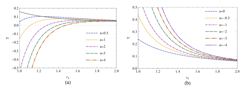
Figure V.3: The solid lines in figure represent combination of critical points $T_{co}$, the other lines represent critical point curve $T_{cp}$. We set $Q=1$ and (a) $a>0$, (b) $a\leq 0$.

As we can see in Figure. V.3, every critical point curve $T_{cp}$ has only one combination point for the case that $a>0$, we can get only one positive real root from Eq. (V.30),

$$r_{h}=\sqrt{\frac{4Q^{4}}{A}+A-2Q^{2}},$$ (V.32)

where

$$A=\left(\frac{35aQ^{4}}{2}-8Q^{6}+\frac{\sqrt{35aQ^{8}\left(35a-32Q^{2}\right)}}{2}\right)^{\frac{1}{3}}.$$ (V.33)

Furthermore, by substituting Eq. (V.32) into Eq. (V.27), one could easily get the function of $\alpha_{c}$ as

$$\alpha_{c}=-\frac{7aQ^{4}}{3\left(\frac{4Q^{4}}{A}+A-2Q^{2}\right)^{5/2}}+\frac{2Q^{2}}{\sqrt{\frac{4Q^{4}}{A}+A-2Q^{2}}}-\frac{\sqrt{\frac{4Q^{4}}{A}+A-2Q^{2}}}{3},$$ (V.34)

where $A$ takes Eq. (V.33).

VI Conclusion and outlook

Firstly, we mathematically discussed the generation of new metric. We found that if multiple interactions do not influence each other and energy momentum tensor $T_{0}^{0}$ is independent from metric to be determined, the solution of metric will conform to linear superposition relationship. Subsequently, we derived the metric of E-H black hole surrounded by PFDM. We plotted the photon orbits and the first and second order images of thin accretion disk, and showed the impact of varying parameter values on results. Finally, we researched the thermodynamics, containing thermodynamic functions, equation of state and phase transition. The result showed that the PFDM parameter will signally affect the criticality.

Looking forward, due to the conservation of angular momentum, black holes formed from the collapse of stars are rarely non-rotating. Therefore, it will be more realistic to consider rotation. Compared to spherically symmetric spacetime, we believe that axially symmetric spacetime is bound to yield more intriguing results in optics. As for the thermodynamics aspect, there are actually more different thermodynamic properties to be researched in the future. For instance, one could calculate the critical exponents criticalexponent1 ; criticalexponent2 . It is meaningful that one could investigate whether thermodynamics of this black hole is similar to Van der Waals system RN-Ads1 ; RN-Ads2 ; Dolan via studying more thermodynamics in detail, like heat capacity, Gibbs free energy and any other thermodynamic phenomena. In fact, there is a interesting phenomenon, Joule-Thomson expansion studied in JTE1 ; JTE2 ; JTE3 . It is hopeful that research the Joule-Thomson expansion of this type of black holes and compare the result with other researchers’. More generally, perhaps using other models of dark matter will lead to more attractive results for us.

Conflicts of interest

The authors declare that there are no conflicts of interest regarding the publication of this paper.

Appendix A Equation of critical point

The function $P\left(S\right)$ is defined to satisfy

$$\frac{\partial T}{\partial S}\left(S,P\left(S\right)\right)=0.$$ (A.1)

Take the derivative of S for both sides of Eq. (A.1), one could get

$$\frac{\partial^{2}T}{\partial S^{2}}+\frac{\partial^{2}T}{\partial S\partial P}\frac{\partial P}{\partial S}=0.$$ (A.2)

Furthermore, consider function $T_{p}\left(S\right)=T\left(S,P\left(S\right)\right)$,

$$\frac{\partial T_{p}}{\partial S}=\frac{\partial T}{\partial S}+\left(\frac{\partial T}{\partial P}\right)_{S}\frac{\partial P}{\partial S}=0.$$ (A.3)

Combine Eq. (A.2) with Eq. (A.3) under the condition $\partial T/\partial S=0$, one get

$$\frac{\partial^{2}T}{\partial S^{2}}=-\frac{\partial^{2}T}{\partial P\partial S}\frac{1}{\left(\frac{\partial T}{\partial P}\right)_{S}}\frac{\partial T_{p}}{\partial S}.$$ (A.4)

Obviously,

$$\frac{\partial T_{p}}{\partial S}=0\quad\Leftrightarrow\quad\frac{\partial^{2}T}{\partial S^{2}}=0,$$ (A.5)

when $\partial T/\partial S=0$.

References

- [1] Albert Einstein. Die feldgleichungen der gravitation. Sitzungsberichte der Königlich Preußischen Akademie der Wissenschaften, pages 844–847, 1915.
- [2] Albert Einstein. Näherungsweise integration der feldgleichungen der gravitation. Sitzungsberichte der Königlich Preußischen Akademie der Wissenschaften, pages 688–696, 1916.
- [3] Albert Einstein. Kosmologische betrachtungen zur allgemeinen relativitätstheorie. Sitzungsberichte der Königlich Preussischen Akademie der Wissenschaften, pages 142–152, 1917.
- [4] Benjamin P Abbott, Richard Abbott, TDe Abbott, MR Abernathy, Fausto Acernese, Kendall Ackley, Carl Adams, Thomas Adams, Paolo Addesso, RX Adhikari, et al. Observation of gravitational waves from a binary black hole merger. Physical review letters, 116(6):061102, 2016.
- [5] David Ball, Chi-kwan Chan, Pierre Christian, Buell T Jannuzi, Junhan Kim, Daniel P Marrone, Lia Medeiros, Feryal Ozel, Dimitrios Psaltis, Mel Rose, et al. First m87 event horizon telescope results. i. the shadow of the supermassive black hole. 2019.
- [6] Kazunori Akiyama, Antxon Alberdi, Walter Alef, Keiichi Asada, Rebecca Azulay, Anne-Kathrin Baczko, David Ball, Mislav Baloković, John Barrett, Dan Bintley, et al. First m87 event horizon telescope results. ii. array and instrumentation. The Astrophysical Journal Letters, 875(1):L2, 2019.
- [7] Event Horizon Telescope Collaboration et al. First m87 event horizon telescope results. iii. data processing and calibration. arXiv preprint arXiv:1906.11240, 2019.
- [8] Kazunori Akiyama, Antxon Alberdi, Walter Alef, Keiichi Asada, Rebecca Azulay, Anne-Kathrin Baczko, David Ball, Mislav Baloković, John Barrett, Dan Bintley, et al. First m87 event horizon telescope results. iv. imaging the central supermassive black hole. The Astrophysical Journal Letters, 875(1):L4, 2019.
- [9] Kazunori Akiyama, Antxon Alberdi, Walter Alef, Keiichi Asada, Rebecca Azulay, Anne-Kathrin Baczko, David Ball, Mislav Baloković, John Barrett, Dan Bintley, et al. First m87 event horizon telescope results. v. physical origin of the asymmetric ring. The Astrophysical Journal Letters, 875(1):L5, 2019.
- [10] Daniela Magos and Nora Breton. Thermodynamics of the euler-heisenberg-ads black hole. Physical Review D, 102(8):084011, 2020.
- [11] Xu Ye, Zi-Qing Chen, Ming-Da Li, and Shao-Wen Wei. Qed effects on phase transition and ruppeiner geometry of euler-heisenberg-ads black holes. Chinese Physics C, 46(11):115102, 2022.
- [12] Heng Dai, Zixu Zhao, and Shuhang Zhang. Thermodynamic phase transition of euler-heisenberg-ads black hole on free energy landscape. Nuclear Physics B, 991:116219, 2023.
- [13] Guan-Ru Li, Sen Guo, and En-Wei Liang. High-order qed correction impacts on phase transition of the euler-heisenberg ads black hole. Physical Review D, 106(6):064011, 2022.
- [14] Hiroki Yajima and Takashi Tamaki. Black hole solutions in euler-heisenberg theory. Physical Review D, 63(6):064007, 2001.
- [15] Xiao-Xiong Zeng, Ke-Jian He, Guo-Ping Li, En-Wei Liang, and Sen Guo. Qed and accretion flow models effect on optical appearance of euler–heisenberg black holes. The European Physical Journal C, 82(8):764, 2022.
- [16] Werner Heisenberg and Heinrich Euler. Folgerungen aus der diracschen theorie des positrons. Zeitschrift für Physik, 98(11-12):714–732, 1936.
- [17] Ming-Hsun Li and Kwei-Chou Yang. Galactic dark matter in the phantom field. Physical Review D, 86(12):123015, 2012.
- [18] VV1966820 Kiselev. Quintessence and black holes. Classical and Quantum Gravity, 20(6):1187, 2003.
- [19] VV Kiselev. Quintessential solution of dark matter rotation curves and its simulation by extra dimensions. arXiv preprint gr-qc/0303031, 2003.
- [20] Anish Das, Ashis Saha, and Sunandan Gangopadhyay. Investigation of circular geodesics in a rotating charged black hole in the presence of perfect fluid dark matter. Classical and Quantum Gravity, 38(6):065015, 2021.
- [21] F Rahaman, KK Nandi, A Bhadra, M Kalam, and K Chakraborty. Perfect fluid dark matter. Physics Letters B, 694(1):10–15, 2010.
- [22] J-P Luminet. Image of a spherical black hole with thin accretion disk. Astronomy and Astrophysics, vol. 75, no. 1-2, May 1979, p. 228-235., 75:228–235, 1979.
- [23] Yu-Xiang Huang, Sen Guo, Yu-Hao Cui, Qing-Quan Jiang, and Kai Lin. Influence of accretion disk on the optical appearance of the kazakov-solodukhin black hole. Physical Review D, 107(12):123009, 2023.
- [24] Malihe Heydari-Fard, Sara Ghassemi Honarvar, and Mohaddese Heydari-Fard. Thin accretion disc luminosity and its image around rotating black holes in perfect fluid dark matter. Monthly Notices of the Royal Astronomical Society, 521(1):708–716, 2023.
- [25] Shi-Jie Ma, Tian-Chi Ma, Jian-Bo Deng, and Xian-Ru Hu. Shadow of schwarzschild black hole in the cold dark matter halo. Modern Physics Letters A, 38(24n25):2350104, 2023.
- [26] Stephen W Hawking and Don N Page. Thermodynamics of black holes in anti-de sitter space. Communications in Mathematical Physics, 87:577–588, 1983.
- [27] Andrew Chamblin, Roberto Emparan, Clifford V Johnson, and Robert C Myers. Charged ads black holes and catastrophic holography. Physical Review D, 60(6):064018, 1999.
- [28] Andrew Chamblin, Roberto Emparan, Clifford V Johnson, and Robert C Myers. Holography, thermodynamics, and fluctuations of charged ads black holes. Physical Review D, 60(10):104026, 1999.
- [29] David Kastor, Sourya Ray, and Jennie Traschen. Enthalpy and the mechanics of ads black holes. Classical and Quantum Gravity, 26(19):195011, 2009.
- [30] Brian P Dolan. The cosmological constant and the black hole equation of state. arXiv preprint arXiv:1008.5023, 2010.
- [31] He-Xu Zhang, Yuan Chen, Tian-Chi Ma, Peng-Zhang He, and Jian-Bo Deng. Bardeen black hole surrounded by perfect fluid dark matter. Chinese Physics C, 45(5):055103, 2021.
- [32] ID Novikov and KS Thorne. Black holes, edited by c. dewitt and bs dewitt, 1973.
- [33] Don N Page and Kip S Thorne. Disk-accretion onto a black hole. time-averaged structure of accretion disk. The Astrophysical Journal, 191:499–506, 1974.
- [34] David Kubizňák and Robert B Mann. P- v criticality of charged ads black holes. Journal of High Energy Physics, 2012(7):1–25, 2012.
- [35] Robert M Wald. The thermodynamics of black holes. Living reviews in relativity, 4:1–44, 2001.
- [36] Manuel E Rodrigues, Marcos V de S Silva, and Henrique A Vieira. Bardeen-kiselev black hole with a cosmological constant. Physical Review D, 105(8):084043, 2022.
- [37] Mohammad Reza Alipour, Mohammad Ali S Afshar, Saeed Noori Gashti, and Jafar Sadeghi. Topological classification and black hole thermodynamics. arXiv preprint arXiv:2305.05595, 2023.
- [38] Özgür Ökcü and Ekrem Aydıner. Joule–thomson expansion of the charged ads black holes. The European Physical Journal C, 77:1–7, 2017.
- [39] Cong Li, Pengzhang He, Ping Li, and Jian-Bo Deng. Joule–thomson expansion of the bardeen-ads black holes. General Relativity and Gravitation, 52:1–10, 2020.
- [40] MB Tataryn and MM Stetsko. Thermodynamics of a static electric-magnetic black hole in einstein-born-infeld-ads theory with different horizon geometries. General Relativity and Gravitation, 53(8):72, 2021.