Thin layer axion dynamo

Abstract

We study interacting classical magnetic and pseudoscalar fields in frames of the axion electrodynamics. A large scale pseudoscalar field can be the coherent superposition of axions or axion like particles. We consider the evolution of these fields in a thin spherical layer. Decomposing the magnetic field into the poloidal and toroidal components, we take into account their symmetry properties. The dependence of the pseudoscalar field on the latitude is accounted for the induction equation. Then, we derive the dynamo equations in the low mode approximation. The nonlinear evolution equations for the harmonics of the magnetic and pseudoscalar fields are solved numerically. As an application, we consider a dense axion star embedded in solar plasma. The behavior of the harmonics and their typical oscillations frequencies are obtained. We suggest that such small objects consisting of axions and confined magnetic fields can cause the recently observed flashes in solar corona contributing to its heating.

1 Introduction

The major fraction of the universe mass, called dark matter, almost does not interact with light. Dark matter forms the halo throughout the Galaxy, where it is distributed more or less uniformly. Nevertheless, the presence of a measurable fraction of dark matter in the vicinity of usual stars, like the Sun, is not excluded [1]. Moreover, a possible dark matter detection was recently reported in Ref. [2]. In principle, dark matter can form clusters and stars [3] which are not related to baryonic astronomical objects. Thus, one can consider spatially confined dark matter structures.

The origin and the content of dark matter is unclear. Axions and axion like particles (ALP) are considered as the most plausible candidates for dark matter [4]. Besides the gravitational interaction, these particles interact rather weakly with electromagnetic fields [5]. It can lead to numerous phenomena, like the emission of strong electromagnetic radiation, in collisions of axion stars with, e.g., neutron stars (see, e.g., Ref. [3]).

In frames of the axion magneto-hydrodynamics (MHD), a magnetic field was mentioned in Ref. [6] to be unstable since the time dependent axion wavefunction acts as the $\alpha$-dynamo parameter. The axion MHD in the early universe was studied in Refs. [7, 8]. The evolution of large scale magnetic fields in the presence of inhomogeneous axions in the mean field approximation was considered in Ref. [9].

The axion dynamo in neutron stars was developed in Ref. [10]. However, the induction equation used in Ref. [10] does not account for the coordinate dependence of the axion wavefunction. The most complete induction equation, accounting for the axions spatial inhomogeneity, was derived recently in Ref. [11] (see also Appendix A). Based on this equation, in Ref. [11], we analyzed the mixing between two Chern-Simons waves in one dimensional geometry, as well as a more sophisticated three dimensional (3D) case involving the Hopf fibration. The emission of photons by axions in strong magnetic fields in the vicinity of neutron stars was studied in Ref. [12].

In the present work, based on the results of Ref. [11], we develop a 3D axion dynamo in an axion spherical star. We start in Sec. 2 with deriving of the differential equations for the poloidal and toroidal magnetic fields, as well as for the axion wavefunction. Then, in Sec. 3, we consider the application of our results for the evolution of magnetic fields in an axion star embedded in solar plasma. Finally, we conclude in Sec. 4. Some phenomenological consequences of our results are also discussed in Sec. 4. The modified induction equation accounting for the spatially inhomogeneous axion wavefunction is rederived in Appendix A. The system of nonlinear differential equations for the harmonics of magnetic and pseudoscalar fields are obtained in Appendix B.

2 Axion dynamo

In this section, we derive the main dynamo equations in frames of the axion MHD in the low mode approximation. We consider the dynamo action in a thin spherical layer.

The evolution of the magnetic field $\mathbf{B}$ under the influence of the external inhomogeneous pseudoscalar field $\varphi$ obeys the equation (see Eq. (A.7) and Ref. [11]),

$$\dot{\mathbf{B}}=\nabla\times\left[\mathbf{b}\times(\nabla\times\mathbf{B})+\alpha\mathbf{B}-\eta(\nabla\times\mathbf{B})\right].$$ (2.1)

If the pseudoscalar field is a coherent superposition of axions, $\alpha=g_{a\gamma}\eta\dot{\varphi}$ is the $\alpha$-dynamo parameter, $\mathbf{b}=g_{a\gamma}\eta^{2}\nabla\varphi$ is the axial vector accounting for the spatial inhomogeneity of $\varphi$, $\eta$ is the magnetic diffusion coefficient, and $g_{a\gamma}$ is the axion-photon coupling constant. In Eq. (2.1), a dot means the time derivative. The molecular contribution to the magnetic diffusion coefficient is $\eta=\sigma^{-1}$, where $\sigma$ is the electric conductivity. However, the turbulent magnetic diffusion can be much sizable than the molecular one.

The induction Eq. (2.1) should be supplied with the inhomogeneous Klein-Gordon equation for $\varphi$ [9, 11],

$$\ddot{\varphi}-\Delta\varphi+m^{2}\varphi=g_{a\gamma}(\mathbf{EB}),$$ (2.2)

where $m$ is the mass of $\varphi$. The expression for the electric field is

$$\mathbf{E}=\eta(\nabla\times\mathbf{B})-\alpha\mathbf{B}-[\mathbf{b}\times(\nabla\times\mathbf{B})],$$ (2.3)

which is given in Eq. (A.6) (see also Refs. [9, 11]).

We consider the fields $\mathbf{B}$ and $\varphi$ inside the spherical volume which can be an axion star. All the quantities in Eqs. (2.1) and (2.2) are supposed to be axially symmetric. For example, $\alpha=\alpha(r,\theta,t)$, $\mathbf{b}=b_{r}\mathbf{e}_{r}+b_{\theta}\mathbf{e}_{\theta}$, and $b_{r,\theta}=b_{r,\theta}(r,\theta,t)$. Here we use the orthonormal basis in spherical coordinates $\mathbf{e}_{i}$, $i=r,\theta,\phi$. The $\alpha$-dynamo parameter should by antisymmetric with respect to the equatorial plane, $\alpha(r,\pi-\theta,t)=-\alpha(r,\theta,t)$, since $\varphi$ is pseudoscalar. The magnetic field is separated into the poloidal $\mathbf{B}_{p}$ and toroidal $\mathbf{B}_{t}$ components, $\mathbf{B}=\mathbf{B}_{p}+\mathbf{B}_{t}$. We take that $\mathbf{B}_{p}=\nabla\times(A\mathbf{e}_{\phi})$ and $\mathbf{B}_{t}=B\mathbf{e}_{\phi}$. The new functions $A$ and $B$ have the following symmetry properties: $A(r,\pi-\theta,t)=A(r,\theta,t)$ and $B(r,\pi-\theta,t)=-B(r,\theta,t)$.

Making tedious but straightforward calculations based on Eq. (2.1), we get the equations for $A$ and $B$,

$$\frac{\partial A}{\partial t}= -g_{a\gamma}\eta^{2}\frac{1}{r}\left[\frac{\partial\varphi}{\partial r}\frac{\partial}{\partial r}\left(rB\right)+\frac{1}{r\sin\theta}\frac{\partial\varphi}{\partial\theta}\frac{\partial}{\partial\theta}\left(\sin\vartheta B\right)\right]+g_{a\gamma}\eta B\frac{\partial\varphi}{\partial t}+\eta\Delta^{\prime}A,$$

$$\frac{\partial B}{\partial t}= g_{a\gamma}\eta^{2}\frac{1}{r}\left[\frac{\partial}{\partial r}\left(r\frac{\partial\varphi}{\partial r}\Delta^{\prime}A\right)+\frac{1}{r}\frac{\partial}{\partial\theta}\left(\frac{\partial\varphi}{\partial\theta}\Delta^{\prime}A\right)\right]$$

$$-g_{a\gamma}\eta\frac{1}{r}\left[\frac{\partial}{\partial r}\left(\frac{\partial\varphi}{\partial t}\frac{\partial}{\partial r}\left(rA\right)\right)+\frac{1}{r}\frac{\partial}{\partial\theta}\left(\frac{1}{\sin\theta}\frac{\partial\varphi}{\partial t}\frac{\partial}{\partial\theta}\left(\sin\theta A\right)\right)\right]+\eta\Delta^{\prime}B,$$ (2.4)

where $\Delta^{\prime}=\Delta-\tfrac{1}{r^{2}\sin^{2}\theta}=\tfrac{1}{r^{2}}\tfrac{\partial}{\partial r}\left(r^{2}\tfrac{\partial}{\partial r}\right)+\tfrac{1}{r^{2}\sin\theta}\tfrac{\partial}{\partial\theta}\left(\sin\theta\tfrac{\partial}{\partial\theta}\right)-\tfrac{1}{r^{2}\sin^{2}\theta}$ is the modified Laplace operator. Analogously, we transform Eq. (2.2) to the form,

$$\frac{\partial^{2}\varphi}{\partial t^{2}}+m^{2}\varphi-\frac{1}{r^{2}}\frac{\partial\varphi}{\partial r}\left(r^{2}\frac{\partial\varphi}{\partial r}\right)-\frac{1}{r^{2}\sin\theta}\frac{\partial}{\partial\theta}\left(\sin\theta\frac{\partial\varphi}{\partial\theta}\right)\\ =g_{a\gamma}\eta\left[\frac{1}{r^{2}\sin^{2}\theta}\frac{\partial}{\partial\theta}\left(\sin\vartheta B\right)\frac{\partial}{\partial\theta}\left(\sin\vartheta A\right)+\frac{1}{r^{2}}\frac{\partial}{\partial r}\left(rB\right)\frac{\partial}{\partial r}\left(rA\right)-B\Delta^{\prime}A\right].$$ (2.5)

To derive Eq. (2.5) we keep only the first term in the right hand side of Eq. (2.3) to guarantee that the result is linear in $g_{a\gamma}$.

Now, following Ref. [13], we assume that the fields $(A,B,\varphi)$ evolve in a thin layer between $R$ and $R+\mathrm{d}r$, where $R$ is the typical size of an axion star and $\mathrm{d}r\ll R$. In this case, the radial dependence of the functions can be neglected. Therefore, we can replace $r\to R$ and $\frac{\partial}{\partial r}\to 0$ in Eqs. (2) and (2.5).

Using the dimensionless variables

$$\mathcal{A}=g_{a\gamma}A,\quad\mathcal{B}=g_{a\gamma}RB,\quad\Phi=\frac{g_{a\gamma}\eta}{R}\varphi,\quad\tau=\frac{\eta t}{R^{2}},$$ (2.6)

we rewrite Eqs. (2) and (2.5) in the form,

$$\frac{\partial\mathcal{A}}{\partial\tau}= -\frac{\partial\Phi}{\partial\theta}\left[\frac{\partial\mathcal{B}}{\partial\theta}+\cot\theta\mathcal{B}\right]+\frac{\partial\Phi}{\partial\tau}\mathcal{B}+\frac{\partial^{2}\mathcal{A}}{\partial\theta^{2}}+\cot\theta\frac{\partial\mathcal{A}}{\partial\theta}-\frac{\mathcal{A}}{\sin^{2}\theta},$$

$$\frac{\partial\mathcal{B}}{\partial\tau}= \frac{\partial^{2}\Phi}{\partial\theta^{2}}\left(\frac{\partial^{2}\mathcal{A}}{\partial\theta^{2}}+\cot\theta\frac{\partial\mathcal{A}}{\partial\theta}-\frac{\mathcal{A}}{\sin^{2}\theta}\right)$$

$$+\frac{\partial\Phi}{\partial\theta}\left(\frac{\partial^{3}\mathcal{A}}{\partial\theta^{3}}+\cot\theta\frac{\partial^{2}\mathcal{A}}{\partial\theta^{2}}-\frac{2}{\sin^{2}\theta}\frac{\partial\mathcal{A}}{\partial\theta}+\frac{2\cot\theta}{\sin^{2}\theta}\mathcal{A}\right)$$

$$-\frac{\partial^{2}\Phi}{\partial\tau\partial\theta}\left(\frac{\partial\mathcal{A}}{\partial\theta}+\cot\theta\mathcal{A}\right)-\frac{\partial\Phi}{\partial\tau}\left(\frac{\partial^{2}\mathcal{A}}{\partial\theta^{2}}+\cot\theta\frac{\partial\mathcal{A}}{\partial\theta}-\frac{\mathcal{A}}{\sin^{2}\theta}\right)$$

$$+\frac{\partial^{2}\mathcal{B}}{\partial\theta^{2}}+\cot\theta\frac{\partial\mathcal{B}}{\partial\theta}-\frac{\mathcal{B}}{\sin^{2}\theta},$$

$$\frac{\partial^{2}\Phi}{\partial\tau^{2}}= -\mu^{2}\Phi+\kappa^{2}\left(\frac{\partial^{2}\Phi}{\partial\theta^{2}}+\cot\theta\frac{\partial\Phi}{\partial\theta}\right)$$

$$+\left(\frac{\partial\mathcal{B}}{\partial\theta}+\cot\theta\mathcal{B}\right)\left(\frac{\partial\mathcal{A}}{\partial\theta}+\cot\theta\mathcal{A}\right)+\mathcal{A}\mathcal{B}$$

$$-\mathcal{B}\left(\frac{\partial^{2}\mathcal{A}}{\partial\theta^{2}}+\cot\theta\frac{\partial\mathcal{A}}{\partial\theta}-\frac{\mathcal{A}}{\sin^{2}\theta}\right),$$ (2.7)

where $\mu=mR^{2}/\eta$ is the dimensionless axion mass and $\kappa=R/\eta$ is the effective wave vector.

According to Ref. [14], we decompose the dimensionless functions $(\mathcal{A},\mathcal{B},\Phi)$ into the harmonics,

$$\mathcal{A} =a_{1}(\tau)\sin\theta+a_{2}(\tau)\sin 3\theta+\dotsc,$$

$$\mathcal{B} =b_{1}(\tau)\sin 2\theta+b_{2}(\tau)\sin 4\theta+\dotsc,$$

$$\Phi =\phi_{1}(\tau)\sin 2\theta+\phi_{2}(\tau)\sin 4\theta+\dotsc,$$ (2.8)

where the coefficients $a_{1,2}$, $b_{1,2}$, and $\phi_{1,2}$ are the functions of $\tau$ only. The decomposition in Eq. (2) obeys the symmetry conditions specified earlier. Note that use the low mode approximation in Eq. (2) considering only two first harmonics. Substituting Eq. (2) to Eq. (2), we get the system of nonlinear ordinary differential equations, which is provided in Eq. (B), for the functions $a_{1,2}$, $b_{1,2}$, and $\phi_{1,2}$.

3 Axion dynamo in solar plasma

Our main goal is to study the influence of an external pseudoscalar field on the evolution of magnetic fields. For this purpose to assume the existence of a spherical object consisting of coherent axions where a seed magnetic field is present. An axion star is an example of such a structure. We study the case of a dense axion star. Such a star was found in Ref. [15] be stable if its radius $R\sim(10^{-11}-10^{-10})R_{\odot}=(0.7-7)\,\text{cm}$ or $R\gtrsim 10^{-4}R_{\odot}=70\,\text{km}$. The energy density of axions in a dense axion star is $\rho\lesssim m^{2}f_{a}^{2}$ [3], where $f_{a}=\tfrac{\alpha_{\mathrm{em}}}{2\pi g_{a\gamma}}$ is the Peccei–Quinn constant and $\alpha_{\mathrm{em}}=7.3\times 10^{-3}$ is the fine structure constant.

We study the contribution of axions to the dynamics of magnetic fields which can be present in solar plasma. We take the small radius of an axion star $R=0.7\,\text{cm}$ [15]. The solar magnetic diffusion coefficient was mentioned in Ref. [16, p. 370] to be mainly turbulent one. We take that $\eta=10^{10}\,\text{cm}^{2}\cdot\text{s}^{-1}$, which is close to the observed value given in Ref. [17]. The effective mass and the wave number are $\mu=7.5\times 10^{-1}$ and $\kappa=2.1$. Here, we take that $m=10^{-5}\,\text{eV}$.

We suppose that $\dot{\varphi}(t=0)=0$ and the energy density of axions is $\rho=10^{-2}m^{2}f_{a}^{2}$. In this case, the initial value of $\rho$ is

$$\rho_{0}=\frac{1}{2}\left[(\nabla\varphi_{0})^{2}+m^{2}\varphi_{0}^{2}\right]\approx\frac{\mu^{2}\left\langle(\partial_{\theta}\Phi_{0})^{2}\right\rangle}{2g_{a\gamma}^{2}R^{2}},$$ (3.1)

where we use Eq. (2.6) and the fact that $\mu^{2}\ll\kappa^{2}$. The fact that $|\nabla\varphi_{0}|$ term is dominant in Eq. (3.1) shows the importance the axion inhomogeneity in the system. Supposing that $\phi_{2}(0)=0$, as well as taking that $\rho_{0}\approx 10^{-2}m^{2}f_{a}^{2}$ and $\left\langle\cos 2\theta\right\rangle=\tfrac{1}{2}$ in Eq. (3.1), we obtain the part of the initial condition for the system in Eq. (B),

$$\phi_{1}(0)=10^{-1}\frac{\alpha_{\mathrm{em}}mR}{2\pi\kappa}=2\times 10^{-2},$$ (3.2)

and $\phi_{2}(0)=0$, $\dot{\phi}_{1,2}(0)=0$.

The initial condition for $\mathcal{A}$ and $\mathcal{B}$ can be obtained using Eq. (2.6),

$$a_{1}(0)=1.4\times 10^{-17}\left(\frac{B_{\mathrm{pol}}^{(0)}}{\mathrm{kG}}\right),\quad b_{1}(0)=1.4\times 10^{-17}\left(\frac{B_{\mathrm{tor}}^{(0)}}{\mathrm{kG}}\right),$$ (3.3)

and $a_{2}(0)=b_{2}(0)=0$. In Eq. (3.3), $B_{\mathrm{pol,tor}}^{(0)}$ are the seed poloidal and toroidal magnetic fields. We take that $B_{\mathrm{pol,tor}}^{(0)}=4\,\text{kG}$ [18]. After setting the initial condition, we can solve the system in Eq. (B).

In Fig. 1, we show the behavior of the system in solar plasma when only the seed poloidal magnetic field is present, i.e. $a_{1}(0)\neq 0$ and $b_{1}(0)=0$ in Eq. (3.3). One can see in Figs. 1 and 1 the evolution of the harmonics $a_{1,2}$ and $b_{1,2}$. The insets in Figs. 1 and 1 represent the behavior of these functions in small evolution times, when the initial condition is visible.

The spectra of $a_{1,2}$ and $b_{1,2}$ are shown in Figs. 1 and 1. The poloidal component can be measured since it extends to outer regions of an axion star. The typical frequency of $a_{1}$ oscillations, in Fig. 1, is $f\sim 10^{10}\,\text{Hz}$. Here we take the second peak in the spectrum of $a_{1}$. Such oscillations frequency implies the validity of the causality condition, $fR<1$. Moreover, the MHD approximation, $\eta^{-1}\gg f$, is also valid in this case.

We depict the evolution of the total magnetic energy density in Fig. 1,

$$\rho_{\mathrm{B}}(\theta,t)=\frac{\mathbf{B}^{2}}{2}\propto\left(\frac{\partial\mathcal{A}}{\partial\theta}+\cot\theta\mathcal{A}\right)^{2}+\mathcal{A}^{2}+\mathcal{B}^{2},$$ (3.4)

in a short time interval to demonstrate its distribution over the $\text{Latitude}=90^{\circ}\times\left(1-2\theta/\pi\right)$. It is the analogue of a ‘butterfly’ diagram in solar physics (see, e.g., Ref. [16, p. 377]).

The evolution of the harmonics of the pseudoscalar field is present in Fig. 1. Both harmonics of $\varphi$ have approximately equal amplitudes. It demonstrates the importance of keeping the coordinate dependence of $\varphi$ both in Eqs. (2.1) and (2.2). One can see that frequencies of $\varphi$ oscillations are much smaller than those of the magnetic fields.

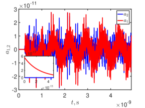
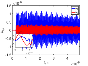
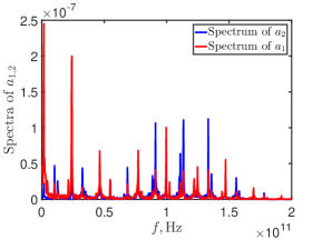
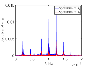
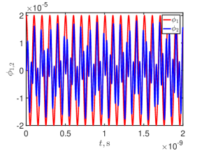
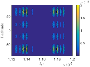
Figure 1: The evolution of the magnetic and pseudoscalar fields inside the axion star embedded in solar plasma. (a) The time evolution of the poloidal harmonics $a_{1,2}$. (b) The behavior of toroidal harmonics $b_{1,2}$ versus time. (c) The spectra of $a_{1,2}$. (d) The spectra of $b_{1,2}$. (e) The harmonics $\phi_{1,2}$ of the pseudoscalar field. (f) The total magnetic energy density in Eq. (3.4). We take that $B_{\mathrm{pol}}^{(0)}=4\,\text{kG}$ and $B_{\mathrm{tor}}^{(0)}=0$.

In Fig. 2, we show the evolution of the system when only a seed toroidal magnetic field is present initially, i.e. we take that $b_{1}(0)\neq 0$ and $a_{1}(0)=0$. Now, the strength of the seed toroidal field is the same as for the poloidal one in Fig. 1, i.e. $B_{\mathrm{tor}}^{(0)}=4\,\text{kG}$. The initial condition for the harmonics can be seen in the insets in Figs. 2 and 2. The behavior of the magnetic fields and $\varphi$ qualitatively resembles that in Fig. 1.

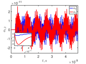
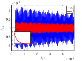
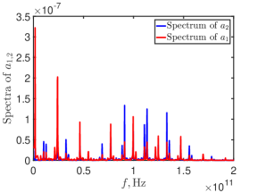
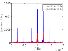
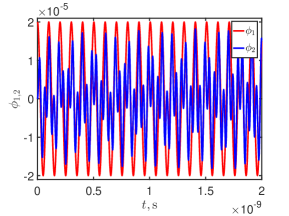
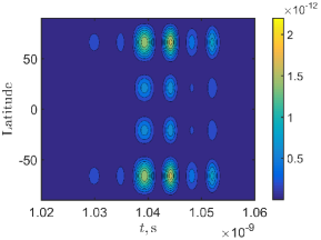
Figure 2: The same as in Fig. 1 for $B_{\mathrm{pol}}^{(0)}=0$ and $B_{\mathrm{tor}}^{(0)}=4\,\text{kG}$.

We can see in Figs. 1 and 2 that the evolution of the pseudoscalar field is unaffected by the magnetic field. We also notice in Figs. 1, 1, 2, and 2 that the magnetic fields are amplified by the $\alpha$-dynamo driven by the inhomogeneous axion $\varphi$. After the amplification, the magnetic field enters to the oscillating regime. It should be mentioned that, in Figs. 1 and 2, the frequency of the first peaks in the spectra of $a_{1}$, which are the maximal ones, is $\sim 10^{9}\,\text{Hz}$.

4 Conclusion

In the present work, we have studied the simultaneous evolution of the magnetic and pseudoscalar macroscopic fields. The latter can be a coherent superposition of axions or ALP. This system obeys the axion electrodynamics equations which result from the Lagrangian in Eq. (A.1).

In Sec. 2, based on the axion electrodynamics Eqs. (A.2)-(A.5), we have derived the modified induction Eq. (2.1) (see also Ref. [11]) for the magnetic field $\mathbf{B}$, which accounts for the inhomogeneity of the pseudoscalar field, $\nabla\varphi\neq 0$. Equation (2.1) is completed with the Klein-Gordon Eq. (2.2) with the nonzero right hand side describing the interaction between $\varphi$ and the electromagnetic field.

Then, we have developed the axion dynamo in a thin spherical layer. Using the symmetry properties of the poloidal and toroidal magnetic fields, as well as those of $\varphi$, and neglecting the radial dependence of the fields, which is a standard dynamo approximation (see, e.g., Ref. [13]), we have derived the full set of the evolution equations. These equations have been rewritten in the dimensionless variables in Eq. (2). We have used the low mode approximation, accounting for two harmonics (see Ref. [14]), in Eq. (2) to reduce the general evolution equations to the system of nonlinear ordinary differential equations. The details are present in Appendix B.

In Sec. 3, we have studied the application of our results for the description of the magnetic field evolution inside a small axion star embedded in solar plasma. For this purpose, we have considered a dense axion spherical structure with $R\sim 1\,\text{cm}$, which was predicted in Ref. [15]. The seed magnetic field has been taken as $4\,\text{kG}$. We have considered the turbulent magnetic diffusion coefficient corresponding to the observational value [17].

We have obtained that the magnetic field enters to the oscillations regime. The typical frequency of magnetic field oscillations is $\sim 10^{10}\,\text{Hz}$. This frequency guarantees to validity of both the MHD approximation and the causality condition. Such frequencies are covered by the modern solar radio telescopes (see, e.g., Ref. [20]). Thus, potentially the related electromagnetic radiation can be observed.

When such small axionic objects decay, the confined energy of oscillating magnetic fields is liberated as electromagnetic waves. Spatially localized electromagnetic flashes with the frequency $f\lesssim 160\,\text{MHz}$ were reported in Ref. [19] to be a possible source of the solar corona heating. This frequency is slightly below our prediction, especially if we consider the greatest first peaks in the spectra of $a_{1}$ in Figs. 1 and 2. The connection of the observational data in Ref. [19] with the annihilation of dark matter nuggets [21] was discussed in Ref. [22]. The review of solar radio emission caused by the dark matter is given in Ref. [23]. We suggest that small size axion stars, which contain the internal oscillating magnetic fields, described in the present work, can be a possible explanation of flashes in the Sun observed in Ref. [19].

Appendix A Derivation of the modified induction equation

The axion electrodynamics results from the following Lagrangian [7]:

$$\mathcal{L}=-\frac{1}{4}F_{\mu\nu}F^{\mu\nu}+\frac{1}{2}(\partial_{\mu}\varphi\partial^{\mu}\varphi-m^{2}\varphi^{2})-\frac{g_{a\gamma}\varphi}{4}F_{\mu\nu}\tilde{F}^{\mu\nu}-A^{\mu}J_{\mu},$$ (A.1)

where $F_{\mu\nu}=(\mathbf{E},\mathbf{B})$ is the electromagnetic field tensor, $\tilde{F}_{\mu\nu}=\tfrac{1}{2}\varepsilon_{\mu\nu\lambda\rho}F^{\lambda\rho}$ is the dual tensor, $A^{\mu}$ is the electromagnetic field potential, $J^{\mu}=(\rho,\mathbf{J})$ is the external current. The modified Maxwell equations, coming from Eq. (A.1), have the form [9],

$$(\nabla\times\mathbf{B}) =\frac{\partial\mathbf{E}}{\partial t}+\mathbf{J}+g_{a\gamma}\mathbf{B}\frac{\partial\varphi}{\partial t}+g_{a\gamma}(\nabla\varphi\times\mathbf{E}),$$ (A.2)

$$(\nabla\times\mathbf{E}) =-\frac{\partial\mathbf{B}}{\partial t},$$ (A.3)

$$(\nabla\cdot\mathbf{E}) =-g_{a\gamma}(\mathbf{B}\cdot\nabla)\varphi+\rho,$$ (A.4)

$$(\nabla\cdot\mathbf{B}) =0.$$ (A.5)

We suppose that plasma is electroneutral, i.e. $\rho=0$ in Eq. (A.4). Equation (A.2) should be completed by the Ohm’s law $\mathbf{J}=\eta^{-1}\mathbf{E}$, where we omit the advection term since we study a slowly rotating axion star. Such a term was accounted for in Ref. [10]. Moreover, we neglect the displacement current $\frac{\partial\mathbf{E}}{\partial t}$ with respect to the Ohmic current in Eq. (A.2), which is a usual MHD approximation.

After these assumptions, Eq. (A.2) becomes algebraic for the electric field. The electric field can be found in the form [9, 11],

$$\mathbf{E}=\eta(\nabla\times\mathbf{B})-g_{a\gamma}\eta\frac{\partial\varphi}{\partial t}\mathbf{B}-g_{a\gamma}\eta^{2}[\nabla\varphi\times(\nabla\times\mathbf{B})],$$ (A.6)

which coincides with Eq. (2.3). Note that we keep only the terms linear in the coupling constant $g_{a\gamma}$ in Eq. (A.6).

Based on Eqs. (A.3) and (A.6), we obtain the modified induction equation for the magnetic field [9, 11],

$$\frac{\partial\mathbf{B}}{\partial t}=\nabla\times\left[g_{a\gamma}\eta^{2}\nabla\varphi\times(\nabla\times\mathbf{B})+g_{a\gamma}\eta\frac{\partial\varphi}{\partial t}\mathbf{B}-\eta(\nabla\times\mathbf{B})\right],$$ (A.7)

which is represented in Eq. (2.1). Note that $\mathbf{B}$ in Eq. (A.7) automatically satisfies Eq. (A.5), i.e. it is divergenceless.

Appendix B Differential equations for the harmonics

In this appendix, we derive the system of ordinary differential equations for the evolution of the coefficients $a_{1,2}$, $b_{1,2}$, and $\phi_{1,2}$.

For this purpose, we insert Eq. (2) into Eq. (2). Then, we multiply each equation by the corresponding function $\sin n\theta$, where $n=1,\dots 4$, and integrate the result, $\tfrac{2}{\pi}\smallint_{0}^{\pi}\dots\mathrm{d}\theta$, taking into account the orthonormality condition,

$$\frac{2}{\pi}\int_{0}^{\pi}\sin(n\theta)\sin(l\theta)\mathrm{d}\theta=\delta_{nl},$$ (B.1)

where $n,l=1,\dots 4$.

Finally, we obtain the following nonlinear differential equations:

$$\dot{a}_{1}= -2(a_{1}+a_{2})+\frac{2}{\pi}\bigg{[}-\frac{64}{15}b_{1}\phi_{1}-\frac{1024}{63}b_{2}\phi_{2}+\frac{16}{15}b_{1}\psi_{1}+\frac{64}{63}b_{2}\psi_{2}-\frac{32}{105}b_{1}\psi_{2}$$

$$-\frac{32}{105}b_{2}\psi_{1}+\frac{512}{105}b_{1}\phi_{2}+\frac{128}{105}b_{2}\phi_{1}\bigg{]},$$

$$\dot{a}_{2}= -12a_{2}+\frac{2}{\pi}\bigg{[}-\frac{64}{35}b_{1}\phi_{1}-\frac{20992}{3465}b_{2}\phi_{2}+\frac{16}{21}b_{1}\psi_{1}+\frac{64}{165}b_{2}\psi_{2}+\frac{32}{45}b_{1}\psi_{2}$$

$$+\frac{32}{45}b_{2}\psi_{1}-\frac{256}{105}b_{1}\phi_{2}-\frac{2176}{315}b_{2}\phi_{1}\bigg{]},$$

$$\dot{b}_{1}= -2(3b_{1}+2b_{2})+\frac{2}{\pi}\bigg{[}\frac{592}{105}a_{2}\psi_{1}+\frac{608}{315}a_{2}\psi_{2}+\frac{288}{7}a_{2}\phi_{2}+\frac{352}{105}a_{1}\psi_{2}+\frac{304}{105}a_{2}\phi_{1}$$

$$+\frac{112}{15}a_{1}\phi_{1}-\frac{608}{105}a_{1}\phi_{2}+\frac{16}{15}a_{1}\psi_{1}\bigg{]},$$

$$\dot{b}_{2}= -20b_{2}+\frac{2}{\pi}\bigg{[}\frac{1888}{315}a_{2}\psi_{1}+\frac{11584}{3465}a_{2}\psi_{2}+\frac{294592}{3465}a_{2}\phi_{2}+\frac{64}{63}a_{1}\psi_{2}+\frac{288}{7}a_{2}\phi_{1}$$

$$-\frac{608}{105}a_{1}\phi_{1}+\frac{1984}{63}a_{1}\phi_{2}-\frac{416}{105}a_{1}\psi_{1}\bigg{]},$$

$$\dot{\psi}_{1}= -(\mu^{2}+2\kappa^{2})\phi_{1}+\frac{2}{\pi}\left[\frac{6688}{315}a_{2}b_{2}-\frac{32}{15}a_{1}b_{2}+\frac{2096}{105}a_{2}b_{1}+\frac{112}{15}a_{1}b_{1}\right],$$

$$\dot{\psi}_{2}= -(\mu^{2}+12\kappa^{2})\phi_{2}+4\kappa^{2}\phi_{1}+\frac{2}{\pi}\left[\frac{65216}{3465}a_{2}b_{2}+\frac{2752}{315}a_{1}b_{2}+\frac{5408}{315}a_{2}b_{1}+\frac{544}{105}a_{1}b_{1}\right],$$ (B.2)

where $\psi_{1,2}=\dot{\phi}_{12}$ and a dot means the $\tau$ derivative.

References

• [1] A. H. G. Peter, Dark matter in the Solar System. I. The distribution function of WIMPs at the Earth from solar capture, Phys. Rev. D 79, 103531 (2009) [arxiv:0902.1344].
• [2] E. Aprile et al. (XENON Collaboration), Excess electronic recoil events in XENON1T, Phys. Rev. D 102, 072004 (2020) [arxiv:2006.09721].
• [3] E. Braaten and H. Zhang, Colloquium: The physics of axion stars, Rev. Mod. Phys. 91, 041002 (2019).
• [4] L. D. Duffy and K. van Bibber, Axions as Dark Matter Particles, New J. Phys. 11, 105008 (2009) [arxiv:0904.3346].
• [5] J. E. Kim and G. Carosi, Axions and the strong CP problem, Rev. Mod. Phys. 82, 557–601 (2010) [arxiv:0807.3125].
• [6] A. Long and T. Vachaspati, Implications of a primordial magnetic field for magnetic monopoles, axions, and Dirac neutrinos, Phys. Rev. D 91, 103522 (2015) [arXiv:1504.03319].
• [7] M. Dvornikov and V. B. Semikoz, Evolution of axions in the presence of primordial magnetic fields, Phys. Rev. D 102, 123526 (2020) [arxiv:2011.12712].
• [8] J.-C. Hwang and H. Noh, Axion electrodynamics and magnetohydrodynamics, Phys. Rev. D 106, 023503 (2022) [arXiv:2203.03124].
• [9] M. Dvornikov, Interaction of inhomogeneous axions with magnetic fields in the early universe, Phys. Lett. B 829, 137039 (2022) [arxiv:2201.10586].
• [10] F. Anzuini, J. A. Pons, A. Gómez-Bañón, P. D. Lasky, F. Bianchini, and A. Melatos, Magnetic Dynamo Caused by Axions in Neutron Stars, Phys. Rev. Lett. 130, 071001 (2023) [arxiv:2211.10863].
• [11] P. Akhmetiev and M. Dvornikov, Magnetic field evolution in spatially inhomogeneous axion structures, [arxiv:2303.09254].
• [12] F. V. Daya and J. I. McDonald, Axion superradiance in rotating neutron stars, J. Cosmol. Astropart. Phys. 10, 051 (2019) [arxiv:1904.08341].
• [13] E. N. Parker, Hydromagnetic dynamo models, Astrophys. J. 122, 293–314 (1955).
• [14] S. N. Nefedov and D. D. Sokoloff, Nonlinear low mode Parker dynamo model, Astron. Rept. 54, 247–253 (2010).
• [15] E. Braaten, A. Mohapatra, and H. Zhang, Dense Axion Stars, Phys. Rev. Lett. 117, 121801 (2016) [arxiv:1512.00108].
• [16] M. Stix, The Sun (Springer, Berlin, 2004), 2nd ed.
• [17] J. Chae, Y. E. Litvinenko, and T. Sakurai, Determination of Magnetic Diffusivity from High-Resolution Solar Magnetograms, Astrophys. J. 683, 1153–1159 (2008).
• [18] W. Livingston, Sunspots observed to physically weaken in 2000–2001, Solar Phys. 207, 41–45 (2002).
• [19] S. Mondal, D. Oberoi, and A. Mohan, First Radio Evidence for Impulsive Heating Contribution to the Quiet Solar Corona, Astrophys. J. Lett. 895, L39 (2020) [arxiv:2004.04399].
• [20] P. Saint-Hilaire, G. J. Hurford, G. Keating, G. C. Bower, and C. Gutierrez-Kraybill, Allen Telescope Array Multi-frequency Observations of the Sun, Solar Phys. 277, 431–445 (2012) [arXiv:1111.4242].
• [21] A. R. Zhitnitsky, ‘Nonbaryonic’ dark matter as baryonic colour superconductor, J. Cosmol. Astropart. Phys. 10, 010 (2003) [hep-ph/0202161].
• [22] S. Ge, M. S. R. Siddiqui, L. Van Waerbeke, and A. Zhitnitsky, Impulsive radio events in quiet solar corona and axion quark nugget dark matter, Phys. Rev. D 102, 123021 (2020) [arxiv:2009.00004].
• [23] H. An, S. Ge, and J. Liu, Solar Radio Emissions and Ultralight Dark Matter, Universe 9, 142 (2023) [arxiv:2304.01056].