Discrete Distribution Networks

Abstract

We introduce a novel generative model, the Discrete Distribution Networks (DDN), that approximates data distribution using hierarchical discrete distributions. We posit that since the features within a network inherently contain distributional information, liberating the network from a single output to concurrently generate multiple samples proves to be highly effective. Therefore, DDN fits the target distribution, including continuous ones, by generating multiple discrete sample points. To capture finer details of the target data, DDN selects the output that is closest to the Ground Truth (GT) from the coarse results generated in the first layer. This selected output is then fed back into the network as a condition for the second layer, thereby generating new outputs more similar to the GT. As the number of DDN layers increases, the representational space of the outputs expands exponentially, and the generated samples become increasingly similar to the GT. This hierarchical output pattern of discrete distributions endows DDN with two intriguing properties: highly compressed representation and more general zero-shot conditional generation. We demonstrate the efficacy of DDN and these intriguing properties through experiments on CIFAR-10 and FFHQ.

1 Introduction

(a) Image Reconstruction through DDN

(b) Tree Structure of DDN’s Latent

Figure 1: (a) Illustrates the process of image reconstruction and latent acquisition in DDN. Each layer of DDN outputs $K$ distinct images to approximate the distribution $P(X)$. The sampler then selects the image most similar to the target from these and feeds it into the next DDN layer. As the number of layers increases, the generated images become increasingly similar to the target. For generation tasks, the sampler is simply replaced with a random choice operation. (b) Depicts the tree-structured representation space of DDN’s latent variables. Each sample can be mapped to a leaf node on this tree.

Figure 2: DDN enables zero-shot conditional generation. DDN also supports conditions in non-pixel domains, such as text-to-image with CLIP [22]. Images enclosed in yellow borders serve as the ground truth. The abbreviations in the table header correspond to their respective tasks as follows: ‘SR’ stands for Super-Resolution, with the following digit indicating the resolution of the condition. ‘ST’ denotes Style Transfer, which computes Perceptual Losses with the condition according to [11].

With the advent of ChatGPT [3] and DDPM [9], deep generative models have become increasingly popular and significant in everyday life. However, modeling the complex and diverse high-dimensional data distributions is challenging. Previous methods [21, 2, 6, 28, 16, 14, 27, 7] have each demonstrated their unique strengths and characteristics in modeling these distributions. Most methods, apart from autoregressive models [29], have introduced complex concepts or operations [1]. To address this, we propose Discrete Distribution Networks as a simpler, more direct form of generative modeling.

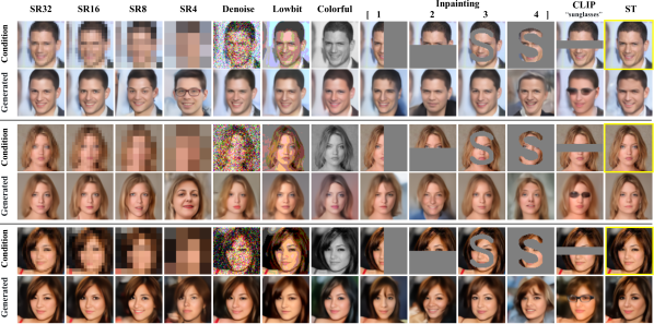
Most image generation models applied in daily life are conditional generative models. They generate corresponding images based on content provided by users, such as images to be edited , reference images [25], text descriptions, hand-drawn editing strokes [33], sketches, and so on. Current mainstream generative models [34, 24, 23] require training separate models and parameters for each condition. Each model has a fixed format for conditions and lacks an easy way to adjust the influence of each condition, limiting users’ creative possibilities. DDN support a wide range of zero-shot conditional generation, bringing more possibilities for user creativity. Fig. 2 demonstrates the capabilities of DDN in zero-shot conditional generation.

The core concept of Discrete Distribution Networks (DDN) is to approximate the distribution of training data using a multitude of discrete sample points. The secret to generating diverse samples lies in the network’s ability to concurrently generate multiple samples ($K$). This is perceived as the network outputting a discrete distribution – the origin of the name Discrete Distribution Networks. All generated samples serve as the sample space for this discrete distribution. Typically, each sample in this discrete distribution has an equal probability mass of $1/K$. Our goal is to make this discrete distribution as close as possible to the target dataset.

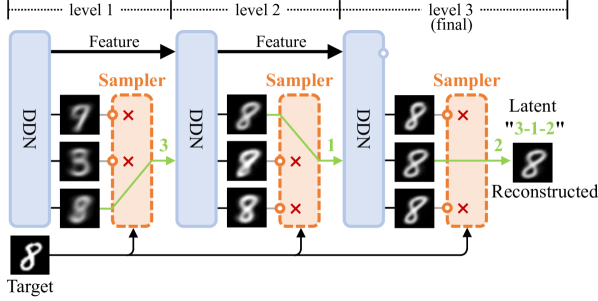
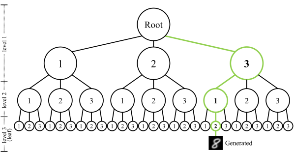
To accurately fit the target distribution of large datasets, a substantial representational space is required. In the most extreme scenario, this space must be larger than the number of training data samples. However, current neural networks lack the feasibility to generate such a vast number of samples simultaneously. Therefore, we adopt a strategy from autoregressive models [31] and partition this large space into a hierarchical conditional probability model. Each layer of this model needs only a small number of outputs. We then select one of these outputs as the output for that layer and use it as conditional input to the next layer. As a result, the output of the next layer will be more closely related to the selected conditional sample. If the number of layers is $L$ and the number of outputs per layer is $K$, then the output space of the network is $K^{L}$. Due to its exponential nature, this output space will be much larger than the number of samples in the dataset. Fig. 1 shows how DDN generates images.

We posit that the contributions of this paper are as follows:

• We introduce a novel generative model, termed Discrete Distribution Networks (DDN), which exhibit a more straightforward and streamlined principle and form.

• For training the DDN, we propose the “Split-and-Prune” optimization algorithm, and a range of practical techniques.

• We conduct preliminary experiments and analysis on the DDN, showcasing its intriguing properties and capabilities, such as zero-shot conditional generation and highly compact representations.

2 Related Work

Figure 3: Schematic of Discrete Distribution Networks (DDN). (a) The data flow during the training phase of DDN is shown at the top. As the network depth increases, the generated images become increasingly similar to the training images. Within each Discrete Distribution Layer (DDL), $K$ samples are generated, and the one closest to the training sample is selected as the generated image for loss computation. These $K$ output nodes are optimized using Adam with the Split-and-Prune method. The right two figures demonstrate the two model paradigms supported by DDN. (b) Single Shot Generator Paradigm: Each neural network layer and DDL has independent weights. (c) Recurrence Iteration Paradigm: All neural network layers and DDLs share weights. For inference, replacing the Guided Sampler in the DDL with a random choice enables the generation of new images.

Deep Generative Model. Generative Adversarial Networks (GANs) [21, 2] and Variational Autoencoders (VAEs) [16, 32] are two early successful generative models. GANs reduce the divergence between the generated sample distribution and the target distribution through a game between the generator and discriminator. However, regular GANs cannot map samples back to the latent space, thus they cannot reconstruct samples. VAEs encode data into a simple distribution’s latent space through an Encoder, and the Decoder is trained to reconstruct the original data from this simple distribution’s latent space. Notably, VQ-VAE [32], an important improvement of VAEs, achieves a more compact discrete representation by replacing the VAE’s latent space with discrete codebooks. However, this discrete representation still has a 2D structure, leading to a significant amount of redundant information. Moreover, VQ-VAE relies on a prior network to perform generative tasks. Autoregressive models [29] , with their simple principles and methods, model the target distribution by decomposing the target data into conditional probability distributions of each component. They can also compute the exact likelihood of target samples. However, the efficiency of these models is reduced when dealing with image data, which is not suitable to be decomposed into a sequence of components. Normalizing flow [14] is another class of generative models that can compute the likelihood. They use invertible networks to construct a mapping from samples to a noise space, and during the generation stage, they map back from noise to samples. Energy Based Models (EBM) [6, 28] with their high-quality and rich generative results, have led to the rise of diffusion models. However, their multi-step iterative generation process requires substantial computational resources.

Conditional image generation. Early conditional image generation methods were primarily dominated by GAN-based methods [10, 36, 19]. However, these methods require a considerable amount of paired condition-image data and necessitate training different models for distinct condition tasks. Recent works have demonstrated the excellent zero-shot conditional generation capacity of diffusion models [19, 18]. One approach is to add a moderate amount of noise to the image-based condition, ensuring that the condition’s structure is not completely destroyed by the noise, and making it quite similar to an image containing noise at a certain step in the diffusion training process. The denoising process of diffusion then yields realistic images. However, these diffusion-based zero-shot conditional generation methods cannot handle non-image-based conditions, such as generating samples of a specific category under the guidance of a classifier.

3 Discrete Distribution Networks

(a) Initial, K=5

(b) Split, K=5→6

(c) Prune, K=6→5

(d) Final, K=5

Figure 4: Illustration of the Split-and-Prune operation. For example in (a), the light blue bell-shaped curve represents a one-dimensional target distribution. The 5 “↑” under the x-axis are the initial values from a uniform distribution of 5 output nodes, which divide the entire space into 5 parts using midpoints between adjacent nodes as boundaries (i.e., vertical gray dashed lines). Each part corresponds to the range represented by this output node on the continuous space $x$. Below each node are three values: $P$ stands for the relative frequency of the ground truth falling within this node’s range during training; $Q$ refers to the probability mass of this sample (node) in the discrete distribution output by the model during the generation phase, which is generally equal for each sample, i.e., $1/K$. The bottom-most value denotes the difference between $P$ and $Q$. Colorful horizontal line segments represent the average probability density of $P$, $Q$ within corresponding intervals. In (b), the Split operation selects the node with the highest $P$ (circled in red). In (c), the Prune operation selects the node with the smallest $P$ (circled in red). In (d), through the combined effects of loss and Split-and-Prune operations, the distribution of output nodes moves towards final optimization. From the observed results, the KL divergence ($KL(P||Q)$) consistently decreases as the operation progresses, and the yellow line increasingly approximates the light blue target distribution.

3.1 Network Architecture

Fig. 3(a) illustrates the overall structure of the DDN, comprised of Neural Network Blocks and Discrete Distribution Layers (DDL). Each DDL contains $K$ output nodes, each of which is a set of 1x1 convolutions responsible for transforming the feature into the corresponding output image. The parameters of these 1x1 convolutions are optimized by Adam with Split-and-Prune. The $K$ images generated by the $K$ output nodes are inputted into the Guided Sampler. The Guided Sampler selects the image with the smallest L2 distance to the training image, which serves as the output of the current layer and is used to calculate the L2 loss with the training image. Simultaneously, the selected image is concatenated back into the feature, acting as the condition for the next block. The index (depicted in green as “K-1” in Fig. 3(a)) of the selected image represents the latent value of the training sample at this layer. Through the guidance of the Guided Sampler layer by layer, the image generated by the network progressively becomes more similar to the training sample until the final layer produces an approximation of the training sample. We average the L2 loss across each layer as the final loss of the entire network.

When the network performs the generation task, replacing the Guided Sampler with a random choice enables image generation. Given the exponential representational space of $K^{L}$ sample space and the limited number of samples in the training set, the probability of sampling an image with the same latent space as those in the training set is also exponentially low. For image reconstruction tasks, the process is almost identical to the training process, only substituting the training image with the target image to be reconstructed and omitting the L2 Loss part from the training process. The Final Generated Image in Fig. 3(a) represents the final reconstruction result. The indices of the selected samples along the way form the latent of the target image. Therefore, the DDN latent is a sequence of integers with length $L$, which we regard as the hierarchical discrete representation of the target sample. The latent space exhibits a tree structure with $L$ layers and $K$ degrees per node, where each leaf node represents a sample space, and its latent representation indicates the indices of all nodes along the path to this leaf node, as shown in Fig. 1(b). In the latent sequence, values placed earlier correspond to higher-level nodes in the tree, controlling the low-frequency information of the output sample, while later values tend to affect high-frequency information.

For computational efficiency, we adopted a decoder structure similar to the generator in GANs for coarse-to-fine image generation, as shown in Fig. 3(b). We refer to this as the Single Shot Generator. As each layer of DDN can naturally input and output RGB domain data, DDN seamlessly support the Recurrence Iteration Paradigm Fig. 3(c).

Figure 5: Toy examples for two-dimensional data generation. The numerical values at the bottom of each figure represent the Kullback-Leibler (KL) divergence. Due to phenomena such as “dead nodes” and “density shift”, the application of Gradient Descent alone fails to properly fit the Ground Truth (GT) density. However, by employing the Split-and-Prune strategy, the KL divergence is reduced to even lower than that of the Real Samples. More instructions for this experiment are in the Appendix.

3.2 Optimiztion with Split-and-Prune

We have observed two primary issues resulting from each layer calculating loss only with the closest output samples to the ground truth (GT). Firstly, a problem similar to the“dead codebooks” in VQ-VAE arises, wherein output nodes that are not selected for a long time receive no gradient updates. During generation, these “dead nodes” are selected with equal probability, leading to poor output. The second issue is the probability density shift. For instance, in a one-dimensional asymmetric bimodal distribution, the target distribution is a mixture of two thin and tall Gaussian distribution functions, with one larger and one smaller peak. The means of these two peaks are -1 and 1, respectively. Therefore, half of the output samples with initial values less than 0 will be matched with samples from the larger peak and optimized towards the larger Gaussian distribution. Meanwhile, the other half of the output samples with values greater than 0 will be optimized towards the smaller Gaussian. A problem arises as the large and small peaks carry different probability masses but occupy equal portions of the output samples, resulting in the same sampling probability during generation.

Algorithm 1 Split-and-Prune for Training

1:Output nodes number $K$, model $f$, non-output parameters $\boldsymbol{\theta}$, target distribution $q(\mathbf{x})$

2:Initialize output node parameters $\mathbf{\boldsymbol{\psi}}(k)$ for $k\in\{1,\dotsc,K\}$ with random values

3:Initialize counter $\mathbf{c}(k)=0$ for $k\in\{1,\dotsc,K\}$

4:Set split/prune threshold $P_{split}\leftarrow 2/K$, $P_{prune}\leftarrow 0.5/K$

5:$n\leftarrow 0$, $k_{new}\leftarrow K+1$

6:repeat

7:    $\mathbf{x}\sim q(\mathbf{x})$

8:    Choose $k^{*}=\underset{k}{\operatorname{argmin}}\;\left\|f(\boldsymbol{\theta},\boldsymbol{\psi}(k))-\mathbf{x}\right\|^{2}$

9:    Gradient descent $\nabla_{\boldsymbol{\theta},\boldsymbol{\psi}(k^{*})}\left\|f(\boldsymbol{\theta},\boldsymbol{\psi}(k^{*}))-\mathbf{x}\right\|^{2}$

10:    $\mathbf{c}(k^{*}):=\mathbf{c}(k^{*})+1$

11:    $n\leftarrow n+1$

12:    $k_{max}=\underset{k}{\operatorname{argmax}}\;\mathbf{c}(k)$ and $k_{min}=\underset{k}{\operatorname{argmin}}\;\mathbf{c}(k)$

13:    if  $\mathbf{c}(k_{max})/n>P_{split}$ or $\mathbf{c}(k_{min})/n<P_{prune}$ then

14:   # Split:

15:         $\mathbf{\boldsymbol{\psi}}(k_{new}):=\operatorname{clone}(\mathbf{\boldsymbol{\psi}}(k_{max}))$

16:         $\mathbf{c}(k_{new}):=\mathbf{c}(k_{max})/2$

17:         $\mathbf{c}(k_{max}):=\mathbf{c}(k_{max})/2$

18:         $k_{new}\leftarrow k_{new}+1$

19:   # Prune:

20:         $n\leftarrow n-\mathbf{c}(k_{min})$

21:         $\operatorname{remove}\;\mathbf{\boldsymbol{\psi}}(k_{min})$ and $\mathbf{c}(k_{min})$

22:    end if

23:until converged

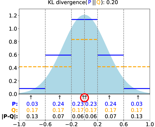
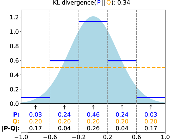
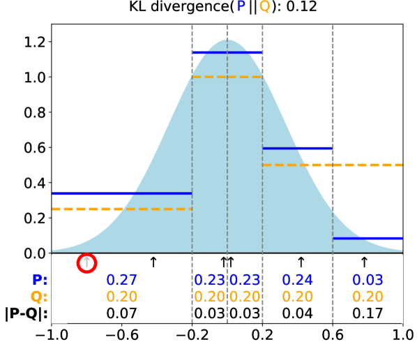
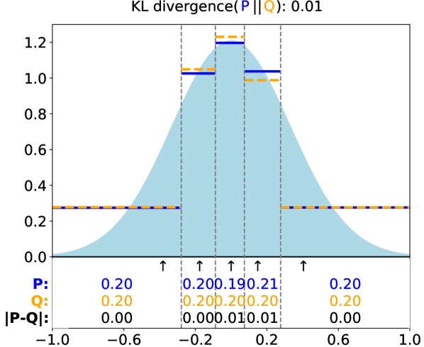
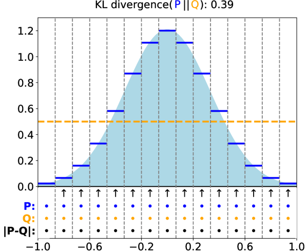
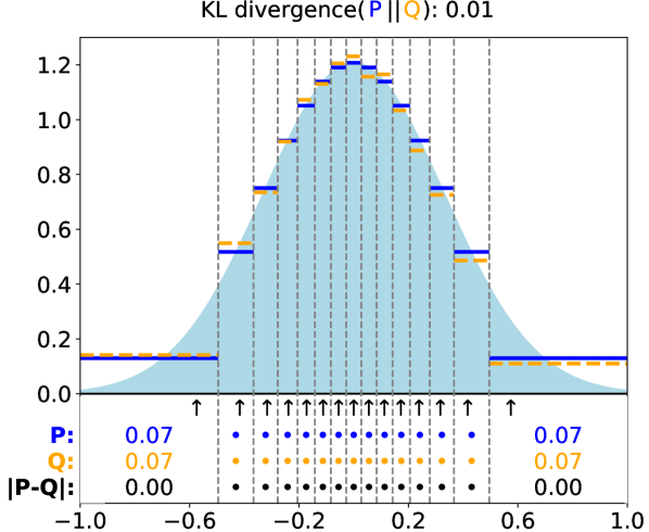
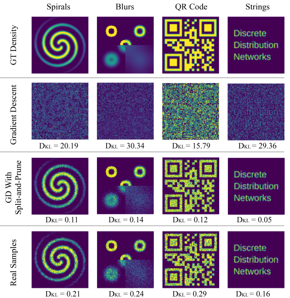
Inspired by the theory of evolution, we propose a new optimization algorithm—Split-and-Prune—to address the above issues, as outlined in Algorithm 1. The Split operation targets nodes frequently matched by training samples, while the Prune operation addresses the issue of “dead nodes”. These nodes are akin to species in evolution, subject to diversification and extinction. During training, we track the frequency with which each node is matched by training samples. For nodes with excessive frequency, we execute the Split operation, cloning the node into two new nodes, each inheriting half of the old node’s frequency. Although these two new nodes have identical parameters and outputs, the next matched training sample will only be associated with one node. Therefore, the loss and gradient only affect one node’s parameters. Consequently, their parameters and outputs exhibit slight differences, dividing the old node’s match space into two. In subsequent training, the outputs of the two new nodes will move towards the centers of their respective spaces under the influence of the loss, diverging to produce more diverse outputs. For nodes with low matching frequency (dead nodes), we implement the Prune operation, removing them outright. Fig. 4 illustrates the process of the Split-and-Prune operation and how it reduces the distance between the discrete distribution represented by the Output Nodes and the target distribution. The efficacy of the Split-and-Prune optimization algorithm is validated through examples of fitting 2d density maps in Fig. 5.

3.3 Applications

Zero-Shot Conditional Generation (ZSCG). Each layer of the DDN produces multiple target samples, with a selected sample being forwarded as a condition to the next layer. This enables the generation of new samples in the desired direction, ultimately producing a sample that meets the given condition. Indeed, the reconstruction process shown in Fig. 1(a) is a ZSCG process guided by a target image, which never directly enters the network.

To implement ZSCG, we replace the Guided Sampler in Fig. 3(a) with a Conditional Guided Sampler. For instance, when generating an image of class $y_{i}$ guided by a classifier, we replace the “L2 Distance to Training Image” in the Guided Sampler of Fig. 3(a) with the probability of each output image belonging to class $y_{i}$ according to the classifier. We then replace “argmin” with “argmax” to construct the Guided Sampler for this classifier.

For super-resolution and colorization tasks, we construct a transform that converts the generated images to the target domain (low-resolution or grayscale images). This approach significantly reduces the impact of the missing signal from the condition on the generated images, enabling DDN to perform even very low-resolution super-resolution tasks.

The use of “argmax” in the Guided Sampler causes each layer to select a fixed sample, resulting in a single image output for each condition, similar to the Greedy Sampling in GPT. To increase diversity, we employ more flexible sampling methods. For most ZSCG tasks, we use Top-k sampling with $k=2$, balancing diversity and condition appropriateness in the large generation space ($2^{L}$).

The versatility of ZSCG can be further enhanced by combining different Guided Samplers. For example, an image can guide the primary structure while text guides the attributes. The influence of each condition can be adjusted by setting their respective weights. Experiments involving the combination of different Guided Samplers will be presented in the Appendix.

Efficient Data Compression Capability. The latent of DDN is a highly compressed discrete representation, where the information content of a DDN latent is $L\times\log_{2}{K}$ bits. Taking our default experimental values of $K$=512 and $L$=128 as an example, a sample can be compressed to 1152 bits, demonstrating the efficient lossy compression capability of DDN. We hypothesize this ability originates from two aspects: 1) the compact hierarchical discrete representation, and 2) the Split-and-Prune operation makes the probabilities of each node as equal as possible, thereby increasing the information entropy [26] of the entire latent distribution and more effectively utilising each bit within the latent.

In our experiments, we set $K$=512 as the default, considering the balance between generation performance and training efficiency. However, from the perspective of data compression, setting $K$ to 2 and increasing $L$ provides a better balance between representation space and compression efficiency. We refer to DDN with $K$=2 as Binary DDN (BinDDN). To the best of our knowledge, BinDDN are the first generative model capable of directly transforming data into semantically meaningful binary strings. These binary strings represent a leaf node on a balanced binary tree.

3.4 Techniques

In this subsection, we present several techniques for training Discrete Distribution Networks.

Chain Dropout. In scenarios where the number of training samples is limited, each data sample undergoes multiple training iterations within the network. During these iterations, similar selections are often made by the Guided Sampler at each layer. However, the representational space of DDN far exceeds the number of training samples in the dataset. This disparity leads to a situation where the network is only trained on a very limited set of pathways, resulting in what can be perceived as overfitting on these pathways. To mitigate this, we introduce a strategy during training where each Discrete Distribution Layer substitutes the Guided Sampler with a “random choice” at a fixed probability rate. We refer to this method as “Chain Dropout”.

Learning Residual. In the context of utilizing the Single Shot Generator structure, a Discrete Distribution Layer is introduced every two convolution layers. Given such small amount of computation between adjacent layers, directly regressing the images themselves with these convolutions becomes challenging. Drawing inspiration from ResNet [8], we propose a scheme for the network to learn the residual between the output images from the preceding layer and the ground truth. The output of the current layer is then computed as the sum of the output from the previous layer and the current layer’s residual. This approach alleviates the pressure of the network to represent complex data and enhances the flexibility of the network.

Leak Choice. In each layer of the DDN, the output is conditioned on the image selected from the previous layer. This condition serves as a signal in the image domain, requiring the current layer to expend computational resources to extract features and interpret the choices made by the Sampler. However, for a DDN with a Single Shot Generator structure, the computation between two adjacent layers is minimal, involving only two convolutional layers. To facilitate faster understanding of the choices made by the Sampler in the subsequent layer, we have added extra convolutional layers to each output node. The features produced by these extra convolutions also serve as conditional inputs to the next layer. But these features don’t participate in the calculation of distance or loss in DDL.

(a) CelebA-HQ 64x64

(b) FFHQ 64x64

(c) CIFAR

(d) Conditional CIFAR

(e) Conditional MNIST

Figure 6: Random samples from DDN. Figures (d) and (e) showcase images that are conditionally generated by conditional DDN, with each row of images representing a distinct category.

4 Experiments

Method	Type	One-Step Generation	FID↓
DCGAN[21]	GAN	✓	37.1
BigGAN[2]	GAN	✓	14.1
IGEBM[6]	EBM	✗	38.0
Denoising Diffusion[28]	EBM	✗	3.2
VAE[16]	VAE	✓	106.7
Gated PixelCNN[29]	AR	✗	65.9
GLOW[14]	Flow	✓	46.0
DDN(ours)	DDN	✓	52.0

Table 1: Quantitative comparison on CIFAR-10

Figure 7: Zero-Shot Conditional Generation on CIFAR-10 Guided by a Pretrained Classification Model. Each row corresponds to a class in CIFAR-10. Specifically, the first row consists of airplanes, the third row displays birds flying against the blue sky, and the last row presents trucks. Our model successfully generates reasonable images for each class without any conditional training, demonstrating the powerful zero-shot generation capability of our DDN.

Model	FID↓	rFID-FFHQ↓	rFID-CelebA↓
K=512 (default)	43.1	26.0	33.2
K=64	47.0	32.3	38.7
K=8	52.6	40.9	49.8
K=2 (BinDDN)	66.5	38.4	70.6
w/o Split-and-Prune	55.3	31.2	34.7
w/o Chain Dropout	182.3	26.5	37.4
w/o Learning Residual	56.2	40.2	40.2
w/o Leak Choice	56.0	34.3	32.2

Table 2: Ablation study on FFHQ-64x64. We use the reconstruction Fréchet Inception Distance (rFID) to reflect the reconstructive performance of the network. All models are trained on the FFHQ-64x64 dataset. The rFID-FFHQ represents the reconstructive performance of the model on the training set, while rFID-CelebA can be seen as an indication of the model’s generalization performance on the test set. “w/o” stands for “without”.

We trained our models on a server equipped with 8 RTX2080Ti GPUs, setting the Chain Dropout probability to 0.05 by default. For the 64x64 resolution experiments, we utilized a DDN with 93M parameters, setting $K=512$ and $L=128$. In the CIFAR experiments, we employed a DDN with 74M parameters, setting $K=64$ and $L=64$. The MNIST experiments were conducted using a Recurrence Iteration Paradigm UNet model with 407K parameters, where $K=64$ and $L=10$. More extended experiments exploring the properties of DDN can be found in the Appendix.

4.1 Qualitative and Quantitative Results

Generation Quality. Fig. 6(a) and Fig. 6(b) depict random generation results of DDN on CelebA-HQ-64x64 [12] and FFHQ-64x64 [13], verifying the model’s effectiveness in modeling facial data. The generation quality on CelebA-HQ appears superior to that on FFHQ, which is also reflected in the lower FID score (35.4 VS 43.1). We surmise this disparity arises from CelebA-HQ’s relatively cleaner backgrounds and less diverse facial data compared to FFHQ.

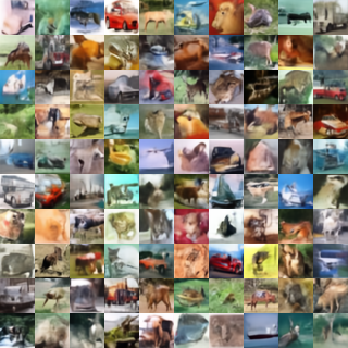
Fig. 6(c) demonstrates the random generation results of DDN on CIFAR. Concurrently, we report the FID score of DDN on Unconditional CIFAR in Tab. 1, comparing it with classical methods of other generative models. The FID of DDN surpasses that of VAE [15] and Gated PixelCNN [30].

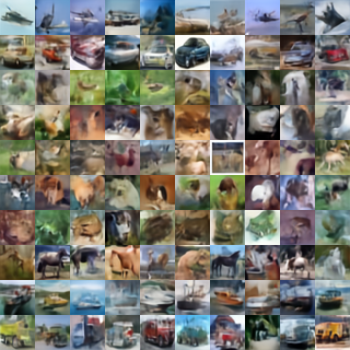
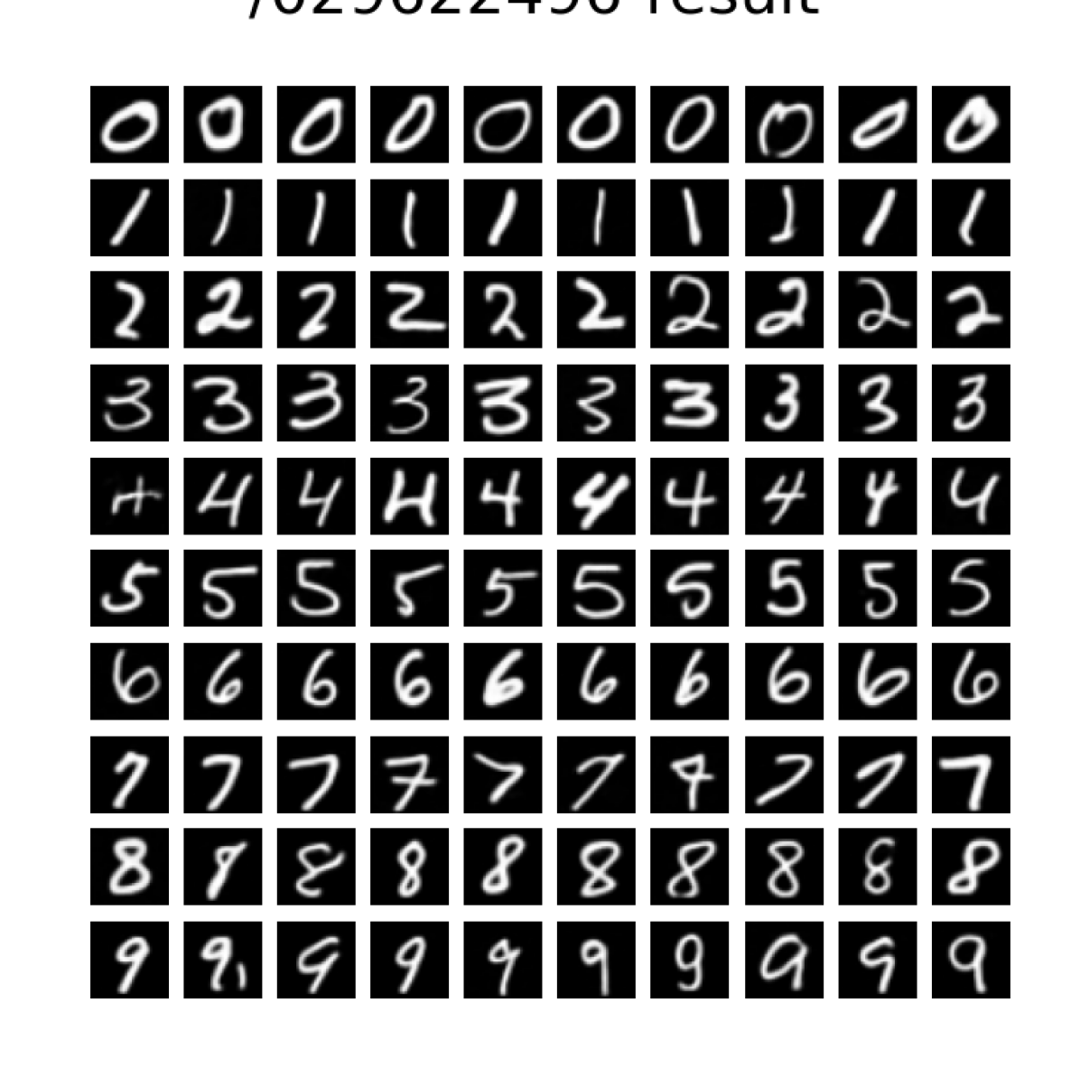
Training a conditional DDN is quite straightforward, it only requires the input of the condition or features of the condition into the network, and the network will automatically learn $P(X|Y)$. Fig. 6(d) and Fig. 6(e) show the generation results of the class-conditional DDN on CIFAR and MNIST, respectively. The conditional DDN displays a strong ability to learn the correct $P(X|Y)$ distribution.

Zero-Shot Conditional Generation. We trained a DDN model on the FFHQ-64x64 dataset and then tested the capability of the model for zero-shot conditional image generation using the CelebA-HQ-64x64 dataset, as shown in Fig. 2. We presented the experiments of text-guided ZSCG using CLIP [22] in the Appendix. Our generation process does not require gradient derivation or numerical optimization, nor does it need iterative steps.

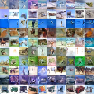
In addition, we employed an off-the-shelf CIFAR classifier [20] to guide the generation of specific category images by a DDN model trained unconditionally on CIFAR. We want to emphasize that the classifier is an open-source, pre-trained ResNet18 model, with no additional modifications or retraining. Fig. 7 displays images of various CIFAR categories generated by the model under the guidance of the classifier.

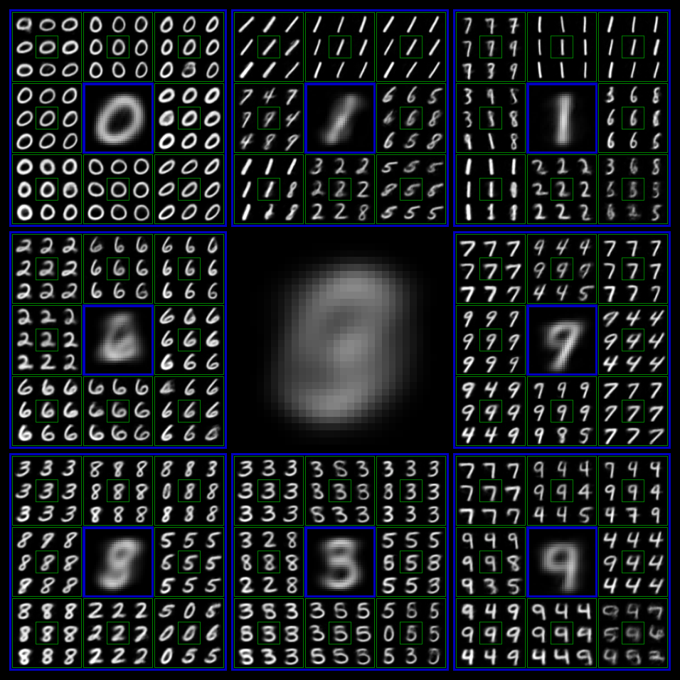
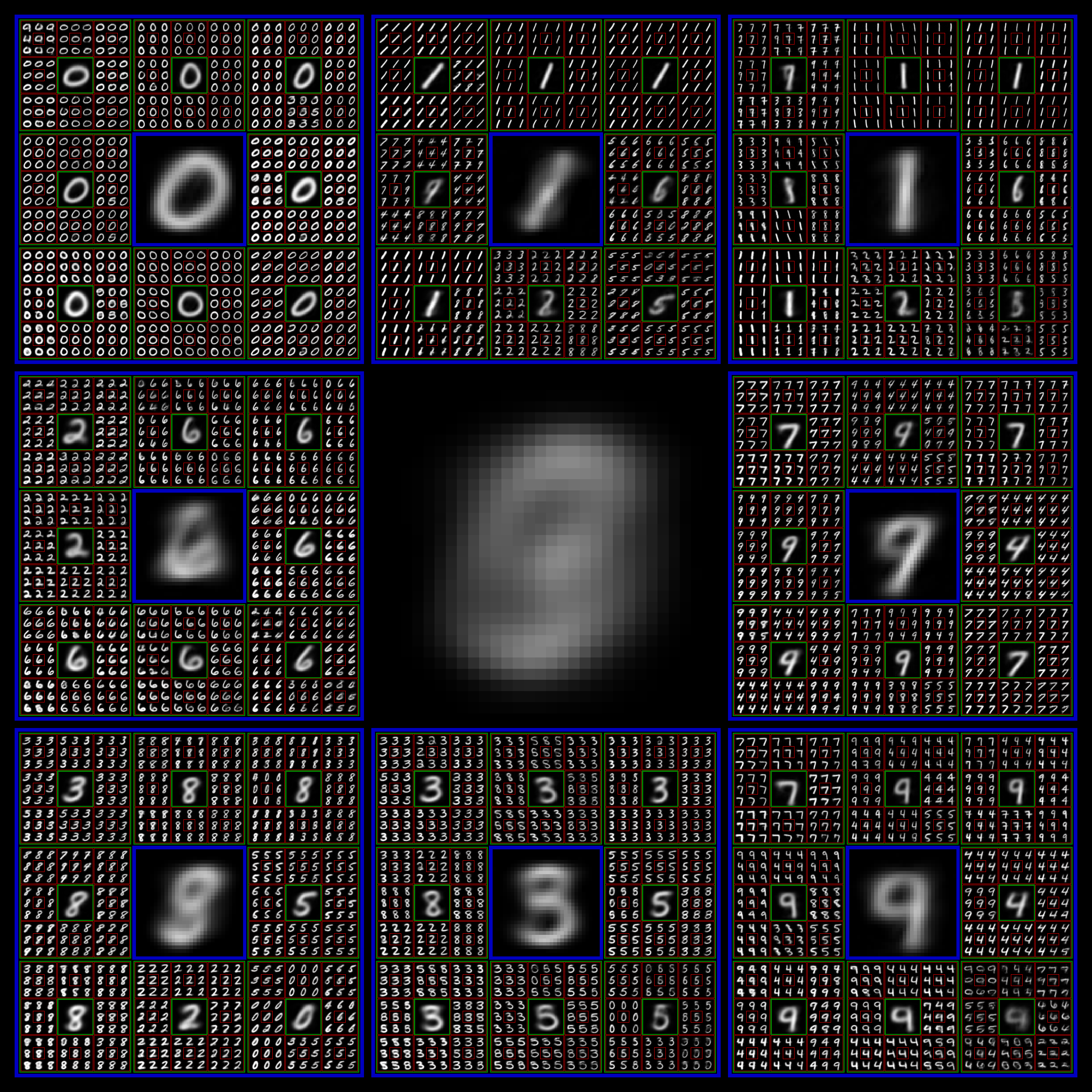
Latent analysis. We trained a DDN on the MNIST dataset with $K=8$ and $L=3$ to visualize both the hierarchical generative behavior of the DDN and the distribution of samples in the entire latent representation space, as shown in Figure 8.

Figure 8: Hierarchical Generation Visualization of DDN. We trained a DDN with output level $L=3$ and output nodes $K=8$ per level on MNIST dataset, its latent hierarchical structure is visualized as recursive grids. Each sample with a colored border represents an intermediate generation product. The samples within the surrounding grid of each colored-bordered sample are refined versions generated conditionally based on it (enclosed by the same color frontier). The small samples without colored borders are the final generated images. The larger the image, the earlier it is in the generation process, implying a coarse version. The large image in the middle is the average of all the generated images. More detailed visualization of $L=4$ will be presented in the Appendix.

4.2 Ablation Study

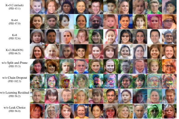
In Table 2, we demonstrate the impact of different numbers of output nodes ($K$) and various techniques on the network. Interestingly, despite the substantial difference between having and not having the Split-and-Prune technique in the toy example, as shown in Figure 5, the performance in the ablation study without Split-and-Prune is not as poor as one might expect. We hypothesize that this is due to the Chain Dropout forcing all dead nodes to receive gradient guidance, preventing the network from generating poor results that are unoptimized. A particular case is when $K=2$, where the representational space of BinDDN is already sufficiently compact. The use of Chain Dropout in this case tends to result in more blurred generated images. Therefore, we did not employ Chain Dropout when $K=2$.

5 Conclusion

In this paper, we have introduced Discrete Distribution Networks, a generative model that approximates the distribution of training data using an multitude of discrete sample points. DDN exhibit two intriguing properties: they support more general zero-shot conditional generation and offer highly compressed representation. Additionally, we proposed the Split-and-Prune optimization algorithm and several effective techniques for training DDN.

Acknowledgements. Special thanks to Haikun Zhang for her comprehensive support, including but not limited to paper formatting, CIFAR classification experiments. Thanks to Yihan Xie for her significant assistance in illustrations and CLIP experiments. Gratitude is extended to Jiajun Liang and Haoqiang Fan for helpful discussions. Thanks to Xiangyu Zhang for hosting the Generative Model Special Interest Group. Appreciation is also given to Hung-yi Lee for developing and offering his engaging machine learning course.

Supplementary Material

6 Further Demonstrations on Zero-Shot Conditional Generation

In this section, we present additional experimental results on Zero-Shot Conditional Generation (ZSCG).

Figure 9: Zero-Shot Conditional Generation guided by CLIP. The text at the top is the guide text for that column.

Figure 10: Zero-Shot Conditional Generation under the Influence of Multiple Conditions. The DDN balances the steering forces of CLIP and Inpainting according to their associated weights.

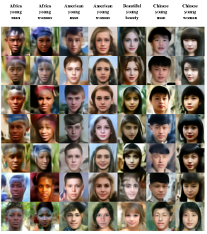
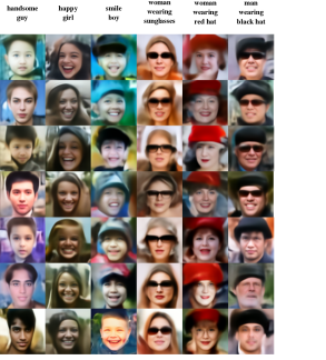
Utilizing CLIP as Conditioning Guidance. As illustrated in Fig. 9, we leverage CLIP [22] along with corresponding prompts as conditioning cues. We use a Discrete Distribution Network (DDN) model, which is exclusively trained on the FFHQ dataset, to yield Zero-Shot Conditional Generation (ZSCG) results. Remarkably, DDN can generate corresponding images under the guidance of CLIP without the necessity for gradient computations and only requiring a single inference pass.

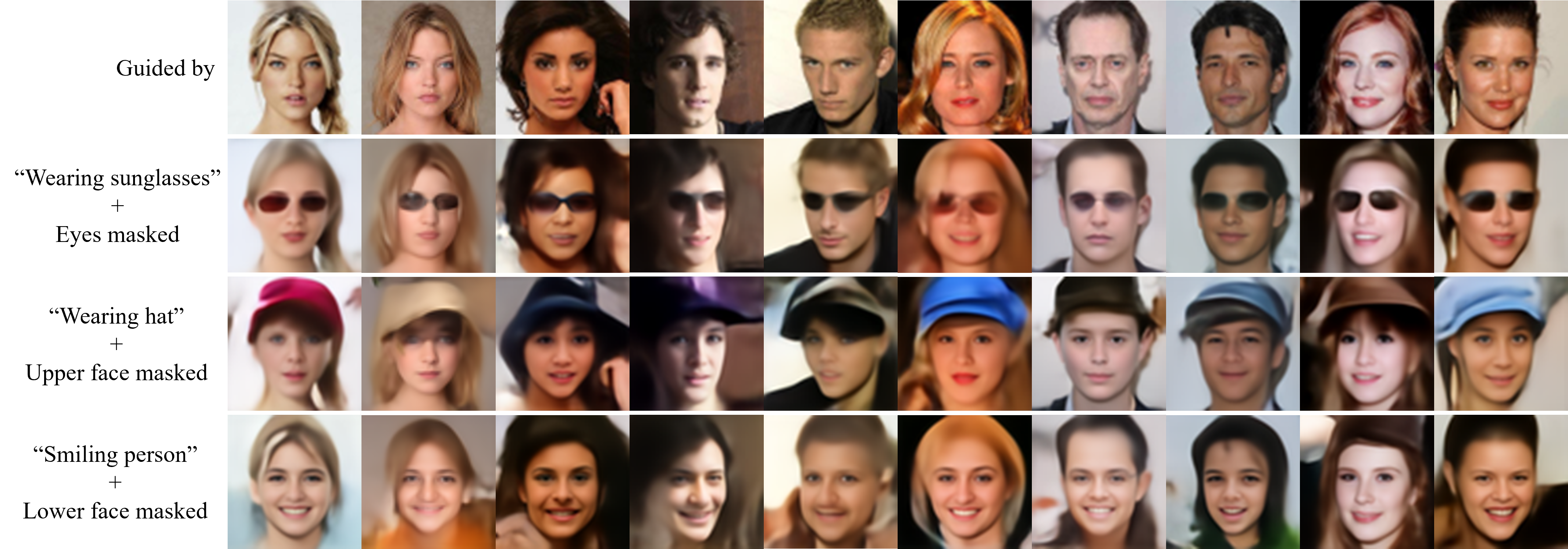
ZSCG with Multiple Conditions. In Fig. 10, we illustrate the operation of ZSCG under the combined action of two Guided Samplers: Inpainting and CLIP. Each sampler operates under its own specific condition. The inpainting sampler utilizes a mask to cover the areas where the CLIP prompt acts. Specifically, “wearing sunglasses” masks the eyes, “wearing a hat” masks the upper half of the face, and “happy person” masks the lower half. For each Discrete Distribution Layer (DDL), both samplers assign a rank to the generated images, corresponding to the degree of match to their respective conditions– the better the match, the higher the rank. We assign a weight to each sampler, which affects the assigned ranking. In this case, both samplers have a weight of 0.5. To promote diversity in the generated samples, we randomly select one image from the top two ranked by their condition-matching scores, serving as the output for that DDL layer.

Supplementary ZSCG Experimental Data. We have provided raw experimental data in the zip file of the Supplementary Material. These data have not been filtered nor have we applied any Reject Sampling strategy, hence there exist bad cases in certain ZSCG tasks such as facial recognition and CLIP-guided image editing. Notwithstanding, we emphasize that to the best of our knowledge, DDN is the first generative model capable of performing ZSCG tasks with non-image-based conditions without the need for gradients and iterations. The unprocessed data serve primarily to illustrate how DDN can effectively steer towards the correct direction under the guidance of non-image-based conditions.

7 Experimental Results on Generative Performance

We present additional experiments to verify the generative and reconstructive capabilities of Discrete Distribution Networks (DDN).

Verify whether DDN can generate new images. As depicted in Figure Fig. 11, we compare the images that are closest in the training dataset, FFHQ, to those generated by our DDNs. It suggests that our DDNs can synthesize new images that, while not present in the original dataset, still conform to its target distribution.

Figure 11: Nearest neighbors of the model trained on FFHQ. The leftmost column presents images generated by the DDN. Starting from the second column, we display the images from FFHQ that are most similar to the generated images, as measured by LPIPS [35].

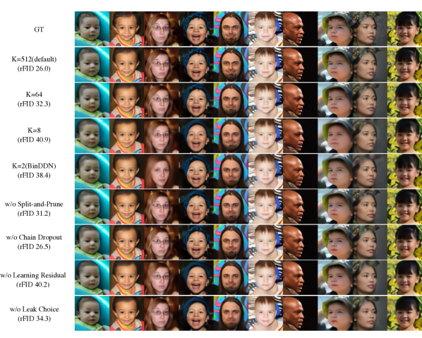
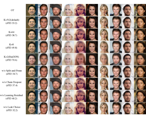
Demonstration of Generation and Reconstruction Quality. Figs. 13, 14 and 15 illustrate the generation and reconstruction results in various ablation experiments using the DDN model.

(a) With Split-and-Prune, Chain Dropout 0

(b) Without Split-and-Prune, Chain Dropout 0

(c) Without Split-and-Prune, Chain Dropout 0.05

Figure 12: Efficacy of Split-and-Prune and Chain Dropout on MNIST.

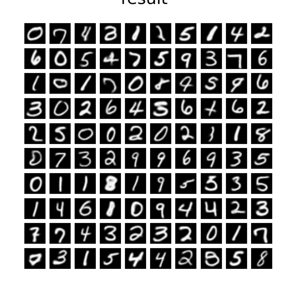
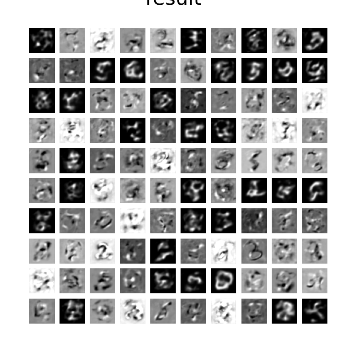
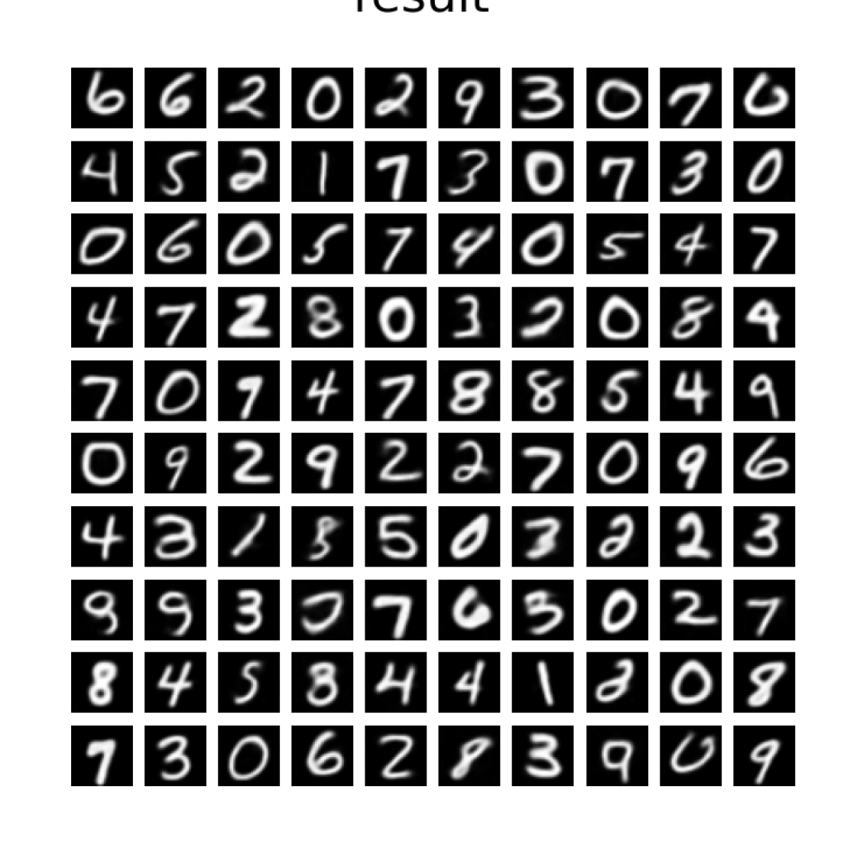
Efficacy of Split-and-Prune and Chain Dropout. A series of experiments were conducted to separately investigate the effectiveness of the Split-and-Prune and Chain Dropout methods. To isolate the impacts of these two algorithms, we simplified the experimental conditions as much as possible, using the MNIST dataset as a base, setting $K=8$ and $L=10$, and disabling Learning Residual. The generated image quality under three different settings is displayed in Fig. 12. The results demonstrated that the Split-and-Prune method is indispensable, leading to significant improvements in the quality of generated images. Meanwhile, the Chain Dropout method was found to alleviate the poor results observed when the Split-and-Prune method was not implemented.

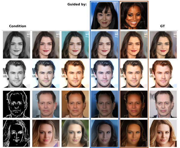
Conditional DDN for Image-to-Image Tasks. In the realm of image-to-image tasks, we extend our Discrete Distribution Networks (DDN) to a conditional setting, resulting in the conditional DDN. In this architecture, the condition is directly fed into the network during training in the beginning of each stage. The condition serves as an informative guide, significantly reducing the model’s generative space and, consequently, the complexity of the modeling task.

Those conditions inherently carry rich information, enabling the network to produce higher-quality samples. Through this conditional design, the DDN can leverage the abundant information contained in the conditions to generate more accurate and detailed images as shown in Fig. 16.

Figure 13: Illustration of the random sample generation effects as part of the ablation study on our DDNs model.

Figure 14: Demonstration of the reconstruction capability of our ablation study model on FFHQ-64x64, which can be interpreted as the model’s fitting ability on the training set.

Figure 15: Demonstration of the reconstruction capability of our ablation study model on CelebA-64x64, which can be interpreted as the model’s generalization ability on the test set.

Figure 16: Conditional DDN performing coloring and edge-to-RGB tasks. Columns 4 and 5 display the generated results under the guidance of other images, where the produced image strives to adhere to the style of the guided image as closely as possible while ensuring compliance with the condition. The resolution of the generated images is $256\times 256$.

8 Latent Analysis

Nodes/level	Level	Representation space	Validation accuracy↑
$\mathrm{K}$	$\mathrm{L}$	$\mathrm{K}^{\mathrm{L}}$	128	1024	10k	50k
2	10	1024	65.9	77.3	85.8	86.9
8	3	512	69.0	81.1	87.6	88.0
8	5	$3.3\text{\times}{10}^{4}$	67.5	79.1	87.5	90.5
8	10	$1.1\text{\times}{10}^{9}$	58.6	75.3	84.9	89.0
64	10	$1.1\text{\times}{10}^{18}$	52.5	70.4	80.9	86.3

Table 3: Fine-tuning DDN latent as decision tree on MNIST. Constructing a decision tree based on the latent variables from the DDN and fine-tuning it on MNIST trainning set. We report the validation set accuracy of the decision tree after majority voting for class prediction with varying number of training samples: 128, 1,024, 10,000, and 50,000 (the full training set).

Semantic Performance of Latents. We explored the semantic capabilities of DDN latents through a classification experiment on the MNIST dataset. Given the inherent tree structure of DDN’s latents, we employed a decision tree classification method, using fine-tuning data to assign class votes to nodes in the tree. For unassigned nodes, their class is inherited from the closest ancestor node with a class. We fine-tuned DDN’s latent decision tree using various numbers of labeled training set data, and the results on the test set are shown in Tab. 3. All experiments in this table were conducted with Recurrence Iteration Paradigm’s UNet, which has approximately 407k parameters. However, computational complexity increases proportionally with the number of output levels (L). These experiments substantiate that DDN’s latents encompass meaningful semantic information.

More Comprehensive Latent Visualization. Fig. 17 demonstrates a more comprehensive distribution of samples that correspond to the latent variables.

Figure 17: Hierarchical Generation Visualization of DDN with $L=4$. We trained a DDN with output level $L=4$ and output nodes $K=8$ per level on MNIST dataset, its latent hierarchical structure is visualized as recursive grids. Each sample with a colored border represents an intermediate generation product. The samples within the surrounding grid of each colored-bordered sample are refined versions generated conditionally based on it (enclosed by the same color frontier). The small samples without colored borders are the final generated images. The larger the image, the earlier it is in the generation process, implying a coarse version. The large image in the middle is the average of all the generated images. The samples with blue borders represent the $8$ outputs of the first level, while those with green borders represent the $8^{2}=64$ outputs of the second level. It can be observed that images within the same grid display higher similarity, due to their shared “ancestors”. Best view in color and zoom in.

9 More detailed experimental explanation

In Fig. 18, we have expanded the “Illustration of the Split-and-Prune operation” by providing a schematic when $K$ increases to 15. This demonstrates that having a larger sample space results in an approximation that is closer to the target distribution.

In the caption of Fig. 19, we have detailed the experimental parameters for “Toy examples for two-dimensional data generation”. Additionally, we will explain why the KL divergence in our model is lower than that found in the Real Samples.

(a) Initial, K=5

(b) Split, K=5→6

(c) Prune, K=6→5

(d) Final, K=5

(e) Initial, K=15

(f) Final, K=15

Figure 18: Illustration of the Split-and-Prune operation. For example in (a), the light blue bell-shaped curve represents a one-dimensional target distribution. The 5 “↑” under the x-axis are the initial values from a uniform distribution of 5 output nodes, which divide the entire space into 5 parts using midpoints between adjacent nodes as boundaries (i.e., vertical gray dashed lines). Each part corresponds to the range represented by this output node on the continuous space $x$. Below each node are three values: $P$ stands for the relative frequency of the ground truth falling within this node’s range during training; $Q$ refers to the probability mass of this sample (node) in the discrete distribution output by the model during the generation phase, which is generally equal for each sample, i.e., $1/K$. The bottom-most value denotes the difference between $P$ and $Q$. Colorful horizontal line segments represent the average probability density of $P$, $Q$ within corresponding intervals. In (b), the Split operation selects the node with the highest $P$ (circled in red). In (c), the Prune operation selects the node with the smallest $P$ (circled in red). In (d), through the combined effects of loss and Split-and-Prune operations, the distribution of output nodes moves towards final optimization. From the observed results, the KL divergence ($KL(P||Q)$) consistently decreases as the operation progresses, and the yellow line increasingly approximates the light blue target distribution. Finally, we show the distributions of the initial and final stages when the number of output nodes $K=15$ in (e) and (f). Due to the increased representational space (higher resolution), in (f), the probability density distribution $Q$ (yellow line segment) is closer to the lightblue target distribution than in the case of $K=5$.

Figure 19: Toy examples for two-dimensional data generation. The numerical values at the bottom of each figure represent the Kullback-Leibler (KL) divergence. Due to phenomena such as “dead nodes” and “density shift”, the application of Gradient Descent alone fails to properly fit the Ground Truth (GT) density. By employing the Split-and-Prune strategy, the density map looks the same as Real Samples. In the experiment, we use $K=10,000$ discrete nodes to emulate the probability distribution of GT density. Each node encompasses two parameters, $x$ and $y$, initialized from a uniform distribution. Each experiment consists of 100,000 iterations, where in each iteration an L2 loss is calculated based only on the node closest to the GT. The GT density map is converted into a discrete distribution with bins of size $100\times 100$, which is then used to calculate the KL divergence against the discrete distribution represented by these nodes. The KL divergence of Split-and-Prune is even lower than that of the Real Samples. This is because our algorithm has been exposed to 100,000 sets of GT data, thus it better reflects the GT distribution compared to the ‘Real Samples’, which are drawn only 10,000 times from the GT distribution.

10 Limitations

Limitations. There are two key limitations of Discrete Distribution Networks (DDNs):

• Loss of high-frequency signals: The high level of data compression and the use of pixel L2 loss during optimization may result in the loss of high-frequency signals, causing the images to appear blurred. A potential improvement could be learning from VQ-GAN [5] and incorporating adversarial loss [4] to enhance the modeling of high-frequency signals.

• Difficulty with complex data: While random choice can generate decent facial data, DDNs struggle with complex data, such as ImageNet [17]. One possible solution is to learn an additional prior model dedicated to sampling output nodes.

References

- Bond-Taylor et al. [2021] Sam Bond-Taylor, Adam Leach, Yang Long, and Chris G Willcocks. Deep generative modelling: A comparative review of vaes, gans, normalizing flows, energy-based and autoregressive models. IEEE transactions on pattern analysis and machine intelligence, 2021.
- Brock et al. [2019] Andrew Brock, Jeff Donahue, and Karen Simonyan. Large Scale GAN Training for High Fidelity Natural Image Synthesis. arXiv:1809.11096, 2019.
- Brown et al. [2020] Tom B Brown, Benjamin Mann, Nick Ryder, Melanie Subbiah, Jared Kaplan, Prafulla Dhariwal, Arvind Neelakantan, Pranav Shyam, Girish Sastry, Amanda Askell, et al. Language models are few-shot learners. arXiv preprint arXiv:2005.14165, 2020.
- Creswell et al. [2018] Antonia Creswell, Tom White, Vincent Dumoulin, Kai Arulkumaran, Biswa Sengupta, and Anil A Bharath. Generative adversarial networks: An overview. IEEE signal processing magazine, 35(1):53–65, 2018.
- Esser et al. [2021] Patrick Esser, Robin Rombach, and Björn Ommer. Taming Transformers for High-Resolution Image Synthesis. arXiv:2012.09841, 2021.
- Goyal et al. [2021] Kartik Goyal, Chris Dyer, and Taylor Berg-Kirkpatrick. Exposing the Implicit Energy Networks behind Masked Language Models via Metropolis–Hastings. arXiv:2106.02736, 2021.
- Graves et al. [2023] Alex Graves, Rupesh Kumar Srivastava, Timothy Atkinson, and Faustino Gomez. Bayesian flow networks. arXiv preprint arXiv:2308.07037, 2023.
- He et al. [2016] Kaiming He, Xiangyu Zhang, Shaoqing Ren, and Jian Sun. Deep Residual Learning for Image Recognition. In IEEE CVPR, 2016.
- Ho et al. [2020] Jonathan Ho, Ajay Jain, and Pieter Abbeel. Denoising diffusion probabilistic models, 2020.
- Isola et al. [2017] Phillip Isola, Jun-Yan Zhu, Tinghui Zhou, and Alexei A Efros. Image-to-image translation with conditional adversarial networks. In Proceedings of the IEEE conference on computer vision and pattern recognition, pages 1125–1134, 2017.
- Johnson et al. [2016] Justin Johnson, Alexandre Alahi, and Li Fei-Fei. Perceptual losses for real-time style transfer and super-resolution. In Computer Vision–ECCV 2016: 14th European Conference, Amsterdam, The Netherlands, October 11-14, 2016, Proceedings, Part II 14, pages 694–711. Springer, 2016.
- Karras et al. [2017] Tero Karras, Timo Aila, Samuli Laine, and Jaakko Lehtinen. Progressive growing of gans for improved quality, stability, and variation. arXiv preprint arXiv:1710.10196, 2017.
- Karras et al. [2019] Tero Karras, Samuli Laine, and Timo Aila. A style-based generator architecture for generative adversarial networks. In Proceedings of the IEEE/CVF conference on computer vision and pattern recognition, pages 4401–4410, 2019.
- Kingma and Dhariwal [2018] Durk P Kingma and Prafulla Dhariwal. Glow: Generative Flow with Invertible 1x1 Convolutions. NeurIPS 31, 2018.
- Kingma and Welling [2013] Diederik P Kingma and Max Welling. Auto-encoding variational bayes. arXiv preprint arXiv:1312.6114, 2013.
- Kingma and Welling [2014] Diederik P. Kingma and Max Welling. Auto-Encoding Variational Bayes. ICLR, 2014.
- Krizhevsky et al. [2012] Alex Krizhevsky, Ilya Sutskever, and Geoffrey E Hinton. Imagenet classification with deep convolutional neural networks. Advances in neural information processing systems, 25, 2012.
- Lugmayr et al. [2022] Andreas Lugmayr, Martin Danelljan, Andres Romero, Fisher Yu, Radu Timofte, and Luc Van Gool. Repaint: Inpainting using denoising diffusion probabilistic models. In Proceedings of the IEEE/CVF Conference on Computer Vision and Pattern Recognition, pages 11461–11471, 2022.
- Meng et al. [2021] Chenlin Meng, Yutong He, Yang Song, Jiaming Song, Jiajun Wu, Jun-Yan Zhu, and Stefano Ermon. Sdedit: Guided image synthesis and editing with stochastic differential equations. arXiv preprint arXiv:2108.01073, 2021.
- Phan [2021] Huy Phan. github.com/huyvnphan/PyTorch_CIFAR10, 2021.
- Radford et al. [2016] Alec Radford, Luke Metz, and Soumith Chintala. Unsupervised Representation Learning with Deep Convolutional Generative Adversarial Networks. In ICLR, 2016.
- Radford et al. [2021] Alec Radford, Jong Wook Kim, Chris Hallacy, Aditya Ramesh, Gabriel Goh, Sandhini Agarwal, Girish Sastry, Amanda Askell, Pamela Mishkin, Jack Clark, et al. Learning transferable visual models from natural language supervision. In International conference on machine learning, pages 8748–8763. PMLR, 2021.
- Ramesh et al. [2022] Aditya Ramesh, Prafulla Dhariwal, Alex Nichol, Casey Chu, and Mark Chen. Hierarchical text-conditional image generation with clip latents. ArXiv, abs/2204.06125, 2022.
- Rombach et al. [2021] Robin Rombach, A. Blattmann, Dominik Lorenz, Patrick Esser, and Björn Ommer. High-resolution image synthesis with latent diffusion models. 2022 IEEE/CVF Conference on Computer Vision and Pattern Recognition (CVPR), pages 10674–10685, 2021.
- Saharia et al. [2021] Chitwan Saharia, William Chan, Huiwen Chang, Chris A. Lee, Jonathan Ho, Tim Salimans, David J. Fleet, and Mohammad Norouzi. Palette: Image-to-image diffusion models. ACM SIGGRAPH 2022 Conference Proceedings, 2021.
- Shannon [1948] Claude Elwood Shannon. A mathematical theory of communication. The Bell system technical journal, 27(3):379–423, 1948.
- Shocher et al. [2023] Assaf Shocher, Amil Dravid, Yossi Gandelsman, Inbar Mosseri, Michael Rubinstein, and Alexei A Efros. Idempotent generative network. arXiv preprint arXiv:2311.01462, 2023.
- Song et al. [2021] Jiaming Song, Chenlin Meng, and Stefano Ermon. Denoising Diffusion Implicit Models. In ICLR, 2021.
- van den Oord et al. [2016] Aaron van den Oord, Nal Kalchbrenner, Lasse Espeholt, koray kavukcuoglu, Oriol Vinyals, and Alex Graves. Conditional Image Generation with PixelCNN Decoders. NeurIPS 29, 2016.
- Van den Oord et al. [2016] Aaron Van den Oord, Nal Kalchbrenner, Lasse Espeholt, Oriol Vinyals, Alex Graves, et al. Conditional image generation with pixelcnn decoders. Advances in neural information processing systems, 29, 2016.
- Van Den Oord et al. [2016] Aäron Van Den Oord, Nal Kalchbrenner, and Koray Kavukcuoglu. Pixel Recurrent Neural Networks. In ICML, 2016.
- van den Oord et al. [2018] Aaron van den Oord, Oriol Vinyals, and Koray Kavukcuoglu. Neural discrete representation learning, 2018.
- Voynov et al. [2022] Andrey Voynov, Kfir Aberman, and Daniel Cohen-Or. Sketch-guided text-to-image diffusion models. ACM SIGGRAPH 2023 Conference Proceedings, 2022.
- Zhang et al. [2023] Lvmin Zhang, Anyi Rao, and Maneesh Agrawala. Adding conditional control to text-to-image diffusion models. ArXiv, abs/2302.05543, 2023.
- Zhang et al. [2018] Richard Zhang, Phillip Isola, Alexei A. Efros, Eli Shechtman, and Oliver Wang. The Unreasonable Effectiveness of Deep Features as a Perceptual Metric. In IEEE CVPR, 2018.
- Zhu et al. [2017] Jun-Yan Zhu, Taesung Park, Phillip Isola, and Alexei A Efros. Unpaired image-to-image translation using cycle-consistent adversarial networks. In Proceedings of the IEEE international conference on computer vision, pages 2223–2232, 2017.