Learning About Structural Errors in Models of Complex Dynamical Systems

Abstract

Complex dynamical systems are notoriously difficult to model because some degrees of freedom (e.g., small scales) may be computationally unresolvable or are incompletely understood, yet they are dynamically important. For example, the small scales of cloud dynamics and droplet formation are crucial for controlling climate, yet are unresolvable in global climate models. Semi-empirical closure models for the effects of unresolved degrees of freedom often exist and encode important domain-specific knowledge. Building on such closure models and correcting them through learning the structural errors can be an effective way of fusing data with domain knowledge. Here we describe a general approach, principles, and algorithms for learning about structural errors. Key to our approach is to include structural error models inside the models of complex systems, for example, in closure models for unresolved scales. The structural errors then map, usually nonlinearly, to observable data. As a result, however, mismatches between model output and data are only indirectly informative about structural errors, due to a lack of labeled pairs of inputs and outputs of structural error models. Additionally, derivatives of the model may not exist or be readily available. We discuss how structural error models can be learned from indirect data with derivative-free Kalman inversion algorithms and variants, how sparsity constraints enforce a “do no harm” principle, and various ways of modeling structural errors. We also discuss the merits of using non-local and/or stochastic error models. In addition, we demonstrate how data assimilation techniques can assist the learning about structural errors in non-ergodic systems. The concepts and algorithms are illustrated in two numerical examples based on the Lorenz-96 system and a human glucose-insulin model.

1 Introduction

Numerical simulation is at the heart of modeling, predicting, and understanding dynamical systems that are too complex to be amenable to analytical solution. Complex dynamical systems here extend from molecular dynamics with quantum effects to the planetary scales of weather and climate. The range of dynamically important scales in these systems can be vast, for example, in case of the atmosphere, extending over 13 orders of magnitude from the micrometers of cloud droplets and aerosols to the tens of thousands kilometers of planetary waves. The number of degrees of freedom that would need to be resolved for a faithful simulation of such systems (e.g., $\gtrsim 10^{21}$ for a typical atmospheric boundary layer flow) often exceeds what will be computationally feasible for the foreseeable future [1].

Instead of direct numerical simulation, a variety of approaches has been devised to approximately resolve the most important degrees of freedom in numerical simulations. The degrees of freedom that remain unresolved but, because of nonlinear interactions, are still important for the resolved degrees of freedom are then represented by closure models, which link what is unresolved to what is resolved. The state $X$ of the approximate system evolves according to dynamics of the form

$$\dot{X}=f(X;\theta_{\textrm{P}}),$$ (1)

where $f$ may depend on derivatives of the state $X$; hence, the system may represent partial differential equations. The system depends on empirical parameters $\theta_{\textrm{P}}$ that appear in closure models. For example, in large-eddy simulations of turbulent flows, the most energetic “large eddies” are explicitly resolved in the dynamics represented by $f$. The effect of the unresolved scales is modeled by subgrid-scale models, such as the classical Smagorinsky model [2], which depend on empirical parameters $\theta_{\textrm{P}}$ (e.g., the Smagorinsky coefficient). Similar semi-empirical models are used in many other fields. They encode domain-specific knowledge, and their parameters $\theta_{\textrm{P}}$ need to be calibrated with data.

Data $y$ that are informative about the system come in a variety of forms, such as direct measurements of the time evolution of the state $X$ or more indirect mappings of the state $X$ onto observables, which may, for example, be statistical aggregates of state variables or convolutions of state variables with kernels. Convolutional data arise, for example, when representing the effect of a state variable such as temperature on the radiative energy fluxes that a satellite measures from space. Generally, we can write that the state maps to observables via an observation operator $\mathcal{H}$, such that

$$\hat{y}=\mathcal{H}[X].$$ (2)

The challenge is that simulated observables $\hat{y}$ generally are biased estimates of actual data $y$. The actual data $y$ are affected by measurement error, and the simulated data $\hat{y}$ are affected by structural errors in the approximate dynamical system (1); both $y$ and $\hat{y}$ can also be affected by sampling error. For example, while a general feature of turbulence is to enhance mixing of conserved quantities, turbulent mixing is not always diffusive in character. Therefore, diffusive subgrid-scale models such as the Smagorinsky model are not always structurally correct, especially in convective situations with coherent flow structures [3]. This can lead to biases that, for example, adversely affect the calibration of model parameters $\theta_{\textrm{P}}$.

The purpose of this paper is to summarize principles of, and algorithms for, learning about structural error models that correct semi-empirical closure models. Wholesale replacement of semi-empirical closure models with neural networks and other deep learning approaches promises to overcome the structural strictures of existing closure models through more expressive models; it has recently received much attention [4, 5, 6, 7, 8, 9, 10, 11]. However, existing semi-empirical closure models encode valuable domain-specific knowledge. Learning flexible corrections to these models is often less data hungry, more interpretable, and potentially more generalizable than replacing them wholesale.

What follows is a distillation of experiences we gained in studying various complex dynamical systems. Our goal is to provide guidelines and algorithms that can lead to a broad-purpose computational framework for systematically learning about model error in dynamical systems. We focus on two important parts of error modeling: (i) how to construct an error model, and (ii) how to calibrate an error model.

Our approach to constructing error models builds upon but goes beyond the classical work of Kennedy and O’Hagan [12], who accounted for model error through an external bias correction term $\delta(X;\theta_{\textrm{E}})$, parameterized by parameters $\theta_{\textrm{E}}$ and inserted at the boundary between output from a computer model $\hat{y}=\mathcal{G}(\theta_{\textrm{P}})$ and data $y$:

$$y=\hat{y}+\delta(X;\theta_{\textrm{E}})+\eta.$$ (3)

Here, $\mathcal{G}(\theta_{\textrm{P}})=\mathcal{H}[X(\theta_{\textrm{P}})]$ corresponds to solving (1) for the time series of the state $X$, which depends parametrically on $\theta_{\textrm{P}}$, and then applying the observation operator (2); hence, $\mathcal{G}$ is a mapping from the space of model parameters $\theta_{\textrm{P}}$ to the space of observations $y$. The noise $\eta$ represents additional (e.g., observation) errors, assumed to have zero mean. In this approach, the model parameters $\theta_{\textrm{P}}$ remain fixed (i.e., a property of $\mathcal{G}$) while parameters $\theta_{\textrm{E}}$ in the error model $\delta$ are tuned such that the residual $y-\hat{y}$ has a small magnitude and zero mean. This approach of externalizing model error for bias correction has been applied and further expanded in many subsequent papers [e.g., 13, 14, 15, 16, 17]. A key advantage of the external model error approach is that the model producing $\hat{y}$ can be treated as a black-box, which facilitates use of this approach across different domains. State variables $X$ and residuals $y-\hat{y}$ form input-output pairs from which the error model $\delta(X;\theta_{\textrm{E}})$ can be learned, for example, with supervised learning approaches, usually in an offline setting separate from learning about the model parameters $\theta_{\textrm{P}}$.

However, the external model error approach has several drawbacks:

• It is difficult to incorporate physical (or other process-based) knowledge or constraints (e.g., conservation laws) in the error model $\delta(X;\theta_{\textrm{E}})$ [15].

• It cannot improve predictions for quantities other than the observations $y$ on which the error model $\delta(X;\theta_{\textrm{E}})$ has been trained.

• It leads to interpretability challenges because $\delta(X;\theta_{\textrm{E}})$ is a catch-all error term that typically represents the sum total of errors made in several, and often disparate, closure models.

To address these drawbacks, a few researchers have started to explore an approach that internalizes model error [18, 19, 20]. Such an internal model error approach embeds $L$ error models $\delta_{l}(X;\ \theta_{\textrm{I}}^{(l)})$ ($l=1,\dots,L$) within the dynamical system, at the places (e.g., in closure models) where the errors are actually made. Let their collection be written as

$$\delta(X;\ \theta_{\textrm{I}}):=\Big{\{}\delta_{l}\big{(}X\ ;\ \theta_{\textrm{I}}^{(l)}\big{)}\Big{\}}_{l=1}^{L}$$ (4)

so that we can write for the overall system

$$\dot{X}=f\Big{(}X;\ \theta_{\textrm{P}},\delta(X;\ \theta_{\textrm{I}})\Big{)}.$$ (5)

The error models internal to the dynamical system are chosen so that the error-corrected computer model $\hat{y}=\mathcal{G}(\theta_{\textrm{P}};\ \theta_{\textrm{I}})=\mathcal{H}[X(\theta_{\textrm{P}};\ \theta_{\textrm{I}})]$ provides unbiased estimates of the data $y$:

$$y=\mathcal{G}(\theta_{\textrm{P}};\ \theta_{\textrm{I}})+\eta,$$ (6)

where the additional errors $\eta$ are still assumed to have zero mean. Figure 1 illustrates and contrasts the external and internal approaches to modeling structural errors.

Figure 1: External and internal approaches to modeling structural errors in complex dynamical systems.

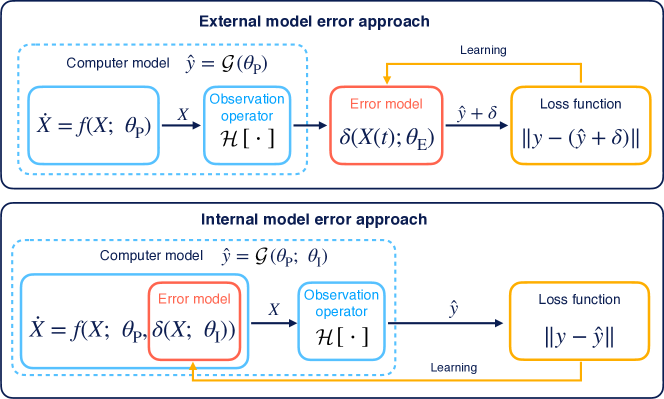
Such an approach has found applications, for example, in turbulence modeling [21, 22, 23, 24, 25, 26, 27]. By incorporating the structural error models $\delta(X;\ \theta_{\textrm{I}})$ inside the dynamical system, the error models can in principle lead to improved predictions even of quantities that were not used to train the error models. The error models can be learned alongside the model parameters $\theta_{\textrm{P}}$ in an online setting. They also are more amenable to interpretation because they are included in the places where errors are actually made. A potential downside of internalizing model error is that the effects of the structural errors $\delta$ map onto data $y$ only through the resolved state $X$ of the dynamical system, and residuals $y-\hat{y}$ are generally not directly informative about how the structural errors $\delta(X;\ \theta_{\textrm{I}})$ depend on state variables $X$; thus, learning about structural errors $\delta(X;\ \theta_{\textrm{I}})$ can generally not be accomplished with direct supervised learning approaches. Instead, residuals $y-\hat{y}$ only provide indirect information about structural errors $\delta(X;\ \theta_{\textrm{I}})$. Additionally, if derivatives of the dynamical system $f$ with respect to parameters are not easily available, or if the dynamical system is not differentiable, gradient-based methods for learning about the model errors $\delta(X;\ \theta_{\textrm{I}})$ are difficult or impossible to use.

Here we show various ways of constructing models for structural errors and demonstrate how one can learn about the structural errors from direct or indirect data in the absence of derivatives of the dynamical system. As error models, we will consider:

• Gaussian processes, as in Kennedy and O’Hagan [12];

• Models assembled from dictionaries of terms (e.g., involving differential operators), as in the data-driven discovery of partial differential equations [28, 29, 30, 31, 32, 33];

• Neural networks, for their expressivity [4, 34, 6, 7, 35, 36];

• Stochastic models, because without a clear scale separation between resolved and unresolved degrees of freedom, theoretical analysis suggests that closure models generally should be stochastic [e.g., 37, 38, 39, 40];

• Non-local models, because structural errors may be non-local in space [41, 42, 43, 44, 45], in time [46, 47, 48], or in both [49].

We will discuss how to learn about such error models both from direct and indirect data. Supervised learning of various types of error models $\delta_{l}$ from direct data has been performed in a number of settings, for example, to discover terms in differential equations or neural network closure models from residual time tendencies that give direct information about the error model that is sought [e.g., 50, 26, 27, 51]. However, data directly informative about error models, such as high-resolution time tendencies, are not always available. When training an error model on time tendencies, it can also be difficult to ensure both stability of the dynamical system including the error model and satisfaction of physical constraints (e.g., energy conservation) [e.g., 36]. Training an error model with indirect data, in an inverse problem rather than supervised learning setting [e.g., 24, 52, 53], can be advantageous in those circumstances. We demonstrate how it can be accomplished.

Our main contributions are:

• Summarizing the internal model error approach and comparing and contrasting it with the external model error approach.

• Presenting a comprehensive study of the internal model error approach for various model forms, including dictionary-based models, Gaussian processes, and neural networks, including non-local and stochastic generalizations.

• Demonstrating various methods for calibrating the internal model error, including (i) learning from direct data, (ii) learning from indirect data (e.g., moments of the time series for ergodic systems) with ensemble Kalman inversion (EKI), and (iii) learning from the time series of non-ergodic systems and using EKI for data assimilation (DA).

• Illustrating the importance of constraints (i.e., sparsity and known physics) for improved generalization of the calibrated internal model error.

The principles and algorithms we will discuss are broad purpose and applicable across a range of domains and model complexities. To illustrate their properties in a relatively simple setting, we use two versions of the Lorenz 96 [54] dynamical system: the basic version of the model and its multiscale generalization [55]. Section 2 discusses the calibration of internal error models with direct or indirect data and the enforcement of constraints such as conservation properties. Section 3 introduces various ways of constructing error models. Section 4 introduces two Lorenz 96 systems and then proceeds to present various concepts and methods through numerical results for these systems. The Lorenz 96 systems serve as illustrative examples of ergodic systems, for which we avoid trajectory matching and can demonstrate the use of time-averaged statistics, which approximate the expectation with respect to the invariant measure, as data from which to learn about the underlying unknown parameters. Section 5 is organized similarly to the previous section, but concerns non-ergodic systems for which trajectory matching is needed to learn about the underlying unknown parameters; in this context we study a model of the human glucose-insulin system. In Section 6, we state our conclusions.

2 Calibrating Error Models

We first summarize several important aspects of calibrating internal error models, including (i) direct or indirect data, (ii) gradient-based or derivative-free optimization, and (iii) enforcing constraints (e.g., sparsity or physical laws). We discuss these aspects with a generic internal error model $\delta(X;\theta_{\textrm{I}})$, which may represent any one of the error model types we will introduce later.

2.1 Data Availability

2.1.1 Direct Data

Direct data to calibrate $\delta$ are defined as “labeled” input-output pairs $\{X(t_{i}),\delta(X(t_{i}))\}_{i=1}^{N}$, where $i$ denotes a time index. Consider the additive error model

$$\dot{X}=f(X;\theta_{\textrm{P}})+\delta(X;\theta_{\textrm{I}})$$

as an example. A fine temporal resolution of $X(t)$ is usually needed to approximate $\dot{X}-f(X;\theta_{\textrm{P}})$ and obtain estimates of the error $\delta(X;\theta_{\textrm{I}})$ as a residual. With this method, it becomes challenging to obtain reliable direct data when the trajectories $\dot{X}$ are noisy, for example, when the dynamical system is chaotic [50]. Furthermore it may not be possible to observe the entirety of $X$. This may be handled as a missing data problem [56], and could be handled by joint parameter-state estimation for example using data assimilation; see [57, 58].

An additional complication with using direct data is ensuring the stability of the dynamical system with the calibrated error model $\delta(\cdot)$. Although with direct data, we can get more control of the accuracy of the error model itself, the calibrated error model often leads to unstable simulations of the dynamical system with the error model [59, 60]. There are several ways to mitigate the instability introduced by the error model, e.g., adopting a structure that ensures physical constraints [61], enforcing physical constraints [62], ensuring stability by bounding the eigenvalues of the linearized operator, and limiting the Lipschitz constant of $\delta(\cdot)$ [63]. However, a systematic approach to ensure stability is lacking.

2.1.2 Indirect Data

Instead of assuming access to direct data $\{X,\delta(X)\}$, the error model can also be calibrated with indirect data by solving an inverse problem associated with (6) (i.e., solve for the most likely parameters $\theta_{\textrm{P}},\theta_{\textrm{I}}$ given the model $\mathcal{G}$ and data $y$). Using indirect data involves simulating the dynamical system with the error model as in (5); therefore, the calibration procedure with indirect data favors error models that lead to stable simulations, an important advantage over the direct methods. Typical examples of problems giving rise to indirect data include time-series of $X$ for which the resolution is not fine enough to extract direct data for calibration [64], time-averaged statistics of $X$ [65] or dynamical systems that are partially observed [66]. More generally, indirect data can also be interpreted as constraints on $X$, and thus physical constraints can be enforced via augmenting indirect data.

2.2 Methods of Calibration

Using direct data $\{X,\delta(X)\}$ for calibration leads to a regression problem, which can be solved with standard methods for a given parameterization of the error model (e.g., least squares fit for dictionary learning, gradient descent methods for neural network). By contrast, using indirect data for calibration leads to an inverse problem associated with Eq. (6). Indirect methods can be linked to direct methods by framing the inverse problem as a missing data problem [56] and alternating between updating the missing data and updating the calibration parameters using learned direct data, for example, using the expectation-maximization (EM) algorithm [67]. However, in this section we focus on the calibration in the inverse problem setting; we discuss gradient-based and derivative-free optimization methods and how to enforce constraints.

2.2.1 Gradient-based or Derivative-free Optimization

Eq. (6) defines a forward problem in which $\mathcal{G},\theta_{\textrm{P}},\theta_{\textrm{I}}$ and noise $\eta$ can be used to generate simulated data. The associated inverse problem involves identifying the most likely parameters $\theta_{\textrm{P}},\theta_{\textrm{I}}$ for $\mathcal{G}$, conditioned on observed data $y$. To formalize this, we first define a loss function

$$\mathcal{L}(\theta)= \frac{1}{2}\bigl{|}y-\mathcal{G}\bigl{(}\theta_{\textrm{P}};\ \theta_{\textrm{I}}\bigr{)}\bigr{|}^{2}_{\Sigma},$$ (7)

where $\Sigma$ denotes the covariance of the zero-mean noise $\eta$, which is assumed to be independent of $\theta$. The inverse problem

$$\theta^{*}=\operatorname*{arg\,min}_{\theta}\mathcal{L}(\theta)$$

can be solved by gradient descent methods once the gradient

$$\frac{d\mathcal{L}}{d\theta}=\frac{d\mathcal{G}^{T}}{d\theta}\Sigma^{-1}(y-\mathcal{G})$$ (8)

is calculated, where $\theta=[\theta_{\textrm{I}},\theta_{\textrm{P}}]$ collects all parameters. In practice, the action of the gradient $d\mathcal{G}^{T}/d\theta$ is often evaluated via adjoint methods for efficiency. Although the gradient-based optimization is usually more efficient when $\mathcal{G}$ is differentiable, the evaluation of $\mathcal{G}$ can be noisy (e.g., when using finite-time averages to approximate infinite-time averaged data [68]) or stochastic (e.g., when using stochastic processes to construct the error model). In these settings, gradient-based optimization may no longer be suitable, and derivative-free optimization becomes necessary. In this paper we focus on Kalman-based derivative-free optimization for solving the inverse problem; A briefly reviews a specific easily implementable form of ensemble Kalman inversion (EKI), to illustrate how the methodology works, and gives pointers to the broader literature in the field.

2.2.2 Enforcing Constraints

There are various types of constraints that can be enforced when calibrating an error model. Two common constraints are sparsity constraints and physical constraints (e.g., conservation laws). Here we present the general concept of enforcing these two types of constraints in calibration, and A presents more details about using EKI to solve the corresponding constrained optimization problems.

Sparsity is important to impose on error models to avoid adding parameters to an error model that have no or little measurable impact on the output $\hat{y}$ of the host model; that is, the first principle in modeling structural errors should be to do no harm that would result from unnecessary error model complexity. To impose sparsity on the solution of $\theta_{\textrm{I}}$, we aim to solve the optimization problem [69]

$$\mathcal{L}(\theta;\lambda):= \frac{1}{2}\bigl{|}y-\mathcal{G}\bigl{(}\theta_{\textrm{P}};\ \theta_{\textrm{I}}\bigr{)}\bigr{|}^{2}_{\Sigma}+\lambda|\theta_{\textrm{I}}|_{\ell_{0}},$$ (9)

$$\theta^{*}= \operatorname*{arg\,min}_{\theta\in\mathfrak{V}}\mathcal{L}(\theta;\lambda),$$

where $\mathfrak{V}=\{\theta:|\theta_{\textrm{I}}|_{\ell_{1}}\leq\gamma\}$. The regularization parameters $\gamma$ and $\lambda$ can be determined via cross-validation. In practice, adding the $\ell_{0}$ constraint is achieved by thresholding the results from $\ell_{1}$-constrained optimization. The detailed algorithm was proposed in [69] and is summarized in A.

In many applications, it is important to find error models that satisfy physical constraints, such as energy conservation. To impose physical constraints on the solution of $\theta_{\textrm{I}}$ from EKI, we first generalize the constraint as:

$$\mathfrak{V}=\{\theta:\mathcal{R}(\theta_{\textrm{I}})\leq\gamma\}.$$ (10)

Here, $\mathcal{R}$ can be interpreted as a function that evaluates the residuals of certain physical constraints (typically, by solving Eq (5)). The constraint function $\mathcal{R}$ can be nonlinear with respect to $\theta_{\textrm{I}}$. Taking the additive error model $\dot{X}=f(X)+\delta(X;\theta_{\textrm{I}})$ as an example, the function $\mathcal{R}$ corresponding to the energy conservation constraint can be written explicitly as

$$\mathcal{R}(\theta_{\textrm{I}})=\Big{|}\int_{0}^{T}\big{(}\langle\delta(X(t);\theta_{\textrm{I}}),X(t)\rangle\big{)}dt\Big{|},$$ (11)

which constrains the total energy introduced into the system during the time interval $[0,T]$. Alternatively, a stronger constraint can be formulated as

$$\mathcal{R}(\theta_{\textrm{I}})=\int_{0}^{T}\big{|}\langle\delta(X(t);\theta_{\textrm{I}}),X(t)\rangle\big{|}dt,$$ (12)

which constrains the additional energy introduced into the system at every infinitesimal time step within the time interval $[0,T]$. The notation $\langle\cdot,\cdot\rangle$ denotes the inner product. Both forms of constraint in (11) and (12) can be implemented by using augmented observations, i.e., including the accumulated violation of the energy constraint as a additional piece of observation data whose true mean value is zero.

2.2.3 Accounting for Initial Conditions

Evaluation of $\mathcal{G}$ typically requires an initial condition, $X(0)$, when solving Eq. (5). When we observe ergodic systems over sufficiently long time scales, we can treat $\mathcal{G}$ as a stochastic map over a distribution of initial conditions [70]. However, when we observe systems over shorter time scales (or if they are non-ergodic), it is often necessary to identify initial conditions that generated the observations. We highlight two basic approaches: (i) append $X(0)$ to the vector of learned parameters for $\mathcal{G}$, and (ii) implicitly identify $X(0)$ by applying data assimilation techniques. To achieve (i), we can minimize:

$$\mathcal{L}\bigl{(}\theta,X(0)\bigr{)}=\frac{1}{2}\bigl{|}y-\mathcal{G}\bigl{(}\theta_{\textrm{P}};\ \theta_{\textrm{I}},X(0)\bigr{)}\bigr{|}^{2}_{\Sigma}.$$ (13)

To achieve (ii), we can minimize:

$$\mathcal{L}(\theta)= \frac{1}{2}\bigl{|}y-\mathcal{G}\bigl{(}\theta_{\textrm{P}};\ \theta_{\textrm{I}},X(0)\bigr{)}\bigr{|}^{2}_{\Sigma},$$ (14)

$$\textrm{s.t.}\ X(0)= \mathcal{DA}(\theta,y),$$

where $\mathcal{DA}$ represents a data assimilation algorithm that performs state estimation given observations $y$ and assumed parameters $\theta$. While Eqs. (13) and (14) appear quite similar, the utilization of efficient state-estimation algorithms in (14) can help cope with sensitivities to initial conditions that may cause (13) to fail. Recent work has explored different variants of (14), often using gradient-based optimization approaches and sequential state-estimation schemes [51, 71, 72, 58].

3 Constructing Error Models

We highlight three different approaches to representing structural errors: dictionary learning, Gaussian processes, and neural networks; however, other representations of structural error can also be considered within the overarching framework proposed here. For these three approaches, existing work mainly focuses on constructing deterministic error models that are locally dependent on state variables; however, the approaches can all be extended to the construction of stochastic error models or can be made non-locally dependent on state variables as described in Sections 3.4 and 3.5. For simplicity, we define the error models for the whole collection of structural errors $\delta(X,\theta_{\textrm{I}})$; however, we can also define and learn them independently for each component of the structural error model $\delta_{l}(X,\theta_{\textrm{I}}^{l})$ for $l=1,\dots,L$.

3.1 Dictionary Learning

If a set of candidate terms in error models is known or can be approximated, an error model can be constructed via learning from a dictionary of $J$ candidate terms,

$$\delta(X;\theta_{\textrm{I}})=\sum_{j=1}^{J}\alpha_{j}\phi_{j}(X;\beta_{j}),$$ (15)

where $\theta_{\textrm{I}}=\{\alpha,\beta\}$ and $\phi_{j}(X;\beta_{j})$ denote user-specified, parametric basis functions that can, for example, include differential operators [50, 29, 28, 30]. In practice, it is difficult to know all suitable basis functions a priori, and thus it is common to include redundant basis functions in the dictionary. Basis functions can then be pruned based on data by imposing sparsity constraints on the coefficients $\alpha_{j}$. Such sparsity constraints have proven to be beneficial in the construction of data-driven models of dynamical systems [50, 29, 28, 30, 69]. They are also commonly used in compressed sensing [73], where dictionary learning has been widely used.

An advantage of using dictionary learning is the potential interpretability of the constructed error model, arising because the error model is a linear combination of user-specified and hence interpretable basis functions. On the other hand, this approach can be overly restrictive when the dictionary of basis functions $\{\phi_{j}\}$ is misspecified, resulting in an insufficiently expressive error model.

3.2 Gaussian Processes

Another option of constructing an error model is via Gaussian processes (GPs) [74],

$$\delta(X;\theta_{\textrm{I}})\sim\mathcal{GP}\left(m,\mathcal{K}\right),$$ (16)

where $m:\mathcal{X}\mapsto\mathbb{R}$ denotes the mean of $\delta$, $\mathcal{K}:\mathcal{X}\times\mathcal{X}\mapsto\mathbb{R}$ represents a kernel, and $\mathcal{X}$ is the input space of the structural error model. Given data at $J$ different points $X^{(j)}$ for $j=1,2,...,J$, the mean of the error model can be written as a linear combination of basis functions,

$$m(X)=\sum_{j}\alpha_{j}\mathcal{K}(X^{(j)},X;\psi),$$ (17)

where $\psi$ denotes the hyper-parameters of the kernel $\mathcal{K}$. Therefore, the parameters that characterize the error model become $\theta_{\textrm{I}}=\{\alpha,\psi\}$ if the mean of a GP is used to represent the model error term $\delta$. The GP approach requires the choice of a kernel $\mathcal{K}$, which then determines the kernel functions $\mathcal{K}(X^{(j)},\cdot)$ in Eq. (17). This may appear restrictive, but the hyper-parameters of $\mathcal{K}$ are learned from the data; thus, the set of functions in which the solution is sought is data-adapted. This confers a potential advantage over dictionary learning, in particular for problems lacking in strong prior knowledge about the functional form of the model $\delta(X;\theta_{\textrm{I}})$ to be learned. In the case of indirect data, the locations $X^{(j)}$ must also be chosen a priori (or learnt as additional parameters).

Because of the similar forms of Eqs. (17) and (15), the GP shares similar shortcomings as dictionary learning when the kernel $\mathcal{K}$ is misspecified, even in the presence of hyper-parameter learning. In practice, a more sophisticated kernel $\mathcal{K}=\sum\limits_{i}\mathcal{K}_{i}$ is often constructed from some basic kernels $\mathcal{K}_{i}$ [75, 76, 77]. If a redundant set of basic kernels is used, sparsity constraints can be imposed in a similar way as in dictionary learning to prune the kernel set. A further limitation of using GPs is the computational cost, which grows exponentially with the dimension of $\mathcal{X}$. This pathology can be ameliorated by representing the GP as a linear combination of random Fourier features [78], which allows us to recast a GP as a dictionary-based approach in which the bases $\phi_{j}$ are drawn randomly from a special distribution known to reproduce a kernel of interest.

3.3 Neural Networks

Compared to dictionary learning, neural networks are more expressive, and they are more scalable than GPs, as the latter suffer from the curse of dimensionality if the model has high-dimensional input. Neural networks can also be used to construct an error model,

$$\delta(X;\theta_{\textrm{I}})=\mathcal{NN}(X;\theta_{\textrm{I}}),$$ (18)

where $\mathcal{NN}$ denotes a neural network and $\theta_{\textrm{I}}$ the coefficients (biases and weights) of the neural network. While neural networks are expressive and scalable, it is more difficult to enforce stability of a dynamical system with a neural network error model [60]. This is mainly because the nonlinearity introduced by a neural network is often more difficult to analyze compared with dictionary learning, for which we explicitly specify basis functions and thus can avoid using those that lead to instability; it is also more difficult to analyze than GP based learning because the latter is easier to interpret, as the kernels are hand-picked and then tuned to data. In Section 2.2.2, we discuss a general approach to enhancing stability by enforcing energy constraints in the context of learning from indirect data.

3.4 Stochastic Extension

In the preceding sections, we briefly summarized commonly used tools for constructing error models. All of those models were deterministic, with fixed parameters $\theta_{\textrm{I}}$. To quantify uncertainties, we can take a Bayesian perspective, view the unknown parameters as random variables, and infer the distributions of those parameters given the data. We can then propagate the uncertainties of those parameters to the simulated state $X$ and predicted observations $\hat{y}$ via Monte Carlo simulations. Although this is a standard approach to quantifying uncertainties, it cannot directly account for the impact of neglected information of unresolved scales upon the resolved state $X$. The randomness of the unresolved state can have an order one impact upon $X$; this issue is particularly prevalent in applications without a clear scale separation, such as turbulence, but can also happen in scale-separated problems. In such a scenario, directly modeling this impact as randomness in the resolved state becomes more appropriate, and it can be achieved by further adding a stochastic process to the deterministic error model:

$$\delta\Big{(}X;\theta_{\textrm{I}}\Big{)}\mathrm{d}t=\delta_{\mathrm{det}}(X;\theta_{\mathrm{det}})\mathrm{d}t+\sqrt{\sigma^{2}(X;\theta_{\mathrm{ran}})}\mathrm{d}W,$$ (19)

where $\mathrm{det}$ indicates a deterministic model, $W$ denotes the Wiener process, and the overall unknown parameters are defined as $\theta_{\textrm{I}}=\{\theta_{\mathrm{det}},\theta_{\mathrm{ran}}\}$. In practice, the above formulation can be further generalized by using stochastic processes (e.g., with desired temporal correlations) other than the Wiener process.

Fitting stochastic models to time-series data has been explored in some previous works [79, 80, 81, 82]; a common problem when applying these methods is the inconsistency between data and the incremental structure of the Gaussian noise driving the model as the time step is approaching zero [83, 84, 85, 86]. A common practice to address this issue is the multi-scale use of data, e.g., via subsampling [87, 66, 88, 89, 90, 91]. Some previous works also explored Kramers–Moyal averaging with finite sampling rate correction [92, 93, 94]. On the other hand, fitting a discretized version of stochastic processes to time-series data has been explored using autoregressive models [95, 96, 97, 98]. For some dynamical systems, the unresolved state has conditional (with respect to the resolved state) Gaussian statistics [99, 100], and then fitting the stochastic models can be achieved using analytically derived likelihoods.

In the absence of the whole trajectories of time series, some recent works started to explore fitting stochastic models to statistics of time-series data [101, 102, 103, 52]. Using time-averaged data to estimate linear SDEs has been studied for decades to account for climate variability [104, 105, 106, 107], and extension to nonlinear SDEs was discussed in [108].

3.5 Representing Non-local Effects

Spatial Non-locality

The states $X(t)$ for approximate models and their structural corrections typically consider $X(t)$ as a discretized spatial field. Most traditional closure models are formed locally; that is, they rely on the assumption of local dependence on $X(t,r)$, where $X(t,\cdot):\mathbb{R}^{p}\mapsto\mathbb{R}$ is a spatial field, and $r\in\mathbb{R}^{p}$ represents the spatial coordinate. For some applications, it is useful to consider non-local effect in the error model. Indeed, our formulations of the approximate physical model in (1) and models for structural error in Sections 3.1 to 3.3 are well-specified for scalar (local, component-wise) or vector-valued (non-local) $X$. Moreover, we note that non-local functions of the state $X(t)$ are best conceptualized as function-valued operators—while they take as inputs a vector of neighboring coordinates from $X(t)$, this vector represents a discretized spatial function. Thus, when designing spatially non-local closures, it is often sensible to build them to be consistent across different spatial discretizations.

In the case of neural networks, we can build spatially non-local closures with convolutional neural networks (CNNs); the Fourier neural operator (FNO) [109] or deep operator network (DeepONet) [110] provide an extension to an operator limit. Similarly, GPs and random feature methods (a dictionary-based formulation of GPs) can be designed with spatially non-local vectorized inputs from $X(t)$. Recent theoretical work has also allowed these basic methods to be taken to a continuous operator limit [111, 112].

As an emerging topic in the context of data-driven modeling, some recent works have explored non-local diffusion [43, 44, 113, 45] and spatially non-local modeling [41, 42, 49]. In this work, we capture the spatially non-local dependence on $X$ via a data-driven convolution kernel:

$$\delta\Big{(}X(t,r);\theta_{\textrm{I}}\Big{)}=\int_{r^{\prime}\in\Omega}\delta_{\textrm{loc}}(X(t,r^{\prime});\theta_{\textrm{loc}})\mathcal{C}(r-r^{\prime};\theta_{\textrm{non-loc}})\,dr^{\prime}$$ (20)

where $\Omega\subset\mathbb{R}^{p}$ represents a subset of $\mathbb{R}^{p}$ that contains $r$, and $\mathcal{C}:\mathbb{R}^{p}\mapsto\mathbb{R}$ denotes a convolution kernel with hyper-parameters $\theta_{\textrm{non-loc}}$. The overall parameterization is defined by $\theta_{\textrm{I}}=\{\theta_{\textrm{loc}},\theta_{\textrm{non-loc}}\}$, such that the unknown parameters in the local error model $\delta_{\textrm{loc}}$ and the convolutional kernel $\mathcal{C}$ can be jointly estimated.

Note that hyper-parameters can be made state-dependent, so that $\theta_{\textrm{non-loc}}(X(t,r);\kappa)$; in this case, the additional unknowns $\kappa$ can be learned, appending them to $\theta_{\textrm{I}}$. Similarly, learning a nonlinear integral kernel has been discussed in [114] and shown to be a continuous generalization of the transformer architecture [115].

The form of non-local closure in (20) draws inspiration from a series of works about non-local modeling [113], in which $\delta_{\textrm{loc}}$ corresponds to a local Laplace operator. Some mathematical foundations of non-local operators and calculus were summarized in [113], and the connection to fractional differential operators was illustrated in [116].

Temporal Non-locality

Non-locality in time (memory) is also important. Generically, any form of variable elimination or coarse-graining results in memory effects which require, at each current point in time, integration of the entire time-history from the initial condition up to the current time [37]. Such memory effects are undesirable as they lead to computational algorithms that scale poorly with respect to length of the time interval. Markovian models that encapsulate memory can be constructed, for example, by introducing a recurrent neural network [51], or by the use of delay embedding [117]; such Markovian models are more computationally expedient. Temporally non-local modeling has received significant recent attention [46, 47, 49, 48]. If diffusion/advection mechanisms are present in the resolved system, memory effects of any state variable would manifest themselves in the state variables as a spatial non-locality. For this reason non-local models with a flexible enough kernel could potentially be used to capture memory effects, without significantly increasing the computational costs.

4 Lorenz 96 Systems as Illustrative Examples

For our simulation studies of structural model error, we consider two variants of the celebrated Lorenz 96 model [54], described in what follows.

4.1 Lorenz Models

We consider a multiscale Lorenz 96 model, together with a single-scale companion model, to illustrate the principles and algorithms described in the subsequent sections. In each case, we use an untruncated version of the model as the true data-generating model and a truncated version as the model in which structural error models are to be learned.

4.1.1 Multiscale Lorenz 96 Model

The Lorenz 96 multi-scale system [54] describes the evolution of a simplified atmospheric flow, which is periodic along latitude circles (space). It does so through one set of slow variables, $x_{k}$ ($k=1,\dots,K$), coupled to a set of fast variables, $z_{j,k}$ ($j=1,\dots,J$), whose indices label space coordinates:

$$\dot{x}_{k} =-x_{k-1}(x_{k-2}-x_{k+1})-x_{k}+F-hc\bar{z}_{k},$$ (21)

$$\frac{1}{c}\dot{z}_{j,k} =-bz_{j+1,k}(z_{j+2,k}-z_{j-1,k})-z_{j,k}+\frac{h}{J}x_{k}.$$

Reflecting the periodicity along latitude circles, the variables are periodic in their indices, with

$$x_{k+K}=x_{k},\qquad z_{j,k+K}=z_{j,k},\qquad z_{j+J,k}=z_{j,k+1}.$$ (22)

The coupling term $hc\bar{z}_{k}$ describes the impact of the fast dynamics on the slow dynamics, with only the average

$$\bar{z}_{k}=\frac{1}{J}\sum_{j=1}^{J}z_{j,k}$$ (23)

of the fast variables affecting the slow variables. To generate data, we work with the parameter choices $K=36$, $J=10$, and $F=b=10$ [54, 65]. The choices of $h$ and $c$ are summarized in Subsection 4.2 for different cases.

To study how to model structural errors, we consider a coarse-grained system in which we only simulate approximate versions $X_{k}$ of the slow variables $x_{k}$, neglecting the fast variables. The approximate slow variables are governed by the system,

$$\dot{X_{k}} =-X_{k-1}(X_{k-2}-X_{k+1})-X_{k}+F+\delta(X_{k},X_{k}^{-};\theta_{\textrm{I}}),$$ (24)

$$X_{k+K} =X_{k},$$

for $X_{k}^{-}=(X_{k-d},\cdots,X_{k-1},X_{k+1},\cdots,X_{k+d}).$ Here, $\delta(\cdot)$ is the error model that accounts for the missing multiscale interactions. If there is no dependence on $X_{k}^{-}$, the model is local; otherwise, we allow for non-local dependency with a stencil of width $d$ on either side of $X_{k}$. If specified correctly, the model error ensures that the resolved variables $X_{k}$ of the coarse-grained system (24) approximate the variables $x_{k}$ of the full data generating system (21)–(23). We will use data generated with the full system (21)–(23) to learn about the error model $\delta(\cdot)$ in the coarse-grained system (24).

As data $y=\mathcal{H}[x(\cdot)]$ we consider

$$\mathcal{H}[x(\cdot)]=\mathbb{E}\mathcal{F}(x(\cdot)),$$

where $\mathbb{E}$ denotes expectation with respect to the stationary distribution of $x(t)$ and $\mathcal{F}:\mathcal{X}_{\textrm{traj}}\mapsto\mathbb{R}^{q}$ is a function on the space of solution trajectories (i.e., $\mathcal{X}_{\textrm{traj}}:0^{+}\mapsto\mathcal{X}$). In this work, we use moments of the vector $x$ and the averaged auto-correlation function as data and employ a finite-time average to approximate the expectation $\mathbb{E}$:

1. We will use $m^{\textrm{th}}-$moments of the vector $x$, i.e., $\mathcal{F}_{m}(x)=\Pi_{k\in M}x_{k}$:

   $$\mathcal{H}[x(\cdot)]\approx\frac{1}{T}\int_{0}^{T}\Pi_{k\in M}x_{k}(t)\mathrm{d}t,$$

   where $x_{k}$ denotes the $k^{\textrm{th}}$ element of vector $x$, and $M$ is a subset of size $m$ comprising indices (repetition allowed) from $\{1,\cdots,K\}$.

2. We will also use autocorrelation function $\mathcal{F}_{ac}(x(\cdot))=x(t+\tau)\otimes x(t)$:

   $$\mathcal{H}[x(\cdot)]\approx\frac{1}{T}\int_{0}^{T}x(t+\tau)\otimes x(t)\mathrm{d}t.$$

   In this work, we only consider the autocorrelation of the same element in the vector $x$, i.e., $x_{k}(t+\tau)x_{k}(t)$.

4.1.2 Single-scale Lorenz 96 Model

The single-scale Lorenz 96 system does not include the fast variables. We use it to illustrate the combined use of direct and indirect data and the advantage of enforcing conservation constraints in error models. The single-scale Lorenz 96 system describes the evolution of the $x_{k}$ variables alone,

$$\dot{x}_{k} =-x_{k-1}(x_{k-2}-x_{k+1})-x_{k}+F,$$ (25)

$$\quad x_{k+K} =x_{k},$$

and we use it to generate data in the setting where $K=36$ and $F=10$.

As the truncated system, we will only assume that we know the linearized part of the dynamics, resulting in an approximate model of the form

$$\dot{X_{k}} =-X_{k}+F+\delta(X_{k-2},X_{k-1},X_{k+1},X_{k+2};\theta_{\textrm{I}}),$$ (26)

$$X_{k+K} =X_{k}.$$

Here, $\delta$ is the error model that models the missing quadratic terms; we note that we postulate the need to learn a single universal function $\delta$ to account for model error in each component of the equation, reflecting an a priori assumption about the homogeneity of the structural error with respect to $k.$ Since the error model $\delta$ accounts for the unknown convection term and thus should not introduce additional energy, the state variable $X_{k}$ is excluded from the inputs of $\delta$ in the $k$-th equation. We will use data generated from the untruncated system (25) to learn about the error $\delta$ in the truncated system (26). As data $y=\mathcal{H}[x(t)]$, we employ the same types of data (i.e., moments and autocorrelation of the vector $x$) as described in Section 4.2.2.

4.2 Numerical Results for Lorenz Models

Before presenting detailed numerical results for Lorenz systems, we summarize several highlights of our numerical results.

1. For a multiscale system with clear scale separation, local deterministic error models using either direct or indirect data lead to satisfactory model fits. Detailed results are presented in Figs. 2 and 3.

2. For a multiscale system with less clear scale separation, local deterministic error models using direct data or indirect data do not lead to satisfactory model fits. Detailed results are presented in Figs. 4 and 5. However non-local or stochastic error models do lead to satisfactory fits. Detailed results are presented in Figs. 6 to 8.

3. For the single-scale Lorenz model, we show how an energy constraint can be incorporated into the EKI learning framework and leads to enhanced calibration of the error model. Detailed results are presented in Figs. 9 to 11.

4.2.1 Lorenz 96 Multi-scale Model

We first study the multi-scale Lorenz 96 system. The numerical examples for the multi-scale Lorenz 96 system are as follows:

1. For $c=10$ and $h=1$ in the multi-scale Lorenz 96 system, a dictionary-learning-based model is trained as local deterministic error model $\delta(X_{k})$ using direct data ($\{x_{k},hc\overline{z}_{k}\}$), and a fully-connected neural network is trained using indirect data (first and second moments of the slow variable $x_{k}$). For the indirect data in this example, we assume partial observations of the first eight slow variables and include cross-terms of second moments (i.e., $\mathbb{E}(x_{i}x_{j})$ for different $i$ and $j$). The results are presented in Figs. 2 and 3.

2. For $c=3$ and $h=10/3$ in the multi-scale Lorenz 96 system, the scale separation between fast and slow variables becomes smaller and thus leads to a more challenging case. In this case, a fully-connected neural network is trained as the local deterministic error model $\delta(X_{k})$ using either direct data ($\{x_{k},hc\overline{z}_{k}\}$) or indirect data (first to fourth moments of the slow variable $x_{k}$ and the autocorrelation of $x_{k}$). For the indirect data in this and the next examples, we enable the full observation of all 36 slow variables and preclude the use of all cross-terms of second to fourth moments. The results are presented in Figs. 4 and 5.

3. For $c=3$ and $h=10/3$ in the multi-scale Lorenz 96 system, we train a non-local deterministic error model $\delta(X)=\sum_{k^{\prime}}\delta(X_{k^{\prime}})\mathcal{C}(k-k^{\prime};\theta_{\textrm{non-loc}})$, a local stochastic error model with additive noise $\delta(X_{k})+\sqrt{\sigma^{2}}\dot{W_{k}}$, and a local stochastic error model with multiplicative noise $\delta(X_{k})+\sqrt{\sigma^{2}(X_{k})}\dot{W_{k}}$, using indirect data (first to fourth moments of the slow variable $x_{k}$ and the autocorrelation of $x_{k}$). The results are presented in Figs. 6 to 8.

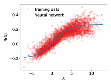
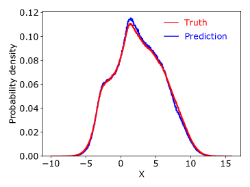
Figure 2a presents the direct data $\{x_{k},hc\bar{z}_{k}\}$. Based on direct data, a regression model $\delta(X_{k})$ can be trained and then used to simulate the dynamical system of $X_{k}$ in (24). In this work, we train such a regression model using a fully-connected neural network with two hidden layers (five neurons at the first hidden layer and one neuron at the second hidden layer). It can be seen in Fig. 2a that the trained model captures the general pattern of the training data. We also simulate the dynamical system in (24) for a long time trajectory and compare the invariant measure of $X_{k}$ with the true system in (21). As shown in Fig. 2b, we obtain a good agreement between the invariant measures of the modeled system and the true system.

(a) Trained model

(b) Invariant measure

Figure 2: Direct training of the error model ($c=10$) using a neural network, with results for (a) the trained error model and (b) the invariant measure.

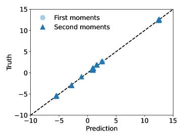
Because direct data $\{x_{k},hc\bar{z}_{k}\}$ may not be accessible in some applications, we also explore the use of indirect data to calibrate the error model $\delta(X_{k})$. In this example, the first and second moments of the first eight components of $x_{k}$ are used for the calibration. We tested different approaches that parameterize the error model $\delta(X_{k})$, including dictionary learning (Fig. 3), GPs and neural networks. The error model based on dictionary learning has the form $\delta(X_{k})=\sum_{i=1}^{2}\alpha_{i}\phi_{i}(X_{k})$, where we choose the basis function dictionary $\phi_{i}(X_{k})\in\{\tanh(\beta_{1}X_{k}),\tanh(\beta_{2}X_{k}^{2})\}$. Therefore, we have $\{\alpha_{i},\beta_{i}\}_{i=1}^{2}$ as unknown parameters to be learned. Instead of using polynomial basis functions, we have introduced the hyperbolic tangent function $\tanh(\cdot)$ to enhance the numerical stability. The error model based on a GP has the form $\delta(X_{k})=\sum_{j=1}^{7}\alpha_{j}\mathcal{K}(X_{k}^{(j)},X_{k};\ \psi)$, where we chose the $X_{k}^{(j)}$ as seven fixed points uniformly distributed in $[-15,15]$, and $\mathcal{K}$ as a squared exponential kernel with unknown constant hyper-parameters $\psi=\{\sigma_{\mathrm{GP}},\ell\}$, where $\sigma_{\mathrm{GP}}$ denotes the standard deviation and $\ell$ the length scale of the kernel. The results with a GP and with a neural network are similar to the ones with dictionary learning in Fig. 3 and are omitted here. The calibrated models in all three tests lead to good agreement in both data and invariant measure, and the performance of the calibrated model is not sensitive to the specific choice of parameterization approaches.

(a) Data comparison

(b) Invariant measure

Figure 3: Indirect training of the error model ($c=10$) using dictionary learning, with the results for (a) first and second moments and (b) the invariant measure. The results with a GP and a neural network have similar performance and are omitted.

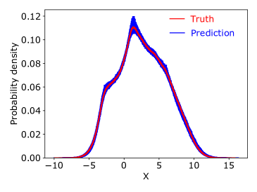
Although the performance of the calibrated error model is not sensitive to either the types of data or the parameterization approaches for this numerical example, the specific choices made in constructing and calibrating error models are still important, and even more so for more challenging scenarios, e.g., when the resolved and unresolved degrees of freedom have less scale separation.

To illustrate the advantage of using indirect data and stochastic/non-local error models, we study a more challenging scenario where the scale separation between $x_{k}$ and $y_{j,k}$ in (21) is narrower, by setting $h=10/3$ and $c=3$. It can be seen in Fig. 4a that the general pattern of the direct data is still captured by the trained error model $\delta(X_{k})$. However, the comparison of the invariant measures in Fig. 4b shows that the long-time behaviour of the trained model does not agree with the true system, indicating the limitation of using only direct data for the calibration.

(a) Trained model

(b) Invariant measure

Figure 4: Direct training of the error model ($c=3$) using a neural network, with results for (a) the trained error model and (b) the invariant measure.

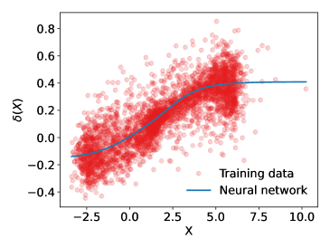
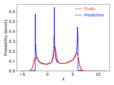
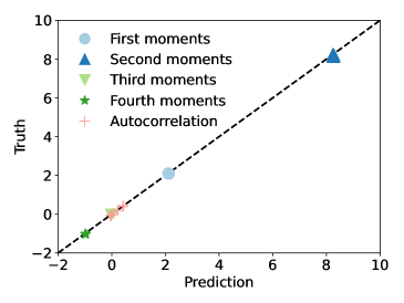
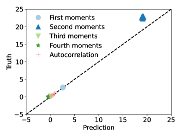
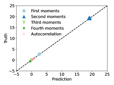
We further investigate the use of indirect data. Specifically, the first four moments of $X_{k}$ and ten points sampled from the averaged autocorrelation function of $X_{k}$ are used as training data. Figure 5 presents the results for the calibrated local model $\delta(X_{k})$. It can be seen in Fig. 5a that the trained error model agrees with the training data, while the invariant measures in Fig. 5b still differ between the calibrated and the true systems, indicating overfitting of the training data.

(a) Data comparison

(b) Invariant measure

Figure 5: Indirect training of the error model ($c=3$) using a deterministic model (local), with the results for (a) the first four moments and autocorrelation, and (b) the invariant measure.

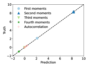
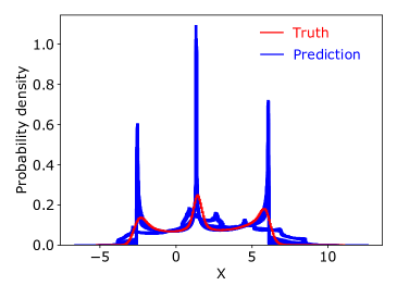
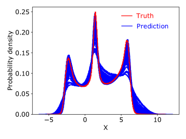
To avoid the overfitting in Fig. 5, we calibrate a non-local error model, as discussed in Section 3.5. Compared to the results for the local error model, it can be seen in Fig. 6 that the invariant measure of the calibrated system agrees better with the true system, which indicates that the closure model $\delta(\cdot)$ in (24) with non-local effects represents a better closure for unresolved scales if there is a less clear scale separation between resolved and unresolved scales.

(a) Data comparison

(b) Invariant measure

Figure 6: Indirect training of the error model ($c=3$) using a non-local deterministic model, with results for (a) the first four moments and autocorrelation, and (b) the invariant measure.

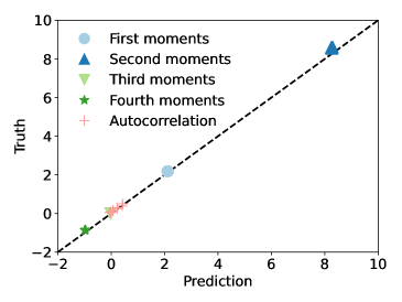
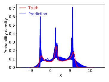
We also explored the learning of stochastic error model for this example. Figure 7 presents the results of the calibrated system with an additive stochastic error model. Compared to the results for deterministic error models in Figs. 5 and 6, we can see that the invariant measure of the calibrated system agrees better with the true system in Fig. 7b. We further test the stochastic error model by also learning a state-dependent diffusion coefficient. As shown in Fig. 8b, the calibrated system achieves better agreement with the invariant measure of the true system, which confirms that increased flexibility in the stochastic error model can help achieve improved predictive performance via training against indirect data. It should be noted that Figs. 6 to 8 do not display a single converged invariant measure. This arises because the calibrated parameters vary across the ensemble; as a result, we obtain a family of structural error models that all fit the data with similar accuracy. We surmise that this is caused by the fact that the indirect data contain only partial information about the invariant measure. Nonetheless, the fits are all far superior to those obtained with the local deterministic model.

(a) Data comparison

(b) Invariant measure

Figure 7: Indirect training of the error model ($c=3$) using stochastic model with additive noise, with the results for (a) the first four moments and autocorrelation, and (b) the invariant measure.

(a) Data comparison

(b) Invariant measure

Figure 8: Indirect training of the error model ($c=3$) using a stochastic model with multiplicative noise, with the results for (a) the first four moments and autocorrelation, and (b) the invariant measure.

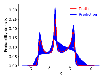
4.2.2 Lorenz 96 Single-scale Model

We studied the Lorenz 96 single-scale system to learn the quadratic term as an error model. Using this numerical example, we demonstrate the merit of combined use of direct and indirect data and the importance of enforcing physical constraints. More specifically, we assume that the quadratic term of the true system in (25) is unknown and then calibrate an error model $\delta(X_{k-2},X_{k-1},X_{k+1},X_{k+2})$ as in (26). The numerical examples for the single-scale Lorenz 96 system are as follows:

1. We train a fully-connected neural network as an error model $\delta(\cdot)$ using time-series of $x_{k}$ and the true quadratic term as direct data. The results are presented in Fig. 9.

2. We train a fully-connected neural network as an error model $\delta(\cdot)$ using indirect data (first to fourth moments of the state variable $x_{k}$ and the autocorrelation of $x_{k}$). The results are presented in Fig. 10.

3. We train a fully-connected neural network as an error model $\delta(\cdot)$ using indirect data (first to fourth moments of the state variable $x_{k}$ and the autocorrelation of $x_{k}$) and the energy conservation constraint in (12). The results are presented in Fig. 11.

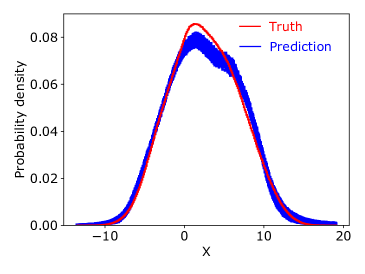
Figure 9 presents the comparison of invariant measures between the calibrated system and the true system when a fully connected neural network is used as an error model and is learned from direct data. As seen in Fig. 9, the calibrated system using direct data still differs noticeably in the invariant measure, indicating a difference from the long-time behavior of the true system.

Figure 9: Invariant measures via direct training of the error model ($c=10$) for the single-scale Lorenz 96 system.

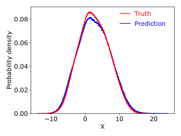
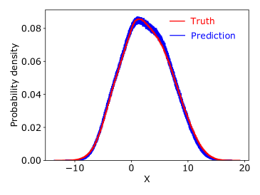
In order to improve the results of Fig. 9, we incorporate indirect data about the $x_{k}$. Specifically, we employ the trained model using direct data as the prior mean of EKI, and we set the prior standard deviation as $30\%$ of the mean values for each unknown coefficient of the error model. We then use EKI to calibrate the error model based on the first four moments of $X_{k}$ and the ten sampled points from the autocorrelation function of $X_{k}$. Without enforcing energy conservation of the error model, we can see in Fig. 10b that the performance of the calibrated model is similar to the calibrated system using direct data in Fig. 9. On the other hand, we also performed the calibration based on indirect data and enforced the energy conservation of the error model as discussed in Section 2.2.2. Considering that the true system conserves quadratic energy at every time, the energy constraint with the form in Eq. (12) is used. As shown in Fig. 11, the calibrated error model with energy conservation leads to a modeled system that better fits the training data and achieves a good agreement with the invariant measure of the true system.

(a) Data comparison

(b) Invariant measure

Figure 10: Results from trained error model ($c=10$) for the single-scale Lorenz 96 system without energy conservation constraint, including (a) first four moments and autocorrelation, and (b) invariant measures.

(a) Data comparison

(b) Invariant measure

Figure 11: Results from trained error model ($c=10$) for the single-scale Lorenz 96 system with energy conservation constraint, including (a) first four moments and autocorrelation, and (b) invariant measures.

5 Human Glucose-Insulin Model as Illustrative Example

The examples based on Lorenz systems in Section 4 illustrate the construction and calibration of internal error models for chaotic and ergodic systems, which are representative of a wide range of applications, e.g., in weather forecasting and climate change prediction, design of hypersonic vehicles, or the control of unmanned vehicles in a turbulent environment. However, there is another large class of applications for which the systems are non-ergodic and the goal is to accurately predict the time series of the system evolution. To achieve this goal for non-ergodic systems, we can no longer neglect the impact of the initial condition. We use a human glucose-insulin model as an example of a non-ergodic system and illustrate how the internal error model can be calibrated based on time series data, using EKI combined with data assimilation techniques.

5.1 Ultradian Model

We consider the ultradian model of the glucose-insulin system proposed in [118]. Its primary state variables are the plasma glucose concentration, $G$, the plasma insulin concentration, $I_{p}$, and the interstitial insulin concentration, $I_{i}$. These three state variables are augmented with a three stage delay $(h_{1},h_{2},h_{3})$ which encodes a non-linear delayed hepatic glucose response to plasma insulin levels. The resulting ordinary differential equations have the form:

$$\frac{dI_{p}}{dt} =f_{1}(G)-E\Big{(}\frac{I_{p}}{V_{p}}-\frac{I_{i}}{V_{i}}\Big{)}-\frac{I_{p}}{t_{p}}$$ (27a)

$$\frac{dI_{i}}{dt} =E\Big{(}\frac{I_{p}}{V_{p}}-\frac{I_{i}}{V_{i}}\Big{)}-\frac{I_{i}}{t_{i}}$$ (27b)

$$\frac{dG}{dt} =-f_{2}(G)-f_{3}(I_{i})G+f_{4}(h_{3})+m_{G}(t)$$ (27c)

$$\frac{dh_{1}}{dt} =\frac{1}{t_{d}}(I_{p}-h_{1})$$ (27d)

$$\frac{dh_{2}}{dt} =\frac{1}{t_{d}}(h_{1}-h_{2})$$ (27e)

$$\frac{dh_{3}}{dt} =\frac{1}{t_{d}}(h_{2}-h_{3})$$ (27f)

Here $m_{G}(t)$ represents a known rate of ingested carbohydrates appearing in the plasma, $f_{1}(G)$ represents the rate of glucose-dependent insulin production, $f_{2}(G)$ represents insulin-independent glucose utilization, $f_{3}(I_{i})G$ represents insulin-dependent glucose utilization, and $f_{4}(h_{3})$ represents delayed insulin-dependent hepatic glucose production. The functional forms of these parameterized processes are shown in B.

We represent a potential structural error in this model by removing the final linear term in (27a) (i.e., $t_{p}=\infty$). We then aim to identify a neural-network-based additive correction term for (27a), denoted by $\delta(I_{p},I_{i},G,h_{1},h_{2},h_{3};\theta)$. We calibrate $\delta(\cdot\ ;\ \theta)$ using partial, noisy observations of the physiologic state at times $\{t_{k}\}_{k=0}^{K}$. Specifically, we observe only the glucose state, $G(t)$, (it is the only state variable that is reliably measurable in patients) and add i.i.d. unit-Gaussian noise. Thus the observation operator $\mathcal{H}$ in Eq. (2) is defined through observation matrix $H\in\mathbb{R}^{1\times 6}$. To be specific $HX(t)=X_{3}(t)$ where $X(t)=[I_{p}(t),I_{i}(t),G(t),h_{1}(t),h_{2}(t),h_{3}(t)]^{T}$ and then $\mathcal{H}[X]=\{HX(t_{k})\}_{k=0}^{K}.$ It should be noted that the observation matrix $H$ projects between the full system state space and the observable space and may be used in the definition of a gain matrix $K$ for Kalman methods and generalizations such as 3DVAR (See Table 9.1 in [119]).

We refer to the observed data as $y=\big{[}y(t_{1}),\cdots,y(t_{K})\big{]}$ and to the solution of the entire six dimensional dynamical system at the observation times as $\big{[}x(t_{1}),\cdots,x(t_{K})\big{]}.$ We infer parameters $\theta$ by minimizing a variant of the loss defined in Eq. (14) in which the forward model itself depends on $y$:

$$\mathcal{L}(\theta)=\frac{1}{2}\bigl{|}y-\mathcal{G}\bigl{(}\theta;\ y\bigr{)}\bigr{|}^{2}_{\Sigma}.$$ (28)

Specifically $\mathcal{G}_{k}(\theta;\ y)$ uses sequential data assimilation to combine previous observations $\big{[}y(t_{1}),\cdots,y(t_{k-1})\big{]}$ with parameters $\theta$ to produce a filtered estimate for $x(t_{k-1})$ and, from this, predict the observation $y(t_{k})$; see section 2.2.3. The minimization of Eq. (28) is performed using EKI, where each evaluation of $\mathcal{G}(\theta;y)$ involves running a data assimilation sub-routine (3DVAR [119] with constant gain $K=[0,0,1,0,0,0]$).

5.2 Numerical Results for Ultradian Model

Through the presented numerical experiments in this section, we find that:

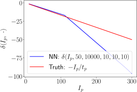
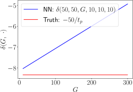
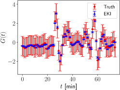
1. Model corrections can be learned for non-ergodic, non-stationary systems from noisy, partial observations of transient dynamics by applying DA as a sub-routine within the model inference pipeline (Figure 12).

2. Key structural components of model error terms can be identified despite being unobserved (Figure 12a).

3. Learned model error structure can exhibit inaccuracies outside of the observed data distribution and when models are insensitive to these inaccuracies (Figure 12b).

Figure 12 presents results from a trained model obtained by minimizing (28) via EKI. Figure 12c shows the transient trajectory data used to calibrate the model error, along with the obtained next-step predictions, which are seen to be highly accurate. Figure 12a shows that the neural network captures the true missing linear term $-I_{p}/t_{p}$ quite accurately in a wide range of inputs $I_{p}$, but is inaccurate where no data are available. Figure 12b shows the neural network as a function of an inactive input $G$ (an input upon which the true missing term does not depend); while it learns to correctly ignore $G$ in some of the plotted scenarios, it has spurious behavior outside of the observed range ($>200$) of $G$. Other results (not shown) indicate that the neural network learned substantial dependencies on inactive variables. This suggests that sparsity constraints may be useful in these experiments.

(a) Trained model: $\delta$ vs $I_{p}$

(b) Trained model: $\delta$ vs $G$

(c) Glucose trajectory fits: $G(t)$

Figure 12: Partial, noisy, transient timeseries data were used to calibrate model error. Results in (a-b) show the trained neural network error model for two specific input scenarios and (c) shows next-step predictions of $G$ from sequential data assimilation using the trained model. Figures (a-b) plot the model $\delta$ (a function of all 6 state variables) for 5 fixed states while varying $I_{p}$ and $G$, respectively.

6 Conclusions

Complex nonlinear dynamics and/or a large number of degrees of freedom are present in many systems, for example, in physiological models of the human body and turbulent flows around an airplane or in the wake of wind turbines. Typically, closure models are needed if some dynamically important degrees of freedom cannot be resolved by direct numerical simulations. Without a clear scale separation between resolved and unresolved degrees of freedom, most existing models, which are, semi-empirical, deterministic and local and are calibrated with only limited amounts of data, are not sophisticated enough to capture the true dynamics of the system. Incorporating models of structural errors that are informed by data can be an effective way to build on domain knowledge while using data more extensively.

We have summarized some key aspects of learning structural error models from data, including the construction of error models and their calibration. In doing so, we have provided guidelines about how to learn error models for complex dynamical systems, ranging from key insights about the incorporation of sparsity constraints (“do no harm”) and physical constraints, to advanced aspects such as the combined use of direct and indirect data and the merit of using non-local/stochastic error models. By addressing these varied aspects in a systematic manner, our goal has been to inspire further applied, methodological and theoretical research in this area.

Acknowledgments

TS, AMS, and JW were supported by the generosity of Eric and Wendy Schmidt by recommendation of the Schmidt Futures program. AMS is also supported by the Office of Naval Research (ONR) through grant N00014-17-1-2079 and by a Department of Defense Vannevar Bush Faculty Fellowship. MEL was supported by the National Science Foundation Graduate Research Fellowship under Grant No. DGE-1745301 and by funding from the Eric and Wendy Schmidt Center at the Broad Institute of MIT and Harvard.

All codes are available at:
https://github.com/jinlong83/Learning-Structural-Errors.git.

Appendix A Ensemble Kalman inversion

The use of ensemble Kalman based methods for parameter calibration and the solution of inverse problems, and history of this subject, is overviewed in [Section 4][120]. To be concrete we will concentrate on a particular variant of the methodology, sometimes termed Ensemble Kalman inversion (EKI). This is a specific ensemble-based, gradient-free optimization scheme that was proposed and studied in [121]; we emphasize that other ensemble Kalman based methods share the core desirable attributes of EKI, namely that it is derivative-free, is effective with relatively few evaluations of the forward model $\mathcal{G}$ and is robust to the presence of noise in the evaluations of $\mathcal{G}.$

The core task of EKI is equivalent to a quadratic optimization problem, which facilitates adding linear equality and inequality constraints [122]. To explain the details of EKI, we first introduce a new variable $w=\mathcal{G}(\theta)$ and variables $v$ and $g(v)$:

$$v =(\theta,w)^{\top},$$ (29)

$$g(v) =\left(\theta,\mathcal{G}(\theta)\right)^{\top}.$$

Using these variables we formulate the following noisily observed dynamical system:

$$v_{m+1} =g(v_{m})$$ (30)

$$y_{m+1} =Hv_{m+1}+\eta_{m+1}.$$

Here $H=[0,I],H^{\perp}=[I,0]$, and hence $Hv=w,H^{\perp}v=\theta.$ In this setting, $\{v_{m}\}$ is the state and $\{y_{m}\}$ are the data. The objective is to estimate $H^{\perp}v_{m}=\theta_{m}$ from $\{y_{\ell}\}_{\ell=1}^{m}$ and to do so iteratively with respect to $m$. In practice we only have one data point $y$ and not a sequence $y_{m}$; we address this issue in what follows below.

The EKI methodology creates an ensemble $\{v_{m}^{(j)}\}_{j=1}^{J}$ defined iteratively in $m$ as follows:

$$L_{m}^{(j)}(v):= \frac{1}{2}\big{|}y^{(j)}_{m+1}-Hv\big{|}^{2}_{\Gamma}+\frac{1}{2}\big{|}v-g\bigl{(}{v}_{m}^{(j)}\bigr{)}\big{|}^{2}_{C^{gg}_{m}},$$ (31)

$$v_{m+1}^{(j)}= \operatorname*{arg\,min}_{v}L_{m}^{(j)}(v).$$

The matrix $C^{gg}$ is the empirical covariance of $\{g(v_{m}^{(j)})\}_{j=1}^{J}$. The data $y^{(j)}_{m+1}$ is either fixed so that $y^{(j)}_{m+1}\equiv y$ or created by adding random draws to $y$ from the distribution of the $\eta$, independently for all $m$ and $j$. At each step, $m$ ensemble parameter estimates indexed by $j=1,\cdots,J$ are found from $\theta_{m}^{(j)}=H^{\perp}v_{m}^{(j)}.$

Using the fact that $v=(\theta,w)^{T}$, the minimizer $v_{m+1}^{(j)}$ in (31) decouples to give the update formula

$$\theta_{m+1}^{(j)}=\theta_{m}^{(j)}+C_{m}^{\theta\mathcal{G}}\left(C_{m}^{\mathcal{G}\mathcal{G}}+\Gamma\right)^{-1}\left(y_{m+1}^{(j)}-\mathcal{G}(\theta_{m}^{(j)})\right);$$ (32)

here the matrix $C_{m}^{\mathcal{G}\mathcal{G}}$ is the empirical covariance of $\{\mathcal{G}(\theta_{m}^{(j)})\}_{j=1}^{J}$, while matrix $C_{m}^{\theta\mathcal{G}}$ is the empirical cross-covariance of $\{\theta_{m}^{(j)}\}_{j=1}^{J}$ with $\{\mathcal{G}(\theta_{m}^{(j)})\}_{j=1}^{J}$.

To impose sparsity on the solution of $\theta$ from EKI, we solve the following constrained optimization problem after each EKI update step:

$$L_{m}^{(j)}(v,\lambda):= \frac{1}{2}\big{|}y^{(j)}_{m+1}-Hv\big{|}^{2}_{\Gamma}+\frac{1}{2}\big{|}v-g\bigl{(}{v}_{m}^{(j)}\bigr{)}\big{|}^{2}_{C^{gg}_{m}},$$ (33)

$$v_{m+1}^{(j)}= \operatorname*{arg\,min}_{v\in\mathfrak{V}}L_{m}^{(j)}(v),$$

where

$$\mathfrak{V}=\{v:|H^{\perp}v|_{\ell_{1}}\leq\gamma\}.$$ (34)

We also employ the thresholding function $\mathcal{T}$ on vectors defined by

$$\mathcal{T}(\theta_{i})=\begin{cases}0,&\text{if}\ |\theta_{i}|<\sqrt{2\lambda}\\ \theta_{i},&\text{otherwise},\end{cases}$$ (35)

to threshold those $\theta_{i}$ with values close to zero, after having solved the constrained optimization problem in (33). Such a thresholding step after the $\ell_{1}$-constrained optimization in (33) is equivalent to adding $\ell_{0}$ constraint. More details about imposing sparsity into EKI can be found in [69].

Appendix B Application to a Glucose-Insulin Model

The functional forms of the parameterized processes in Eq. (27) are as follows:

$$f_{1}(G) =\frac{R_{m}}{1+\exp\left(-\frac{G}{V_{g}c_{1}}+a_{1}\right)}$$ (rate of insulin production) (36)

$$f_{2}(G) =U_{1}\left(1-\exp\left(-\frac{G}{C_{2}V_{g}}\right)\right)$$ (insulin-independent glucose utilization) (37)

$$f_{3}(I_{i}) =\frac{1}{C_{3}V_{g}}\left(U_{0}+\frac{U_{m}-U_{0}}{1+(\kappa I_{i})^{-\beta}}\right)$$ (insulin-dependent glucose utilization) (38)

$$f_{4}(h_{3}) =\frac{R_{g}}{1+\exp\left(\alpha\left(\frac{h_{3}}{C_{5}V_{p}}-1\right)\right)}$$ delayed insulin-dependent glucose utilization (39)

$$\kappa =\frac{1}{C_{4}}\left(\frac{1}{V_{i}}-\frac{1}{Et_{i}}\right).$$ (40)

The uptake of carbohydates is modelled by the function

$$m_{G}(t)=\sum_{j=1}^{N(t)}\frac{m_{j}k}{60\ \text{min}}\exp(k(t_{j}-t)),\ \ N(t)=\#\{t_{j}<t\}$$ (41)

in which $N$ meals occur at times $\{t_{j}\}_{j=1}^{N}$ (in minutes), with carbohydrate composition $\{m_{j}\}_{j=1}^{N}$ (note that these typically differ from observation times).

References

- Schneider et al. [2017] T. Schneider, J. Teixeira, C. S. Bretherton, F. Brient, K. G. Pressel, C. Schär, A. P. Siebesma, Climate goals and computing the future of clouds, Nature Climate Change 7 (2017) 3–5.
- Smagorinsky [1963] J. Smagorinsky, General circulation experiments with the primitive equations. I. The basic experiment, Mon. Wea. Rev. 91 (1963) 99–164.
- Holtslag and Moeng [1991] A. Holtslag, C.-H. Moeng, Eddy diffusivity and countergradient transport in the convective atmospheric boundary layer, Journal of the Atmospheric Sciences 48 (1991) 1690–1698.
- Ling et al. [2016] J. Ling, A. Kurzawski, J. Templeton, Reynolds averaged turbulence modelling using deep neural networks with embedded invariance, Journal of Fluid Mechanics 807 (2016) 155–166.
- Weatheritt and Sandberg [2016] J. Weatheritt, R. Sandberg, A novel evolutionary algorithm applied to algebraic modifications of the RANS stress–strain relationship, Journal of Computational Physics 325 (2016) 22–37.
- Rasp et al. [2018] S. Rasp, M. S. Pritchard, P. Gentine, Deep learning to represent subgrid processes in climate models, Proc. Natl. Acad. Sci. (2018).
- Maulik et al. [2019] R. Maulik, O. San, A. Rasheed, P. Vedula, Subgrid modelling for two-dimensional turbulence using neural networks, Journal of Fluid Mechanics 858 (2019) 122–144.
- Duraisamy et al. [2019] K. Duraisamy, G. Iaccarino, H. Xiao, Turbulence modeling in the age of data, Annual Review of Fluid Mechanics 51 (2019) 357–377.
- Zhao et al. [2020] Y. Zhao, H. D. Akolekar, J. Weatheritt, V. Michelassi, R. D. Sandberg, RANS turbulence model development using CFD-driven machine learning, Journal of Computational Physics 411 (2020) 109413.
- Schmelzer et al. [2020] M. Schmelzer, R. P. Dwight, P. Cinnella, Discovery of algebraic Reynolds-stress models using sparse symbolic regression, Flow, Turbulence and Combustion 104 (2020) 579–603.
- Brunton et al. [2020] S. L. Brunton, B. R. Noack, P. Koumoutsakos, Machine learning for fluid mechanics, Ann. Rev. Fluid Mech. 52 (2020) 477–508.
- Kennedy and O’Hagan [2001] M. C. Kennedy, A. O’Hagan, Bayesian calibration of computer models, Journal of the Royal Statistical Society: Series B (Statistical Methodology) 63 (2001) 425–464.
- Higdon et al. [2004] D. Higdon, M. Kennedy, J. C. Cavendish, J. A. Cafeo, R. D. Ryne, Combining field data and computer simulations for calibration and prediction, SIAM Journal on Scientific Computing 26 (2004) 448–466.
- Wang et al. [2009] S. Wang, W. Chen, K.-L. Tsui, Bayesian validation of computer models, Technometrics 51 (2009) 439–451.
- Brynjarsdòttir and O’Hagan [2014] J. Brynjarsdòttir, A. O’Hagan, Learning about physical parameters: The importance of model discrepancy, Inverse problems 30 (2014) 114007.
- Trehan et al. [2017] S. Trehan, K. T. Carlberg, L. J. Durlofsky, Error modeling for surrogates of dynamical systems using machine learning, International Journal for Numerical Methods in Engineering 112 (2017) 1801–1827.
- Calvetti et al. [2018] D. Calvetti, M. Dunlop, E. Somersalo, A. Stuart, Iterative updating of model error for Bayesian inversion, Inverse Problems 34 (2018) 025008.
- Strong and Oakley [2014] M. Strong, J. E. Oakley, When is a model good enough? Deriving the expected value of model improvement via specifying internal model discrepancies, SIAM/ASA Journal on Uncertainty Quantification 2 (2014) 106–125.
- He and Xiu [2016] Y. He, D. Xiu, Numerical strategy for model correction using physical constraints, Journal of Computational Physics 313 (2016) 617–634.
- Sargsyan et al. [2019] K. Sargsyan, X. Huan, H. N. Najm, Embedded model error representation for Bayesian model calibration, International Journal for Uncertainty Quantification 9 (2019).
- Emory et al. [2011] M. Emory, R. Pecnik, G. Iaccarino, Modeling structural uncertainties in Reynolds-averaged computations of shock/boundary layer interactions, in: 49th AIAA Aerospace sciences meeting including the new horizons forum and aerospace exposition, 2011, p. 479.
- Oliver and Moser [2011] T. A. Oliver, R. D. Moser, Bayesian uncertainty quantification applied to RANS turbulence models, in: Journal of Physics: Conference Series, volume 318, IOP Publishing, 2011, p. 042032.
- Cheung et al. [2011] S. H. Cheung, T. A. Oliver, E. E. Prudencio, S. Prudhomme, R. D. Moser, Bayesian uncertainty analysis with applications to turbulence modeling, Reliability Engineering & System Safety 96 (2011) 1137–1149.
- Xiao et al. [2016] H. Xiao, J.-L. Wu, J.-X. Wang, R. Sun, C. Roy, Quantifying and reducing model-form uncertainties in Reynolds-averaged Navier–Stokes simulations: A data-driven, physics-informed Bayesian approach, Journal of Computational Physics 324 (2016) 115–136.
- Pernot and Cailliez [2017] P. Pernot, F. Cailliez, A critical review of statistical calibration/prediction models handling data inconsistency and model inadequacy, AIChE Journal 63 (2017) 4642–4665.
- Wang et al. [2017] J.-X. Wang, J.-L. Wu, H. Xiao, Physics-informed machine learning approach for reconstructing Reynolds stress modeling discrepancies based on DNS data, Physical Review Fluids 2 (2017) 034603.
- Wu et al. [2018] J.-L. Wu, H. Xiao, E. Paterson, Physics-informed machine learning approach for augmenting turbulence models: A comprehensive framework, Physical Review Fluids 3 (2018) 074602.
- Schaeffer et al. [2013] H. Schaeffer, R. Caflisch, C. D. Hauck, S. Osher, Sparse dynamics for partial differential equations, Proceedings of the National Academy of Sciences 110 (2013) 6634–6639.
- Rudy et al. [2017] S. H. Rudy, S. L. Brunton, J. L. Proctor, J. N. Kutz, Data-driven discovery of partial differential equations, Science Advances 3 (2017) e1602614.
- Schaeffer [2017] H. Schaeffer, Learning partial differential equations via data discovery and sparse optimization, Proceedings of the Royal Society A: Mathematical, Physical and Engineering Sciences 473 (2017) 20160446.
- Zanna and Bolton [2020] L. Zanna, T. Bolton, Data-driven equation discovery of ocean mesoscale closures, Geophysical Research Letters 47 (2020) e2020GL088376.
- de Silva et al. [2020] B. M. de Silva, D. M. Higdon, S. L. Brunton, J. N. Kutz, Discovery of physics from data: Universal laws and discrepancies, Front. Artif. Intell. 3 (2020) 25.
- Lemos et al. [2022] P. Lemos, N. Jeffrey, M. Cranmer, S. Ho, P. Battaglia, Rediscovering orbital mechanics with machine learning (2022).
- Brenowitz and Bretherton [2018] N. D. Brenowitz, C. S. Bretherton, Prognostic validation of a neural network unified physics parameterization, Geophysical Research Letters 45 (2018) 6289–6298.
- Zanna and Bolton [2021] L. Zanna, T. Bolton, Deep learning of unresolved turbulent ocean processes in climate models, Deep Learning for the Earth Sciences: A Comprehensive Approach to Remote Sensing, Climate Science, and Geosciences (2021) 298–306.
- Bretherton et al. [2022] C. S. Bretherton, B. Henn, A. Kwa, N. D. Brenowitz, O. Watt-Meyer, J. McGibbon, W. A. Perkins, S. K. Clark, L. Harris, Correcting coarse-grid weather and climate models by machine learning from global storm-resolving simulations, J. Adv. Model. Earth Sys. 14 (2022) e2021MS002794.
- Zwanzig [2001] R. Zwanzig, Nonequilibrium statistical mechanics, Oxford university press, 2001.
- Lucarini et al. [2014] V. Lucarini, R. Blender, C. Herbert, F. Ragone, S. Pascale, J. Wouters, Mathematical and physical ideas for climate science, Rev. Geophys. 52 (2014) 809–859.
- Franzke et al. [2015] C. L. Franzke, T. J. O’Kane, J. Berner, P. D. Williams, V. Lucarini, Stochastic climate theory and modeling, Wiley Interdisciplinary Reviews: Climate Change 6 (2015) 63–78.
- Palmer [2019] T. Palmer, Stochastic weather and climate models, Nature Reviews Physics 1 (2019) 463–471.
- Zhou et al. [2021] X.-H. Zhou, J. Han, H. Xiao, Learning nonlocal constitutive models with neural networks, Computer Methods in Applied Mechanics and Engineering 384 (2021) 113927.
- Zhuang et al. [2021] J. Zhuang, D. Kochkov, Y. Bar-Sinai, M. P. Brenner, S. Hoyer, Learned discretizations for passive scalar advection in a two-dimensional turbulent flow, Phys. Rev. Fluids 6 (2021) 064605.
- Du et al. [2012] Q. Du, M. Gunzburger, R. B. Lehoucq, K. Zhou, Analysis and approximation of nonlocal diffusion problems with volume constraints, SIAM Review 54 (2012) 667–696.
- D’Elia and Gunzburger [2016] M. D’Elia, M. Gunzburger, Identification of the diffusion parameter in nonlocal steady diffusion problems, Applied Mathematics & Optimization 73 (2016) 227–249.
- Pang et al. [2020] G. Pang, M. D’Elia, M. Parks, G. E. Karniadakis, nPINNs: nonlocal physics-informed neural networks for a parametrized nonlocal universal Laplacian operator. algorithms and applications, Journal of Computational Physics 422 (2020) 109760.
- Ma et al. [2018] C. Ma, J. Wang, et al., Model reduction with memory and the machine learning of dynamical systems, arXiv preprint arXiv:1808.04258 (2018).
- Wang et al. [2020] Q. Wang, N. Ripamonti, J. S. Hesthaven, Recurrent neural network closure of parametric POD-Galerkin reduced-order models based on the Mori-Zwanzig formalism, Journal of Computational Physics 410 (2020) 109402.
- Lin and Lu [2021] K. K. Lin, F. Lu, Data-driven model reduction, Wiener projections, and the Koopman-Mori-Zwanzig formalism, Journal of Computational Physics 424 (2021) 109864.
- Charalampopoulos and Sapsis [2021] A.-T. G. Charalampopoulos, T. P. Sapsis, Machine-learning energy-preserving nonlocal closures for turbulent fluid flows and inertial tracers, arXiv preprint arXiv:2102.07639 (2021).
- Brunton et al. [2016] S. L. Brunton, J. L. Proctor, J. N. Kutz, Discovering governing equations from data by sparse identification of nonlinear dynamical systems, Proceedings of the National Academy of Sciences 113 (2016) 3932–3937.
- Levine and Stuart [2022] M. Levine, A. Stuart, A framework for machine learning of model error in dynamical systems, Communications of the American Mathematical Society 2 (2022) 283–344.
- Schneider et al. [2021] T. Schneider, A. M. Stuart, J.-L. Wu, Learning stochastic closures using ensemble kalman inversion, Transactions of Mathematics and Its Applications 5 (2021) tnab003.
- Zhang et al. [2022] X.-L. Zhang, H. Xiao, X. Luo, G. He, Ensemble kalman method for learning turbulence models from indirect observation data, Journal of Fluid Mechanics 949 (2022) A26.
- Lorenz [1996] E. N. Lorenz, Predictability: A problem partly solved, in: Proc. Seminar on predictability, volume 1, 1996.
- Fatkullin and Vanden-Eijnden [2004] I. Fatkullin, E. Vanden-Eijnden, A computational strategy for multiscale systems with applications to lorenz 96 model, Journal of Computational Physics 200 (2004) 605–638.
- Little and Rubin [2019] R. J. Little, D. B. Rubin, Statistical analysis with missing data, volume 793, John Wiley & Sons, 2019.
- Bocquet et al. [2019] M. Bocquet, J. Brajard, A. Carrassi, L. Bertino, Data assimilation as a learning tool to infer ordinary differential equation representations of dynamical models, Nonlinear Processes in Geophysics 26 (2019) 143–162.
- Chen et al. [2022] Y. Chen, D. Sanz-Alonso, R. Willett, Autodifferentiable ensemble Kalman filters, SIAM Journal on Mathematics of Data Science 4 (2022) 801–833.
- Beck et al. [2019] A. Beck, D. Flad, C.-D. Munz, Deep neural networks for data-driven LES closure models, Journal of Computational Physics 398 (2019) 108910.
- Brenowitz et al. [2020] N. D. Brenowitz, T. Beucler, M. Pritchard, C. S. Bretherton, Interpreting and stabilizing machine-learning parametrizations of convection, Journal of the Atmospheric Sciences 77 (2020) 4357–4375.
- Yuval et al. [2021] J. Yuval, P. A. O’Gorman, C. N. Hill, Use of neural networks for stable, accurate and physically consistent parameterization of subgrid atmospheric processes with good performance at reduced precision, Geophysical Research Letters 48 (2021) e2020GL091363.
- Beucler et al. [2021] T. Beucler, M. Pritchard, S. Rasp, J. Ott, P. Baldi, P. Gentine, Enforcing analytic constraints in neural networks emulating physical systems, Physical Review Letters 126 (2021) 098302.
- Shi et al. [2019] G. Shi, X. Shi, M. O’Connell, R. Yu, K. Azizzadenesheli, A. Anandkumar, Y. Yue, S.-J. Chung, Neural lander: Stable drone landing control using learned dynamics, in: 2019 International Conference on Robotics and Automation (ICRA), IEEE, 2019, pp. 9784–9790.
- Boys et al. [2008] R. J. Boys, D. J. Wilkinson, T. B. Kirkwood, Bayesian inference for a discretely observed stochastic kinetic model, Statistics and Computing 18 (2008) 125–135.
- Schneider et al. [2017] T. Schneider, S. Lan, A. Stuart, J. Teixeira, Earth system modeling 2.0: A blueprint for models that learn from observations and targeted high-resolution simulations, Geophysical Research Letters 44 (2017) 12–396.
- Pokern et al. [2009] Y. Pokern, A. M. Stuart, P. Wiberg, Parameter estimation for partially observed hypoelliptic diffusions, Journal of the Royal Statistical Society: Series B (Statistical Methodology) 71 (2009) 49–73.
- Meng and Van Dyk [1997] X.-L. Meng, D. Van Dyk, The EM algorithm—an old folk-song sung to a fast new tune, Journal of the Royal Statistical Society: Series B (Statistical Methodology) 59 (1997) 511–567.
- Dunbar et al. [2022] O. R. Dunbar, A. B. Duncan, A. M. Stuart, M.-T. Wolfram, Ensemble inference methods for models with noisy and expensive likelihoods, SIAM Journal on Applied Dynamical Systems 21 (2022) 1539–1572.
- Schneider et al. [2022] T. Schneider, A. M. Stuart, J.-L. Wu, Ensemble Kalman inversion for sparse learning of dynamical systems from time-averaged data, Journal of Computational Physics 470 (2022) 111559.
- Cleary et al. [2021] E. Cleary, A. Garbuno-Inigo, S. Lan, T. Schneider, A. M. Stuart, Calibrate, emulate, sample, Journal of Computational Physics 424 (2021) 109716.
- Ribera et al. [2022] H. Ribera, S. Shirman, A. Nguyen, N. Mangan, Model selection of chaotic systems from data with hidden variables using sparse data assimilation, Chaos: An Interdisciplinary Journal of Nonlinear Science 32 (2022).
- Brajard et al. [2021] J. Brajard, A. Carrassi, M. Bocquet, L. Bertino, Combining data assimilation and machine learning to infer unresolved scale parametrization, Philosophical Transactions of the Royal Society A 379 (2021) 20200086.
- Donoho [2006] D. L. Donoho, Compressed sensing, IEEE Transactions on information theory 52 (2006) 1289–1306.
- Williams and Rasmussen [2006] C. K. Williams, C. E. Rasmussen, Gaussian processes for machine learning, volume 2, MIT press Cambridge, MA, 2006.
- Hamzi and Owhadi [2021] B. Hamzi, H. Owhadi, Learning dynamical systems from data: a simple cross-validation perspective, part i: parametric kernel flows, Physica D: Nonlinear Phenomena 421 (2021) 132817.
- Darcy et al. [2021] M. Darcy, B. Hamzi, J. Susiluoto, A. Braverman, H. Owhadi, Learning dynamical systems from data: a simple cross-validation perspective, part ii: nonparametric kernel flows, preprint (2021).
- Lee et al. [2022] J. Lee, E. De Brouwer, B. Hamzi, H. Owhadi, Learning dynamical systems from data: A simple cross-validation perspective, part iii: Irregularly-sampled time series, Physica D: Nonlinear Phenomena (2022) 133546.
- Rahimi and Recht [2008] A. Rahimi, B. Recht, Random Features for Large-Scale Kernel Machines, in: J. Platt, D. Koller, Y. Singer, S. Roweis (Eds.), Advances in Neural Information Processing Systems, volume 20, Curran Associates, Inc., 2008.
- Wilkinson [2009] D. J. Wilkinson, Stochastic modelling for quantitative description of heterogeneous biological systems, Nature Reviews Genetics 10 (2009) 122–133.
- Roberts and Stramer [2001] G. O. Roberts, O. Stramer, On inference for partially observed nonlinear diffusion models using the Metropolis–Hastings algorithm, Biometrika 88 (2001) 603–621.
- Roberts and Stramer [2002] G. O. Roberts, O. Stramer, Langevin diffusions and Metropolis-Hastings algorithms, Methodology and computing in applied probability 4 (2002) 337–357.
- Papaspiliopoulos et al. [2013] O. Papaspiliopoulos, G. O. Roberts, O. Stramer, Data augmentation for diffusions, Journal of Computational and Graphical Statistics 22 (2013) 665–688.
- Zhang et al. [2005] L. Zhang, P. A. Mykland, Y. Aït-Sahalia, A tale of two time scales: Determining integrated volatility with noisy high-frequency data, Journal of the American Statistical Association 100 (2005) 1394–1411.
- Pavliotis and Stuart [2007] G. A. Pavliotis, A. Stuart, Parameter estimation for multiscale diffusions, Journal of Statistical Physics 127 (2007) 741–781.
- Papavasiliou et al. [2009] A. Papavasiliou, G. Pavliotis, A. Stuart, Maximum likelihood drift estimation for multiscale diffusions, Stochastic Processes and their Applications 119 (2009) 3173–3210.
- Boninsegna et al. [2018] L. Boninsegna, F. Nüske, C. Clementi, Sparse learning of stochastic dynamical equations, The Journal of chemical physics 148 (2018) 241723.
- Zhang [2006] L. Zhang, Efficient estimation of stochastic volatility using noisy observations: A multi-scale approach, Bernoulli 12 (2006) 1019–1043.
- Papaspiliopoulos et al. [2012] O. Papaspiliopoulos, Y. Pokern, G. O. Roberts, A. M. Stuart, Nonparametric estimation of diffusions: a differential equations approach, Biometrika 99 (2012) 511–531.
- Pavliotis et al. [2012] G. A. Pavliotis, Y. Pokern, A. M. Stuart, Parameter estimation for multiscale diffusions: An overview, Statistical Methods for Stochastic Differential Equations (2012) 429.
- Batz et al. [2018] P. Batz, A. Ruttor, M. Opper, Approximate Bayes learning of stochastic differential equations, Physical Review E 98 (2018) 022109.
- Abdulle et al. [2021] A. Abdulle, G. Garegnani, G. A. Pavliotis, A. M. Stuart, A. Zanoni, Drift estimation of multiscale diffusions based on filtered data, Foundations of Computational Mathematics (2021) 1–52.
- Honisch and Friedrich [2011] C. Honisch, R. Friedrich, Estimation of Kramers-Moyal coefficients at low sampling rates, Physical Review E 83 (2011) 066701.
- Lade [2009] S. J. Lade, Finite sampling interval effects in Kramers–Moyal analysis, Physics Letters A 373 (2009) 3705–3709.
- Callaham et al. [2021] J. L. Callaham, J.-C. Loiseau, G. Rigas, S. L. Brunton, Nonlinear stochastic modelling with Langevin regression, Proceedings of the Royal Society A 477 (2021) 20210092.
- Neumaier and Schneider [2001] A. Neumaier, T. Schneider, Estimation of parameters and eigenmodes of multivariate autoregressive models, ACM Trans. Math. Softw. 27 (2001) 27–57.
- Schneider and Neumaier [2001] T. Schneider, A. Neumaier, Algorithm 808: ARfit — A Matlab package for the estimation of parameters and eigenmodes of multivariate autoregressive models, ACM Trans. Math. Softw. 27 (2001) 58–65.
- Arnold et al. [2013] H. Arnold, I. Moroz, T. Palmer, Stochastic parametrizations and model uncertainty in the Lorenz’96 system, Philosophical Transactions of the Royal Society A: Mathematical, Physical and Engineering Sciences 371 (2013) 20110479.
- Lu [2020] F. Lu, Data-driven model reduction for stochastic Burgers equations, Entropy 22 (2020) 1360.
- Chen and Majda [2016] N. Chen, A. J. Majda, Filtering nonlinear turbulent dynamical systems through conditional Gaussian statistics, Monthly Weather Review 144 (2016) 4885–4917.
- Chen and Majda [2018] N. Chen, A. J. Majda, Conditional Gaussian systems for multiscale nonlinear stochastic systems: Prediction, state estimation and uncertainty quantification, Entropy 20 (2018) 509.
- Krumscheid et al. [2013] S. Krumscheid, G. A. Pavliotis, S. Kalliadasis, Semiparametric drift and diffusion estimation for multiscale diffusions, Multiscale Modeling & Simulation 11 (2013) 442–473.
- Krumscheid et al. [2015] S. Krumscheid, M. Pradas, G. Pavliotis, S. Kalliadasis, Data-driven coarse graining in action: Modeling and prediction of complex systems, Physical Review E 92 (2015) 042139.
- Kalliadasis et al. [2015] S. Kalliadasis, S. Krumscheid, G. A. Pavliotis, A new framework for extracting coarse-grained models from time series with multiscale structure, Journal of Computational Physics 296 (2015) 314–328.
- Hasselmann [1976] K. Hasselmann, Stochastic climate models part i. theory, tellus 28 (1976) 473–485.
- Frankignoul and Hasselmann [1977] C. Frankignoul, K. Hasselmann, Stochastic climate models, part ii application to sea-surface temperature anomalies and thermocline variability, Tellus 29 (1977) 289–305.
- Penland and Magorian [1993] C. Penland, T. Magorian, Prediction of Niño 3 sea surface temperatures using linear inverse modeling, Journal of Climate 6 (1993) 1067–1076.
- Schneider and Griffies [1999] T. Schneider, S. M. Griffies, A conceptual framework for predictability studies, J. Climate 12 (1999) 3133–3155.
- Hasselmann [1988] K. Hasselmann, PIPs and POPs: The reduction of complex dynamical systems using principal interaction and oscillation patterns, Journal of Geophysical Research: Atmospheres 93 (1988) 11015–11021.
- Li et al. [2020] Z. Li, N. B. Kovachki, K. Azizzadenesheli, K. Bhattacharya, A. Stuart, A. Anandkumar, et al., Fourier neural operator for parametric partial differential equations, in: International Conference on Learning Representations, 2020.
- Lu et al. [2021] L. Lu, P. Jin, G. Pang, Z. Zhang, G. E. Karniadakis, Learning nonlinear operators via deeponet based on the universal approximation theorem of operators, Nature Machine Intelligence 3 (2021) 218–229.
- Nelsen and Stuart [2021] N. H. Nelsen, A. M. Stuart, The random feature model for input-output maps between banach spaces, SIAM Journal on Scientific Computing 43 (2021) A3212–A3243.
- Chen et al. [2021] Y. Chen, B. Hosseini, H. Owhadi, A. M. Stuart, Solving and learning nonlinear PDEs with Gaussian processes, 2021.
- Du [2019] Q. Du, Nonlocal Modeling, Analysis, and Computation: Nonlocal Modeling, Analysis, and Computation, SIAM, 2019.
- Kovachki et al. [2023] N. Kovachki, Z. Li, B. Liu, K. Azizzadenesheli, K. Bhattacharya, A. Stuart, A. Anandkumar, Neural operator: Learning maps between function spaces with applications to PDEs, Journal of Machine Learning Research 24 (2023) 1–97.
- Vaswani et al. [2017] A. Vaswani, N. Shazeer, N. Parmar, J. Uszkoreit, L. Jones, A. N. Gomez, Ł. Kaiser, I. Polosukhin, Attention is all you need, Advances in neural information processing systems 30 (2017).
- Bucur and Valdinoci [2016] C. Bucur, E. Valdinoci, Nonlocal diffusion and applications, volume 20, Springer, 2016.
- Sauer et al. [1991] T. Sauer, J. A. Yorke, M. Casdagli, Embedology, Journal of statistical Physics 65 (1991) 579–616.
- Sturis et al. [1991] J. Sturis, K. S. Polonsky, E. Mosekilde, E. Van Cauter, Computer model for mechanisms underlying ultradian oscillations of insulin and glucose, American Journal of Physiology-Endocrinology And Metabolism 260 (1991) E801–E809. Publisher: American Physiological Society Bethesda, MD.
- Sanz-Alonso et al. [2023] D. Sanz-Alonso, A. Stuart, A. Taeb, Inverse Problems and Data Assimilation, volume 107, Cambridge University Press, 2023.
- Calvello et al. [2022] E. Calvello, S. Reich, A. M. Stuart, Ensemble kalman methods: A mean field perspective, arXiv preprint arXiv:2209.11371 (2022).
- Iglesias et al. [2013] M. A. Iglesias, K. J. Law, A. M. Stuart, Ensemble Kalman methods for inverse problems, Inverse Problems 29 (2013) 045001.
- Albers et al. [2019] D. J. Albers, P.-A. Blancquart, M. E. Levine, E. E. Seylabi, A. Stuart, Ensemble Kalman methods with constraints, Inverse Problems 35 (2019) 095007.