Messenger and Non-Coding RNA Design via Expected Partition Function and Continuous Optimization

Abstract

The tasks of designing messenger RNAs and non-coding RNAs are discrete optimization problems, and several versions of these problems are NP-hard. As an alternative to commonly used local search methods, we formulate these problems as continuous optimization and develop a general framework for this optimization based on a new concept of “expected partition function”. The basic idea is to start with a distribution over all possible candidate sequences, and extend the objective function from a sequence to a distribution. We then use gradient descent-based optimization methods to improve the extended objective function, and the distribution will gradually shrink towards a one-hot sequence (i.e., a single sequence). We consider two important case studies within this framework, the mRNA design problem optimizing for partition function (i.e., ensemble free energy) and the non-coding RNA design problem optimizing for conditional (i.e., Boltzmann) probability. In both cases, our approach demonstrate promising preliminary results. We make our code available at https://github.com/KuNyaa/RNA_Design_codebase.

1 Introduction

Ribonucleic acid (RNA) is of utmost importance in life because it plays both the informational role where messenger RNAs (mRNAs) pass genetic information from DNAs to proteins Crick (1970) as well as the functional roles where non-coding RNAs facilitate protein translation, catalyze reactions, and regulate gene expression Eddy (2001); Doudna and Cech (2002). By contrast, DNA has an informational role and protein only functional ones. In addition, the public became more aware of RNA because COVID-19 was caused by the RNA virus SARS-CoV-2 Wu et al. (2020), which was then partially contained by mRNA vaccines Baden et al. (2021); Polack et al. (2020).

The field of RNA design has applications in diagnostics and therapeutics Zhang et al. (2023); Zhou et al. (2023). There are two broad categories of RNA design problems, which correspond to the two roles of RNAs above. The first type (“information passing”) is to design optimal mRNAs given a protein, which aims to find the optimal mRNA in terms of factors such as stability and codon optimality among all the mRNA sequences that translate to that protein Mauger et al. (2019); Cohen and Skiena (2003); Terai et al. (2016). For example, Zhang et al. (2023) designed an efficient algorithm for mRNA design that jointly optimizes minimum free energy (MFE) and codon optimality, by reducing the mRNA design problem to lattice parsing, where the design space is a regular language (encoded by a finite-state automata) and the objective function (energy) is encoded by a stochastic context-free grammar. However, the mRNA design problem optimizing for partition function McCaskill (1990) (i.e., ensemble free energy) is wide open, and is likely NP-hard due to the minimization over a summation (instead of minimization over a minimization in the MFE case). The second type (structural/functional) is to design an non-coding RNA for a secondary structure, which aims to find an RNA sequence that naturally folds, or has the highest probability of folding, into that structure Zadeh et al. (2011); Garcia-Martin et al. (2013); Portela (2018); Zhou et al. (2023). Some instance of this problem has been proved to be NP-hard Bonnet et al. (2020).

While these RNA design problems are by default discrete optimization problems that were tackled by local search methods such as random walk Zhou et al. (2023), we offer an alternative view and instead formulate them as continuous optimization instances. The basic idea is to start with a distribution over all possible candidate sequences, and extend the objective function from a sequence to be the expectation on a distribution. This extension makes use of a new concept, “expected partition function” (Section 2), which is a generalization of the classical single-sequence partition function McCaskill (1990). We then use gradient descent-based optimization methods (Section 4) to improve the extended objective function, and the distribution will gradually shrink towards a one-hot sequence (i.e., a single sequence). We consider two important case studies within this framework, the mRNA design problem optimizing for ensemble free energy (Section 3.1) and the non-coding RNA design problem optimizing for conditional (i.e., Boltzmann) probability (Section 3.2). Preliminary results on both problems demonstrate the potential of this new framework (Section 5).

2 Optimization Framework and Expected Partition Function

In our computational representation, an RNA sequence is denoted as $\boldsymbol{{x}}=(x_{1},x_{2},..,x_{n})$, with each $x_{i}\in\mathsf{N}$ representing the $i$-th nucleotide of the sequence, drawn from the set of all possible nucleotides, $\mathsf{N}=\{\text{\sc a},\text{\sc c},\text{\sc g},\text{\sc u}\}$. To encapsulate a distribution over sequences, we introduce individual random variables $X_{i}$, each corresponding to a specific position in the RNA sequence. The distribution of $X_{i}$ over the nucleotide set is given by a Probability Mass Function (PMF), $\mathbb{D}_{i}$, such that:

$$\mathbb{D}_{i}:\mathsf{N}\mapsto[0,1],\text{ with }\sum_{x_{i}\in\mathsf{N}}\mathbb{D}_{i}(x_{i})=1,$$

which implies that the sum of the probabilities of all possible nucleotides at position $i$ equals 1.

Here, the observed nucleotide at a given position, $x_{i}$, is considered as a sample drawn from the associated random variable $X_{i}$, i.e., $x_{i}\sim\mathbb{D}_{i}(\cdot)$. Within this framework, an entire RNA sequence, $\boldsymbol{{x}}$, is conceived as a sample drawn from the joint distribution of all positions, $\mathbf{X}$, i.e., $\boldsymbol{{x}}\sim\mathbb{D}(\cdot)$. The joint PMF defining this distribution is defined as the product of these individual distributions, represented by $\mathbb{D}:\mathsf{N}^{n}\mapsto[0,1]$. It is formulated as:

$$\mathbb{D}(\boldsymbol{{x}})=\prod_{i=1\ldots n}\mathbb{D}_{i}(x_{i}),$$

where $\sum_{\boldsymbol{{x}}\in\mathsf{N}^{n}}\mathbb{D}(\boldsymbol{{x}})=1$, ensuring that the total probability over all positions.

function Partition($\boldsymbol{{x}}$)

     $n\leftarrow$ length of $\boldsymbol{{x}}$

     $Q\leftarrow$ hash() $\triangleright$ hash table: from span $[i,j]$ to $Q_{{{i}},{{j}}}$

     $Q_{{{j}},{{j-1}}}\leftarrow 1$ for all $j$ in $1...n$ $\triangleright$ base cases

     for $j=1$ to $n$ do

         for all $i$ such that $[i,\,j-1]$ in $Q$ do

              $Q_{{{i}},{{j}}}\mathrel{+}=Q_{{{i}},{{j-1}}}\cdot e^{-\frac{\delta(x_{j})}{RT}}$

              if $x_{i-1}x_{j}$ in {au, ua, cg, gc, gu, ug} then

                  for all $k$ such that $[k,\,i-2]$ in $Q$ do

                       $Q_{{{k}},{{j}}}\mathrel{+}=Q_{{{k}},{{i-2}}}\cdot Q_{{{i}},{{j-1}}}\cdot e^{-\frac{\xi(x_{i-1},x_{j})}{RT}}$                                               

     return $Q$ $\triangleright$ Partition function $Q(\boldsymbol{{x}})=Q_{{{1}},{{n}}}$

 

function ExpectedPartition($\mathbb{D}=\prod_{i=1}^{n}\mathbb{D}_{i}$) $\triangleright$ $\mathbb{D}$ is a distribution over sequences of length $n$

     $\widetilde{Q}\leftarrow$ hash() $\triangleright$ hash table: from span $[i,j]$ to $\widetilde{Q}_{i,j}$

     $\widetilde{Q}_{j,j-1}\leftarrow 1$ for all $j$ in $1...n$ $\triangleright$ base cases

     for $j=1$ to $n$ do

         for all $i$ such that $[i,\,j-1]$ in $\widetilde{Q}$ do

              for all $c$ in {a, c, g, u} do $\triangleright$ iterate over nucleotides at position $j$

                  ${\color[rgb]{0,0,0}\widetilde{Q}_{i,j}\mathrel{+}=}\mathbb{D}_{j}(c){\color[rgb]{0,0,0}\,\cdot\,\widetilde{Q}_{i,j-1}\cdot e^{-\frac{\delta({\color[rgb]{1,0,0}c})}{RT}}}$               

              for all $a,b$ in $\{\text{\sc a}\text{\sc u},\text{\sc u}\text{\sc a},\text{\sc c}\text{\sc g},\text{\sc g}\text{\sc c},\text{\sc g}\text{\sc u},\text{\sc u}\text{\sc g}\}$ do $\triangleright$ iterate over allowed pairs

                  for all $k$ such that $[k,\,i-2]$ in $\widetilde{Q}$ do

                       $\widetilde{Q}_{k,j}\mathrel{+}={\color[rgb]{1,0,0}\mathbb{D}_{i-1}(a)\cdot\mathbb{D}_{j}(b)\,\cdot\,}\widetilde{Q}_{k,i-2}\cdot\widetilde{Q}_{i,j-1}\cdot e^{-\frac{\xi({\color[rgb]{1,0,0}a,b})}{RT}}$                                                 

     return $\widetilde{Q}$ $\triangleright$ Expected partition function $\widetilde{Q}(\mathbb{D})=\widetilde{Q}_{1,n}$

Figure 1: Pseudocode for computing the classical partition function $Q(\boldsymbol{{x}})$ for a single sequence $\boldsymbol{{x}}$ (top, from LinearPartition Zhang et al. (2020)) and our expected partition function $\widetilde{Q}(\mathbb{D})$ for a distribution $\mathbb{D}$ over sequences (bottom), using the Nussinov-Jacobson energy model for simplicity of presentation. The former can be viewed as a special case of the latter when $\mathbb{D}$ is a one-hot distribution. The changes in the latter are colored in red. For the Turner energy model, besides different nonterminals as in LinearFold Huang et al. (2019) and LinearPartition (e.g., hairpin candidates $H_{i,j}$, pairs $P_{i,j}$, etc.), we also need to extend $P_{i,j}$ to $P_{i,j,t}$ where $t\in\{\text{\sc a}\text{\sc u},\text{\sc u}\text{\sc a},\text{\sc c}\text{\sc g},\text{\sc g}\text{\sc c},\text{\sc g}\text{\sc u},\text{\sc u}\text{\sc g}\}$ is the pair type of $(i,j)$, following LinearDesign Zhang et al. (2023). Our implementation for ncRNA design (Sec. 3.2) implements $\widetilde{Q}(\mathbb{D})$ for the Turner model.

Having established a distribution over RNA sequences, it is intuitive to extend this concept to define a distribution over partition functions. The partition function $Q(\boldsymbol{{x}})$ for a specific RNA sequence $\boldsymbol{{x}}$ is defined as:

$$Q(\boldsymbol{{x}})=\sum_{\boldsymbol{{y}}\in\mathcal{Y}(\boldsymbol{{x}})}e^{-\Delta G(\boldsymbol{{x}},\boldsymbol{{y}})/RT},$$

where $\mathcal{Y}(\boldsymbol{{x}})$ represents the set of all feasible folding structures for the RNA sequence $\boldsymbol{{x}}$, and $\Delta G(\boldsymbol{{x}},\boldsymbol{{y}})$ is an established energy model evaluating the free energy change of mRNA $\boldsymbol{{x}}$ and structure $\boldsymbol{{y}}$. Given a distribution over RNA sequences, symbolized as $\mathbb{D}$, we can derive the expected partition function $\widetilde{Q}(\mathbb{D})$ over the distribution of RNA sequences as:

$$\widetilde{Q}(\mathbb{D})=\operatorname{\mathbb{E}}_{\boldsymbol{{x}}\sim\mathbb{D}(\cdot)}[Q(\boldsymbol{{x}})]=\sum_{\boldsymbol{{x}}\in\mathsf{N}^{n}}\mathbb{D}(\boldsymbol{{x}})Q(\boldsymbol{{x}})=\sum_{\boldsymbol{{x}}\in\mathsf{N}^{n}}\mathbb{D}(\boldsymbol{{x}})\Big{(}\sum_{\boldsymbol{{y}}\in\mathcal{Y}(\boldsymbol{{x}})}e^{-\Delta G(\boldsymbol{{x}},\boldsymbol{{y}})/RT}\Big{)},$$

which represents the expected value of the partition function across all possible RNA sequences considering their respective distributions.

Fig. 1 shows the pseudocode for computing the expected partition function $\widetilde{Q}(\mathbb{D})$ via dynamic programming which is a simple extension of the original McCaskill (1990) algorithm for $Q(\boldsymbol{{x}})$. For simplicity of presentation, we use the Nussinov-Jacobson energy model for the pseudocode. For the Turner energy model, we need some non-trivial changes. First, we need different nonterminals as in LinearFold Huang et al. (2019) and LinearPartition (e.g., hairpin candidates $H_{i,j}$, pairs $P_{i,j}$, and multiloop candidates $M^{1}_{i,j}$, $M^{2}_{i,j}$, $M_{i,j}$). But more importantly, we also need to extend $P_{i,j}$ to $P_{i,j,t}$ where $t\in\{\text{\sc a}\text{\sc u},\text{\sc u}\text{\sc a},\text{\sc c}\text{\sc g},\text{\sc g}\text{\sc c},\text{\sc g}\text{\sc u},\text{\sc u}\text{\sc g}\}$ is the pair type of $(i,j)$, following the implementation of lattice-parsing in LinearDesign Zhang et al. (2023). This is because, for example when we extend $P_{i,j}$ to $P_{i-1,j+1}$ to form a stacking, we need to know the identity of the $(i,j)$ pair and the $(i-1,j+1)$ pair, which are no longer deterministic given a distribution of sequences. We also need these information for terminal mismatches. The implementation for ncRNA design (Sec. 3.2) is for (a slightly simplified) Turner model.

3 RNA Design Problems

Under the general framework of continuous optimization and expected partition function, we study two concrete problems for RNA design, the mRNA design problem maximizing ensemble free energy instead of MFE, and the non-coding RNA design problem maximizing the conditional probability.

3.1 Problem 1: mRNA Design for Minimum Ensemble Free Energy

3.1.1 Problem Formulation

Figure 2: Comprehensive Overview of mRNA Translation and Protein Synthesis. On the left, the codon wheel Wikipedia (2023) illustrates the correlation between mRNA codons and their respective amino acids, with the 64 possible codon combinations made from the four nucleotides: adenine (a), cytosine (c), guanine (g), and uracil (u). On the right, an example of mRNA sequence translation is depicted, showcasing the process that converts a spike protein mRNA sequence into the corresponding amino acid chain. The total choices of valid mRNA sequences are determined by the product of the number of valid codons for each amino acid at all positions.

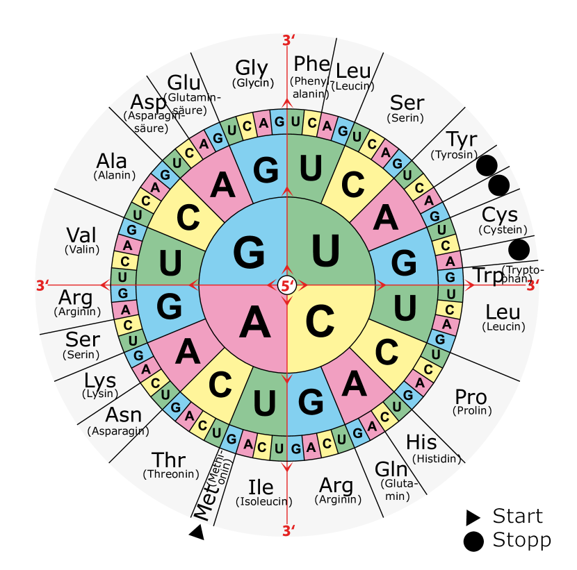
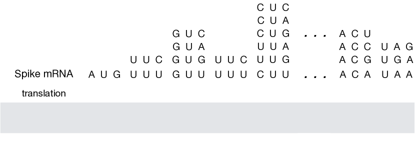
In mRNA design problems, given a target protein sequence $\mathbf{p}=(p_{1},p_{2},...,p_{n})$ where $p_{i}$ denotes the $i$-th amino acid residue, we aim to find a mRNA sequence $\boldsymbol{{x}}=(x_{1},x_{2},..,x_{3n})$ where $x_{i}$ denotes the $i$-th nucleotide, which can be translated to the target protein. During translation, every 3 nucleotides constitute a codon, and each codon specifies a particular amino acid (Figure 2).

It is not hard to see that, for a given target protein, there are exponentially many mRNA sequences which can be translated to the same protein, since an amino acid could potentially be translated from multiple codons. As a result, the number of possible mRNA sequence candidates is the production of the kinds of condons that each amino acid in the given protein sequence can be translated from.

At the meantime, we also hope the designed mRNA sequence $\boldsymbol{{x}}$ satisfies some desired properties (e.g., low minimum free energy) which can be evaluated by the existing computational models. For example, LinearDesign (Zhang et al., 2023) was devised to find the optimal mRNA sequence that has the lowest minimum folding free energy change (MFE) among all feasible mRNA sequences. To write down the formal definition of this optimization problem, we first define a function $\text{MFE}(\boldsymbol{{x}})$ representing the minimum folding free energy change of mRNA x as:

$$\text{MFE}(\boldsymbol{{x}})=\min_{\boldsymbol{{y}}\in\mathcal{Y}(\boldsymbol{{x}})}\Delta G(\boldsymbol{{x}},\boldsymbol{{y}}),$$

where $\mathcal{Y}(\boldsymbol{{x}})$ is the set of all feasible folding structures of mRNA $\boldsymbol{{x}}$, and $\Delta G(\boldsymbol{{x}},\boldsymbol{{y}})$ is a fixed energy model evaluating the free energy change of mRNA $\boldsymbol{{x}}$ and structure $\boldsymbol{{y}}$. This funtion is also known as the RNA folding problem (Huang et al., 2019; Lorenz et al., 2011; Do et al., 2006), where we want to find the most stable structure for the input RNA $\boldsymbol{{x}}$. Based on this function, we can express the optimization problem as:

$$\min\limits_{\boldsymbol{{x}}}\quad \text{MFE}(\boldsymbol{{x}})$$

s.t. $$\boldsymbol{{x}}\in\mathcal{X}(\mathbf{p})$$

where $\mathcal{X}(\mathbf{p})$ is the set of all feasible mRNA sequences encoding protein $\mathbf{p}$. LinearDesign solved this optimization problem in polynomial time via a dynamic programming which utilizes the local decomposable property of $\Delta G(\boldsymbol{{x}},\boldsymbol{{y}})$.

In this paper, we investigate a modified version of the above objective. Instead of finding the mRNA sequence with the lowest $\text{MFE}(\boldsymbol{{x}})$, we aim to find the mRNA with the largest partition function $Q(\boldsymbol{{x}})$. Instead of optimizing the single most stable structure, we want to optimize the stability of all potential folding structures simultaneously, and end up with a much smoother landscape. Formally, we can express the new optimization problem as:

$$\begin{split}\min\limits_{\boldsymbol{{x}}}\quad&-Q(\boldsymbol{{x}})\\ \textrm{s.t.}\quad&\boldsymbol{{x}}\in\mathcal{X}(\mathbf{p})\end{split}$$ (1)

By using this new objective, we can find mRNA sequences with multiple low free energy change conformations, which could potentially lead to more stable designed mRNAs. It turns out that this new optimization formulation is NP-hard, and the orignal algorithm from LinearDesign cannot be extend to efficiently solve this Problem.

Given the complexity of directly optimizing $Q(\boldsymbol{{x}})$, an alternative approach is to approximate this optimization problem by focusing on the expected partition function $\widetilde{Q}(\mathbb{D})$. We propose to optimize $\widetilde{Q}(\mathbb{D})$, which reflects the average stability over a distribution of RNA sequences. This approach simplifies the problem by considering the average behavior rather than the exact configurations of each RNA sequence. The new optimization problem can then be reformulated as:

$$\begin{split}\min\limits_{\mathbb{D}}\quad&-\widetilde{Q}(\mathbb{D})\\ \textrm{s.t.}\quad&\mathbb{D}\text{ is a valid distribution over }\mathsf{N}^{n}\end{split}$$ (2)

In the new formulation, $\widetilde{Q}(\mathbb{D})$ can be efficiently computed via dynamic programming, similar to LinearDesign. This enables the use of gradient-based optimization methods to optimize it.

Building on this foundation, we introduce the ensemble free energy, $\Delta G^{\circ}_{\text{ensemble}}(\boldsymbol{{x}})$, for an individual RNA sequence $\boldsymbol{{x}}$. This metric provides a more holistic view of stability by considering contributions from all competing structures, as opposed to just the Minimum Free Energy (MFE). It is defined as:

$$\Delta G^{\circ}_{\text{ensemble}}(\boldsymbol{{x}})=-RT\log Q(\boldsymbol{{x}}),$$

where $R$ is the universal gas constant, and $T$ is the absolute temperature.

Extending this concept to our previously defined expected partition function, we introduce the generalized ensemble free energy , $\widetilde{\Delta G^{\circ}}_{\text{ensemble}}(\mathbb{D})$. This metric captures the ensemble free energy across the expected distribution of partition functions over all possible RNA sequences. It is formulated as:

$$\widetilde{\Delta G^{\circ}}_{\text{ensemble}}(\mathbb{D})=-RT\log\widetilde{Q}(\mathbb{D}),$$

where $\widetilde{Q}(\mathbb{D})$ represents the expected partition function over the joint distribution of all positions.

Thus, the generalized ensemble free energy offers a measure of the expected stability of an ensemble of RNA sequences, taking into account not only the probabilistic distribution of the sequences but also their potential folding structures.

Following Zhang et al. (2023), we approach the mRNA design problem through lattice parsing. In this model, the RNA sequence is represented as a path through a lattice structure, where each node corresponds to a state in the RNA sequence construction process. To define a distribution over this lattice, we consider not only the per-position distribution of nucleotides but also the transitions between states in the lattice. Each node $q$ in the lattice is associated with a distribution over possible outgoing transitions (edges), which represent the addition of nucleotides at that position.

For each node $q$ in the lattice, define the distribution:

$$\mathbb{D}_{q}:\mathsf{N}(q)\mapsto[0,1],\text{s.t.~{}}\sum_{x\in\mathsf{N}(q)}\mathbb{D}_{q}(x)=1$$

where $\mathsf{N}(q)$ is the set of nucleotides permissible at node $q$, determined by the function $\delta(q,a)$, which defines the valid transitions from node $q$ with nucleotide $a$.

The overall distribution of mRNA sequences in this lattice, denoted as $\mathbb{D}:\mathsf{N}^{n}\mapsto[0,1]$, is thus a product of distributions at each node along the path:

$$\mathbb{D}(\boldsymbol{{x}})=\prod_{i}\mathbb{D}_{q_{i}}(x_{i}),\text{ given $q_{0}=(0,0)$ and $q_{i+1}=\delta(q_{i},x_{i})$},$$

where $q_{0}=(0,0)$ is the starting node, and $q_{i+1}=\delta(q_{i},x_{i})$ is the next node reached by adding nucleotide $x_{i}$.

3.2 Problem 2: Non-coding RNA Design for Maximum Boltzmann Probability

Another rapidly advancing field of study lies in the realm of non-coding RNA design Garcia-Martin et al. (2013); Zadeh et al. (2011); Portela (2018); Zhou et al. (2023), which has profound applications in RNA-based therapeutics and diagnostics. The primary objective of RNA design, dealing with a designated target structure, is to identify a sequence that folds into that structure. Fitness functions commonly employed for non-coding RNA design encompass the Minimum Free Energy (MFE) and Unique Minimum Free Energy (uMFE), necessitating that the designed sequence(s) adopt the target structure as its MFE structure (in a unique manner). However, the problem of RNA design under the MFE or uMFE criterion has been proven to be NP-Hard Bonnet et al. (2020) for base pair based energy models. Additional widely used fitness functions for RNA design include ensemble defect and equilibrium probability, addressing the concern that MFE structure(s), although the most probable structure, might be low probability within the structure ensemble of an RNA sequence. Remarkably, SAMFEO Zhou et al. (2023) demonstrates that optimizing the conditional probability

$$p(\boldsymbol{{y}}\mid\boldsymbol{{x}})=\frac{e^{-\Delta G(\boldsymbol{{x}},\boldsymbol{{y}})/RT}}{Q(\boldsymbol{{x}})}$$

not only enhances the thermodynamic stability of the target structure but also results in a plethora of MFE or uMFE solutions (this $p(\boldsymbol{{y}}\mid\boldsymbol{{x}})$ is also known as the “equilibrium” or “Boltzmann” probability). It is worth noting that if the (equilibrium) probability of the target structure reaches a substantial level, such as $0.5$, the challenge of finding MFE solutions can be reduced to maximizing the probability of the target structure. This is because it becomes impossible for any other structure to possess a probability exceeding $0.5$. Consequently, it is plausible that the task of identifying RNA sequence(s) with optimal probability for the target structure is also a NP-hard problem.

To optimize the conditional probability $p(\boldsymbol{{y}}\mid\boldsymbol{{x}})$ for RNA design, we can maximize its logarithm

$$\max_{\boldsymbol{{x}}}\log[e^{-\Delta G(\boldsymbol{{x}},\boldsymbol{{y}})/RT}/Q(\boldsymbol{{x}})],$$

which is equivalent to

$$\min_{\boldsymbol{{x}}}\Delta G(\boldsymbol{{x}},\boldsymbol{{y}})/RT+\log Q(\boldsymbol{{x}}).$$

With continuous relaxation, we minimize the expectation of the above quantity:

$$\min_{\mathbb{D}}\operatorname{\mathbb{E}}_{\boldsymbol{{x}}\sim\mathbb{D}(\cdot)}[\Delta G(\boldsymbol{{x}},\boldsymbol{{y}})/RT]+\operatorname{\mathbb{E}}_{\boldsymbol{{x}}\sim\mathbb{D}(\cdot)}[\log Q(\boldsymbol{{x}})].$$

The second term can be bounded above by the logarithm of our expected partition function via Jensen’s inequality (swapping the order of $\operatorname{\mathbb{E}}$ and $\log$):

$$\operatorname{\mathbb{E}}_{\boldsymbol{{x}}\sim\mathbb{D}(\cdot)}[\log Q(\boldsymbol{{x}})]\leq\log\operatorname{\mathbb{E}}_{\boldsymbol{{x}}\sim\mathbb{D}(\cdot)}[Q(\boldsymbol{{x}})]=\log\widetilde{Q}(\mathbb{D}).$$

So we actually optimize the following:

$$\min_{\mathbb{D}}\operatorname{\mathbb{E}}_{\boldsymbol{{x}}\sim\mathbb{D}(\cdot)}[\Delta G(\boldsymbol{{x}},\boldsymbol{{y}})/RT]+\log\widetilde{Q}(\mathbb{D}).$$

We can unify this representation by extending the free energy definition to its expected version just like we extended partition function to expected partition function:

$$\widetilde{\Delta G}(\mathbb{D},\boldsymbol{{y}})=\operatorname{\mathbb{E}}_{\boldsymbol{{x}}\sim\mathbb{D}(\cdot)}\Delta G(\boldsymbol{{x}},\boldsymbol{{y}}).$$

Finally the objective can be written as:

$$\min_{\mathbb{D}}\widetilde{\Delta G}(\mathbb{D},\boldsymbol{{y}})+\log\widetilde{Q}(\mathbb{D}).$$ (3)

4 Optimization Methods

In the context of both mRNA and ncRNA design, we aim to optimize a objective function over all valid probability distributions $\mathbb{D}$ for RNA sequences in the design space:

$$\min_{\mathbb{D}:\mathcal{X}\mapsto[0,1]}\ell(\mathbb{D})$$ (4)

In the equation above, we strive to identify the probability distribution $\mathbb{D}$ that yields the minimum value for the objective function $\ell(\mathbb{D})$.

In the sections that follow, we describe two distinct methods to tackle this optimization problem. We first discuss it as a constrained optimization problem in Section 4.1, followed by its interpretation as an unconstrained optimization problem in Section 4.2.

4.1 Method 1: Constrained Optimization via Projected Gradient Descent

One way to define the parameters of the probability distribution $\mathbb{D}$ is by expressing it as the product of individual probabilities, thus:

$$\mathbb{D}_{\boldsymbol{\theta}}(\boldsymbol{{x}})=\prod_{i}\theta_{q_{i},x_{i}}$$

Here, $\theta_{q_{i},x_{i}}$ stands for the probability of selecting the nucleotide $x_{i}$ at the node $q_{i}$ within a lattice, and $\boldsymbol{\theta}$ encompasses all such probabilities for each nucleotide at each node.

The optimization problem can then be formulated as follows:

$$\min_{\boldsymbol{\theta}} \ell(\mathbb{D}_{\boldsymbol{\theta}})$$ (5)

subject to $$\forall q,\sum_{x\in\mathsf{N}(q)}\theta_{q,x}=1$$

In the equation above, we aim to minimize the objective function $\ell(\mathbb{D}_{\boldsymbol{\theta}})$ subject to the constraint that for every node $q$, the sum of the probabilities of each possible nucleotide is equal to 1. This constraint ensures that each set of probabilities $\theta_{q_{i}}$ forms a valid multinomial distribution over the nucleotides.

Projected gradient descent provides a robust solution to the constrained optimization problem. In this method, we first compute the gradient of our objective function, $\ell(\mathbb{D}_{\boldsymbol{\theta}})$, with respect to the parameters $\boldsymbol{\theta}$. The specific form of this gradient relies on the nature of $\ell$. Upon computing the gradient, we update our parameters by stepping in the negative gradient direction:

$$\boldsymbol{\theta}^{\prime}=\boldsymbol{\theta}^{(t)}-\alpha\nabla\ell(\mathbb{D}_{\boldsymbol{\theta}^{(t)}})$$

where $\alpha$ is a learning rate, and $t$ denotes the current iteration.

Next, we need to project $\boldsymbol{\theta}^{\prime}$ back onto the set of valid multinomial distributions. This can be done by projecting the parameters $\boldsymbol{\theta}_{q}$ in each node $q$ back to the probability simplex, which is eqivelant to solve to following problem:

$$\boldsymbol{\theta}_{q}^{(t+1)}=\operatornamewithlimits{\mathrm{argmin}}_{\boldsymbol{\theta}_{q}}\quad \|\boldsymbol{\theta}_{q}-\boldsymbol{\theta}^{\prime}_{q}\|^{2}_{2}$$

subject to $$\sum_{x\in\mathsf{N}(q)}\theta_{q,x}=1,\quad\theta_{q,x}\geq 0,\forall x\in\mathsf{N}$$

The equation above represents the projection of $\boldsymbol{\theta}^{(t+1)}_{q}$ onto the probability simplex, where $\|\cdot\|^{2}_{2}$ denotes the Euclidean norm. The constraints ensure that $\theta_{q}$ is a valid probability distribution over $\mathsf{N}$. The solution to this problem can be efficiently computed using algorithms for simplex projections.

This process of gradient update and projection is repeated until the changes in $\boldsymbol{\theta}$ or the value of the objective function $\ell(\mathbb{D}_{\boldsymbol{\theta}})$ become sufficiently small, which indicates that the solution has converged.

Algorithm 1 below presents a summary of the projected gradient descent method for the constrained optimization problem:

Algorithm 1 Projected Gradient Descent for Constrained Optimization Formulation

Solution $\boldsymbol{\theta}^{*}$ to the optimization problem

Initialize $\boldsymbol{\theta}^{(0)}$ uniformly such that each $\theta_{q_{i},x_{i}}^{(0)}$ is a valid probability distribution

while not converged do

     Compute gradient $\nabla\ell(\mathbb{D}_{\boldsymbol{\theta}^{(t)}})$

     Update $\boldsymbol{\theta}^{(t+1)}=\boldsymbol{\theta}^{(t)}-\alpha\nabla\ell(\mathbb{D}_{\boldsymbol{\theta}^{(t)}})$

     Project $\boldsymbol{\theta}^{(t+1)}$ onto the probability simplex:

     for each $q$ do

         solve the projection problem to update $\theta_{q}^{(t+1)}$      

     Update $t=t+1$

4.2 Method 2: Unconstrained Optimization using Softmax Parametrization

An alternative approach to the optimization problem (4) is to introduce a parametrization that naturally enforces the required constraints, hence converting the problem into an unconstrained optimization. A common choice for this task is the softmax function due to its inherent property of converting a set of real numbers into a valid probability distribution.

We redefine the parameters of the probability distribution $\mathbb{D}$ using the softmax function as follows:

$$\mathbb{D}_{\boldsymbol{\theta}}(\boldsymbol{{x}})=\prod_{i}\frac{\exp(\theta_{q_{i},x_{i}})}{\sum_{x^{\prime}\in\mathsf{N}}\exp(\theta_{q_{i},x^{\prime}})}$$

In this definition, each $\theta_{q_{i},x_{i}}$ can be any real number. The softmax function ensures that the probabilities of all possible nucleotides at each node $q_{i}$ sum up to 1, thus forming a valid multinomial distribution without explicitly imposing this as a constraint.

With this new parametrization, the optimization problem becomes an unconstrained problem:

$$\min_{\boldsymbol{\theta}}\quad\ell(\mathbb{D}_{\boldsymbol{\theta}})$$ (6)

Since the constraints have been naturally embedded into the problem formulation through the softmax function, we can directly apply the vanilla gradient descent algorithm to solve this optimization problem.

The gradient descent update rule remains the same:

$$\boldsymbol{\theta}^{(t+1)}=\boldsymbol{\theta}^{(t)}-\alpha\nabla\ell(\mathbb{D}_{\boldsymbol{\theta}^{(t)}})$$

However, due to the softmax parametrization, the specific form of the gradient $\nabla\ell(\mathbb{D}_{\boldsymbol{\theta}^{(t)}})$ will be different from that in the constrained optimization problem. Therefore, the derivative of the softmax function will play a role when computing the gradient. The iteration continues until the changes in $\boldsymbol{\theta}$ or the value of the objective function $\ell(\mathbb{D}_{\boldsymbol{\theta}})$ become sufficiently small, indicating that the solution has converged.

Algorithm 2 outlines the procedure of this unconstrained optimization approach:

Algorithm 2 Vanilla Gradient Descent for Unconstrained Optimization Formulation

Solution $\boldsymbol{\theta}^{*}$ to the optimization problem

Initialize $\boldsymbol{\theta}^{(0)}$ randomly

while not converged do

     Compute gradient $\nabla\ell(\mathbb{D}_{\boldsymbol{\theta}^{(t)}})$ taking into account the softmax parametrization

     Update $\boldsymbol{\theta}^{(t+1)}=\boldsymbol{\theta}^{(t)}-\alpha\nabla\ell(\mathbb{D}_{\boldsymbol{\theta}^{(t)}})$

     Update $t=t+1$

4.3 Initialization Method

For ncRNA design, we adopted the targeted initialization (Zhou et al., 2023), which simply sets unpaired base as as a and paired bases as $(\text{\sc c},\text{\sc g})$ or $(\text{\sc g},\text{\sc c})$ randomly.

5 Results on mRNA and non-coding RNA Design

5.1 Preliminary Results on mRNA Design

In this section, we device several types of experiment to investigate the differences of two formulations (Problem (5) and (6)) with different commonly-used first-order optimization algorithms. Here we briefly summarize all optimizers that we used in our experiments:

• Projected Gradient (PG) For the constrained formulation (Problem (5)), we first calculate the gradient without considering all constraints, and then project it back to the probability simplex.

• Projected Gradient with Nesterov’s Acceleration (PG-Nesterov)

• Gradient Descent (GD) For the unconstrained formulation (Problem (6)), we can directly optimize the objective by following the direction of the gradient.

• Gradient Descent with Nesterov’s Acceleration (GD-Nesterov)

• Gradient Descent with RMSProp (GD-RMSProp) Since we are dealing with a unconstrained optimization problem, we can use more advanced gradient estimators to accelerate and stabilize the optimization process.

where the first two optimizers can be used for Problem (5) and the remaining three optimizers can be used for Problem (6).

In our study, we carried out random sampling of protein sequences of various lengths. The protein sequences, each denoted by a unique series of amino acid residues, are presented in Table 1.

Table 1: Random protein sequences of varying lengths used in this study.

Length	Protein Sequence (length includes the stop codon “*”)
20	MKWTHKVKWQMDMNEWHQK*
30	MDCLRSISGPSACWINGRFKVALHLICAY*
40	MQIKSLKDDLKGNLMAWFVMFPNKNERWAPYIMRTYQHM*
50	MMMMRGMPNRFGNYMDMLMFLHGTFETTFRVLRPTHEKYKDEIVKDTQW*
60	MEKRPNQGATVVMHCGVCWWTWLFAQVKCSISKYASIDEYNNIATAISMKVQAKFNPQL*
80	MSWVHNHLCDMFTIYFAPWFEWFVMNTRTYWPFDFMRRDSLNAAYNGRNDLPPHQLARGL
	WDWLKTISQMIYHWWNWFL*
100	MGWVCLGTCHMEVHHGCHVQAEIVNVVGTFHPAKSMTFMCIHDCLCFWCCCHSHSGLEND
	YRQDKYCGDANALYLQCPMADPDNQVELETDAWDGDKFH*

5.1.1 Energy Model

In the preliminary experiments, we use a revised Nussinov–Jacobson energy model. For a mRNA $\boldsymbol{{x}}=(x_{1},x_{2},...,x_{m})$ where $x_{i}\in\{\texttt{A},\texttt{C},\texttt{G},\texttt{U}\}$ and a dot-bracket sequence (i.e., folding structure) $\boldsymbol{{y}}=(z_{1},z_{2},...,z_{m})$ where $z_{i}\in\{\texttt{.},\texttt{(},\texttt{)}\}$, “.” denotes an unpaired base and “( )” denotes a paired bases. We assign a free energy change of $\delta(\boldsymbol{{x}},i)$ for an unpaired base at position $i$, and a free energy change of $\xi(\boldsymbol{{x}},i,j)$ for a paired bases at position $i$ and $j$. A very common setting is that $\delta(\boldsymbol{{x}},i)=1\,\mathrm{kcal/mol}$; $\xi(\boldsymbol{{x}},i,j)=-3\,\mathrm{kcal/mol}$ for CG pairs; $\xi(\boldsymbol{{x}},i,j)=-2\,\mathrm{kcal/mol}$ for AU pairs; and $\xi(\boldsymbol{{x}},i,j)=-1\,\mathrm{kcal/mol}$ for GU pairs. The total free energy change can be calculated as:

$$\Delta G(\boldsymbol{{x}},\boldsymbol{{y}})=\sum_{i\in\text{unpaired}(\boldsymbol{{y}})}\delta(\boldsymbol{{x}},i)+\sum_{(i,j)\in\text{pairs}(\boldsymbol{{y}})}\xi(\boldsymbol{{x}},i,j),$$ (7)

where $\text{unpaired}(\boldsymbol{{y}})$ is the set of unpaired bases (specified by “.”), and $\text{paired}(\boldsymbol{{y}})$ is the set of paired bases (specified by “(” and “)”). For example, let’s say we have a mRNA sequence $\boldsymbol{{x}}=``\texttt{AUGCUGUGA}\text{''}$ and a structure $\boldsymbol{{y}}=``\texttt{.(.(...))}\text{''}$. Then, we can calculate $\Delta G(\boldsymbol{{x}},\boldsymbol{{y}})=\delta(\boldsymbol{{x}},1)+\delta(\boldsymbol{{x}},3)+\delta(\boldsymbol{{x}},5)+\delta(\boldsymbol{{x}},6)+\delta(\boldsymbol{{x}},7)+\xi(\boldsymbol{{x}},2,9)+\xi(\boldsymbol{{x}},4,8)=1+1+1+1+1-2-3=0$.

5.1.2 Results and Analysis

Sensitivity to Learning Rate

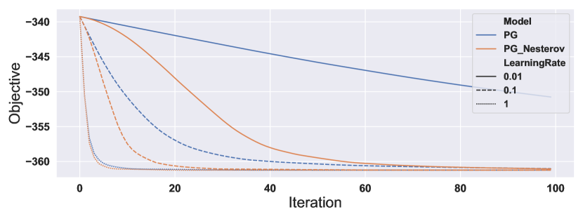
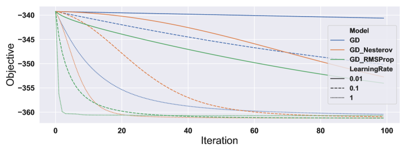
In mRNA vaccines design problems, the design objectives are generally non-convex, and it is hard to directly determine a good learning rate for different optimizers. Ideally, a preferred optimizer can relatively quickly converge to a good local optimum with a wide range of learning rates. Here we tested all 5 optimizers on a target protein of length 100. Figure 3 shows the learning curves for different optimizers with various learning rates, comparing their performance on both constrained and unconstrained formulations.

(a) Learning curves of different optimizers and learning rates on the constrained formulation.

(b) Learning curves of different optimizers and learning rates on the unconstrained formulation.

Figure 3: Comparison of learning curves for different optimizers and learning rates on both constrained (left) and unconstrained (right) formulations. For the constrained formulation, Nesterov’s Acceleration can accelerate the optimization process and converge to a better solution, making it less sensitive to learning rate. For the unconstrained formulation, RMSProp can converge faster than Nesterov’s Acceleration, but it might converge to a suboptimal solution (e.g., LearningRate $=1$).

Speed of Convergence

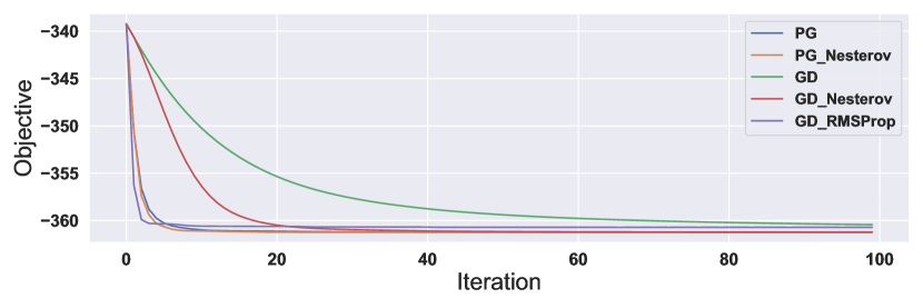
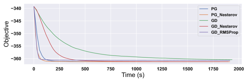
After selecting an appropriate learning rate, we are also interested in the speed of convergence of the optimizers both in terms of iteration and time. Here we plot the learning curve of optimizers with a fixed learning rate on optimizing the same target protein we used before. We can see that PG, PG-Nesterov, and GD-RMSPorp converge significantly faster than GD and GD-Nesterov. However, GD-RMSPorp could converge to a suboptimal solution compared with PG, PG-Nesterov, and GD-Nesterov. Figure 4 illustrates these findings.

(a) “Iteration v.s. Objective” plot of different optimizers.

(b) “Time v.s. Objective” plot of different optimizers.

Figure 4: Comparison of convergence speed of different optimizers in terms of iterations (left) and time (right), with a fixed learning rate (LearningRate $=1$).

Effectiveness on Proteins of Different Length

In Table 2, we compare the final objective value of different optimizers after running a fixed steps of optimization. We sample proteins with different lengths and choose a large enough number of steps so that every optimizer can converge within such iterations. Here we listed the results on the following table. We can observe that PG and PG-Nesterov can generally coverge to a better solution and are robust across different lengths. GD-RMSProp could find a better solution than other optimizers (e.g., in the case of length $=50$), but it’s could also get stuck in a suboptimal solution in many cases. GD-Nesterov can also converge to good solutions in most cases.

Table 2: Final objective value on proteins of different length, after 100 Iterations.
(ensemble free energy change in $\mathrm{kcal/mol}$)

Model	Sample Protein Length
	20	30	40	50	60	80	100
PG	-56.77	-105.39	-135.67	-171.01	-210.75	-283.86	-361.23
PG-Nesterov	-56.77	-105.39	-135.67	-171.02	-210.75	-283.86	-361.23
GD	-56.77	-105.32	-135.67	-170.95	-210.60	-283.48	-361.18
GD-Nesterov	-56.77	-105.39	-135.67	-170.99	-210.60	-283.48	-361.23
GD-RMSProp	-56.77	-105.39	-134.98	-171.11	-210.50	-283.63	-360.72

Comparative Analysis of MFE & EPF Values

In Table 3, we conduct a detailed analysis of Minimum Free Energy (MFE) and Ensemble Partition Function (EPF) values across various optimization models for proteins of different lengths. Despite the varying final performance of each method, it is noteworthy that all the methods outperform the traditional approach that focuses only on optimizing MFE (represented by the LinearDesign model) in finding better $\Delta G^{\circ}_{\text{ensemble}}$ solutions.

Table 3: Final MFE & EPF values on proteins of different length. (Iterations = 100)

Model	Length = 20		Length = 50		Length = 80		Length = 100
	MFE	$\Delta G^{\circ}_{\text{ensemble}}$	MFE	$\Delta G^{\circ}_{\text{ensemble}}$	MFE	$\Delta G^{\circ}_{\text{ensemble}}$	MFE	$\Delta G^{\circ}_{\text{ensemble}}$
LinearDesign	-45.00	-56.25	-151.00	-168.92	-255.00	-281.24	-327.00	-356.14
PG	-44.00	-56.77	-143.00	-171.01	-245.00	-283.86	-310.00	-361.23
PG-Nesterov	-44.00	-56.77	-144.00	-171.02	-245.00	-283.86	-310.00	-361.23
GD	-44.00	-56.77	-145.00	-170.95	-242.00	-283.48	-311.00	-361.18
GD-Nesterov	-44.00	-56.77	-143.00	-170.99	-242.00	-283.48	-310.00	-361.23
GD-RMSProp	-44.00	-56.77	-144.00	-171.11	-245.00	-283.63	-309.00	-360.72

Fractional & Integral Solutions Along the Optimization Process

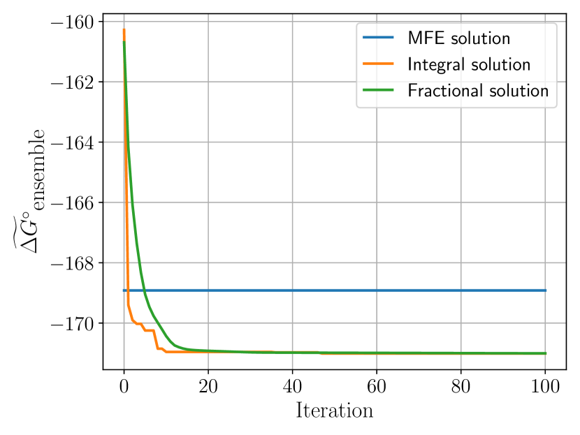
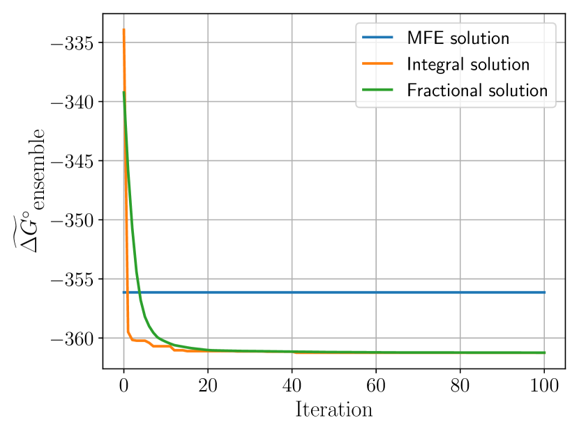
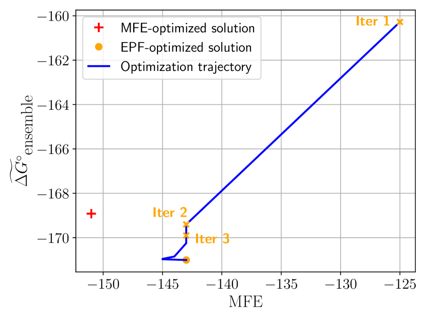
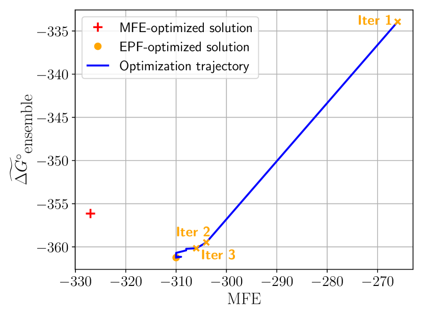
Figures 5 and 6 display the fractional and integral solutions during the optimization process for the protein sequences of length 50 and 100, respectively. In Figure 5, it is evident that, as the optimization progresses, the EPF-optimized solutions converge rapidly and surpass the MFE-optimized solution in terms of the ensemble partition function, indicating the effectiveness of the methods. In Figure 6, the trajectory of the optimization process is visualized, plotting the ensemble free energy against the MFE for each iteration. It highlights the dynamic progress and the explorative path taken by the optimization algorithms, demonstrating their ability to navigate the energy landscape effectively.

(a) Rand 50

(b) Rand 100

Figure 5: Fractional & intergral solutions along the optimization process.

(a) Rand 50

(b) Rand 100

Figure 6: Integral solutions along the optimization process.

5.2 Preliminary Results on non-coding RNA Design

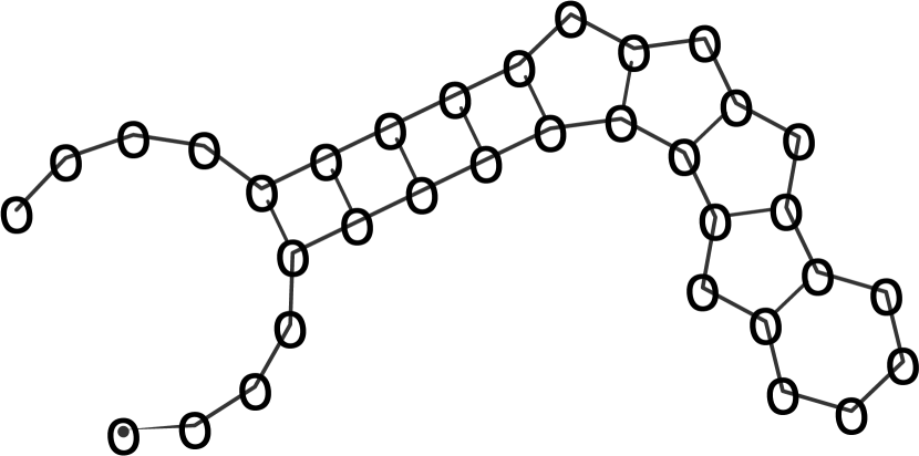
The Eterna100 dataset Anderson-Lee et al. (2016) is a popular benchmark for evaluating RNA design programs, which consists 100 secondary structures (i.e., “puzzles”) of varying design difficulties, spanning from simple hairpins to intricate multiloop structures. For our study, we focused on relatively short structures with a maximum length of 68 nucleotides (28 structures).

In this work, we optimized two objective functions: conditional probability from Equation 3 and expected free energy, $\widetilde{\Delta G}(\mathbb{D},\boldsymbol{{y}})$. Both objective functions are based on the simplified energy model (omitting special hairpins, dangling ends, and special internal loops). After optimization, we then picked the integral solution with the best $p(\boldsymbol{{y}}\mid\boldsymbol{{x}})$ under the full energy model across the gradient descent iterations. Here we use the projected gradient descent method for optimization.

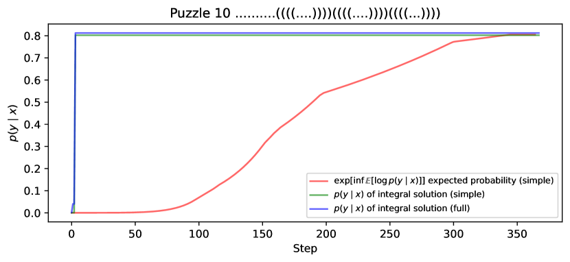
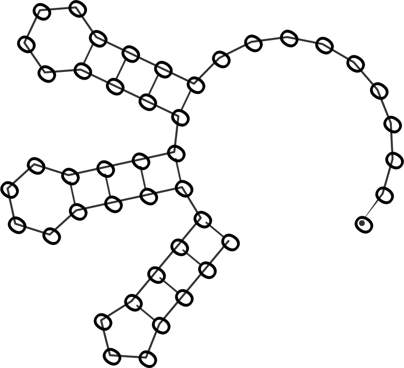
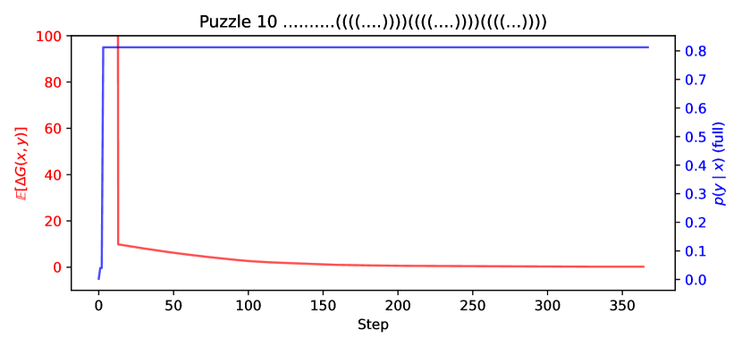
The result is presented in Table 4. Due to the targeted initialization, some puzzles (1, 3, 8, 26, and 30) exhibited a decent initial integral solution with $p(\boldsymbol{{y}}\mid\boldsymbol{{x}})$ over $0.9$. Still, many structures see improvements in $p(\boldsymbol{{y}}\mid\boldsymbol{{x}})$ through the optimization. Notably, Puzzles 10 improved by $0.624$ while Puzzles 33 and 46 by about $.450$. Puzzles 57 and 67 are proved to be undesignable using the 2004 Turner energy model as implemented in the Vienna package Zhou et al. (2024), so it is unlikely to obtain a high $p(\boldsymbol{{y}}\mid\boldsymbol{{x}})$ for them.

Figure 7: Objective optimization of Equation 3 (left) and $\mathbb{E}[\Delta G(\boldsymbol{{x}},\boldsymbol{{y}})]$ (right) for puzzle 10, 23, 40, and 88. The red curve depicts the improvement in objective values across the gradient descent iterations. The green and blue curves represents the $p(\boldsymbol{{y}}\mid\boldsymbol{{x}})$ of the integral solution obtained from the distributions for the simple and full energy model respectively.

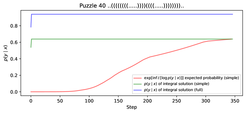
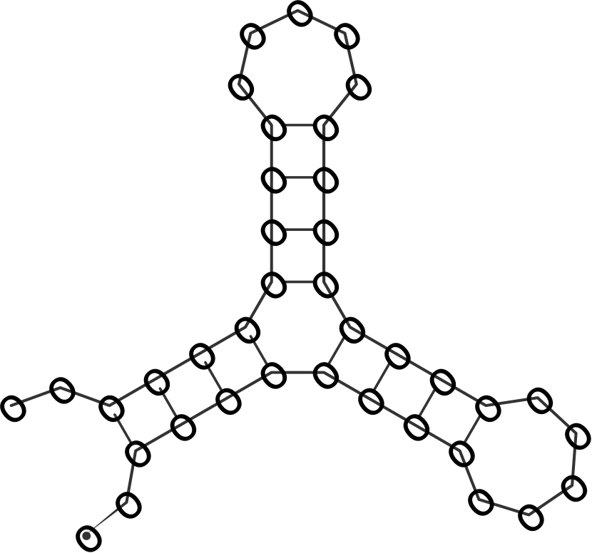
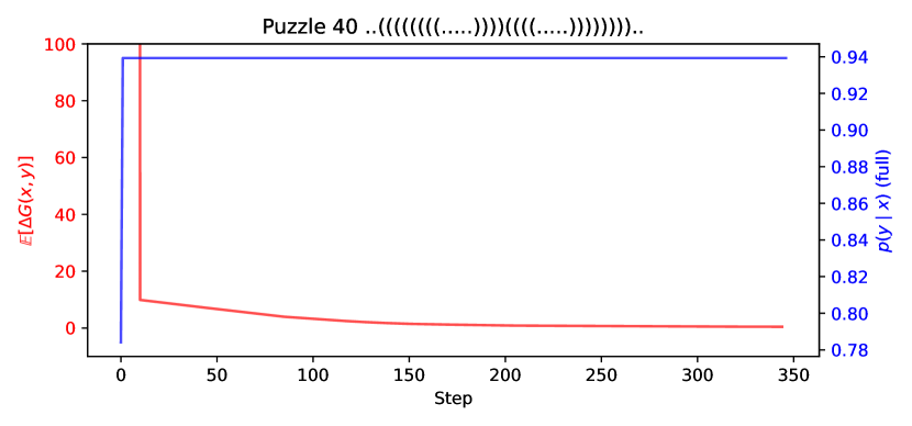
Although optimizing expected free energy is significantly faster than conditional probability, it can be more susceptible to local minima. This is demonstrated by Puzzle 10 and 40, where optimizing conditional probability outperformed optimizing free energy by around $0.150$. After all, minimizing free energy does not account for the partition function $Q(\boldsymbol{{x}})$, meaning that the designed sequence can have many competing structures Kayedkhordeh et al. (2021).

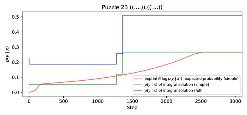
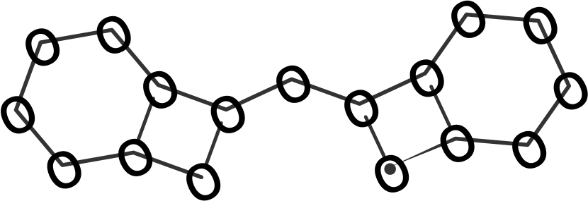
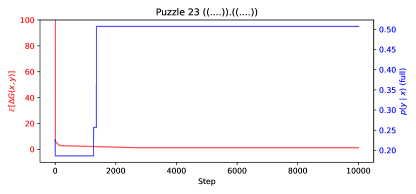
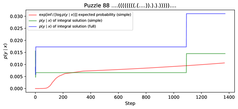
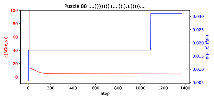
In Figure 7, we visualize the change in objective values for Puzzles 10, 23, 40, and 88. For cases like Puzzles 10 and 40, the integral solution is found early on, while the fractional solution slowly converges into it. Whereas, Puzzles 23 and 88 still see improvements in $p(\boldsymbol{{y}}\mid\boldsymbol{{x}})$ after 1000 steps.

Table 4: Preliminary results for non-coding RNA design on the short structures from the Eterna100 dataset (length up to 70), showing final $p(\boldsymbol{{y}}\mid\boldsymbol{{x}})$ from different methods. Initial: targeted initialization; Simple: $p(\boldsymbol{{y}}\mid\boldsymbol{{x}})$ in the simplified energy model; Full: $p(\boldsymbol{{y}}\mid\boldsymbol{{x}})$ in the full energy model.

			Initial		optimizing		optimizing
					$-\log p(\boldsymbol{{y}}\mid\boldsymbol{{x}})$		$\Delta G(x,y)$	structure
ID	Name	Len.	Simple	Full	Simple	Full	Full
8	G-C Placement	12	0.963	0.948	0.963	0.948	0.948
1	Simple Hairpin	16	0.994	0.975	0.993	0.975	0.976
23	Shortie 4	17	0.045	0.227	0.266	0.507	0.529
26	stickshift	26	0.949	0.955	0.957	0.957	0.984
15	Small and Easy 6	30	0.000	0.000	0.001	0.290	0.395
30	Corner bulge training	31	0.925	0.909	0.942	0.928	0.981
88	Zigzag Semicircle	34	0.016	0.009	0.015	0.031	0.024
41	Shortie 6	35	0.000	0.012	0.000	0.021	0.018
11	InfoRNA test 16	36	0.632	0.849	0.632	0.849	0.922
3	Prion Pseudoknot	36	0.955	0.958	0.952	0.968	0.961
57	multilooping fun	36	0.000	0.000	0.000	0.000	0.000
66	Bug 38	36	0.004	0.001	0.082	0.039	0.014
40	Tripod5	38	0.539	0.784	0.638	0.939	0.784
65	Branching Loop	40	0.000	0.027	0.000	0.396	0.406
20	InfoRNA bulge test 9	42	0.049	0.195	0.274	0.602	0.519
10	Frog Foot	45	0.000	0.002	0.802	0.812	0.626
33	Worm 1	45	0.000	0.000	0.000	0.000	0.448
47	Misfolded Aptamer	50	0.003	0.045	0.001	0.140	0.150
62	Bug 18	53	0.204	0.027	0.204	0.027	0.027
27	U	57	0.035	0.411	0.035	0.411	0.411
67	Simple Single Bond	61	0.006	0.006	0.006	0.006	0.093
25	The Minitsry	62	0.722	0.085	0.722	0.085	0.085
44	An Arm and a Leg 1.0	63	0.013	0.763	0.070	0.778	0.931
45	5 Adj. Stack MultiLoop	63	0.002	0.097	0.002	0.097	0.576
13	square	67	0.887	0.911	0.926	0.945	0.949
18	snoRNA SNORD64	67	0.939	0.895	0.948	0.903	0.970
30	Corner bulge training	67	0.000	0.000	0.000	0.000	0.000
26	stickshift	68	0.178	0.040	0.194	0.117	0.101

6 Related Work

There is a parallel work by Matthies et al. (2023) that also proposes the concept of expected partition function (which they call “structure-sequence partition function”) and also uses continuous optimization for ncRNA design. The major difference is that our work presents a general framework that applies to both mRNA design and ncRNA design.. In fact, we argue that this framework is a better fit for mRNA design than ncRNA design because as Zhang et al. (2023) showed, the mRNA design space can be categorized by a regular language (or finite-state automata) and the objective function (either MFE or partition function) can be formulated as a stochastic context-free grammar (SCFG). It is well-known in formal language theory that the intersection of a (stochastic) context-free language and a regular language is another (stochastic) context-free language, which is the essential reason why Zhang et al. (2023)’s algorithm for MFE-based mRNA design runs in worst-case $O(n^{3})$ time. By contrast, the design space for ncRNA design given a target structure $\boldsymbol{{y}}$ is not a regular, but rather a context-free language, because the paired positions in $\boldsymbol{{y}}$ are correlated (for any pair $(i,j)\in\boldsymbol{{y}}$, $x_{i}x_{j}$ must be pairable; it is straightforward to write a context-free grammar for the set of all possible $\boldsymbol{{x}}$ for $\boldsymbol{{y}}$). Unfortunately, the intersection of two context-free languages are context sensitive, which rules out polynomial-time algorithms. This observation suggests that ncRNA design is fundamentally harder than mRNA design, and this framework is more promising on mRNA design.

In terms of the representation of distribution and its optimization, they only used the softmax formulation (Sec. 4.2) while we used both softmax and direct formulation with projected gradient descent (Sec. 4.1).

Even for ncRNA design problem that both work attempted to solve, there is a critical difference in the objective function formulation, which we detail in the Appendix A.

Finally, there is a minor difference in terms of the implementation details for ncRNA design, theirs is in Python and in the original space (i.e., $(+,\times)$ semiring) which will inevitably suffer from overflowing/underflowing on longer structures, while ours is in C++ (based on the LinearPartition codebase) and in logspace (i.e., $(\oplus_{\log},+)$ semiring) which has the potential of better scalability.

7 Conclusions and Future Work

We described a general framework of continuous optimization for RNA design problems based on the concept of expected partition function which is a generalization of classical partition function to a distribution of sequences. We showed how to use this framework for two important use cases, (a) the mRNA design problem optimizing for partition function (i.e., ensemble free energy), and (b) the non-coding RNA design problem optimizing for conditional probability, with promising preliminary results on both. For future work, we will implement the Turner energy model for mRNA design, and scale up the optimization for ncRNA design using the beam search method from LinearPartition Zhang et al. (2020). For the latter, we will also employ a “coupled variables” approach for the paired positions in the target structure which will collapse the $2\times 4$ variables for a paired position to $6$ pair types and make sure paired positions always take valid choices.

Appendix

Appendix A Comparison of Our Optimization on ncRNA Design with Matthies et al. [2023]

Besides the major differences discussed in Section 6 (e.g., our work targets both mRNA and ncRNA design), here we compare the technical details of the concurrent work by Matthies et al. [2023] and our work on ncRNA design (Section 3.2). For the sake of readability, we use our notations to discuss both their and our work.

Their work optimize a variant of (expected) conditional probability which they define as:

$$p(\boldsymbol{{y}}\mid\mathbb{D}) \stackrel{{\scriptstyle\Delta}}{{=}}\frac{\widetilde{Q}_{\boldsymbol{{y}}}(\mathbb{D})}{\widetilde{Q}(\mathbb{D})}$$ (8)

$$=\frac{\operatorname{\mathbb{E}}_{\boldsymbol{{x}}\sim\mathbb{D}(\cdot)}[e^{-\Delta G(\boldsymbol{{x}},\boldsymbol{{y}})/RT}]}{\operatorname{\mathbb{E}}_{\boldsymbol{{x}}\sim\mathbb{D}(\cdot)}[Q(\boldsymbol{{x}})]},$$ (9)

where $\widetilde{Q}_{\boldsymbol{{y}}}(\mathbb{D})$ is interpreted as the expected sequence partition function, representing the weighted sum of Boltzmann weights for all sequences given the fixed structure $\boldsymbol{{y}}$:

$$\widetilde{Q}_{\boldsymbol{{y}}}(\mathbb{D})=\operatorname{\mathbb{E}}_{\boldsymbol{{x}}\sim\mathbb{D}(\cdot)}[e^{-\Delta G(\boldsymbol{{x}},\boldsymbol{{y}})/RT}]=\sum_{\boldsymbol{{x}}}\mathbb{D}(\boldsymbol{{x}})e^{-\Delta G(\boldsymbol{{x}},\boldsymbol{{y}})/RT}.$$ (10)

However, it is critical to understand that the objective they proposed differs from the original goal of ncRNA design, which was to optimize:

$$\operatorname{\mathbb{E}}_{\boldsymbol{{x}}\sim\mathbb{D}(\cdot)}[p(\boldsymbol{{y}}\mid\boldsymbol{{x}})]=\operatorname{\mathbb{E}}_{\boldsymbol{{x}}\sim\mathbb{D}(\cdot)}\left[\frac{e^{-\Delta G(x,y)/RT}}{Q(x)}\right]{\color[rgb]{1,0,0}\neq\frac{\operatorname{\mathbb{E}}_{\boldsymbol{{x}}\sim\mathbb{D}(\cdot)}[e^{-\Delta G(\boldsymbol{{x}},\boldsymbol{{y}})/RT}]}{\operatorname{\mathbb{E}}_{\boldsymbol{{x}}\sim\mathbb{D}(\cdot)}[Q(\boldsymbol{{x}})]}\stackrel{{\scriptstyle\Delta}}{{=}}p(y\mid\mathbb{D})}.$$ (11)

The discrepancy is due to the fact that the expectation of a fraction is not the fraction of expectations.

In our work, we directly optimize the expected logarithm of conditional probability:

$$\operatorname{\mathbb{E}}_{\boldsymbol{{x}}\sim\mathbb{D}(\cdot)}[\log p(\boldsymbol{{y}}\mid\boldsymbol{{x}})] =\operatorname{\mathbb{E}}_{\boldsymbol{{x}}\sim\mathbb{D}(\cdot)}\left[\log\left(\frac{e^{-\Delta G(\boldsymbol{{x}},\boldsymbol{{y}})/RT}}{Q(\boldsymbol{{x}})}\right)\right].$$ (12)

Given the complexities in directly optimizing this objective, our proposal includes optimizing a lower bound:

$$\operatorname{\mathbb{E}}_{\boldsymbol{{x}}\sim\mathbb{D}(\cdot)}[\log p(\boldsymbol{{y}}\mid\boldsymbol{{x}})] =\operatorname{\mathbb{E}}_{\boldsymbol{{x}}\sim\mathbb{D}(\cdot)}\left[\log\left(\frac{e^{-\Delta G(\boldsymbol{{x}},\boldsymbol{{y}})/RT}}{Q(\boldsymbol{{x}})}\right)\right]$$ (13)

$$=\operatorname{\mathbb{E}}_{\boldsymbol{{x}}\sim\mathbb{D}(\cdot)}[-\Delta G(\boldsymbol{{x}},\boldsymbol{{y}})/RT-\log Q(\boldsymbol{{x}})]$$ (14)

$$=-\operatorname{\mathbb{E}}_{\boldsymbol{{x}}\sim\mathbb{D}(\cdot)}[\Delta G(\boldsymbol{{x}},\boldsymbol{{y}})/RT]-\operatorname{\mathbb{E}}_{\boldsymbol{{x}}\sim\mathbb{D}(\cdot)}[\log Q(\boldsymbol{{x}})]$$ (15)

$$\geq-\operatorname{\mathbb{E}}_{\boldsymbol{{x}}\sim\mathbb{D}(\cdot)}[\Delta G(\boldsymbol{{x}},\boldsymbol{{y}})/RT]-{\color[rgb]{1,0,0}\log\operatorname{\mathbb{E}}_{\boldsymbol{{x}}\sim\mathbb{D}(\cdot)}[Q(\boldsymbol{{x}})]},$$ (16)

where the inequality applies Jensen’s Inequality to the log-expectation term.

In contrast, Matthies et al. [2023] directly optimized the logarithm of the expected probability without further simplification:

$$\log p(\boldsymbol{{y}}\mid\mathbb{D}) =\log\left(\frac{\operatorname{\mathbb{E}}_{\boldsymbol{{x}}\sim\mathbb{D}(\cdot)}[e^{-\Delta G(\boldsymbol{{x}},\boldsymbol{{y}})/RT}]}{\operatorname{\mathbb{E}}_{\boldsymbol{{x}}\sim\mathbb{D}(\cdot)}[Q(\boldsymbol{{x}})]}\right)$$ (17)

$$=\log\operatorname{\mathbb{E}}_{\boldsymbol{{x}}\sim\mathbb{D}(\cdot)}[e^{-\Delta G(\boldsymbol{{x}},\boldsymbol{{y}})/RT}]-\log\operatorname{\mathbb{E}}_{\boldsymbol{{x}}\sim\mathbb{D}(\cdot)}[Q(\boldsymbol{{x}})].$$ (18)

However, if we apply Jensen’s Inequality to the first term of their equation, we will arrive at the same lower bound as our proposal:

$$\log p(\boldsymbol{{y}}\mid\mathbb{D}) \geq{\color[rgb]{1,0,0}\operatorname{\mathbb{E}}_{\boldsymbol{{x}}\sim\mathbb{D}(\cdot)}[\log e^{-\Delta G(\boldsymbol{{x}},\boldsymbol{{y}})/RT}]}-\log\operatorname{\mathbb{E}}_{\boldsymbol{{x}}\sim\mathbb{D}(\cdot)}[Q(\boldsymbol{{x}})]$$ (19)

$$=-\operatorname{\mathbb{E}}_{\boldsymbol{{x}}\sim\mathbb{D}(\cdot)}[\Delta G(\boldsymbol{{x}},\boldsymbol{{y}})/RT]-\log\operatorname{\mathbb{E}}_{\boldsymbol{{x}}\sim\mathbb{D}(\cdot)}[Q(\boldsymbol{{x}})].$$ (20)

References

- Anderson-Lee et al. [2016] Jeff Anderson-Lee, Eli Fisker, Vineet Kosaraju, Michelle Wu, Justin Kong, Jeehyung Lee, Minjae Lee, Mathew Zada, Adrien Treuille, and Rhiju Das. Principles for predicting RNA secondary structure design difficulty. Journal of molecular biology, 428(5):748–757, 2016.
- Baden et al. [2021] Lindsey R Baden, Hana M El Sahly, Brandon Essink, Karen Kotloff, Sharon Frey, Rick Novak, David Diemert, Stephen A Spector, Nadine Rouphael, C Buddy Creech, et al. Efficacy and safety of the mRNA-1273 SARS-CoV-2 vaccine. New England Journal of Medicine, 384(5):403–416, 2021.
- Bonnet et al. [2020] Édouard Bonnet, Pawel Rzazewski, and Florian Sikora. Designing RNA secondary structures is hard. Journal of Computational Biology, 27(3):302–316, 2020.
- Cohen and Skiena [2003] Barry Cohen and Steven Skiena. Natural selection and algorithmic design of mRNA. Journal of Computational Biology, 10(3-4):419–432, 2003.
- Crick [1970] Francis Crick. Central dogma of molecular biology. Nature, 227(5258):561–563, 1970.
- Do et al. [2006] Chuong B. Do, Daniel A. Woods, and Serafim Batzoglou. Contrafold: RNA secondary structure prediction without physics-based models. In Proceedings 14th International Conference on Intelligent Systems for Molecular Biology 2006, Fortaleza, Brazil, August 6-10, 2006, pages 90–98, 2006. doi: 10.1093/bioinformatics/btl246. URL https://doi.org/10.1093/bioinformatics/btl246.
- Doudna and Cech [2002] Jennifer A Doudna and Thomas R Cech. The chemical repertoire of natural ribozymes. Nature, 418(6894):222–228, 2002.
- Eddy [2001] Sean R Eddy. Non–coding rna genes and the modern rna world. Nature Reviews Genetics, 2(12):919–929, 2001.
- Garcia-Martin et al. [2013] Juan Antonio Garcia-Martin, Peter Clote, and Ivan Dotu. RNAiFOLD: a constraint programming algorithm for RNA inverse folding and molecular design. Journal of bioinformatics and computational biology, 11(02):1350001, 2013.
- Huang et al. [2019] Liang Huang, He Zhang, Dezhong Deng, Kai Zhao, Kaibo Liu, David A. Hendrix, and David H. Mathews. LinearFold: linear-time approximate RNA folding by 5’-to-3’ dynamic programming and beam search. Bioinformatics, 35(14):i295–i304, 2019. doi: 10.1093/bioinformatics/btz375. URL https://doi.org/10.1093/bioinformatics/btz375.
- Kayedkhordeh et al. [2021] Mohammad Kayedkhordeh, Ryota Yamagami, Philip C. Bevilacqua, and David H. Mathews. Inverse rna folding workflow to design and test ribozymes that include pseudoknots. Methods in molecular biology, 2167:113–143, 2021. URL https://api.semanticscholar.org/CorpusID:220796617.
- Lorenz et al. [2011] Ronny Lorenz, Stephan H. Bernhart, Christian Höner zu Siederdissen, Hakim Tafer, Christoph Flamm, Peter F. Stadler, and Ivo L. Hofacker. Viennarna package 2.0. Algorithms Mol. Biol., 6:26, 2011. doi: 10.1186/1748-7188-6-26. URL https://doi.org/10.1186/1748-7188-6-26.
- Matthies et al. [2023] Marco Matthies, Ryan Krueger, Andrew Torda, and Max Ward. Differentiable Partition Function Calculation for RNA. Nucleic Acids Research, 2023.
- Mauger et al. [2019] David M Mauger, B Joseph Cabral, Vladimir Presnyak, Stephen V Su, David W Reid, Brooke Goodman, Kristian Link, Nikhil Khatwani, John Reynders, Melissa J Moore, et al. mRNA structure regulates protein expression through changes in functional half-life. Proceedings of the National Academy of Sciences, 116(48):24075–24083, 2019.
- McCaskill [1990] J. S. McCaskill. The equilibrium partition function and base pair probabilities for RNA secondary structure. Biopolymers, 29:1105–19, 1990.
- Polack et al. [2020] Fernando P Polack, Stephen J Thomas, Nicholas Kitchin, Judith Absalon, Alejandra Gurtman, Stephen Lockhart, John L Perez, Gonzalo Pérez Marc, Edson D Moreira, Cristiano Zerbini, et al. Safety and efficacy of the BNT162b2 mRNA Covid-19 vaccine. New England journal of medicine, 383(27):2603–2615, 2020.
- Portela [2018] Fernando Portela. An unexpectedly effective Monte Carlo technique for the RNA inverse folding problem. BioRxiv, page 345587, 2018.
- Terai et al. [2016] Goro Terai, Satoshi Kamegai, and Kiyoshi Asai. CDSfold: an algorithm for designing a protein-coding sequence with the most stable secondary structure. Bioinformatics, 32(6):828–834, 2016.
- Wikipedia [2023] Wikipedia. DNA and RNA codon tables. 2023. URL https://en.wikipedia.org/wiki/DNA_and_RNA_codon_tables#/media/File:Aminoacids_table.svg. Wikipedia, The Free Encyclopedia.
- Wu et al. [2020] Fan Wu, Su Zhao, Bin Yu, Yan-Mei Chen, Wen Wang, Zhi-Gang Song, Yi Hu, Zhao-Wu Tao, Jun-Hua Tian, Yuan-Yuan Pei, et al. A new coronavirus associated with human respiratory disease in china. Nature, 579(7798):265–269, 2020.
- Zadeh et al. [2011] Joseph N Zadeh, Brian R Wolfe, and Niles A Pierce. Nucleic acid sequence design via efficient ensemble defect optimization. Journal of computational chemistry, 32(3):439–452, 2011.
- Zhang et al. [2020] He Zhang, Liang Zhang, David H Mathews, and Liang Huang. LinearPartition: linear-time approximation of RNA folding partition function and base-pairing probabilities. Bioinformatics, 36(Supplement_1):i258–i267, 2020.
- Zhang et al. [2023] He Zhang, Liang Zhang, Ang Lin, Congcong Xu, Ziyu Li, Kaibo Liu, Boxiang Liu, Xiaopin Ma, Fanfan Zhao, Huiling Jiang, Chunxiu Chen, Haifa Shen, Hangwen Li, David H. Mathews, Yujian Zhang, and Liang Huang. Algorithm for optimized mRNA design improves stability and immunogenicity. Nature, 621(7978):396–403, 2023. ISSN 1476-4687. doi: 10.1038/s41586-023-06127-z. URL https://doi.org/10.1038/s41586-023-06127-z.
- Zhou et al. [2023] Tianshuo Zhou, Ning Dai, Sizhen Li, Max Ward, David H Mathews, and Liang Huang. RNA design via structure-aware multifrontier ensemble optimization. Bioinformatics, 39(Supplement_1):i563–i571, 2023.
- Zhou et al. [2024] Tianshuo Zhou, Wei Yu Tang, David H. Mathews, and Liang Huang. Undesignable RNA Structure Identification via Rival Structure Generation and Structure Decomposition. To appear in Proceedings of RECOMB 2024, 2024. URL https://arxiv.org/pdf/2311.08339.pdf.