In-Plane Magnon Valve Effect in Magnetic Insulator/Heavy Metal/ Magnetic Insulator Device
Abstract
We propose an in-plane magnon valve (MV), a sandwich structure composed of ferromagnetic insulator/heavy metal/ferromagnetic insulator (MI/HM/MI). When the magnetizations of the two MI layers are parallel, the longitudinal conductance in the HM layer is greater than that in the antiparallel state according to the magnetic proximity effect, termed as the in-plane magnon valve effect. We investigate the dependence of MV ratio (MVR), which is the relative change in longitudinal conductance between the parallel and antiparallel MV states, on the difference in electronic structure between magnetized and non-magnetized metal atoms, revealing that MVR can reach 100%. Additionally, the dependence of MVR on the thickness of metal layer is analyzed, revealing an exponential decrease with increasing thickness. Then we investigate the dependence of HM layer conductance on the relative angle between the magnetizations of two MI layers, illustrating the potential of MV as a magneto-sensitive magnonic sensor. We also investigate the effect of Joule heating on the measurement signal based on the spin Seebeck effect. Two designed configurations are proposed according to whether the electron current is parallel or perpendicular to the magnetization of the MI layer. In the parallel configuration, the transverse voltage differs between the parallel and antiparallel MV states. While in the perpendicular configuration, the longitudinal resistance differs. Quantitative numerical results indicate the feasibility of detecting a voltage signal using the first configuration in experiments. Our work contributes valuable insights for the design, development and integration of magnon devices.
Magnon valve (MV) is a sandwich structure consisting of ferromagnetic insulator/heavy metal/ferromagnetic insulator (MI/HM/MI), which provides a powerful platform for controlling the transport of magnon current [1, 2, 3]. Similar to spin valve [4, 5], which modulates resistance by manipulating the relative magnetization of the magnetic layers, MV can also modulate output magnon current by manipulating the relative magnetization of the magnetic layers. The parallel-state of MV facilitates magnon transmission while its antiparallel-state impedes it, which is called MV effect (MVE) [1]. Due to the advantages of magnon, such as the absence of Joule heat during transport and the prospective development in microwave devices within the GHz-THz frequency band [6, 7, 8, 9, 10, 11, 12, 13, 14, 15, 16], MV has potential to serve as foundational components in the future information technology. Investigation of magnon transport in MV is pivotal for further practical applications of magnon devices. Despite numerous studies on MV manipulation and the fabrication of various structures [3, 2, 1, 17, 18, 19, 20], limitations of transport damping and low conversion ratios constrain their utility.
In experiment, the MV serves to control the activation and deactivation of magnon channels, which necessitates real-time detection of the magnetizations of two MI layers. Typically, two methods are employed to achieve this goal. The first method is to use a magnetic measurement instrument to measure the average magnetization of the MV, such as vibration magnetometer method, which is not compatible with integrated processes. The second method is to deposit a layer of HM onto the MV to detect transmitted magnon currents using the inverse spin Hall effect (ISHE) [1]. However, due to the limited conversion efficiency from spin current to electron current, the ISHE signals measured experimentally for both antiparallel and parallel MV typically exhibit magnitudes on the order of microvolts [1]. The observed signal magnitude is very small, and the measured signal is also susceptible to ambient temperature, which hinder its practical application. Therefore, it is necessary to develop an approach that meets the requirements of integration, has high detection efficiency, robust to environment and enables all-electrical measurement of the relative orientation of magnetizations of MI layers in the MV under external magnetic field.
In this work, we propose a method to determining the relative orientation of magnetizations in two MI layers by measuring the conductance of the middle HM layer in MV. When the magnetizations of the two MI layers are parallel, the longitudinal conductance in the HM layer is greater than that in the antiparallel state due to the magnetic proximity effect (MPE). We analyze the dependence of MV ratio (, where and are longitudinal conductance of metal layer in parallel and antiparallel MV states, respectively) on the difference in electronic structure between magnetized and non-magnetized metal layer atoms. Additionally, we investigate the relationship between and the thickness of the metal layer. Then we investigate the influence of Joule heating on the measurement signal based on the spin Seebeck effect (SSE).
The schematic illustrating the in-plane MV effect (IMVE) based on the MPE is presented in Fig. 1. The MV consists of three components: the upper and lower MI layers are composed of yttrium iron garnet (YIG) with in-plane magnetization, and the central HM layer is composed of platinum (Pt).
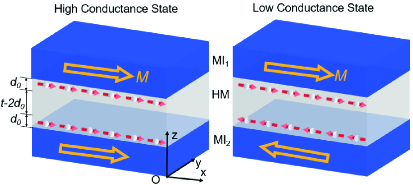
Due to the MPE [21, 22, 23], the electronic structures of Pt atoms in the vicinity of the YIG interfaces are modified. Some Pt atoms undergo a transition from paramagnetic to ferromagnetic states, aligning their magnetic moments with those of the adjacent YIG. We assume the average magnetic moment of Pt atom [21, 22], where is magnetic moment of Pt atoms at YIG/Pt interface, is the distance from the Pt atom to the nearest YIG layer interface and is characteristic length of the MPE. There are two factors which cause to be negatively correlated with : firstly, the proportion of magnetized Pt atoms decreases with increasing ; secondly, the magnetic moments of individual magnetized Pt atoms also decrease with increasing . So far, neither experimental nor first-principles calculations have provided the contribution proportion of these two components. Here, we make a simplified assumption that both factors equally influence the decay of the average magnetic moment of Pt atoms. Although this assumption may slightly deviate from reality, it does not affect the qualitative results. In our calculation, we consider the magnetic moments of unmagnetized and magnetized Pt atoms as follows: , where is Bohr magneton, nm [21]. The proportion of magnetized Pt atoms is , where is the number of magnetized Pt atoms at the YIG/Pt interface. When the thickness of Pt , we can divide the Pt layer into three parts: two magnetization layers at the top and bottom, and an unmagnetized layer in between. Therefore, the Pt layer is analog to a spin valve with a ferromagnet/metal/ferromagnet sandwich configuration. The alteration in YIG magnetic state leads to a variation in the resistance of Pt layer. In the parallel state, the Pt layer exhibits high conductance, while in the antiparallel state, the Pt layer exhibits low conductance.
Here we use the coherent potential approximation (CPA) [24, 25, 26] to calculate the conductance of the Pt layer. The CPA is a well-established method for calculating the conductance of binary alloys [25, 26]. We treat the magnetized Pt atoms and non-magnetized Pt atoms as two distinct atoms coexisting in the Pt layer.
Using the tight binding approximation model, the Hamiltonian of the Pt layer electronic system has the form
| (1) |
Where is the creation (annihilation) operator for electrons with spin s at the i-th layer, and are on-site energy and nearest transition energy, denotes sum over the nearest lattice point.
The on-site energy at the n-th layer takes values and with probabilities and respectively, where is the proportion of magnetized Pt atoms at the n-th layer, is the transition energy. Using the coherent potential, we can calculate the conductance of Pt [24, 25, 27]
| (2) |
where and are the nuclear potential energy and the electron-electron Coulomb interaction energy in magnetized (unmagnetized) Pt atoms, and are the number of outermost electrons and the atomic magnetic moment in the n-th layer of magnetized (unmagnetized) Pt atoms. is the local density of states for electrons with spin s in the n-th layer.
| Parameters | Symbol | Value |
|---|---|---|
| Magnetized atoms’ magnetic moment | 0.2 [21] | |
| Characteristic length of the MPE | 0.4 nm [21] | |
| Gilbert damping constant of YIG | 0.001 [28] | |
| Electrons and magnons coupling | 8 [29] | |
| On-site energy of YIG | 1 eV [9, 30, 31] | |
| Nearest neighbor transition energy | -0.4 eV [9, 30, 31] | |
| Spin Hall angle of Pt | 0.01 [32] | |
| Conductivity of Pt | [33] | |
| Spin diffusion length of Pt | 1.5 nm [34] | |
| Length of Pt | 100 m | |
| Width of Pt | 10 m | |
| Thickness of Pt | 2 nm | |
| Real part of spin mixing conductance | [35] |
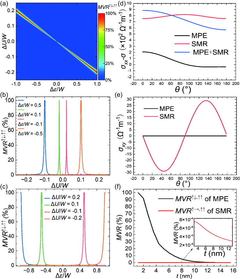
The dependence of on the difference of nuclear potential energy and electron-electron Coulomb interaction energy between magnetized and non-magnetized Pt atoms is shown in Fig. 2(a). The parameters used in calculation are displayed in Table I. By choosing suitable nuclear potential energy and Coulomb interaction, the theoretical of the MV can reach 100%, even comparable to the giant or tunneling magnetoresistance (GMR or TMR). We can see from Eq. (2) that affects the . Because the number of electrons in the outermost layer of Pt is , when is larger, the conductance difference between parallel and antiparallel state is larger. Therefore, the slope corresponding to the maximum is , which is consistent with the calculation result shown by the oblique line in Fig. 2 (a) and peak in Fig. 2 (b, c). The MV also has potential to serve as a magnetic field sensor. We assume that both the applied current and the magnetization of the bottom YIG layer are along the x direction, and the magnetization of the top YIG layer deviate from x direction. When is changed, on the one hand, the magnetization of the magnetized Pt atoms adjacent to the top YIG-Pt interface are changed due to the MPE, and on the other hand, the conductance in Pt layer is changed due to the spin Hall magnetoresistance (SMR) effect [35], the dependence of longitudinal and transverse conductance is shown in Eq. (3) (see Supplementary Material for the detailed derivation).
The dependence of the longitudinal and transverse conductance is shown in Fig. 2 (d, e), the sum conductanceis . We can see that the longitudinal conductance remains the same for and 180°- states when only SMR is considered, but when MPE is present, we can distinguish the two states by only measuring the . And these two states can also be distinguished by measuring transvers conductance , as shown in Fig. 2(e). Finally, we calculate the induced by MPE and induced by SMR as a function of the thickness of the Pt layer under the condition of = -0.528 and = 0.1035, as shown in Fig. 2(f), where is longitudinal conductance when the magnetization of top YIG layer is along y direction and the magnetization of bottom YIG layer is along x direction, is the energy band width. The result demonstrates that as increases, the MVR exhibits an exponential decay.
| (3) |
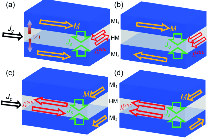
The Joule heating induced by the electron current in the Pt layer will create a temperature gradient between the Pt layer and YIG layer. The temperature gradient, in turn, induces a magnon current that permeates the Pt layer, consequently influencing electron transport in the Pt layer due to ISHE. More specifically, When the current direction is aligned with the magnetization of the YIG layer, as depicted in Fig. 3(a, b). According to the relationship between the ISHE current and the spin current , we can deduce that the spin current will give rise to an transverse ISHE voltage. On the other hand, when the direction of the electron current and magnetization are perpendicular, as depicted in Fig. 3(c, d). Employing a similar analysis to the previous scenario, we can conclude that a temperature gradient will influence the longitudinal resistance.
To further quantify the effect of temperature gradient on the electrical transport properties of the Pt layer, we set the upper and lower YIG layers with temperature , and a middle Pt layer with temperature , where . Considering the nearest neighbor Heisenberg exchange interaction, the Hamiltonian describing the magnon system in the top YIG layer interface is
| (4) |
Where is on-site energy, is the nearest neighbor transition energy, represents the sum over the neighboring lattice sites. Then we can use non equilibrium Green’s method to calculate the magnon current injected from YIG layers to Pt layer [17, 29] (see Supplementary Material for the detailed derivation).
The inverse spin Hall voltage along the y direction is calculated according to the formula.
| (5) |
where is the resistivity of Pt layer, , , is the length, thickness and width of the Pt layer respectively. [32, 36] is the inverse spin Hall electric current, where is spin Hall angle of Pt, is spin diffusion length of Pt, is magnon current injected from YIG layers. The parameters used in simulation are displayed in Table I.
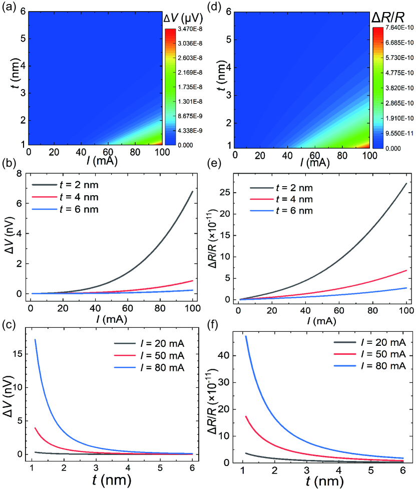
Here we calculate the relationship between current , Pt layer thickness , and the transverse voltage difference between parallel and antiparallel state, depicted in Fig. 4(a). The ambient temperature is 300 K, the results at different ambient temperatures is also calculated (see Supplementary Material for the detail). As increases and the decreases, the temperature gradient generated by the current in the Pt layer increases, therefore generated by the SSE increases. We extract the relationship between , and , which is shown in Fig. 4(b, c). We can see that when reaches 100 mA, it is feasible to generate a measurable voltage up to the magnitude of nV. In the second configuration, we calculate the relationship between longitudinal resistance change rate and , , as shown in Fig. 4(d). We also extract the relationship between the and , and showed in Fig. 4(e, f). increases as increases and decreases, but the relative change is small (on the order of ). Therefore, measuring in experiments poses considerable challenges. Fig. 4(b, c, e, f) demonstrates that both and display an approximat quadratic relationship with respect to and are inversely proportional to . This can be attributed to the direct proportionality of the heat produced by , thereby generating a temperature gradient that is also proportional to and inversely proportional to . Furthermore, the signal induced by the SSE is also proportional to and inversely proportional to .
In this work, we propose the IMVE based on the MPE. We conduct a theoretical investigation into the dependence of on the difference of electron structure between magnetized and non-magnetized Pt atoms. It is found that can reach 100% theoretically. Furthermore, we study the relationship between and the thickness of the Pt layer, revealing an exponential decay as the thickness increases. The dependence of Pt layer conductance on the relative angle between the magnetizations of two MI layers is also calculated, illustrating the potential of MV as a magneto-sensitive magnonic sensor. The influence of Joule heating on the measurement signal based on the SSE is also explored. Two designed configurations are proposed according to whether the electron current is parallel or perpendicular to the magnetization of the MI layer. In the parallel configuration, the transverse voltage differs between the parallel and antiparallel MV states. While in the perpendicular configuration, the longitudinal resistance differs. Quantitative numerical results indicate that it is feasible to measure the voltage signal using the first configuration. Our work contributes valuable insights for the design, development and integration of magnon devices.
This work is financially supported by the National Key Research and Development Program of China (MOST) (Grants No. 2022YFA1402800), the National Natural Science Foundation of China (NSFC) (Grants No. 51831012, 12134017, 11974398), and partially supported by the Strategic Priority Research Program (B) [Grant No. XDB33000000, Youth Innovation Promotion Association of CAS (2020008)].
References
- Wu et al. [2018] H. Wu, L. Huang, C. Fang, B. S. Yang, C. H. Wan, G. Q. Yu, J. F. Feng, H. X. Wei, and X. F. Han, Magnon valve effect between two magnetic insulators, Physical Review Letters 120, 097205 (2018).
- Cramer et al. [2018] J. Cramer, F. Fuhrmann, U. Ritzmann, V. Gall, T. Niizeki, R. Ramos, Z. Qiu, D. Hou, T. Kikkawa, J. Sinova, U. Nowak, E. Saitoh, and M. Kläui, Magnon detection using a ferroic collinear multilayer spin valve, Nature Communications 9, 1089 (2018).
- Cornelissen et al. [2018] L. J. Cornelissen, J. Liu, B. J. van Wees, and R. A. Duine, Spin-current-controlled modulation of the magnon spin conductance in a three-terminal magnon transistor, Physical Review Letters 120, 097702 (2018).
- Baibich et al. [1988] M. N. Baibich, J. M. Broto, A. Fert, F. N. Van Dau, F. Petroff, P. Etienne, G. Creuzet, A. Friederich, and J. Chazelas, Giant Magnetoresistance of (001)Fe/(001)Cr Magnetic Superlattices, Physical Review Letters 61, 2472 (1988).
- Binasch et al. [1989] G. Binasch, P. Grünberg, F. Saurenbach, and W. Zinn, Enhanced magnetoresistance in layered magnetic structures with antiferromagnetic interlayer exchange, Physical Review B 39, 4828 (1989).
- Mathieu et al. [2003] C. Mathieu, V. T. Synogatch, and C. E. Patton, Brillouin light scattering analysis of three-magnon splitting processes in yttrium iron garnet films, Phys. Rev. B 67, 104402 (2003).
- Serga et al. [2010] A. A. Serga, A. V. Chumak, and B. Hillebrands, YIG magnonics, Journal of Physics D: Applied Physics 43, 264002 (2010).
- Vogel et al. [2015] M. Vogel, A. V. Chumak, E. H. Waller, T. Langner, V. I. Vasyuchka, B. Hillebrands, and G. von Freymann, Optically reconfigurable magnetic materials, Nature Physics 11, 487 (2015).
- Barker and Bauer [2016a] J. Barker and G. E. W. Bauer, Thermal spin dynamics of yttrium iron garnet, Phys. Rev. Lett. 117, 217201 (2016a).
- Chumak et al. [2017] A. V. Chumak, A. A. Serga, and B. Hillebrands, Magnonic crystals for data processing, Journal of Physics D: Applied Physics 50, 244001 (2017).
- Lu et al. [2017] J. Lu, X. Li, H. Y. Hwang, B. K. Ofori-Okai, T. Kurihara, T. Suemoto, and K. A. Nelson, Coherent two-dimensional terahertz magnetic resonance spectroscopy of collective spin waves, Phys. Rev. Lett. 118, 207204 (2017).
- Barker and Bauer [2019] J. Barker and G. E. W. Bauer, Semiquantum thermodynamics of complex ferrimagnets, Phys. Rev. B 100, 140401 (2019).
- Nambu et al. [2020] Y. Nambu, J. Barker, Y. Okino, T. Kikkawa, Y. Shiomi, M. Enderle, T. Weber, B. Winn, M. Graves-Brook, J. M. Tranquada, T. Ziman, M. Fujita, G. E. W. Bauer, E. Saitoh, and K. Kakurai, Observation of magnon polarization, Phys. Rev. Lett. 125, 027201 (2020).
- Hsu et al. [2020] W.-H. Hsu, K. Shen, Y. Fujii, A. Koreeda, and T. Satoh, Observation of terahertz magnon of kaplan-kittel exchange resonance in yttrium-iron garnet by raman spectroscopy, Phys. Rev. B 102, 174432 (2020).
- Agrawal et al. [2013] M. Agrawal, V. I. Vasyuchka, A. A. Serga, A. D. Karenowska, G. A. Melkov, and B. Hillebrands, Direct measurement of magnon temperature: New insight into magnon-phonon coupling in magnetic insulators, Phys. Rev. Lett. 111, 107204 (2013).
- Wang et al. [2018] Y.-P. Wang, G.-Q. Zhang, D. Zhang, T.-F. Li, C.-M. Hu, and J. Q. You, Bistability of cavity magnon polaritons, Phys. Rev. Lett. 120, 057202 (2018).
- Guo et al. [2018] C. Y. Guo, C. H. Wan, X. Wang, C. Fang, P. Tang, W. J. Kong, M. K. Zhao, L. N. Jiang, B. S. Tao, G. Q. Yu, and X. F. Han, Magnon valves based on YIG/NiO/YIG all-insulating magnon junctions, Physical Review B 98, 134426 (2018).
- Zheng et al. [2020] J. Zheng, A. Rückriegel, S. A. Bender, and R. A. Duine, Ellipticity and dissipation effects in magnon spin valves, Physical Review B 101, 094402 (2020).
- Xing et al. [2021] Y. W. Xing, Z. R. Yan, and X. F. Han, Magnon valve effect and resonant transmission in a one-dimensional magnonic crystal, Physical Review B 103, 054425 (2021).
- Wang et al. [2022] X.-g. Wang, L.-l. Zeng, Y.-z. Nie, Z. Luo, Q.-l. Xia, and G.-h. Guo, Manipulation of polarized magnon transmission in a trilayer magnonic spin valve, Physical Review B 105, 094416 (2022).
- Lu et al. [2013] Y. M. Lu, Y. Choi, C. M. Ortega, X. M. Cheng, J. W. Cai, S. Y. Huang, L. Sun, and C. L. Chien, Pt magnetic polarization on Y3Fe5O12 and magnetotransport characteristics, Phys Rev Lett 110, 147207 (2013).
- Amamou et al. [2018] W. Amamou, I. V. Pinchuk, A. H. Trout, R. E. A. Williams, N. Antolin, A. Goad, D. J. O’Hara, A. S. Ahmed, W. Windl, D. W. McComb, and R. K. Kawakami, Magnetic proximity effect in Pt/CoFe2O4 bilayers, Physical Review Materials 2, 10.1103/PhysRevMaterials.2.011401 (2018).
- Huang et al. [2012] S. Y. Huang, X. Fan, D. Qu, Y. P. Chen, W. G. Wang, J. Wu, T. Y. Chen, J. Q. Xiao, and C. L. Chien, Transport magnetic proximity effects in platinum, Phys Rev Lett 109, 107204 (2012).
- Yonezawa and Morigaki [1973] F. Yonezawa and K. Morigaki, Coherent potential approximation. basic concepts and applications, Progress of Theoretical Physics Supplement 53, 1 (1973).
- Hasegawa [1993a] H. Hasegawa, Theory of the conductivity and giant magnetoresistance in magnetic multilayers, Phys Rev B Condens Matter 47, 15073 (1993a).
- Hasegawa [1993b] H. Hasegawa, Theory of the temperature-dependent giant magnetoresistance in magnetic multilayers, Phys Rev B Condens Matter 47, 15080 (1993b).
- Taylor [1967] D. W. Taylor, Vibrational properties of imperfect crystals with large defect concentrations, Physical Review 156, 1017 (1967).
- Baltz et al. [2018] V. Baltz, A. Manchon, M. Tsoi, T. Moriyama, T. Ono, and Y. Tserkovnyak, Antiferromagnetic spintronics, Rev. Mod. Phys. 90, 015005 (2018).
- Zheng et al. [2017] J. Zheng, S. Bender, J. Armaitis, R. E. Troncoso, and R. A. Duine, Green’s function formalism for spin transport in metal-insulator-metal heterostructures, Phys. Rev. B 96, 174422 (2017).
- Ritzmann et al. [2017] U. Ritzmann, D. Hinzke, and U. Nowak, Thermally induced magnon accumulation in two-sublattice magnets, Phys. Rev. B 95, 054411 (2017).
- Zhang and Han [2023] T. Zhang and X. Han, Full quantum theory for magnon transport in two-sublattice magnetic insulators and magnon junctions, Phys. Rev. B 108, 104421 (2023).
- Sinova et al. [2015] J. Sinova, S. O. Valenzuela, J. Wunderlich, C. H. Back, and T. Jungwirth, Spin hall effects, Rev. Mod. Phys. 87, 1213 (2015).
- Arblaster [2015] J. W. Arblaster, Selected electrical resistivity values for the platinum group of metals part i: Palladium and platinum, Johnson Matthey Technology Review 59, 174 (2015).
- Althammer et al. [2013] M. Althammer, S. Meyer, H. Nakayama, M. Schreier, S. Altmannshofer, M. Weiler, H. Huebl, S. Geprägs, M. Opel, R. Gross, D. Meier, C. Klewe, T. Kuschel, J.-M. Schmalhorst, G. Reiss, L. Shen, A. Gupta, Y.-T. Chen, G. E. W. Bauer, E. Saitoh, and S. T. B. Goennenwein, Quantitative study of the spin hall magnetoresistance in ferromagnetic insulator/normal metal hybrids, Phys. Rev. B 87, 224401 (2013).
- Chen et al. [2013] Y.-T. Chen, S. Takahashi, H. Nakayama, M. Althammer, S. T. B. Goennenwein, E. Saitoh, and G. E. W. Bauer, Theory of spin hall magnetoresistance, Phys. Rev. B 87, 144411 (2013).
- Azevedo et al. [2011] A. Azevedo, L. H. Vilela-Leão, R. L. Rodríguez-Suárez, A. F. Lacerda Santos, and S. M. Rezende, Spin pumping and anisotropic magnetoresistance voltages in magnetic bilayers: Theory and experiment, Phys. Rev. B 83, 144402 (2011).
- Ou et al. [2020] Y.-S. Ou, X. Zhou, R. Barri, Y. Wang, S. Law, J. Q. Xiao, and M. F. Doty, Development of a system for low-temperature ultrafast optical study of three-dimensional magnon and spin orbital torque dynamics, Review of Scientific Instruments 91, 033701 (2020).
- To et al. [2022] D. Q. To, Z. Wang, Y. Liu, W. Wu, M. B. Jungfleisch, J. Q. Xiao, J. M. O. Zide, S. Law, and M. F. Doty, Surface plasmon-phonon-magnon polariton in a topological insulator-antiferromagnetic bilayer structure, Physical Review Materials 6, 085201 (2022).
- Zhang et al. [2023] T. Zhang, C. Wan, and X. Han, Threshold current of field-free perpendicular magnetization switching using anomalous spin-orbit torque, Physical Review B 108, 014432 (2023).
- Barker and Bauer [2016b] J. Barker and G. E. W. Bauer, Thermal spin dynamics of yttrium iron garnet, Phys. Rev. Lett. 117, 217201 (2016b).