Space-Time Hypervolume Meshing Part 1: Point Insertion, Geometric Predicates, and Bistellar Flips

Abstract

Part 1 of this paper provides a comprehensive guide to generating unconstrained, simplicial, four-dimensional (4D), hypervolume meshes. While a general procedure for constructing unconstrained $n$-dimensional Delaunay meshes is well-known, many of the explicit implementation details are missing from the relevant literature for cases in which $n\geq 4$. This issue is especially critical for the case in which $n=4$, as the resulting meshes have important space-time applications. As a result, the purpose of this paper is to provide explicit descriptions of the key components in a 4D mesh-generation algorithm: namely, the point-insertion process, geometric predicates, element quality metrics, and bistellar flips. This paper represents a natural continuation of the work which was pioneered by Anderson et al. in “Surface and hypersurface meshing techniques for space-time finite element methods”, Computer-Aided Design, 2023. In this previous paper, hypersurface meshes were generated using a novel, trajectory-tracking procedure. In the current paper, we are interested in generating coarse, 4D hypervolume meshes (boundary meshes) which are formed by sequentially inserting points from an existing hypersurface mesh. In the latter portion of this paper, we present numerical experiments which demonstrate the viability of this approach for a simple, convex domain. Although, our main focus is on the generation of hypervolume boundary meshes, the techniques described in this paper are broadly applicable to a much wider range of 4D meshing methods. We note that the more complex topics of constrained hypervolume meshing, and boundary recovery for non-convex domains will be covered in Part 2 of the paper.

1 Introduction

The fundamental goal of volume meshing is to accurately partition a given polyhedral domain by constructing a non-degenerate constrained mesh that includes all of the domain’s original vertices and bounding surfaces. A variety of methodologies have been devised to address the complexities of this problem in multiple dimensions, up to and including three dimensions (3D). Within the past few decades, researchers have taken interest in developing new strategies aimed towards four-dimensional (4D), constrained hypervolume meshing – a concept with clear applications to 3D+$t$ space-time problems. The most attractive feature of 4D space-time meshes is their ability to model arbitrary, large-scale boundary motions within a single spatial-temporal framework. This directly facilitates more efficient and accurate simulations of fluid-structure interaction (FSI), and other multi-material and multi-phase problems. To our knowledge, current space-time meshing technologies are mostly limited to semi-structured and fully-structured meshes. In fact, many of these technologies bypass the well-known challenges associated with fully-unstructured hypervolume meshing by using tetrahedral extrusion and prism splitting strategies (see below). As a result, there does not appear to be an explicit method for generating fully-unstructured, boundary-conforming, hypervolume meshes in the literature. In what follows, we begin with a short review of current meshing technologies, and then go on to describe our unique approach to fully-unstructured, space-time hypervolume meshing.

1.1 Background

The most widely used methods for volume meshing include the Advancing Front method [1, 2], the Delaunay-based method [3, 4], and a hybrid of both methods [5, 6]. The Advancing Front method starts with an existing surface mesh and then generates one element at a time until the associated volume mesh is completed, (i.e. all unique element faces belong to the initial surface mesh). A key strength of this method is that the original surface mesh is maintained at all times. As a result, the Advancing Front method does not require a post-processing procedure in order to recover the boundary. Unfortunately, the method fails to maintain a valid volume mesh which is free of gaps/cavities at intermediate steps of the iterative process. Therefore, if the method fails for any reason, one is left with unclosed gaps/cavities in the mesh. In an alternative fashion, the Delaunay-based method begins with a simplicial bounding box that contains all of the points associated with the desired volume mesh. These points are inserted one-by-one using a Bower-Watson strategy [7, 8] until the resulting volume mesh includes all of the points. The most attractive feature of this method is that, throughout all iterations, the intermediate volume meshes remain valid, as they do not contain any gaps/cavities. However, it is important to note that meshes generated by this method always require post-processing procedures to recover the boundary. Therefore, if the post-processing procedure fails for any reason, then part of the boundary will be missing. Lastly, the hybrid Advancing-Front/Delaunay method usually constructs a new volume mesh by using an existing, coarse volume mesh as a starting point. This coarse volume mesh is called a boundary mesh, and it consists solely of points from the original surface mesh. The initial mesh is treated as an empty volume, and new elements are generated through an Advancing Front scheme, where the points on the front are inserted using a Delaunay kernel. Throughout this process, it is possible to retain a valid intermediate mesh at each iteration. Since the hybrid approach generally requires an initial volume mesh, it is more correct to describe it as a mesh refinement method, as opposed to a mesh generation method. Lo has given detailed summaries of all three methods in a recent book [9]. The Delaunay-based method has proven to be the most commonly used of the three due to its inherent flexibility and well-understood mathematical properties. An in-depth review of this method can be found in the book by Cheng et al. [10]. We again note that virtually all of the work (above) focuses on mesh generation in two or three spatial dimensions. In what follows, we turn our attention to mesh-generation techniques which were primarily developed for 4D problems.

In [11], Behr developed a popular, extrusion-based method for generating 3D+$t$ space-time hypervolume meshes. The method starts by taking a 3D unstructured tetrahedral volume mesh and extruding its elements through time in order to generate tetrahedral prisms. These prisms are subsequently subdivided into pentatopes (4-simplexes), resulting in a semi-structured 4D hypervolume mesh. The split of each tetrahedral prism is performed carefully so that the resulting pentatopes satisfy the Delaunay criterion. This process is also applicable to 2D+$t$ cases. A number of researchers have applied Behr’s method to their work, see [12, 13, 14, 15, 16, 17, 18] for details.

Von Danwitz et al. [19] expanded Behr’s extrusion-based method by using an elastic mesh update method to incorporate time-variant topology. In short, a 4D mesh was progressively conformed to varying surface topology by gradually deforming its elements without changing its original connectivity. Karyofylli and Behr have also explored this method in one of their recent works [20]. We note that the elastic-deformation strategy is very effective for small and moderate-scale deformations of the boundary. However, we do not expect the robustness of the method to be maintained in the presence of large-scale surface deformations, and highly anisotropic near-wall meshes.

The process of extruding unstructured tetrahedral meshes in order to obtain hypervolume meshes of pentatopes or tetrahedral prisms is not limited to Behr’s work. A significant amount of work on this topic has been performed by Tezduyar and coworkers, (see the review in [21]). In addition, extrusion-based methods have often been adapted to model purely rotational motions. For example, Wang and Persson [22] used this approach in 2D+$t$ to simulate a rotating cross geometry. Their approach combines space-time extrusion-meshing techniques with a sliding-mesh approach. Here, a tetrahedral mesh is subdivided into three different regions: a rotating region, a buffer region, and a stationary region. The mesh accommodates large-scale rotations through edge reconnections in the buffer region between the stationary and rotating regions. The same concept was extended to 3D+$t$ for simple cases [23], including a rotating ellipsoid. A similar methodology was developed by Horváth and Rhebergen [24]. We note that the viability of the sliding mesh approach only holds for purely rotational boundary motion.

The space-time mesh generation method of pitching tents [25, 26, 27] is an extension of traditional Advancing Front techniques. Here, new vertices are generated by identifying existing vertices on the advancing space-time front, and projecting these vertices along the temporal direction in accordance with carefully chosen conditions, (often based on characteristic curves). By tessellating the neighboring faces of an original vertex with its corresponding new vertex, one may construct new, higher-dimensional elements. The tent-pitching method has been applied to hyperbolic systems [28, 29, 30] and the Maxwell equations [31]. Although this method appears ideal when considering its inherent conformity to the boundary, the Advancing Front method can experience stability issues that increase exponentially with higher dimensions and complex geometry. In addition, this approach may not be well-suited for problems which are dominated by diffusive phenomena, or other isotropic processes.

The topic of fully-unstructured, 4D mesh generation has received very limited attention in the literature. The most relevant work on this topic appears to be that of Foteinos and Chrisochoides [32]. Here, the authors use a Delaunay-based method to generate unstructured meshes of pentatopes for tessellating 4D medical images. The main focus of this work is the development of a 4D Delaunay refinement technique for removing sliver elements. This work does not contain an explicit description of several key aspects of the Delaunay algorithm, including the point insertion process and the procedure for computing geometric predicates in 4D. Therefore, although this work is significant, it is missing details that are necessary for practical implementation purposes.

Interestingly enough, while fully-unstructured 4D mesh generation has seen limited attention, 4D mesh refinement has been thoroughly explored in recent years. This work has been performed by researchers such as Caplan et al. [33], Neumüller and Steinbach [34], and Belda-Ferrín et al. [35]. A concise review of the literature on this topic is contained in [36].

1.2 Motivation and Paper Overview

The existing research on 4D space-time hypervolume meshing (above) relies heavily on extrusion-based meshing approaches due to their inherent conformity to the boundary, and overall simplicity of implementation. However, these methods are unable to handle arbitrary, large-scale boundary motion and are not fully unstructured in both space and time. In addition, we are not confident that tent-pitching strategies will be robust enough to address this problem. For these reasons, we are developing a general constrained-Delaunay 4D hypervolume meshing technique which maintains boundary conformity with fully-unstructured, space-time hypersurface meshes. In previous work [37], we developed an explicit method for generating space-time hypersurface meshes. It remains for us to develop fully-unstructured, Delaunay-based, hypervolume meshing techniques which conform to these hypersurface meshes.

In this work, we introduce a new, explicit description of Delaunay, 4D, unstructured hypervolume meshing. Our methodology assumes the existence of a predefined hypersurface mesh. Thereafter, the points of the hypersurface mesh are used to construct a coarse, hypervolume mesh – also referred to as a hypervolume boundary mesh. Once the hypervolume mesh is generated from the points of the hypersurface mesh, the bounding tetrahedral facets of the hypersurface mesh can be recovered. However, due to the length and complexity of the 4D boundary recovery process, its description will be reserved for subsequent work, (see part 2). In the present work, we will provide novel, explicit descriptions of important aspects of the unconstrained 4D Delaunay mesh generation process. In addition, we will describe post-processing techniques for quality assessment and improvement purposes. The latter techniques are based on the construction of 4D bistellar flips (Pachner moves), the majority of which have never been reported in the literature. A summary of the key contributions appears below:

• A point-insertion algorithm which has been specifically designed to account for 4D geometric considerations.

• A comprehensive description of 4D predicates, and an assessment of different computational procedures for their evaluation.

• The development of three explicit algebraic metrics for measuring the quality of pentatope elements. To our knowledge, these are the first explicit descriptions of such metrics in the literature.

• A complete enumeration of conventional bistellar flips in 4D, along with the introduction of new, extended flips.

• A rigorous grid convergence study which measures the hypervolume error of a sequence of meshes, and obtains the expected order of accuracy.

The format of this paper is as follows: In section 2, we state preliminary concepts related to hypervolume meshing. In sections 3 and 4, we discuss the specifics of our point-insertion algorithm, including bounding-box subdivision strategies and 4D geometric predicates. In section 5, we introduce quality metrics for pentatopes, and a new class of bistellar flips for the purposes of improving these metrics. In section 6, we present the results of numerical experiments which demonstrate the effectiveness of our mesh-generation and quality-improvement methods. Finally, in section 7, we conclude with a brief discussion of future work on 4D boundary recovery.

2 Preliminaries

In this section, we establish a pair of principles which enable us to characterize the connectivity and orientation of elements.

2.1 Consistent Orientation

It is import to note that all initial elements, along with all subsequent elements added during the point insertion process, are required to have a consistent, positive orientation, (facet normals pointing inward). Standard operations within the Delaunay algorithm rely on this consistency and will not work without it. The geometric predicate for determining the orientation of a pentatope is discussed in Section 4. To maintain additional consistency, whenever a pentatope $P(p_{0},p_{1},p_{2},p_{3},p_{4})$ is associated with its corresponding facets, the facets will be defined as follows

$$P(p_{0},p_{1},p_{2},p_{3},p_{4})\quad\rightarrow\quad F(p_{0},p_{1},p_{2},p_{3}),\,F(p_{0},p_{1},p_{4},p_{2}),\,F(p_{0},p_{1},p_{3},p_{4}),$$

$$F(p_{1},p_{2},p_{3},p_{4}),\,F(p_{2},p_{0},p_{3},p_{4}).$$

2.2 Facet Normals

We can now discuss our process for constructing facet normals. In this work, hypersurface normal vectors for tetrahedral facets are calculated as follows

$$\vv{N}=\begin{vmatrix}u_{x}&u_{y}&u_{z}&u_{t}\\ v_{x}&v_{y}&v_{z}&v_{t}\\ w_{x}&w_{y}&w_{z}&w_{t}\\ i&j&k&l\end{vmatrix},$$

for a tetrahedral facet $F(a,b,c,d)$, where $u=b-a$, $v=c-a$, and $w=d-a$ as shown in work from Kercher et al. [38]. The coordinate directions are represented as $(x,y,z,t)\rightarrow(i,j,k,l)$.

3 Point Insertion

The core of any Delaunay-based meshing algorithm is point insertion. A standard point insertion algorithm, see e.g. the Bowyer-Watson algorithm [7, 8], involves: a) constructing a bounding hypercube or simplex that contains all points, b) identifying the elements which contain the point to be inserted in their circumhyperspheres, c) forming a cavity by removing these elements from the mesh, and d) connecting the facets of the cavity to the point to be inserted. The last step involves creating a new set of pentatope elements. In this section, we provide a detailed discussion of each of these steps in the point insertion process. It is important to note that the process of forming a cavity of pentatopes containing the point to be inserted in their respective circumhyperspheres requires an infinite level of numerical precision to function as intended, which is obviously impossible. To evade this common issue, one may modify the traditional Bowyer-Watson algorithm as will be discussed shortly.

3.1 Bounding Tesseract

One requires the manual specification of a single pentatope, or multiple pentatopes, that will contain all points which are to be inserted. If a single pentatope is used for this purpose, then this pentatope is called a super pentatope or bounding pentatope. Although it is possible to bound all points by a single pentatope, we chose an alternative scheme since point insertion in a single pentatope will inevitably create new pentatopes with relatively small dihedral angles. In addition, it is not straightforward to construct a single pentatope which is guaranteed to contain an arbitrary, finite set of points. With this in mind, we create multiple pentatopes for bounding purposes by constructing a bounding (super) tesseract, and thereafter, subdividing the tesseract into $N_{b}$ pentatopes. Our subdivision of the tesseract is required to satisfy the following conditions:

1. The subdivision forms a Delaunay triangulation of the tesseract.

2. The subdivision only uses points which reside on the boundary of the tesseract.

It turns out that several subdivisions satisfy the given requirements. In particular, the Coxeter-Freudenthal-Kuhn subdivision [39, 40, 41] which splits the tesseract into $N_{b}=24$ pentatopes is a suitable choice. This subdivision uses the original 16 vertices of the tesseract. In addition, the pentatopes of the subdivision belong to a single equivalence class, as they all have identical hypervolumes. The indices for this subdivision are summarized in Table 1.

Somewhat surprisingly, we have discovered two new subdivisions with $N_{b}=22$ and 23 pentatopes, respectively. These new subdivisions use the original 16 vertices of the bounding tesseract. However, each subdivision is less uniform than the Coxeter-Freudenthal-Kuhn subdivision, as the associated subpentatopes do not have identical hypervolumes. Figures 1–3 depict each of the pentatopes for the $N_{b}=23$ case. The indices for the $N_{b}=22$ and 23 cases are summarized in Tables 2 and 3.

It may be possible to identify subdivisions with $N_{b}<22$. However, we were unable to identify such subdivisions via our numerical experiments. Nevertheless, the discovery of subdivisions with $N_{b}<24=d!$ is already an interesting achievement. These subdivisions are directly analogous to the $N_{b}=5$ subdivision of the 3-cube into tetrahedra. We note that the existence of subdivisions with $N_{b}<d!$ is actually contrary to some claims in the literature (see [42]), where it is mistakenly argued that the lower bound for $N_{b}$ is $d!$.

It is also possible to construct subdivisions with $N_{b}>d!$. These subdivisions can be obtained by adding points to the facets of the original tesseract. For example, by placing a point at the centroid of each facet, one obtains a Delaunay subdivision with 24 points and $N_{b}=104$. The indices for this subdivision are summarized in Table 9 in A. Generally speaking, increasing the number of boundary points, and thereby, increasing the number of elements in the tesseract subdivision can be useful in some cases, as it provides a mechanism for controlling the dihedral angles and overall quality of the elements which are initially created during the point-insertion process. We also note that having access to multiple subdivision strategies can be useful for debugging purposes, and for creating pentatope-based background grids.

Pentatopes 1-6	Pentatopes 7-12	Pentatopes 13-18	Pentatopes 19-24
1 2 3 5 9	2 3 4 5 9	2 4 5 6 9	3 4 5 7 9
4 5 6 7 9	4 6 7 8 9	2 4 6 9 10	4 6 8 9 10
3 4 7 9 11	4 7 8 9 11	4 8 9 10 11	4 8 10 11 12
5 6 7 9 13	6 7 8 9 13	6 8 9 10 13	7 8 9 11 13
8 9 10 11 13	8 10 11 12 13	6 8 10 13 14	8 10 12 13 14
7 8 11 13 15	8 11 12 13 15	8 12 13 14 15	8 12 14 15 16

Table 1: Indices for the subdivision of the tesseract into $N_{b}=24$ pentatopes.

Pentatopes 1-6	Pentatopes 7-12	Pentatopes 13-18	Pentatopes 19-22
13 5 2 3 1	13 9 2 3 1	13 14 12 16 2	13 12 8 16 2
13 8 5 2 3	13 12 9 2 3	13 12 8 16 3	13 15 8 16 3
13 4 12 8 2	13 15 12 16 3	13 14 8 16 2	13 4 8 2 3
13 4 12 2 3	13 4 12 8 3	13 7 8 5 3	13 7 15 8 3
13 11 12 9 3	13 11 15 12 3	13 6 8 5 2	–
13 10 12 9 2	13 10 14 12 2	13 6 14 8 2	–

Table 2: Indices for the subdivision of the tesseract into $N_{b}=22$ pentatopes.

Pentatopes 1-6	Pentatopes 7-12	Pentatopes 13-18	Pentatopes 19-23
1 3 4 6 9	1 6 8 9 13	3 7 8 13 15	1 4 6 8 9
3 6 7 8 13	3 6 7 13 15	3 4 6 8 9	3 6 8 9 13
3 10 11 13 15	1 2 3 6 10	3 8 9 11 13	3 6 10 13 15
1 3 6 9 10	3 6 9 10 13	8 11 12 13 15	3 4 8 9 11
3 9 10 11 13	6 10 13 14 15	4 8 9 11 12	8 9 11 12 13
8 12 13 15 16	1 5 6 8 13	3 8 11 13 15	–

Table 3: Indices for the subdivision of the tesseract into $N_{b}=23$ pentatopes.

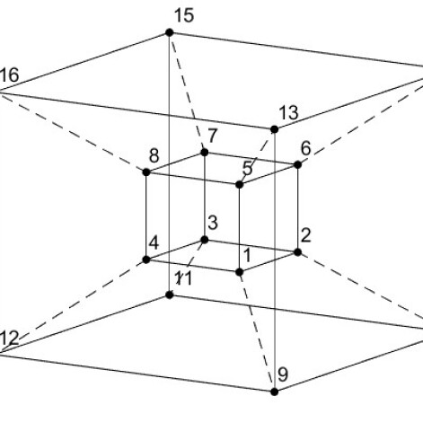
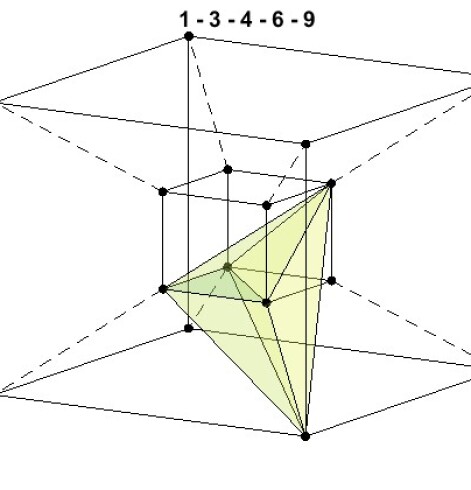
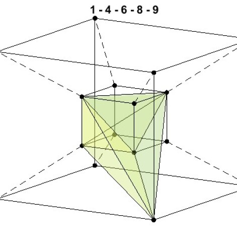
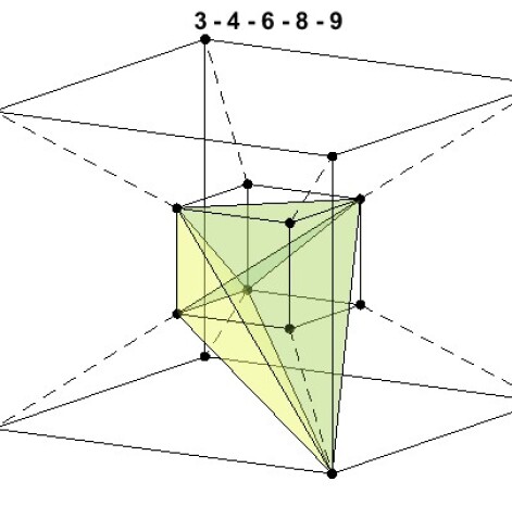
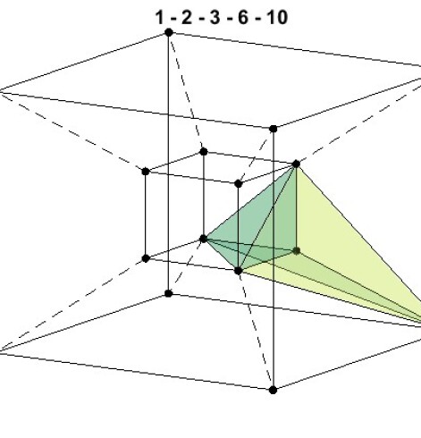
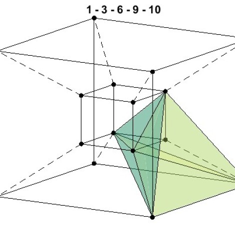
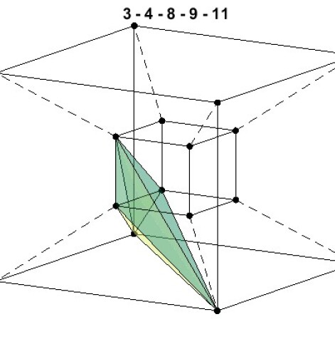
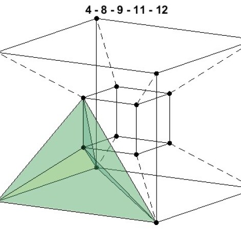
Figure 1: Illustration of the bounding tesseract sectioned into pentatopes (1-7), for the subdivision strategy with $N_{b}=23$.

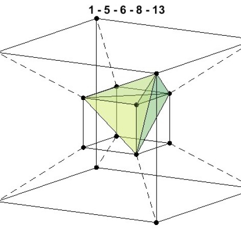
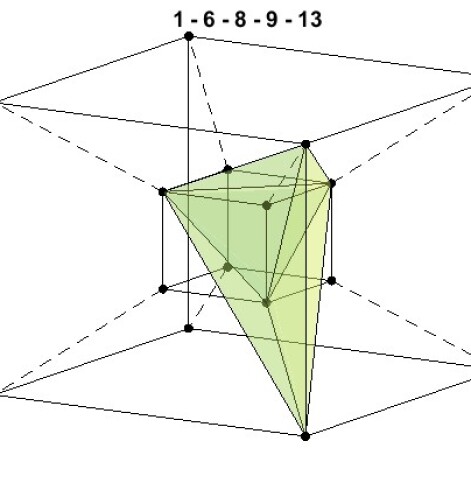
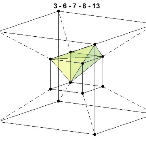
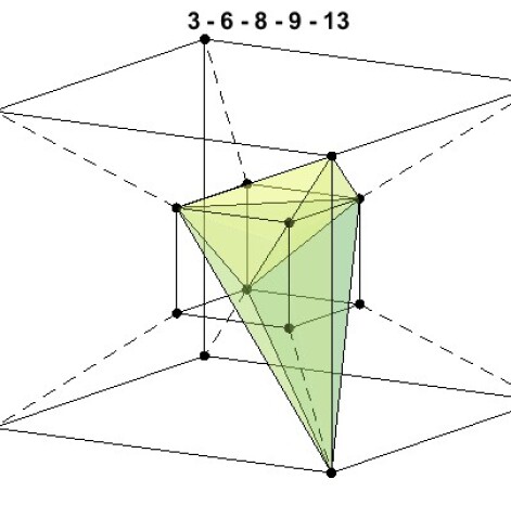
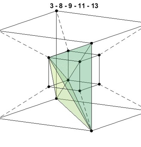
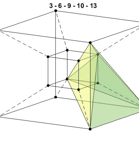
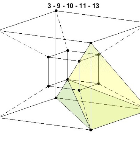
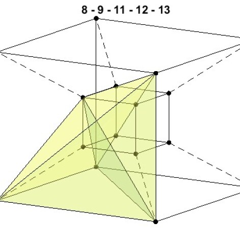
Figure 2: Illustration of the bounding tesseract sectioned into pentatopes (8-15), for the subdivision strategy with $N_{b}=23$.

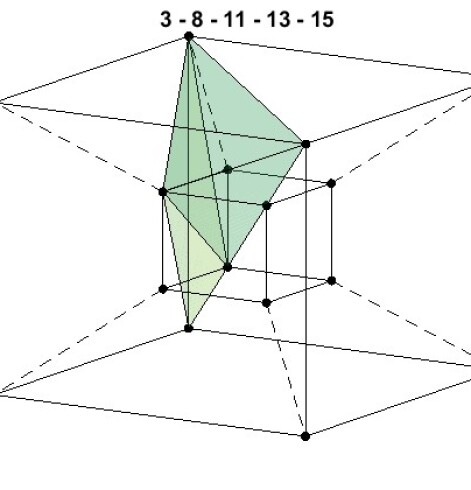
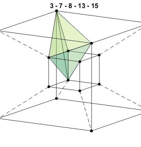
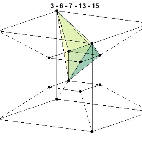
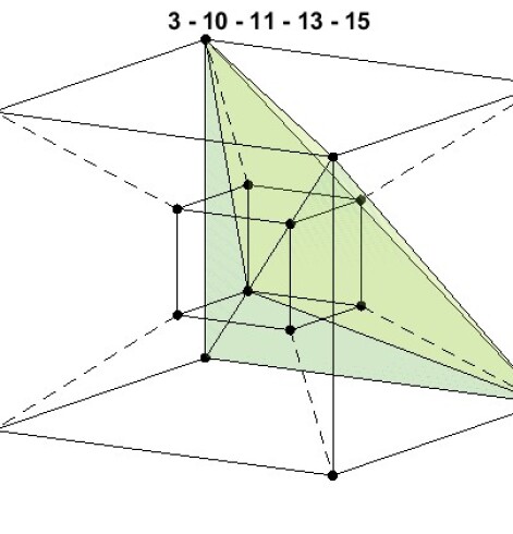
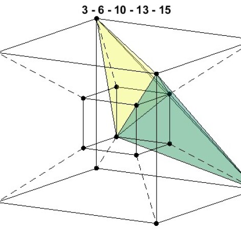
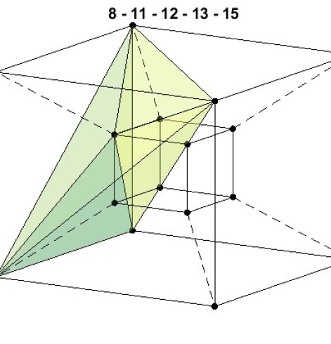
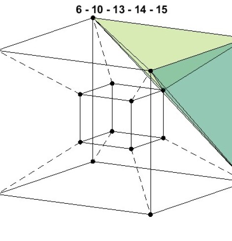
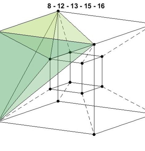
Figure 3: Illustration of the bounding tesseract sectioned into pentatopes (16-23), for the subdivision strategy with $N_{b}=23$.

3.2 Base Element Search

We begin by finding a pentatope element, referred to as the base element, that contains the point $p$ to be inserted. There are two prominent methods for identifying the base element: i) Lo’s method [9] which relies on calculating a series of volumes involving $p$, and ii) Si’s method [3] which relies on calculating a series of orientations of $p$ relative to the tetrahedron’s faces. Although both methods are effective, we proceeded with Si’s orientation-based method because it may be supplemented with the 4D orientation predicate for further accuracy. Scaled up to 4D, the method starts by identifying the tetrahedral facets associated with a given pentatope, then forming five temporary pentatopes from each facet combined with $p$. If each of the five temporary pentatopes n has an orientation $\theta$ greater than or equal to zero, or each has an orientation $\theta$ less than or equal to zero, $p$ is located inside of the pentatope, making it the base element. Pseudocode for this condition is shown below.

if $\theta_{n}\geq$ 0 $\forall n$ then

 inside = true

else if $\theta_{n}\leq$ 0 $\forall n$ then

 inside = true

else

 inside = false

end if

If $p$ does not lie within the pentatope, the orientations for each of the temporary pentatopes help indicate the direction of the point relative to the current pentatope. The facet associated with the temporary pentatope with the smallest magnitude for its orientation out of the five is the facet closest to $p$. The neighboring pentatope sharing this tetrahedral facet is then selected as the next candidate for the base element, and the process is repeated until the base element is found, forming a path from the first pentatope tested. A simple 2D illustration of a search path to the base element is shown in Figure 4.

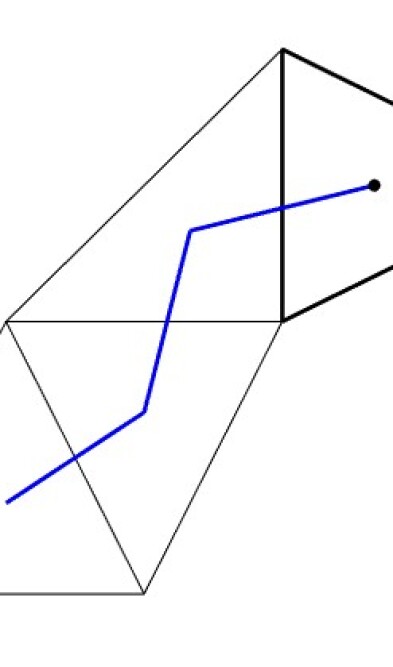
Figure 4: 2D illustration of finding the base element.

One of the most common problems encountered during a search for the base element is a search path forming a continuous closed loop within a specific set of elements. This occurs naturally due to limitations of the methodology. Fortunately, this problem can be easily remedied by keeping track of elements that have already been searched and not allowing the algorithm to return to them. Doing this will force a non-repeating path to be formed; although, the path may not be as direct as one would draw manually. If for some reason the number of iterations in searching for the base element exceeds the number of elements currently in the mesh without finding the base element, it may be useful to switch to an alternate strategy by performing a global search through all of the elements. Resorting to a global search in cases where an unresolved search path is formed should be a rare occurrence, and its frequency may indicate issues with the implementation of the element search, for example, issues with the accuracy of the predicates.

Another common issue worth mentioning is the appearance of ghost points, meaning points to be inserted that are found to not be contained in any existing pentatope. For an arrangement of coplanar (hypercoplanar) points, points to be inserted will often lie on a tetrahedral facet shared by two pentatopes. Due to limitations in machine precision, points lying directly on tetrahedral facets may be labeled as not belonging to either pentatope sharing that tetrahedral facet. This issue also extends to points located on other common features such as shared triangular faces and edges. One can avoid this issue by carefully setting tolerances associated with the resulting values of the orientation predicates for the base element test instead of comparing directly to zero.

3.3 Cavity Operator

Once the base pentatope has been identified, a cavity is formed by identifying the neighboring pentatopes with circumhyperspheres that contain point $p$, in accordance with the standard Delaunay criterion. The facet neighbors of the base pentatope make up an initial neighbor front. Each pentatope in the neighbor front is tested to see if its circumhypersphere contains point $p$. The check for the presence of a point within a circumhypersphere is called an in-hypersphere check. If the point is within a pentatope’s circumhypersphere, it is added to the cavity and its neighbors are added to the neighbor front if they do not yet belong to the cavity, and are not already a part of the neighbor front. Once the neighbor front is empty, meaning none of the pentatopes at the outside boundary of the cavity contain point $p$ in their respective circumhyperspheres, the process ends, and the cavity is considered complete.

Next, it is necessary to evaluate the validity of the cavity. For our purposes, a cavity is considered valid if point $p$ is visible to all the cavity’s bounding tetrahedral facets. Facet visibility is determined by calculating the dot product (denoted by $V$) between two vectors – the normal, inward facing vector of the facet ($\vv{N}$) and the vector formed between the facet’s centroid $c$ and point $p$ ($\vv{CP}$),

$$V=\vv{N}\cdot\vv{CP}.$$

In order to control visibility, one must set a lower limit on the value of $V$. The limit set on the value $V$ is heavily dependent on the user and their desired application, as it essentially represents the minimum quality for elements that the user is willing to accept. $V=0$ means that when a facet is reconnected to $p$, the pentatope formed will have no hypervolume, and positive values close to zero will form slivers. Although the user may decide, we will note that four dimensions introduces greater complexity, and the point insertion algorithm begins to lose stability the further the tolerance is set above zero. For our purposes in creating an initial hypervolume mesh from a given hypersurface mesh, the limit of $V$ is set to double precision $(10^{-16})$, and all slivers with hypervolumes within double precision are accepted. The accuracy of $V$ is very important, which is why it is recommended that this value is calculated using quadruple precision.

If $V$ is negative or less than a tolerance specified by the user, the facet is considered not visible to point $p$. The pentatope associated with this facet is then removed from the cavity. This process continues until all the cavity’s bounding facets have visibility to point $p$. There is no scenario where all the pentatopes associated with the cavity are removed. If this occurs, it is an indication that the proposed algorithm has not been properly implemented, and one should check for consistent element orientation and proper removal of pentatopes associated with invisible facets.

3.4 Reconnection and Review

After an initial cavity has been identified and all its bounding tetrahedral facets have been deemed visible relative to point $p$, the pentatopes belonging to the cavity are removed from the mesh and replaced with pentatopes formed by connecting the bounding tetrahedral facets of the cavity to the inserted point. To ensure consistent orientation, each new pentatope’s local indexing is carefully specified to have a positive orientation. The entire point insertion process continues until all points from the hypersurface mesh have been inserted into the bounding tesseract.

A complete summary of the point insertion process appears below:

1. Locate the base pentatope.

2. Evaluate the neighbor front until an initial cavity is defined.

3. Remove pentatopes from the cavity until all the bounding tetrahedral facets are visible to the point to be inserted.

4. Remove pentatopes associated with the cavity. Then connect the cavity’s tetrahedral facets to the newly inserted point to form new pentatopes.

5. Ensure positive orientations of all new pentatopes.

A common error one may encounter when first attempting to implement this process is to find that points are still missing from the tessellation after the insertion algorithm has supposedly added all of the points. This stems from a lack of accuracy when identifying pentatopes belonging to each cavity – i.e. pentatopes that contain the point $p$ within their respective circumhyperspheres (see Section 3.3). If one is already using a 4D geometric predicate for this process, it my be insufficiently accurate, and changes may need to be implemented in accordance with Section 4.

4 Geometric Predicates

The two tests that appear throughout the point insertion algorithm, 4D orientation and in-hypersphere, hinge on the precision of Shewchuk’s floating-point arithmetic and predicates. Shewchuk pioneered the geometric predicates in 2D and 3D [43], and our use of them in 4D is simply an extension of his work. Shewchuk’s floating point arithmetic is a list of simple arithmetic operations that also keep track of the round-off error associated with each operation. For example, adding two variables, $a$ and $b$, results in a new variable $x$ and its associated round-off error $x_{\mathrm{roundoff}}$ as shown below:

$$x=a+b$$

$$b_{\mathrm{virtual}}=x-a$$

$$a_{\mathrm{virtual}}=x-b_{\mathrm{virtual}}$$

$$b_{\mathrm{roundoff}}=b-b_{\mathrm{virtual}}$$

$$a_{\mathrm{roundoff}}=a-a_{\mathrm{virtual}}$$

$$x_{\mathrm{roundoff}}=a_{\mathrm{roundoff}}+b_{\mathrm{roundoff}}.$$

The large matrix determinants required for calculating the 4D orientation and in-hypersphere predicates can be reduced to a combination of simple arithmetic operations. In turn, one may generate a more accurate result by accounting for round-off error throughout these simple operations, and adjusting the precision as necessary. The breakdown of these determinants are detailed in the following subsections and B.

4.1 4D Orientation Predicate

We start with the orientation predicate for a pentatope

$$Orientation=\begin{vmatrix}a_{x}&a_{y}&a_{z}&a_{t}&1\\ b_{x}&b_{y}&b_{z}&b_{t}&1\\ c_{x}&c_{y}&c_{z}&c_{t}&1\\ d_{x}&d_{y}&d_{z}&d_{t}&1\\ e_{x}&e_{y}&e_{z}&e_{t}&1\end{vmatrix},$$

and find that

$$Orientation=abcd+bcde+cdea+deab+eabc,$$

where $abcd$, $bcde$, $cdea$, $deab$, and $eabc$ are $4\times 4$ determinants. These determinants can be written explicitly as follows

$$abcd =\begin{vmatrix}a_{x}&a_{y}&a_{z}&a_{t}\\ b_{x}&b_{y}&b_{z}&b_{t}\\ c_{x}&c_{y}&c_{z}&c_{t}\\ d_{x}&d_{y}&d_{z}&d_{t}\end{vmatrix}=-a_{t}(bcd)+b_{t}(cda)-c_{t}(abd)+d_{t}(abc),$$

$$bcde =\begin{vmatrix}b_{x}&b_{y}&b_{z}&b_{t}\\ c_{x}&c_{y}&c_{z}&c_{t}\\ d_{x}&d_{y}&d_{z}&d_{t}\\ e_{x}&e_{y}&e_{z}&e_{t}\end{vmatrix}=-b_{t}(cde)+c_{t}(deb)-d_{t}(bce)+e_{t}(bcd),$$

$$cdea =\begin{vmatrix}c_{x}&c_{y}&c_{z}&c_{t}\\ d_{x}&d_{y}&d_{z}&d_{t}\\ e_{x}&e_{y}&e_{z}&e_{t}\\ a_{x}&a_{y}&a_{z}&a_{t}\end{vmatrix}=-c_{t}(dea)+d_{t}(eac)-e_{t}(cda)+a_{t}(cde),$$

$$deab =\begin{vmatrix}d_{x}&d_{y}&d_{z}&d_{t}\\ e_{x}&e_{y}&e_{z}&e_{t}\\ a_{x}&a_{y}&a_{z}&a_{t}\\ b_{x}&b_{y}&b_{z}&b_{t}\end{vmatrix}=-d_{t}(eab)+e_{t}(abd)-a_{t}(deb)+b_{t}(dea),$$

$$eabc =\begin{vmatrix}e_{x}&e_{y}&e_{z}&e_{t}\\ a_{x}&a_{y}&a_{z}&a_{t}\\ b_{x}&b_{y}&b_{z}&b_{t}\\ c_{x}&c_{y}&c_{z}&c_{t}\end{vmatrix}=-e_{t}(abc)+a_{t}(bce)-b_{t}(eac)+c_{t}(eab).$$

Here, the terms $abc$, $bce$, etc. are $3\times 3$ determinants. The explicit formulas for these determinants appear in B.1, where they are further reduced to combinations of $2\times 2$ determinants that may then be written as a series of arithmetic operations from Shewchuk’s method for floating-point arithmetic.

4.2 4D In-Hypersphere Predicate

The in-hypersphere predicate for a pentatope takes the following form

$$InHypersphere=\begin{vmatrix}a_{x}&a_{y}&a_{z}&a_{t}&a_{x}^{2}+a_{y}^{2}+a_{z}^{2}+a_{t}^{2}&1\\ b_{x}&b_{y}&b_{z}&b_{t}&b_{x}^{2}+b_{y}^{2}+b_{z}^{2}+b_{t}^{2}&1\\ c_{x}&c_{y}&c_{z}&c_{t}&c_{x}^{2}+c_{y}^{2}+c_{z}^{2}+c_{t}^{2}&1\\ d_{x}&d_{y}&d_{z}&d_{t}&d_{x}^{2}+d_{y}^{2}+d_{z}^{2}+d_{t}^{2}&1\\ e_{x}&e_{y}&e_{z}&e_{t}&e_{x}^{2}+e_{y}^{2}+e_{z}^{2}+e_{t}^{2}&1\\ f_{x}&f_{y}&f_{z}&f_{t}&f_{x}^{2}+f_{y}^{2}+f_{z}^{2}+f_{t}^{2}&1\end{vmatrix},$$

and equivalently

$$InHypersphere=-bcdef+cdefa-defab+efabc-fabcd+abcde,$$

where $bcdef$, $cdefa$, $defab$, $efabc$, $fabcd$, and $abcde$ are $5\times 5$ determinants. It can also be shown that

$$InHypersphere=a_{det}-b_{det}+c_{det}-d_{det}+e_{det}-f_{det},$$

where

$$a_{det} =(a_{x}^{2}+a_{y}^{2}+a_{z}^{2}+a_{t}^{2})(cdef+defb+bcef+bcde-bcdf),$$

$$b_{det} =(b_{x}^{2}+b_{y}^{2}+b_{z}^{2}+b_{t}^{2})(cdef+defa+efac+cdfa-cdea),$$

$$c_{det} =(c_{x}^{2}+c_{y}^{2}+c_{z}^{2}+c_{t}^{2})(defa+efab+fabd+abde-defb),$$

$$d_{det} =(d_{x}^{2}+d_{y}^{2}+d_{z}^{2}+d_{t}^{2})(bcef+efab+fabc+abce-efac),$$

$$e_{det} =(e_{x}^{2}+e_{y}^{2}+e_{z}^{2}+e_{t}^{2})(bcdf+cdfa+fabc+abcd-fabd),$$

$$f_{det} =(f_{x}^{2}+f_{y}^{2}+f_{z}^{2}+f_{t}^{2})(bcde+cdea+abde+abcd-abce).$$

Here, the terms $cdef$, $defb$, etc. are $4\times 4$ determinants. The $5\times 5$ and $4\times 4$ determinants described above are explicitly tabulated in B.2, where they are further reduced to combinations of $2\times 2$ determinants.

4.3 Data Structures and Predicate Precision

There is a direct link between our choice of data structure and the necessary level of precision for computing predicates. Generally speaking, the more connectivity information stored by a data structure, the less predicate calculations will be necessary. Data structures with very little connectivity information essentially must calculate the local connectivity between facets, vertices, etc. on-the-fly using predicates. This puts a lot of pressure on the accuracy of the predicates, as one mistake can result in a complete failure of the point-insertion process. Based on this observation, it would seem that data structures with more connectivity information would be preferred. However, storing more connectivity information also results in data structures which are very bulky and expensive to update, or navigate through. Thus, there is a direct tradeoff between the efficiency of a data structure, and the efficiency of the geometric predicate calculations.

Thus far, we have experimented with two, somewhat naive strategies for storing data. The first strategy involves a region-to-region data structure, which keeps a global list of pentatopes within the mesh, and another list of the pentatope-to-facet connectivity. These two structures are updated after each point is inserted. Although this strategy allows for immediate access to the facet neighbors of any element, it is computationally expensive to update, and the update process grows exponentially slower as the number of elements in the mesh increases.

The second strategy involves a vertex-to-region data structure, where each point in the mesh has a corresponding list of pentatopes that are connected to it. Here, a global list of pentatopes is not created until the point insertion process is completed. Finding facet neighbors using this data structure is more complex than with the first strategy; however, because this structure is easy to update, it is significantly faster. Due to its speed, this has become our primary strategy for storing element data during point insertion. We note that other, more efficient strategies exist, such as the vertex-to-vertex data structure of [44], and the half-facet structure of [45]. However, in our limited experience, the vertex-to-vertex data structure requires extremely high precision predicates (in excess of quadruple precision) in order to maintain robustness. In addition, while the half-facet data structure is more promising, a detailed study of this approach is beyond the scope of the current paper.

For the sake of completeness, we compared the robustness of our two data storage strategies. Without the accuracy of Shewchuk’s approach (outlined above) the point insertion algorithm fails for both data structures within the first few iterations due to a lack of accuracy in calculating the geometric predicates. While using Shewchuk’s approach, we considered whether using quadruple precision variables in key calculations, such as the geometric predicates, element hypervolumes, and visibility of tetrahedral facets, would present an advantage over double precision variables. Both levels of precision produce valid meshes that include all of the inserted points, meaning none of the previously inserted points disappeared during the formation of a cavity in a subsequent iteration. Keeping in mind that our test cases have consisted solely of simple, convex geometries, it is likely that the implementation of quadruple precision variables will be necessary with more complex geometries.

Another use case for high precision variables becomes apparent when considering hypervolume creep. This phenomenon occurs when small geometric inaccuracies lead to the formation of invalid slivers during reconnection from the boundary facets of a cavity to a newly inserted point. Evidence of these slivers can be seen in the gradual increase in the difference between the original hypervolume of the bounding tesseract and the hypervolume of the mesh at various times during the point-insertion process. Quadruple precision variables help to prevent this and provide a more accurate indication of when it is occurring.

5 Quality Improvement

In this section, we introduce three explicit algebraic expressions for measuring the quality of pentatope elements. In addition, we introduce a wide-array of bistellar flip operations which can be used to improve element quality.

5.1 Pentatope Quality Metrics

Liu and Joe [46] developed a quality metric for any tetrahedron that ranges from zero to one, where zero is a flat, zero-volume tetrahedron, and one is a regular tetrahedron. Following the derivation of their metric, we arrive at a similar quality metric for pentatopes.

Theorem 5.1.

The quality of any pentatope $P(p_{0},p_{1},p_{2},p_{3},p_{4})$ can be determined by

$$\eta^{(1)}=\frac{5^{3/4}\sqrt{384v}}{\sum^{10}_{i=1}l^{2}_{i}},$$

where $v$ is the hypervolume, and $l_{i}$’s are the edge lengths of the pentatope. Here, ‘quality’ is defined as the degree of similarity between an arbitrary pentatope and a regular pentatope with the same hypervolume.

Proof.

Consider a regular pentatope $P_{r}(r_{0},r_{1},r_{2},r_{3},r_{4})$ with edge length $a$, and the same hypervolume as an arbitrary pentatope $P(p_{0},p_{1},p_{2},p_{3},p_{4})$. The coordinates of the regular pentatope are defined as $r_{0}=(-a\sqrt{3}/2,0,0,0)$, $r_{1}=(0,-a/2,0,0)$, $r_{2}=(0,a/2,0,0)$, $r_{3}=(-a\sqrt{3}/6,0,a\sqrt{6}/3,0)$, and $r_{4}=(-a\sqrt{3}/6,0,a\sqrt{6}/12,a\sqrt{10}/4)$. Let $R=[(r_{1}-r_{0}),(r_{2}-r_{0}),(r_{3}-r_{0}),(r_{4}-r_{0})]$ and $T=[(p_{1}-p_{0}),(p_{2}-p_{0}),(p_{3}-p_{0}),(p_{4}-p_{0})]$. Then

$$R=a\begin{bmatrix}\sqrt{3}/2&\sqrt{3}/2&\sqrt{3}/3&\sqrt{3}/3\\ -1/2&1/2&0&0\\ 0&0&\sqrt{6}/3&\sqrt{6}/12\\ 0&0&0&\sqrt{10}/4\end{bmatrix},\qquad R^{-1}=\frac{1}{a}\begin{bmatrix}\frac{\sqrt{3}}{3}&-1&-\frac{\sqrt{6}}{6}&-\frac{\sqrt{10}}{10}\\ \frac{\sqrt{3}}{3}&1&-\frac{\sqrt{6}}{6}&-\frac{\sqrt{10}}{10}\\ 0&0&\frac{\sqrt{6}}{2}&-\frac{\sqrt{10}}{10}\\ 0&0&0&\frac{2\sqrt{10}}{5}\end{bmatrix},$$

and

$$T^{T}T=\begin{bmatrix}d_{01}&(d_{01}+d_{02}-d_{12})/{2}&(d_{01}+d_{03}-d_{13})/{2}&(d_{01}+d_{04}-d_{14})/{2}\\ (d_{01}+d_{02}-d_{12})/{2}&d_{02}&(d_{02}+d_{03}-d_{23})/{2}&(d_{02}+d_{04}-d_{24})/{2}\\ (d_{01}+d_{03}-d_{13})/{2}&(d_{02}+d_{03}-d_{23})/{2}&d_{03}&(d_{03}+d_{04}-d_{34})/{2}\\ (d_{01}+d_{04}-d_{14})/{2}&(d_{02}+d_{04}-d_{24})/{2}&(d_{03}+d_{04}-d_{34})/{2}&d_{04}\end{bmatrix}.$$

Here, $a=(96v/\sqrt{5})^{1/4}$ and $d_{ij}=(t_{j}-t_{i})^{T}(t_{j}-t_{i})$, $0\leq i<j\leq 4$. The hypervolume $v$ is defined as

$$v =\frac{\sqrt{d+1}}{2^{d/2}d!}a^{d}=\frac{\sqrt{4+1}}{2^{4/2}4!}a^{4}=\frac{\sqrt{5}}{96}a^{4}.$$

Next, we define

$$A(R,T)\equiv(R^{-1})^{T}T^{T}TR^{-1}=\frac{1}{a^{2}}\begin{bmatrix}\alpha&\#&\#&\#\\ \#&\beta&\#&\#\\ \#&\#&\gamma&\#\\ \#&\#&\#&\delta\end{bmatrix},$$

where $\alpha=(2d_{01}+2d_{02}-d_{12})/3$, $\beta=d_{12}$, $\gamma=(3d_{03}+3d_{23}+3d_{13}-d_{01}-d_{02}-d_{12})/6$, and $\delta=(4d_{04}+4d_{14}+4d_{24}+4d_{34}-d_{01}-d_{02}-d_{03}-d_{12}-d_{13}-d_{23})/10$. In addition, irrelevant values are indicated by the # sign.

The quality metric $\eta^{(1)}$ can be defined as the ratio of the geometric and arithmetic means for the inscribed 4-ellipsoid in the pentatope. As a result, $\eta^{(1)}$ can be written as follows

$$\eta^{(1)}\equiv\frac{4\sqrt[4]{\lambda_{1}\lambda_{2}\lambda_{3}\lambda_{4}}}{\lambda_{1}+\lambda_{2}+\lambda_{3}+\lambda_{4}},$$ (5.1)

where $\lambda_{1}$, $\lambda_{2}$, $\lambda_{3}$, and $\lambda_{4}$ are the eigenvalues of $A(R,T)$. Next, we have that

$$\lambda_{1}+\lambda_{2}+\lambda_{3}+\lambda_{4} =\mathrm{trace}(A(R,T))$$

$$=\frac{2}{5a^{2}}(d_{01}+d_{02}+d_{03}+d_{04}+d_{12}+d_{13}+d_{14}+d_{23}+d_{24}+d_{34})$$

$$=\frac{2}{5a^{2}}\sum^{10}_{i=1}l^{2}_{i}.$$ (5.2)

Because $P_{r}$ and $P$ have the same hypervolume,

$$\lambda_{1}\lambda_{2}\lambda_{3}\lambda_{4}=\mathrm{det}(A(R,T))=1.$$ (5.3)

By substituting Eqs. (5.2) and (5.3) into Eq. (5.1), the desired quality metric for a pentatope is obtained

$$\eta^{(1)} =\frac{4\sqrt[4]{\mathrm{det}(A(R,T))}}{\mathrm{trace}(A(R,T))}=\frac{4}{\frac{2}{5a^{2}}\sum^{10}_{i=1}l^{2}_{i}}=\frac{10\Bigg{(}\frac{96}{\sqrt{5}}v\Bigg{)}^{1/2}}{\sum^{10}_{i=1}l^{2}_{i}}=\frac{5^{3/4}\sqrt{384v}}{\sum^{10}_{i=1}l^{2}_{i}}.$$

∎

Corollary 5.2.

The quality of any pentatope $P(p_{0},p_{1},p_{2},p_{3},p_{4})$ can be determined by

$$\eta^{(2)}=\frac{6\sum^{10}_{i=1}l^{2}_{i}}{\sqrt{\Theta\left(\left\{l_{i}^{2}\right\}_{i=1}^{10}\right)}},$$

where $l_{i}$ are the edge lengths of the pentatope, and

$$\Theta\left(\left\{l_{i}^{2}\right\}_{i=1}^{10}\right) \equiv 600(l_{1}^{2}-l_{2}^{2})^{2}+900l_{5}^{4}+100(-2(l_{1}^{2}+l_{2}^{2})+l_{5}^{2})^{2}$$

$$+75(l_{1}^{2}-l_{2}^{2}-3l_{6}^{2}+3l_{8}^{2})^{2}+25(l_{1}^{2}+l_{2}^{2}-3l_{3}^{2}+l_{5}^{2}-3(l_{6}^{2}+l_{8}^{2}))^{2}$$

$$+25(l_{1}^{2}+l_{2}^{2}-6l_{3}^{2}-2l_{5}^{2}+3(l_{6}^{2}+l_{8}^{2}))^{2}$$

$$+45(l_{1}^{2}-l_{2}^{2}+l_{6}^{2}-4l_{7}^{2}-l_{8}^{2}+4l_{9}^{2})^{2}$$

$$+15(l_{1}^{2}+l_{2}^{2}+2l_{3}^{2}-8l_{4}^{2}-2l_{5}^{2}-l_{6}^{2}+4l_{7}^{2}-l_{8}^{2}+4l_{9}^{2})^{2}$$

$$+30(-l_{1}^{2}-l_{2}^{2}+l_{3}^{2}+2l_{4}^{2}-l_{5}^{2}+l_{6}^{2}+2l_{7}^{2}+l_{8}^{2}+2l_{9}^{2}-6l_{10}^{2})^{2}$$

$$+9(l_{1}^{2}+l_{2}^{2}+l_{3}^{2}-4l_{4}^{2}+l_{5}^{2}+l_{6}^{2}-4l_{7}^{2}+l_{8}^{2}-4(l_{9}^{2}+l_{10}^{2}))^{2}.$$

Proof.

In the previous theorem, a quality metric was defined based on the ratio of the geometric and arithmetic means of the pentatope’s inscribed 4-ellipsoid. It turns out, we can also define a metric based on the ratio of the arithmetic mean and the root-mean-square (RMS) as follows

$$\eta^{(2)}\equiv\frac{\lambda_{1}+\lambda_{2}+\lambda_{3}+\lambda_{4}}{2\sqrt{\lambda_{1}^{2}+\lambda_{2}^{2}+\lambda_{3}^{2}+\lambda_{4}^{2}}}.$$ (5.4)

The denominator of this expression is twice the Frobenius norm of $A(R,T)$

$$\sqrt{\lambda_{1}^{2}+\lambda_{2}^{2}+\lambda_{3}^{2}+\lambda_{4}^{2}} =\sqrt{\mathrm{trace}(A(R,T)A(R,T)^{T})}=\left\|A(R,T)\right\|_{F}$$

$$=\frac{1}{30a^{2}}\Big{[}600(d_{01}-d_{02})^{2}+900d_{12}^{2}+100(-2(d_{01}+d_{02})+d_{12})^{2}$$

$$+75(d_{01}-d_{02}-3d_{13}+3d_{23})^{2}+25(d_{01}+d_{02}-3d_{03}+d_{12}-3(d_{13}+d_{23}))^{2}$$

$$+25(d_{01}+d_{02}-6d_{03}-2d_{12}+3(d_{13}+d_{23}))^{2}$$

$$+45(d_{01}-d_{02}+d_{13}-4d_{14}-d_{23}+4d_{24})^{2}$$

$$+15(d_{01}+d_{02}+2d_{03}-8d_{04}-2d_{12}-d_{13}+4d_{14}-d_{23}+4d_{24})^{2}$$

$$+30(-d_{01}-d_{02}+d_{03}+2d_{04}-d_{12}+d_{13}+2d_{14}+d_{23}+2d_{24}-6d_{34})^{2}$$

$$+9(d_{01}+d_{02}+d_{03}-4d_{04}+d_{12}+d_{13}-4d_{14}+d_{23}-4(d_{24}+d_{34}))^{2}\Big{]}^{1/2}$$

$$=\frac{1}{30a^{2}}\sqrt{\Theta(d_{01},d_{02},d_{03},d_{04},d_{12},d_{13},d_{14},d_{23},d_{24},d_{34})}$$

$$=\frac{1}{30a^{2}}\sqrt{\Theta\left(l_{1}^{2},l_{2}^{2},l_{3}^{2},l_{4}^{2},l_{5}^{2},l_{6}^{2},l_{7}^{2},l_{8}^{2},l_{9}^{2},l_{10}^{2}\right)}=\frac{1}{30a^{2}}\sqrt{\Theta\left(\left\{l_{i}^{2}\right\}_{i=1}^{10}\right)}.$$ (5.5)

Next, if we substitute Eqs. (5.2) and (5.5) into Eq. (5.4) we obtain the desired result

$$\eta^{(2)}=\frac{\mathrm{trace}(A(R,T))}{2\sqrt{\mathrm{trace}(A(R,T)A(R,T)^{T})}}=\frac{\frac{2}{5a^{2}}\sum^{10}_{i=1}l^{2}_{i}}{\frac{2}{30a^{2}}\sqrt{\Theta\left(\left\{l_{i}^{2}\right\}_{i=1}^{10}\right)}}=\frac{6\sum^{10}_{i=1}l^{2}_{i}}{\sqrt{\Theta\left(\left\{l_{i}^{2}\right\}_{i=1}^{10}\right)}}.$$

∎

Corollary 5.3.

The quality of any pentatope $P(p_{0},p_{1},p_{2},p_{3},p_{4})$ can be determined by

$$\eta^{(3)}=6\cdot 5^{3/4}\sqrt{\frac{384v}{\Theta\left(\left\{l_{i}^{2}\right\}_{i=1}^{10}\right)}},$$

where $v$ is the hypervolume, and $l_{i}$’s are the edge lengths of the pentatope.

Proof.

The quality metric above is simply the ratio of the geometric mean and the RMS, for the inscribed 4-ellipsoid. We can obtain this quality metric immediately by multiplying the quality metrics of Theorem 5.1 and Corollary 5.2 together. ∎

Remark 5.4.

Suppose that the eigenvalues of the inscribed 4-ellipsoid are non-negative, i.e. $\lambda_{1}\geq 0$, $\lambda_{2}\geq 0$, $\lambda_{3}\geq 0$, and $\lambda_{4}\geq 0$. Under these circumstances, it is well known that the following relationship holds for the RMS, arithmetic mean (AM), and geometric mean (GM) of the eigenvalues

$$\mathrm{RMS}\geq\mathrm{AM}\geq\mathrm{GM}\geq 0.$$ (5.6)

Therefore, upon dividing Eq. (5.6) by the RMS, we conclude that

$$1\geq\eta^{(2)}\geq\eta^{(3)}\geq 0.$$

In addition, upon dividing Eq. (5.6) by the AM, we conclude that

$$1\geq\eta^{(1)}\geq 0.$$

Therefore, each quality measure is guaranteed to lie on the interval $[0,1]$. In addition, the third quality measure is generally, more conservative than the second.

5.2 Bistellar Flips

Bistellar flips have been used successfully in order to improve mesh quality, in accordance with the pioneering work of Shewchuk [47, 10]. Bistellar flips involve reconnecting/repartitioning groups of low quality elements to create alternative groups of higher quality elements, while simultaneously maintaining the original external facets of the group. There exists $(d+1)$ possible flipping operations in each dimension, which are associated with the transformations of $k$ elements into $(d+2)-k$ elements, where d is the number of dimensions and $k$ is the number of initial elements. In 4D, the five basic flipping operations are: $(1\rightarrow 5)$, $(2\rightarrow 4)$, $(3\rightarrow 3)$, $(4\rightarrow 2)$, and $(5\rightarrow 1)$. The number of vertices required for the starting and ending configurations can be determined by Eq. (5.7). The basic 4D bistellar flips and their corresponding connectivity transformations are shown in Figures 5-7. We note that some of the 3D representations of the 4D flips look identical before and after the transformation because the representation is essentially a shadow of a higher dimensional object, and is unable to capture all of its detail.

$$n_{vertex}=\begin{cases}d+1&\text{$if\quad k=1$}\\ d+2&\text{$if\quad k>1$}\end{cases}.$$ (5.7)

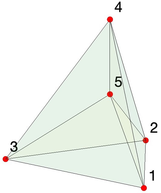
Stage 1 Stage 2 1 2 3 4 5 1 2 3 4 6 2 3 4 5 6 1 3 4 5 6 1 2 4 5 6 1 2 3 5 6

Figure 5: Flip ($1\rightarrow 5$) partitions one pentatope (left) into five (right) by inserting a point within the element and reconnecting. Reversing the process is also valid via flip ($5\rightarrow 1$). The table summarizes the connectivity transformation.

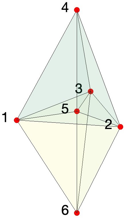
Stage 1 Stage 2 1 2 3 4 5 1 2 3 4 6 1 2 3 5 6 1 2 4 5 6 2 3 4 5 6 1 3 4 5 6

Figure 6: Flip ($2\rightarrow 4$) partitions two pentatopes into four through reconnection. The 3D representations of both configurations are identical. Reversing the process is also valid via flip ($4\rightarrow 2$). The table summarizes the connectivity transformation.

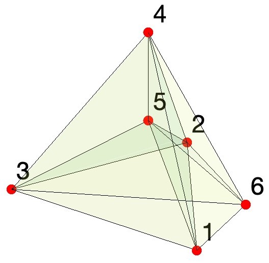
Stage 1 Stage 2 1 2 3 4 5 1 2 3 4 6 1 2 4 5 6 2 3 4 5 6 1 3 4 5 6 1 2 3 5 6

Figure 7: Flip ($3\rightarrow 3$) partitions three pentatopes into three alternative pentatopes through reconnection. 3D representations of both configurations are identical. Reversing the process is also valid. The table summarizes the connectivity transformation.

The basic 4D flips have already been identified in previous work; other authors refer to them as 4D Pachner moves [48]. Expanding on the basic set of 4D flips, we derive a new, more exhaustive set of possible flips by extending lower-dimensional flips into higher dimensions as shown in Table 4. These extended flips are formed by taking lower-dimensional subsimplices (facets, faces, or edges) of our pentatopes, performing lower-dimensional flips on these entities, then updating the connectivity. For example, suppose that a grouping of three pentatopes share a triangular face. This face can be split into three triangles by inserting a point and performing a $(1\rightarrow 3)$ flip in 2D. Thereafter, a reconnection operation can be performed in order to obtain nine pentatopes from the original three. This corresponds to an extended 4D flip, called a $(3\rightarrow 9)$ flip, which directly inherits from the lower-dimensional $(1\rightarrow 3)$ 2D flip. We have identified a total of 12 such extended flips, and the complete set is shown in Figures 8–19 along with their respective connectivity transformations. It is worth noting that some of the 4D extended flips have multiple versions. As an example, the 3D extended $(4\rightarrow 4)$ flip has three different $(8\rightarrow 8)$ configurations in 4D.

4D Extended Flips
$1D\Rightarrow 4D$	$2D\Rightarrow 4D$	$3D\Rightarrow 4D$
$(1\rightarrow 2)\Rightarrow(4\rightarrow 8)$	$(1\rightarrow 3)\Rightarrow(3\rightarrow 9)$	$(1\rightarrow 4)\Rightarrow(2\rightarrow 8)$
	$(2\rightarrow 2)\Rightarrow(6\rightarrow 6)$	$(2\rightarrow 3)\Rightarrow(4\rightarrow 6)$
	$(2\rightarrow 4)\Rightarrow(6\rightarrow 12)$a	$(4\rightarrow 4)\Rightarrow(8\rightarrow 8)^{*}$
		$(2\rightarrow 6)\Rightarrow(4\rightarrow 12)$
		$(3\rightarrow 6)\Rightarrow(6\rightarrow 12)$b
		$(4\rightarrow 8)\Rightarrow(8\rightarrow 16)$

Table 4: Lower dimensional flips extended to four dimensions. The * indicates that the $(8\rightarrow 8)$ flip has three different realizations.

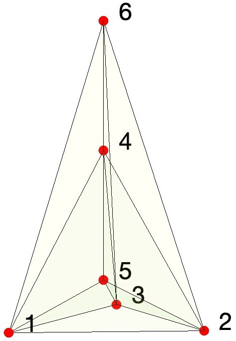
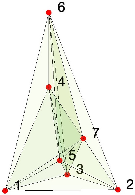
Stage 1 Stage 2 1 2 3 4 5 1 3 4 5 7 1 2 4 5 6 1 2 3 5 7 2 3 4 5 6 1 4 5 6 7 1 2 3 4 6 1 2 5 6 7 3 4 5 6 7 2 3 5 6 7 1 3 4 6 7 1 2 3 6 7

Figure 8: Flip ($4\rightarrow 8$) partitions four pentatopes (left) into eight (right) by inserting a point along the shared edge and reconnecting. Reversing the process is also valid via flip ($8\rightarrow 4$). The flip is a 4D extension of the 1D, ($1\rightarrow 2$) flip. The table summarizes the connectivity transformation.

Stage 1 Stage 2 1 2 3 4 5 1 2 3 4 7 1 2 4 5 6 1 3 4 5 7 2 3 4 5 6 1 2 3 5 7 1 4 5 6 7 1 2 5 6 7 1 2 4 6 7 3 4 5 6 7 2 3 5 6 7 2 3 4 6 7

Figure 9: Flip ($3\rightarrow 9$) partitions three pentatopes (left) into nine (right) by inserting a point within the shared triangle and reconnecting. Reversing the process is also valid via flip ($9\rightarrow 3$). The flip is a 4D extension of the 2D, ($1\rightarrow 3$) flip. The table summarizes the connectivity transformation.

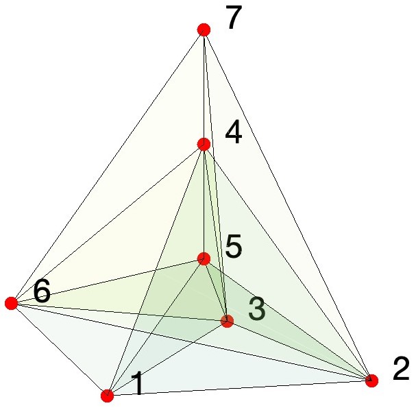
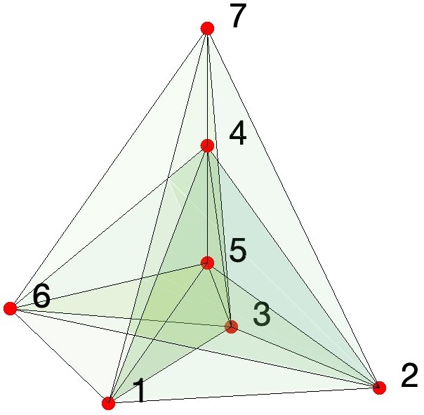
Stage 1 Stage 2 1 2 3 4 5 1 2 3 4 7 1 2 4 5 6 1 2 4 6 7 1 3 4 5 6 1 3 4 6 7 2 3 4 5 7 1 2 3 5 7 2 4 5 6 7 1 2 5 6 7 3 4 5 6 7 1 3 5 6 7

Figure 10: Flip ($6\rightarrow 6$) partitions six pentatopes (left) into six alternative pentatopes (right) through reconnection on the shared grouping of triangles. The flip is reversible. In addition, the flip is a 4D extension of the 2D, ($2\rightarrow 2$) flip. The table summarizes the connectivity transformation.

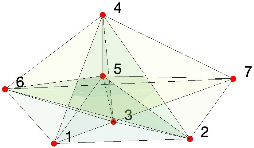
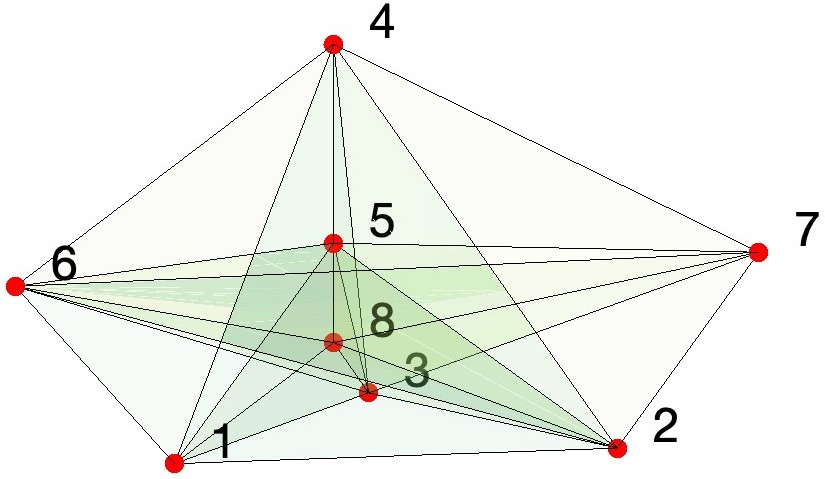
Stage 1 Stage 2 1 2 3 4 5 1 2 3 4 8 2 3 4 7 8 1 2 4 5 6 1 2 4 6 8 2 4 6 7 8 1 3 4 5 6 1 3 4 6 8 3 4 6 7 8 2 3 4 5 7 1 2 3 5 8 2 3 5 7 8 2 4 5 6 7 1 2 5 6 8 2 5 6 7 8 3 4 5 6 7 1 3 5 6 8 3 5 6 7 8

Figure 11: Flip ($6\rightarrow 12$)a partitions six pentatopes (left) into twelve (right) by inserting a point within the shared grouping of triangles and reconnecting. Reversing the process is also valid via flip ($12\rightarrow 6$)a. The flip is a 4D extension of the 2D, ($2\rightarrow 4$) flip. The table summarizes the connectivity transformation.

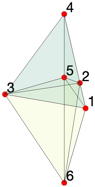
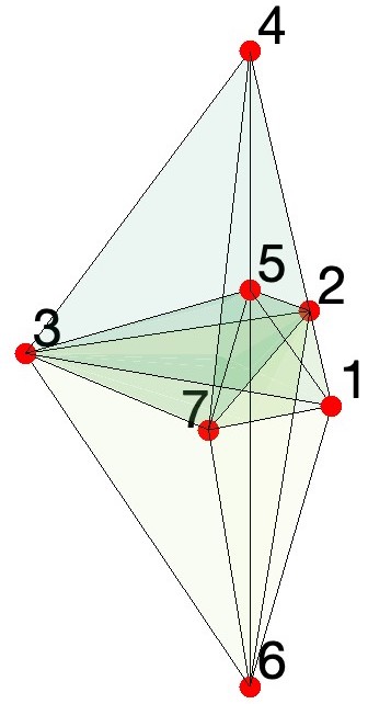
Stage 1 Stage 2 1 2 3 4 5 1 2 3 4 7 1 2 3 5 6 2 3 4 5 7 1 3 4 5 7 1 2 4 5 7 2 3 5 6 7 1 3 5 6 7 1 2 5 6 7 1 2 3 6 7

Figure 12: Flip ($2\rightarrow 8$) partitions two pentatopes (left) into eight (right) by inserting a point within the shared tetrahedron and reconnecting. Reversing the process is also valid via flip ($8\rightarrow 2$). The flip is a 4D extension of the 3D, ($1\rightarrow 4$) flip. The table summarizes the connectivity transformation.

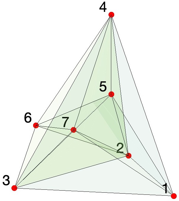
Stage 1 Stage 2 1 2 3 4 5 1 2 3 6 7 2 3 4 5 6 1 3 4 6 7 1 2 3 4 7 1 2 4 5 6 2 3 4 6 7 1 3 4 5 6 1 2 3 5 6 1 2 4 6 7

Figure 13: Flip ($4\rightarrow 6$) partitions four pentatopes into six through reconnection of a shared grouping of tetrahedra. The 3D representations of both configurations are identical. Reversing the process is also valid via flip ($6\rightarrow 4$). The flip is a 4D extension of the 3D, ($2\rightarrow 3$) flip. The table summarizes the connectivity transformation.

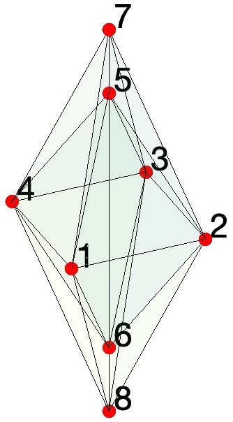
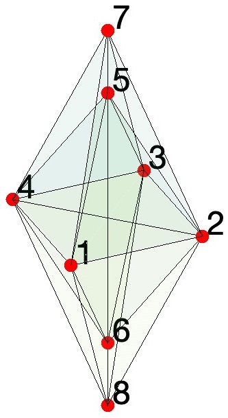
Stage 1 Stage 2 1 2 5 6 7 1 2 4 5 7 2 3 5 6 7 2 3 4 5 7 3 4 5 6 7 1 2 4 6 7 1 4 5 6 7 2 3 4 6 7 1 2 5 6 8 1 2 4 5 8 2 3 5 6 8 2 3 4 5 8 3 4 5 6 8 1 2 4 6 8 1 4 5 6 8 2 3 4 6 8

Figure 14: Flip ($8\rightarrow 8$) version 1, partitions eight pentatopes (left) into eight alternative pentatopes (right) through reconnection of a shared grouping of tetrahedra. The flip is reversible. In addition, the flip is a 4D extension of the 3D, ($4\rightarrow 4$) flip. The table summarizes the connectivity transformation.

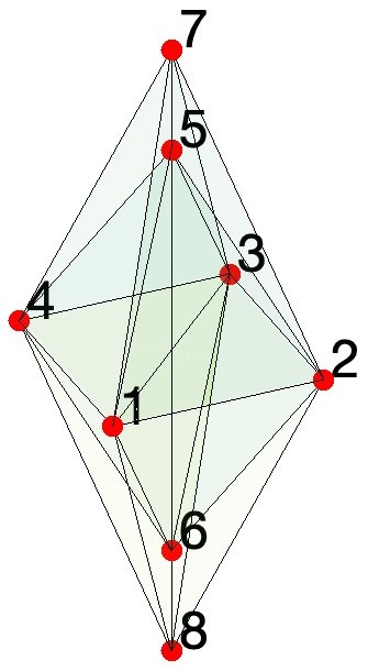
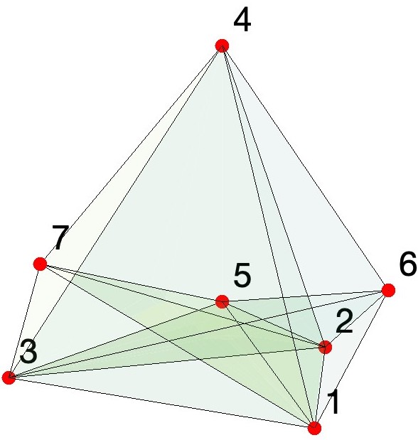
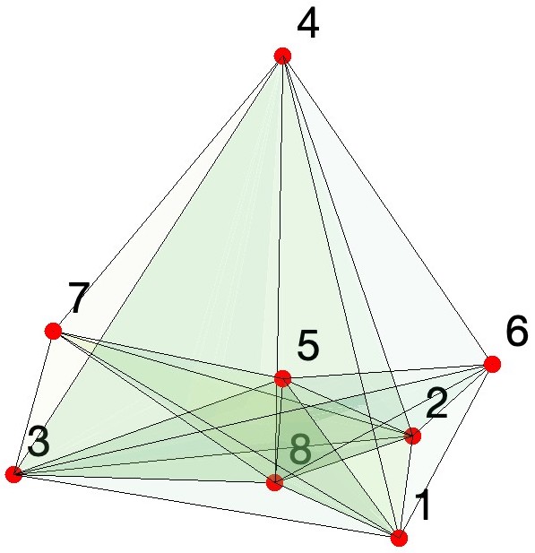
Stage 1 Stage 2 1 2 5 6 7 1 2 3 5 7 2 3 5 6 7 1 3 4 5 7 3 4 5 6 7 1 2 3 6 7 1 4 5 6 7 1 3 4 6 7 1 2 5 6 8 1 2 3 5 8 2 3 5 6 8 1 3 4 5 8 3 4 5 6 8 1 2 3 6 8 1 4 5 6 8 1 3 4 6 8

Figure 15: Flip ($8\rightarrow 8$) version 2, partitions eight pentatopes (left) into eight alternative pentatopes (right) through reconnection of a shared grouping of tetrahedra. The flip is reversible. In addition, the flip is a 4D extension of the 3D, ($4\rightarrow 4$) flip. The table summarizes the connectivity transformation.

Stage 1 Stage 2 1 2 4 5 7 1 2 3 5 7 2 3 4 5 7 1 3 4 5 7 1 2 4 6 7 1 2 3 6 7 2 3 4 6 7 1 3 4 6 7 1 2 4 5 8 1 2 3 5 8 2 3 4 5 8 1 3 4 5 8 1 2 4 6 8 1 2 3 6 8 2 3 4 6 8 1 3 4 6 8

Figure 16: Flip ($8\rightarrow 8$) version 3, partitions eight pentatopes (left) into eight alternative pentatopes (right) through reconnection of a shared grouping of tetrahedra. The flip is reversible. In addition, the flip is a 4D extension of the 3D, ($4\rightarrow 4$) flip. The table summarizes the connectivity transformation.

Stage 1 Stage 2 1 2 3 4 6 2 3 4 6 8 2 3 4 7 8 1 2 3 5 6 1 3 4 6 8 1 3 4 7 8 1 2 3 4 7 1 2 4 6 8 1 2 4 7 8 1 2 3 5 7 2 3 5 6 8 2 3 5 7 8 1 3 5 6 8 1 3 5 7 8 1 2 5 6 8 1 2 5 7 8

Figure 17: Flip ($4\rightarrow 12$) partitions four pentatopes (left) into twelve (right) by inserting a point within the shared triangle and reconnecting. Reversing the process is also valid via flip ($12\rightarrow 4$). The flip is a 4D extension of the 3D, ($2\rightarrow 6$) flip. The table summarizes the connectivity transformation.

Stage 1 Stage 2 1 2 4 5 6 1 2 5 6 8 1 2 5 7 8 2 3 4 5 6 1 2 4 6 8 1 2 4 7 8 1 3 4 5 6 2 3 5 6 8 2 3 5 7 8 1 2 4 5 7 2 3 4 6 8 2 3 4 7 8 2 3 4 5 7 1 3 5 6 8 1 3 5 7 8 1 3 4 5 7 1 3 4 6 8 1 3 4 7 8

Figure 18: Flip ($6\rightarrow 12$)b partitions six pentatopes (left) into twelve (right) by inserting a point within the shared grouping of tetrahedra and reconnecting. Reversing the process is also valid via flip ($12\rightarrow 6$)b. The flip is a 4D extension of the 3D, ($3\rightarrow 6$) flip. The table summarizes the connectivity transformation.

Stage 1 Stage 2 1 2 4 5 7 2 3 6 7 9 1 4 5 8 9 2 3 4 5 7 1 4 5 7 9 1 2 5 8 9 1 2 4 6 7 1 2 5 7 9 3 4 5 8 9 2 3 4 6 7 3 4 5 7 9 2 3 5 8 9 1 2 4 5 8 2 3 5 7 9 1 4 6 8 9 2 3 4 5 8 1 4 6 7 9 1 2 6 8 9 1 2 4 6 8 1 2 6 7 9 3 4 6 8 9 2 3 4 6 8 3 4 6 7 9 2 3 6 8 9

Figure 19: Flip ($8\rightarrow 16$) partitions eight pentatopes (left) into sixteen (right) by inserting a point on the shared edge and reconnecting. Reversing the process is also valid via flip ($16\rightarrow 8$). The flip is a 4D extension of the 3D, ($4\rightarrow 8$) flip. The table summarizes the connectivity transformation.

6 Numerical Examples

In this section, we assess the validity of our algorithms for point insertion and quality improvement. These algorithms were implemented as an extension of the JENRE${}^{\text{\textregistered}}$ Multiphysics Framework, which is United States government-owned software developed by the Naval Research Laboratory with other collaborating institutions. This software was used in earlier work for space-time finite element methods [37, 49].

6.1 Hypervolume Convergence Study

In this test, our objective was to demonstrate the validity of our Delaunay point-insertion algorithm by generating multiple hypervolume meshes, and assessing the volumetric error associated with each mesh. Towards this end, we began by constructing a simple hypercylinder geometry with a radius of $R=1$ and a length of $L=4$. The hypercylinder geometry consisted of a 3-sphere which was extruded in the temporal direction in order to generate a space-time cylinder, (as shown in Figure 20). We note that the hypercylinder is convenient to work with because it is convex. Based on the techniques of [37], we generated a family of tetrahedral hypersurface meshes which conformed to the hypercylinder geometry. The diameters of the tetrahedral elements in each mesh were controlled by the following parameters: $h_{\mathrm{sphere}}$, which prescribed the size of elements on the surface of each sphere; and $h_{\mathrm{time}}$, which prescribed the size of elements along the temporal axis of the hypercylinder. The family of meshes was generated by setting $h_{\mathrm{sphere}}=1$ and $h_{\mathrm{time}}=1$, and successively refining the meshes by reducing the parameters by factors of 1.5 or 2.0. The properties of each hypersurface mesh are summarized in Table 5.

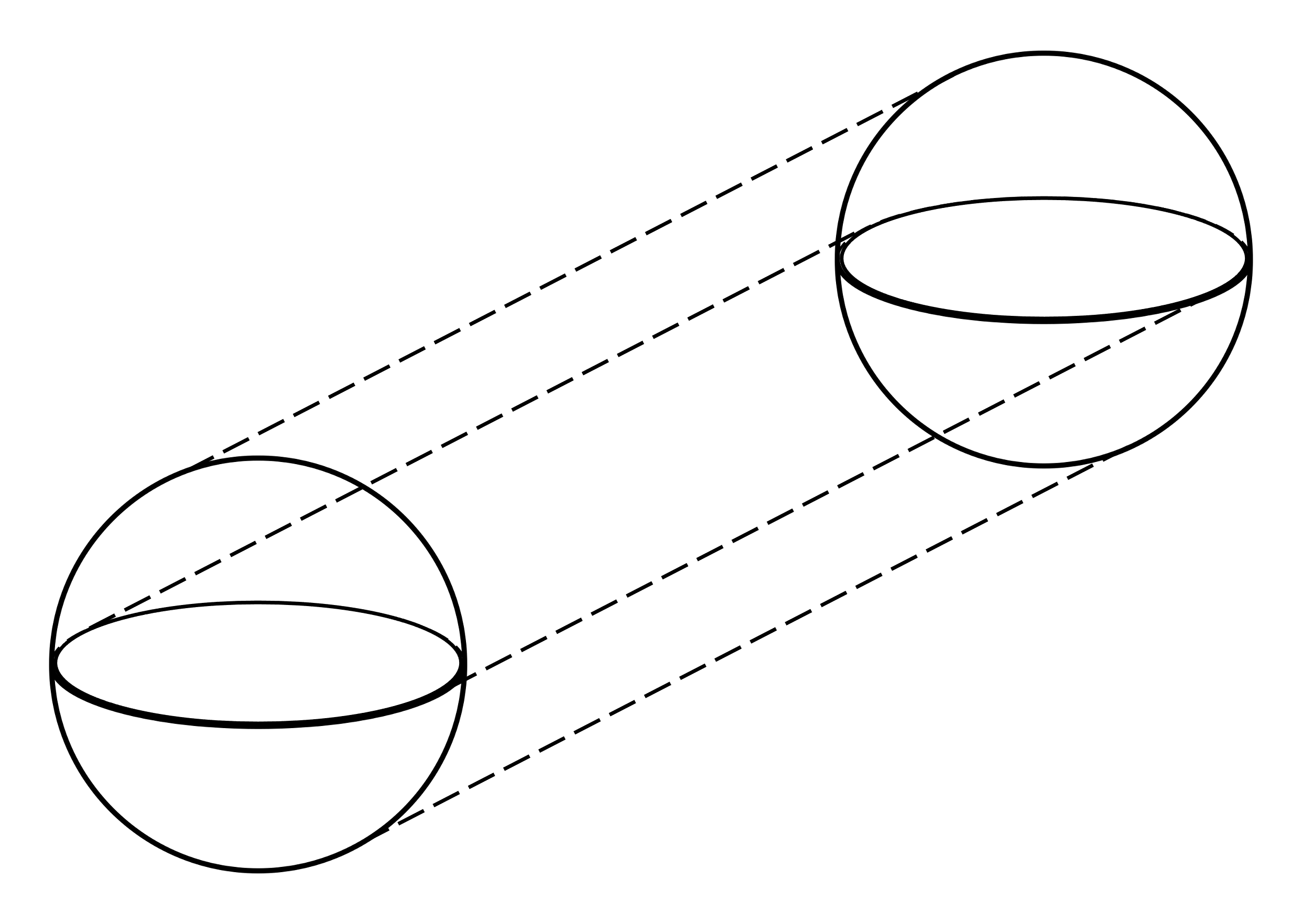
Figure 20: An illustration of the hypercylinder geometry. Note: this drawing is not to scale.

Mesh	Elements	Vertices
1	638	145
2	7,505	1,581
3	17,596	3,681
4	40,563	8,456
5	101,894	21,272
6	269,623	56,154

Table 5: The number of tetrahedral elements and vertices for a sequence of hypersurface meshes for the hypercylinder test case.

After the hypersurface meshes were generated, we proceeded to construct a family of hypervolume meshes which conformed (at least partially) to the hypersurface meshes. We note that boundary facets of the hypervolume meshes were not always guaranteed to coincide with boundary facets of the original hypersurface meshes, as we did not implement a boundary-recovery procedure for the work in this paper. Nevertheless, each hypervolume mesh conformed to the discrete representation of the hypercylinder geometry. This fact was guaranteed due to the convexity of the hypercylinder. The hypervolume meshes were generated by applying the point-insertion process (from Section 3) to each of the points in a given hypersurface mesh from Table 5. The resulting meshes were composed of pentatope elements, and the properties of each mesh are summarized in Table 6.

Mesh	Elements	Vertices
1	1,627	145
2	23,197	1,581
3	55,402	3,681
4	114,077	8,456
5	305,204	21,272
6	804,103	56,154

Table 6: The number of pentatope elements and vertices for a sequence of hypervolume meshes for the hypercylinder test case.

The ‘hypervolume error’ associated with each hypervolume mesh was calculated as follows

$$HV_{\mathrm{error}}=\left|HV_{\mathrm{exact}}-HV_{\mathrm{approx}}\right|,$$

where $HV_{\mathrm{exact}}$ is the exact hypercylinder hypervolume given by

$$HV_{\mathrm{exact}}=\frac{4}{3}\pi R^{3}L,$$

and $HV_{\mathrm{approx}}$ was the summation of the hypervolumes of the pentatopes in each mesh. Figure 21 shows a plot of the hypervolume error versus the characteristic mesh spacing. We estimated the characteristic mesh spacing by raising the total number of pentatope elements in each mesh to the -1/3 power. Based on the figure, we can clearly see that the hypervolume error converges at a rate of 2nd order. This is what we would expect when using straight-sided elements to approximate a curved surface.

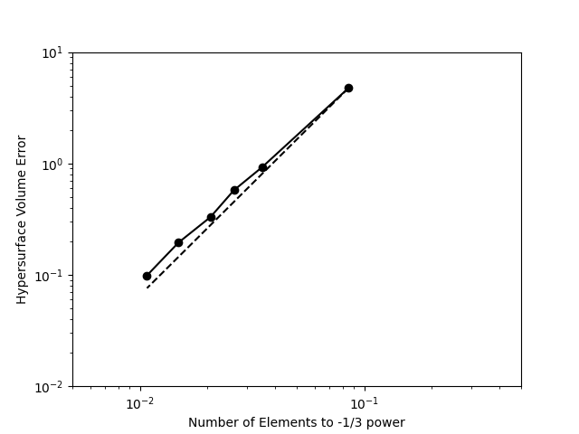
Figure 21: The plot above shows the hypervolume error, $HV_{\mathrm{error}}$, for the hypercylinder test case. The errors are plotted against the characteristic mesh spacing for a sequence of increasingly refined hypervolume meshes. In addition, a dashed line associated with 2nd-order convergence is plotted for reference.

6.2 Quality Improvement Study

For this numerical experiment, we generated sets of points distributed randomly within a tesseract domain. Thereafter, a mesh for these points was constructed using the Delaunay point-insertion algorithm of Section 3. Once a valid mesh containing all of the points was generated within the bounding tesseract, all pentatopes associated with the points from the bounding tesseract were removed, leaving a valid mesh consisting of only the randomly generated points.

Next, we analyzed the mesh, and the worst quality pentatope was identified and dubbed the starter pentatope. Then, all possible flips were determined based on its relationship with the set of all pentatopes that share at least one of its vertices. Of the valid flips, we identified those that increased the quality of the lowest quality element, and produced valid reconnections, (i.e. flips that preserve the hypervolume and do not introduce zero hypervolume elements). From this set of flips, the flip with the largest increase in quality of the lowest quality element was executed. It is worth noting that failing to find valid flips for a particular starter pentatope is a common occurrence. Any pentatopes resulting from a flip were frozen and no longer allowed to change. In addition, pentatopes chosen as the starter pentatope were logged in order to prevent them from being chosen a second time. Our algorithm terminated when all pentatopes were either frozen or already chosen as the starter pentatope in a previous iteration.

The tests were performed with small meshes of 50, 100, 150, 200, 250, and 300 points. The quality improvement algorithm was successfully employed on each mesh. In order to investigate the degree of quality improvement, the average quality of the worst ten percent of the total number of elements was calculated before and after executing the flips. The results are shown in Tables 7 and 8.

		No. Pentatopes		Hypervolume
No. Points	No. Flips	Initial	Final	Initial	Final
50	40	492	450	30,340,041.467995968	30,340,041.467995968
100	99	1,421	1,317	48,546,097.039964405	48,546,097.039964405
150	194	2,443	2,209	53,983,703.043834004	53,983,703.043834004
200	292	3,581	3,271	58,893,885.023952322	58,893,885.023952322
250	396	4,767	4,323	63,293,417.543503716	63,293,417.543503716
300	528	6,010	5,408	65,849,297.299100857	65,849,297.299100857

Table 7: Information for quality improvement cases on randomized meshes.

	Avg. Min. Quality
No. Points	Initial	Final
50	0.194	0.221
100	0.244	0.270
150	0.212	0.229
200	0.202	0.225
250	0.203	0.225
300	0.198	0.225

Table 8: Quality improvement results for randomized meshes.

The initial and final hypervolumes are consistent, before and after quality improvement operations have been attempted, which demonstrates the validity of the bistellar flips. In addition, the flips produce consistent improvement for low quality elements in each mesh. More complex algorithms associated with the bistellar flips may produce better results; however, the purpose of this numerical experiment is to simply demonstrate the validity of these flips and a potential use case.

7 Conclusion

A robust method for 4D point insertion has been presented along with explicit descriptions of orientation and in-hypersphere geometric predicates. In addition, a new set of quality metrics for pentatope elements, and 4D bistellar flips for groupings (collections) of multiple pentatope elements have been presented. Finally, our algorithms were verified using a pair of numerical experiments: i) the point-insertion algorithm was used to generate a family of hypervolume meshes for a hypercylinder geometry, and the hypervolume errors of these meshes were shown to converge at the expected rate; ii) an algorithm for quality improvement was developed using the bistellar flips, and this algorithm was shown to consistently raise the average quality of the worst elements in a series of randomized meshes.

In future work, 4D boundary recovery will be implemented in order to generate high-quality, constrained Delaunay boundary meshes. This will be an important endeavor, especially for hypervolume mesh generation on non-convex domains. The work carried out in this paper, e.g. developing a robust point-insertion algorithm and developing methods for mesh quality improvement, are important steps towards achieving the goal of fully-automatic and robust constrained hypervolume mesh generation in 4D.

Declaration of Competing Interests

The authors declare that they have no known competing financial interests or personal relationships that could have appeared to influence the work reported in this paper.

Funding

This research received funding from the United States Naval Research Laboratory (NRL) under grant number N00173-22-2-C008. In turn, the NRL grant itself was funded by Steven Martens, Program Officer for the Power, Propulsion and Thermal Management Program, Code 35, in the United States Office of Naval Research.

Appendix A Tesseract Subdivision

Pentatopes 1-26	Pentatopes 27-52	Pentatopes 53-78	Pentatopes 79-104
4 8 12 17 19	8 12 16 17 19	3 7 11 18 19	7 11 15 18 19
2 6 10 17 20	6 10 14 17 20	1 5 9 18 20	5 9 13 18 20
6 8 14 17 21	8 14 16 17 21	5 7 13 18 21	7 13 15 18 21
7 8 15 19 21	8 15 16 19 21	8 16 17 19 21	7 15 18 19 21
5 6 13 20 21	6 13 14 20 21	6 14 17 20 21	5 13 18 20 21
2 4 10 17 22	4 10 12 17 22	1 3 9 18 22	3 9 11 18 22
3 4 11 19 22	4 11 12 19 22	4 12 17 19 22	3 11 18 19 22
1 2 9 20 22	2 9 10 20 22	2 10 17 20 22	1 9 18 20 22
10 12 14 17 23	12 14 16 17 23	9 11 13 18 23	11 13 15 18 23
11 12 15 19 23	12 15 16 19 23	12 16 17 19 23	11 15 18 19 23
9 10 13 20 23	10 13 14 20 23	10 14 17 20 23	9 13 18 20 23
13 14 15 21 23	14 15 16 21 23	14 16 17 21 23	13 15 18 21 23
15 16 19 21 23	16 17 19 21 23	15 18 19 21 23	17 18 19 21 23
13 14 20 21 23	14 17 20 21 23	13 18 20 21 23	17 18 20 21 23
9 10 11 22 23	10 11 12 22 23	10 12 17 22 23	9 11 18 22 23
11 12 19 22 23	12 17 19 22 23	11 18 19 22 23	17 18 19 22 23
9 10 20 22 23	10 17 20 22 23	9 18 20 22 23	17 18 20 22 23
2 4 6 17 24	4 6 8 17 24	1 3 5 18 24	3 5 7 18 24
3 4 7 19 24	4 7 8 19 24	4 8 17 19 24	3 7 18 19 24
1 2 5 20 24	2 5 6 20 24	2 6 17 20 24	1 5 18 20 24
5 6 7 21 24	6 7 8 21 24	6 8 17 21 24	5 7 18 21 24
7 8 19 21 24	8 17 19 21 24	7 18 19 21 24	17 18 19 21 24
5 6 20 21 24	6 17 20 21 24	5 18 20 21 24	17 18 20 21 24
1 2 3 22 24	2 3 4 22 24	2 4 17 22 24	1 3 18 22 24
3 4 19 22 24	4 17 19 22 24	3 18 19 22 24	17 18 19 22 24
1 2 20 22 24	2 17 20 22 24	1 18 20 22 24	17 18 20 22 24

Table 9: Indices for the subdivision of the tesseract into $N_{b}=104$ pentatopes.

Appendix B Determinants

B.1 Orientation

This section contains the sub-determinants associated with the $5\times 5$ determinant that is required for the orientation calculation. A sequence of $2\times 2$ determinants can be computed based on values from the original $5\times 5$ determinant

$$ab =\begin{vmatrix}a_{x}&a_{y}\\ b_{x}&b_{y}\end{vmatrix}\quad bc=\begin{vmatrix}b_{x}&b_{y}\\ c_{x}&c_{y}\end{vmatrix}\quad cd=\begin{vmatrix}c_{x}&c_{y}\\ d_{x}&d_{y}\end{vmatrix}\quad de=\begin{vmatrix}d_{x}&d_{y}\\ e_{x}&e_{y}\end{vmatrix}\quad ea=\begin{vmatrix}e_{x}&e_{y}\\ a_{x}&a_{y}\end{vmatrix},$$

$$ac =\begin{vmatrix}a_{x}&a_{y}\\ c_{x}&c_{y}\end{vmatrix}\quad bd=\begin{vmatrix}b_{x}&b_{y}\\ d_{x}&d_{y}\end{vmatrix}\quad ce=\begin{vmatrix}c_{x}&c_{y}\\ e_{x}&e_{y}\end{vmatrix}\quad da=\begin{vmatrix}d_{x}&d_{y}\\ a_{x}&a_{y}\end{vmatrix}\quad eb=\begin{vmatrix}e_{x}&e_{y}\\ b_{x}&b_{y}\end{vmatrix}.$$

Next, a sequence of $3\times 3$ determinants can be computed based on the $2\times 2$ determinants

$$abc =\begin{vmatrix}a_{x}&a_{y}&a_{z}\\ b_{x}&b_{y}&b_{z}\\ c_{x}&c_{y}&c_{z}\end{vmatrix}=a_{z}(bc)-b_{z}(ac)+c_{z}(ab),\qquad bcd=\begin{vmatrix}b_{x}&b_{y}&b_{z}\\ c_{x}&c_{y}&c_{z}\\ d_{x}&d_{y}&d_{z}\end{vmatrix}=b_{z}(cd)-c_{z}(bd)+d_{z}(bc),$$

$$cde =\begin{vmatrix}c_{x}&c_{y}&c_{z}\\ d_{x}&d_{y}&d_{z}\\ e_{x}&e_{y}&e_{z}\end{vmatrix}=c_{z}(de)-d_{z}(ce)+e_{z}(cd),\qquad dea=\begin{vmatrix}d_{x}&d_{y}&d_{z}\\ e_{x}&e_{y}&e_{z}\\ a_{x}&a_{y}&a_{z}\end{vmatrix}=d_{z}(ea)-e_{z}(da)+a_{z}(de),$$

$$eab =\begin{vmatrix}e_{x}&e_{y}&e_{z}\\ a_{x}&a_{y}&a_{z}\\ b_{x}&b_{y}&b_{z}\end{vmatrix}=e_{z}(ab)-a_{z}(eb)+b_{z}(ea),\qquad abd=\begin{vmatrix}a_{x}&a_{y}&a_{z}\\ b_{x}&b_{y}&b_{z}\\ d_{x}&d_{y}&d_{z}\end{vmatrix}=a_{z}(bd)+b_{z}(da)+d_{z}(ab),$$

$$bce =\begin{vmatrix}b_{x}&b_{y}&b_{z}\\ c_{x}&c_{y}&c_{z}\\ e_{x}&e_{y}&e_{z}\end{vmatrix}=b_{z}(ce)+c_{z}(eb)+e_{z}(bc),\qquad cda=\begin{vmatrix}c_{x}&c_{y}&c_{z}\\ d_{x}&d_{y}&d_{z}\\ a_{x}&a_{y}&a_{z}\end{vmatrix}=c_{z}(da)+d_{z}(ac)+a_{z}(cd),$$

$$deb =\begin{vmatrix}d_{x}&d_{y}&d_{z}\\ e_{x}&e_{y}&e_{z}\\ b_{x}&b_{y}&b_{z}\end{vmatrix}=d_{z}(eb)+e_{z}(bd)+b_{z}(de),\qquad eac=\begin{vmatrix}e_{x}&e_{y}&e_{z}\\ a_{x}&a_{y}&a_{z}\\ c_{x}&c_{y}&c_{z}\end{vmatrix}=e_{z}(ac)+a_{z}(ce)+c_{z}(ea).$$

B.2 In-Hypersphere

This section contains the sub-determinants associated with the $6\times 6$ determinant that is required for the in-hypersphere calculation. A sequence of $2\times 2$ determinants can be computed based on values from the original $6\times 6$ determinant as follows

$$ab =\begin{vmatrix}a_{x}&a_{y}\\ b_{x}&b_{y}\end{vmatrix}\quad bc=\begin{vmatrix}b_{x}&b_{y}\\ c_{x}&c_{y}\end{vmatrix}\quad cd=\begin{vmatrix}c_{x}&c_{y}\\ d_{x}&d_{y}\end{vmatrix}\quad de=\begin{vmatrix}d_{x}&d_{y}\\ e_{x}&e_{y}\end{vmatrix}\quad ef=\begin{vmatrix}e_{x}&e_{y}\\ f_{x}&f_{y}\end{vmatrix},$$

$$fa =\begin{vmatrix}f_{x}&f_{y}\\ a_{x}&a_{y}\end{vmatrix}\quad ac=\begin{vmatrix}a_{x}&a_{y}\\ c_{x}&c_{y}\end{vmatrix}\quad bd=\begin{vmatrix}b_{x}&b_{y}\\ d_{x}&d_{y}\end{vmatrix}\quad ce=\begin{vmatrix}c_{x}&c_{y}\\ e_{x}&e_{y}\end{vmatrix}\quad df=\begin{vmatrix}d_{x}&d_{y}\\ f_{x}&f_{y}\end{vmatrix},$$

$$ea =\begin{vmatrix}e_{x}&e_{y}\\ a_{x}&a_{y}\end{vmatrix}\quad fb=\begin{vmatrix}f_{x}&f_{y}\\ b_{x}&b_{y}\end{vmatrix}\quad ad=\begin{vmatrix}a_{x}&a_{y}\\ d_{x}&d_{y}\end{vmatrix}\quad be=\begin{vmatrix}b_{x}&b_{y}\\ e_{x}&e_{y}\end{vmatrix}\quad cf=\begin{vmatrix}c_{x}&c_{y}\\ f_{x}&f_{y}\end{vmatrix}.$$

Next, a sequence of $3\times 3$ determinants can be computed based on the $2\times 2$ determinants.

$$abc =\begin{vmatrix}a_{x}&a_{y}&a_{z}\\ b_{x}&b_{y}&b_{z}\\ c_{x}&c_{y}&c_{z}\end{vmatrix}=a_{z}(bc)-b_{z}(ac)+c_{z}(ab),\qquad bcd=\begin{vmatrix}b_{x}&b_{y}&b_{z}\\ c_{x}&c_{y}&c_{z}\\ d_{x}&d_{y}&d_{z}\end{vmatrix}=b_{z}(cd)-c_{z}(bd)+d_{z}(bc),$$

$$cde =\begin{vmatrix}c_{x}&c_{y}&c_{z}\\ d_{x}&d_{y}&d_{z}\\ e_{x}&e_{y}&e_{z}\end{vmatrix}=c_{z}(de)-d_{z}(ce)+e_{z}(cd),\qquad def=\begin{vmatrix}d_{x}&d_{y}&d_{z}\\ e_{x}&e_{y}&e_{z}\\ f_{x}&f_{y}&f_{z}\end{vmatrix}=d_{z}(ef)-e_{z}(df)+f_{z}(de),$$

$$efa =\begin{vmatrix}e_{x}&e_{y}&e_{z}\\ f_{x}&f_{y}&f_{z}\\ a_{x}&a_{y}&a_{z}\end{vmatrix}=e_{z}(fa)-f_{z}(ea)+a_{z}(ef),\qquad fab=\begin{vmatrix}f_{x}&f_{y}&f_{z}\\ a_{x}&a_{y}&a_{z}\\ b_{x}&b_{y}&b_{z}\end{vmatrix}=f_{z}(ab)-a_{z}(fb)+b_{z}(fa),$$

$$abd =\begin{vmatrix}a_{x}&a_{y}&a_{z}\\ b_{x}&b_{y}&b_{z}\\ d_{x}&d_{y}&d_{z}\end{vmatrix}=a_{z}(bd)-b_{z}(ad)+d_{z}(ab),\qquad bce=\begin{vmatrix}b_{x}&b_{y}&b_{z}\\ c_{x}&c_{y}&c_{z}\\ e_{x}&e_{y}&e_{z}\end{vmatrix}=b_{z}(ce)-c_{z}(be)+e_{z}(bc),$$

$$cdf =\begin{vmatrix}c_{x}&c_{y}&c_{z}\\ d_{x}&d_{y}&d_{z}\\ f_{x}&f_{y}&f_{z}\end{vmatrix}=c_{z}(df)-d_{z}(cf)+f_{z}(cd),\qquad dea=\begin{vmatrix}d_{x}&d_{y}&d_{z}\\ e_{x}&e_{y}&e_{z}\\ a_{x}&a_{y}&a_{z}\end{vmatrix}=d_{z}(ea)+e_{z}(ad)+a_{z}(de),$$

$$efb =\begin{vmatrix}e_{x}&e_{y}&e_{z}\\ f_{x}&f_{y}&f_{z}\\ b_{x}&b_{y}&b_{z}\end{vmatrix}=e_{z}(fb)+f_{z}(be)+b_{z}(ef),\qquad fac=\begin{vmatrix}f_{x}&f_{y}&f_{z}\\ a_{x}&a_{y}&a_{z}\\ c_{x}&c_{y}&c_{z}\end{vmatrix}=f_{z}(ac)+a_{z}(cf)+c_{z}(fa),$$

$$abe =\begin{vmatrix}a_{x}&a_{y}&a_{z}\\ b_{x}&b_{y}&b_{z}\\ e_{x}&e_{y}&e_{z}\end{vmatrix}=a_{z}(be)+b_{z}(ea)+e_{z}(ab),\qquad bcf=\begin{vmatrix}b_{x}&b_{y}&b_{z}\\ c_{x}&c_{y}&c_{z}\\ f_{x}&f_{y}&f_{z}\end{vmatrix}=b_{z}(cf)+c_{z}(fb)+f_{z}(bc),$$

$$cda =\begin{vmatrix}c_{x}&c_{y}&c_{z}\\ d_{x}&d_{y}&d_{z}\\ a_{x}&a_{y}&a_{z}\end{vmatrix}=-c_{z}(ad)+d_{z}(ac)+a_{z}(cd),\qquad deb=\begin{vmatrix}d_{x}&d_{y}&d_{z}\\ e_{x}&e_{y}&e_{z}\\ b_{x}&b_{y}&b_{z}\end{vmatrix}=-d_{z}(be)+e_{z}(bd)+b_{z}(de),$$

$$efc =\begin{vmatrix}e_{x}&e_{y}&e_{z}\\ f_{x}&f_{y}&f_{z}\\ c_{x}&c_{y}&c_{z}\end{vmatrix}=-e_{z}(cf)+f_{z}(ce)+c_{z}(ef),\qquad ace=\begin{vmatrix}a_{x}&a_{y}&a_{z}\\ c_{x}&c_{y}&c_{z}\\ e_{x}&e_{y}&e_{z}\end{vmatrix}=a_{z}(ce)+c_{z}(ea)+e_{z}(ac),$$

$$bdf =\begin{vmatrix}b_{x}&b_{y}&b_{z}\\ d_{x}&d_{y}&d_{z}\\ f_{x}&f_{y}&f_{z}\end{vmatrix}=b_{z}(df)+d_{z}(fb)+f_{z}(bd),\qquad fad=\begin{vmatrix}f_{x}&f_{y}&f_{z}\\ a_{x}&a_{y}&a_{z}\\ d_{x}&d_{y}&d_{z}\end{vmatrix}=f_{z}(ad)+a_{z}(df)+d_{z}(fa).$$

Thereafter, a sequence of $4\times 4$ determinants can be computed based on the $3\times 3$ determinants

$$abcd =\begin{vmatrix}a_{x}&a_{y}&a_{z}&a_{t}\\ b_{x}&b_{y}&b_{z}&b_{t}\\ c_{x}&c_{y}&c_{z}&c_{t}\\ d_{x}&d_{y}&d_{z}&d_{t}\end{vmatrix}=-a_{t}(bcd)+b_{t}(cda)-c_{t}(abd)+d_{t}(abc),$$

$$bcde =\begin{vmatrix}b_{x}&b_{y}&b_{z}&b_{t}\\ c_{x}&c_{y}&c_{z}&c_{t}\\ d_{x}&d_{y}&d_{z}&d_{t}\\ e_{x}&e_{y}&e_{z}&e_{t}\end{vmatrix}=-b_{t}(cde)+c_{t}(deb)-d_{t}(bce)+e_{t}(bcd),$$

$$cdef =\begin{vmatrix}c_{x}&c_{y}&c_{z}&c_{t}\\ d_{x}&d_{y}&d_{z}&d_{t}\\ e_{x}&e_{y}&e_{z}&e_{t}\\ f_{x}&f_{y}&f_{z}&f_{t}\end{vmatrix}=-c_{t}(def)+d_{t}(efc)-e_{t}(cdf)+f_{t}(cde),$$

$$defa =\begin{vmatrix}d_{x}&d_{y}&d_{z}&d_{t}\\ e_{x}&e_{y}&e_{z}&e_{t}\\ f_{x}&f_{y}&f_{z}&f_{t}\\ a_{x}&a_{y}&a_{z}&a_{t}\end{vmatrix}=-d_{t}(efa)+e_{t}(fad)-f_{t}(dea)+a_{t}(def),$$

$$efab =\begin{vmatrix}e_{x}&e_{y}&e_{z}&e_{t}\\ f_{x}&f_{y}&f_{z}&f_{t}\\ a_{x}&a_{y}&a_{z}&a_{t}\\ b_{x}&b_{y}&b_{z}&b_{t}\end{vmatrix}=-e_{t}(fab)+f_{t}(abe)-a_{t}(efb)+b_{t}(efa),$$

$$fabc =\begin{vmatrix}f_{x}&f_{y}&f_{z}&f_{t}\\ a_{x}&a_{y}&a_{z}&a_{t}\\ b_{x}&b_{y}&b_{z}&b_{t}\\ c_{x}&c_{y}&c_{z}&c_{t}\end{vmatrix}=-f_{t}(abc)+a_{t}(bcf)-b_{t}(fac)+c_{t}(fab),$$

$$abce =\begin{vmatrix}a_{x}&a_{y}&a_{z}&a_{t}\\ b_{x}&b_{y}&b_{z}&b_{t}\\ c_{x}&c_{y}&c_{z}&c_{t}\\ e_{x}&e_{y}&e_{z}&e_{t}\end{vmatrix}=-a_{t}(bce)+b_{t}(ace)-c_{t}(abe)+e_{t}(abc),$$

$$bcdf =\begin{vmatrix}b_{x}&b_{y}&b_{z}&b_{t}\\ c_{x}&c_{y}&c_{z}&c_{t}\\ d_{x}&d_{y}&d_{z}&d_{t}\\ f_{x}&f_{y}&f_{z}&f_{t}\end{vmatrix}=-b_{t}(cdf)+c_{t}(bdf)-d_{t}(bcf)+f_{t}(bcd),$$

$$cdea =\begin{vmatrix}c_{x}&c_{y}&c_{z}&c_{t}\\ d_{x}&d_{y}&d_{z}&d_{t}\\ e_{x}&e_{y}&e_{z}&e_{t}\\ a_{x}&a_{y}&a_{z}&a_{t}\end{vmatrix}=-c_{t}(dea)+d_{t}(ace)-e_{t}(cda)+a_{t}(cde),$$

$$defb =\begin{vmatrix}d_{x}&d_{y}&d_{z}&d_{t}\\ e_{x}&e_{y}&e_{z}&e_{t}\\ f_{x}&f_{y}&f_{z}&f_{t}\\ b_{x}&b_{y}&b_{z}&b_{t}\end{vmatrix}=-d_{t}(efb)+e_{t}(bdf)-f_{t}(deb)+b_{t}(def),$$

$$efac =\begin{vmatrix}e_{x}&e_{y}&e_{z}&e_{t}\\ f_{x}&f_{y}&f_{z}&f_{t}\\ a_{x}&a_{y}&a_{z}&a_{t}\\ c_{x}&c_{y}&c_{z}&c_{t}\end{vmatrix}=-e_{t}(fac)+f_{t}(ace)-a_{t}(efc)+c_{t}(efa),$$

$$fabd =\begin{vmatrix}f_{x}&f_{y}&f_{z}&f_{t}\\ a_{x}&a_{y}&a_{z}&a_{t}\\ b_{x}&b_{y}&b_{z}&b_{t}\\ d_{x}&d_{y}&d_{z}&d_{t}\end{vmatrix}=-f_{t}(abd)+a_{t}(bdf)-b_{t}(fad)+d_{t}(fab),$$

$$abde =\begin{vmatrix}a_{x}&a_{y}&a_{z}&a_{t}\\ b_{x}&b_{y}&b_{z}&b_{t}\\ d_{x}&d_{y}&d_{z}&d_{t}\\ e_{x}&e_{y}&e_{z}&e_{t}\end{vmatrix}=-a_{t}(deb)+b_{t}(dea)-d_{t}(abe)+e_{t}(abd),$$

$$bcef =\begin{vmatrix}b_{x}&b_{y}&b_{z}&b_{t}\\ c_{x}&c_{y}&c_{z}&c_{t}\\ e_{x}&e_{y}&e_{z}&e_{t}\\ f_{x}&f_{y}&f_{z}&f_{t}\end{vmatrix}=-b_{t}(efc)+c_{t}(efb)-e_{t}(bcf)+f_{t}(bce),$$

$$cdfa =\begin{vmatrix}c_{x}&c_{y}&c_{z}&c_{t}\\ d_{x}&d_{y}&d_{z}&d_{t}\\ f_{x}&f_{y}&f_{z}&f_{t}\\ a_{x}&a_{y}&a_{z}&a_{t}\end{vmatrix}=-c_{t}(fad)+d_{t}(fac)-f_{t}(cda)+a_{t}(cdf).$$

Finally, a sequence of $5\times 5$ determinants can be computed based on the $4\times 4$ determinants

$$abcde =\begin{vmatrix}a_{x}&a_{y}&a_{z}&a_{t}&a_{x}^{2}+a_{y}^{2}+a_{z}^{2}+a_{t}^{2}\\ b_{x}&b_{y}&b_{z}&b_{t}&b_{x}^{2}+b_{y}^{2}+b_{z}^{2}+b_{t}^{2}\\ c_{x}&c_{y}&c_{z}&c_{t}&c_{x}^{2}+c_{y}^{2}+c_{z}^{2}+c_{t}^{2}\\ d_{x}&d_{y}&d_{z}&d_{t}&d_{x}^{2}+d_{y}^{2}+d_{z}^{2}+d_{t}^{2}\\ e_{x}&e_{y}&e_{z}&e_{t}&e_{x}^{2}+e_{y}^{2}+e_{z}^{2}+e_{t}^{2}\end{vmatrix}$$

$$=(a_{x}^{2}+a_{y}^{2}+a_{z}^{2}+a_{t}^{2})(bcde)+(b_{x}^{2}+b_{y}^{2}+b_{z}^{2}+b_{t}^{2})(cdea)+(c_{x}^{2}+c_{y}^{2}+c_{z}^{2}+c_{t}^{2})(abde)$$

$$-(d_{x}^{2}+d_{y}^{2}+d_{z}^{2}+d_{t}^{2})(abce)+(e_{x}^{2}+e_{y}^{2}+e_{z}^{2}+e_{t}^{2})(abcd),$$

$$bcdef =\begin{vmatrix}b_{x}&b_{y}&b_{z}&b_{t}&b_{x}^{2}+b_{y}^{2}+b_{z}^{2}+b_{t}^{2}\\ c_{x}&c_{y}&c_{z}&c_{t}&c_{x}^{2}+c_{y}^{2}+c_{z}^{2}+c_{t}^{2}\\ d_{x}&d_{y}&d_{z}&d_{t}&d_{x}^{2}+d_{y}^{2}+d_{z}^{2}+d_{t}^{2}\\ e_{x}&e_{y}&e_{z}&e_{t}&e_{x}^{2}+e_{y}^{2}+e_{z}^{2}+e_{t}^{2}\\ f_{x}&f_{y}&f_{z}&f_{t}&f_{x}^{2}+f_{y}^{2}+f_{z}^{2}+f_{t}^{2}\end{vmatrix}$$

$$=(b_{x}^{2}+b_{y}^{2}+b_{z}^{2}+b_{t}^{2})(cdef)+(c_{x}^{2}+c_{y}^{2}+c_{z}^{2}+c_{t}^{2})(defb)+(d_{x}^{2}+d_{y}^{2}+d_{z}^{2}+d_{t}^{2})(bcef)$$

$$-(e_{x}^{2}+e_{y}^{2}+e_{z}^{2}+e_{t}^{2})(bcdf)+(f_{x}^{2}+f_{y}^{2}+f_{z}^{2}+f_{t}^{2})(bcde),$$

$$cdefa =\begin{vmatrix}c_{x}&c_{y}&c_{z}&c_{t}&c_{x}^{2}+c_{y}^{2}+c_{z}^{2}+c_{t}^{2}\\ d_{x}&d_{y}&d_{z}&d_{t}&d_{x}^{2}+d_{y}^{2}+d_{z}^{2}+d_{t}^{2}\\ e_{x}&e_{y}&e_{z}&e_{t}&e_{x}^{2}+e_{y}^{2}+e_{z}^{2}+e_{t}^{2}\\ f_{x}&f_{y}&f_{z}&f_{t}&f_{x}^{2}+f_{y}^{2}+f_{z}^{2}+f_{t}^{2}\\ a_{x}&a_{y}&a_{z}&a_{t}&a_{x}^{2}+a_{y}^{2}+a_{z}^{2}+a_{t}^{2}\end{vmatrix}$$

$$=(c_{x}^{2}+c_{y}^{2}+c_{z}^{2}+c_{t}^{2})(defa)+(d_{x}^{2}+d_{y}^{2}+d_{z}^{2}+d_{t}^{2})(efac)+(e_{x}^{2}+e_{y}^{2}+e_{z}^{2}+e_{t}^{2})(cdfa)$$

$$-(f_{x}^{2}+f_{y}^{2}+f_{z}^{2}+f_{t}^{2})(cdea)+(a_{x}^{2}+a_{y}^{2}+a_{z}^{2}+a_{t}^{2})(cdef),$$

$$defab =\begin{vmatrix}d_{x}&d_{y}&d_{z}&d_{t}&d_{x}^{2}+d_{y}^{2}+d_{z}^{2}+d_{t}^{2}\\ e_{x}&e_{y}&e_{z}&e_{t}&e_{x}^{2}+e_{y}^{2}+e_{z}^{2}+e_{t}^{2}\\ f_{x}&f_{y}&f_{z}&f_{t}&f_{x}^{2}+f_{y}^{2}+f_{z}^{2}+f_{t}^{2}\\ a_{x}&a_{y}&a_{z}&a_{t}&a_{x}^{2}+a_{y}^{2}+a_{z}^{2}+a_{t}^{2}\\ b_{x}&b_{y}&b_{z}&b_{t}&b_{x}^{2}+b_{y}^{2}+b_{z}^{2}+b_{t}^{2}\end{vmatrix}$$

$$=(d_{x}^{2}+d_{y}^{2}+d_{z}^{2}+d_{t}^{2})(efab)+(e_{x}^{2}+e_{y}^{2}+e_{z}^{2}+e_{t}^{2})(fabd)+(f_{x}^{2}+f_{y}^{2}+f_{z}^{2}+f_{t}^{2})(abde)$$

$$-(a_{x}^{2}+a_{y}^{2}+a_{z}^{2}+a_{t}^{2})(defb)+(b_{x}^{2}+b_{y}^{2}+b_{z}^{2}+b_{t}^{2})(defa),$$

$$efabc =\begin{vmatrix}e_{x}&e_{y}&e_{z}&e_{t}&e_{x}^{2}+e_{y}^{2}+e_{z}^{2}+e_{t}^{2}\\ f_{x}&f_{y}&f_{z}&f_{t}&f_{x}^{2}+f_{y}^{2}+f_{z}^{2}+f_{t}^{2}\\ a_{x}&a_{y}&a_{z}&a_{t}&a_{x}^{2}+a_{y}^{2}+a_{z}^{2}+a_{t}^{2}\\ b_{x}&b_{y}&b_{z}&b_{t}&b_{x}^{2}+b_{y}^{2}+b_{z}^{2}+b_{t}^{2}\\ c_{x}&c_{y}&c_{z}&c_{t}&c_{x}^{2}+c_{y}^{2}+c_{z}^{2}+c_{t}^{2}\end{vmatrix}$$

$$=(e_{x}^{2}+e_{y}^{2}+e_{z}^{2}+e_{t}^{2})(fabc)+(f_{x}^{2}+f_{y}^{2}+f_{z}^{2}+f_{t}^{2})(abce)+(a_{x}^{2}+a_{y}^{2}+a_{z}^{2}+a_{t}^{2})(bcef)$$

$$-(b_{x}^{2}+b_{y}^{2}+b_{z}^{2}+b_{t}^{2})(efac)+(c_{x}^{2}+c_{y}^{2}+c_{z}^{2}+c_{t}^{2})(efab),$$

$$fabcd =\begin{vmatrix}f_{x}&f_{y}&f_{z}&f_{t}&f_{x}^{2}+f_{y}^{2}+f_{z}^{2}+f_{t}^{2}\\ a_{x}&a_{y}&a_{z}&a_{t}&a_{x}^{2}+a_{y}^{2}+a_{z}^{2}+a_{t}^{2}\\ b_{x}&b_{y}&b_{z}&b_{t}&b_{x}^{2}+b_{y}^{2}+b_{z}^{2}+b_{t}^{2}\\ c_{x}&c_{y}&c_{z}&c_{t}&c_{x}^{2}+c_{y}^{2}+c_{z}^{2}+c_{t}^{2}\\ d_{x}&d_{y}&d_{z}&d_{t}&d_{x}^{2}+d_{y}^{2}+d_{z}^{2}+d_{t}^{2}\end{vmatrix}$$

$$=(f_{x}^{2}+f_{y}^{2}+f_{z}^{2}+f_{t}^{2})(abcd)+(a_{x}^{2}+a_{y}^{2}+a_{z}^{2}+a_{t}^{2})(bcdf)+(b_{x}^{2}+b_{y}^{2}+b_{z}^{2}+b_{t}^{2})(cdfa)$$

$$-(c_{x}^{2}+c_{y}^{2}+c_{z}^{2}+c_{t}^{2})(fabd)+(d_{x}^{2}+d_{y}^{2}+d_{z}^{2}+d_{t}^{2})(fabc).$$

References

• [1] R. Löhner, P. Parikh, Generation of three-dimensional unstructured grids by the advancing-front method, International Journal for Numerical Methods in Fluids 8 (10) (1988) 1135–1149.
• [2] P. L. George, É. Seveno, The advancing-front mesh generation method revisited, International Journal for Numerical Methods in Engineering 37 (21) (1994) 3605–3619.
• [3] S. Hang, TetGen, a Delaunay-based quality tetrahedral mesh generator, ACM Trans. Math. Softw 41 (2) (2015) 11.
• [4] C. Gruau, T. Coupez, 3D tetrahedral, unstructured and anisotropic mesh generation with adaptation to natural and multidomain metric, Computer Methods in Applied Mechanics and Engineering 194 (48-49) (2005) 4951–4976.
• [5] D. J. Mavriplis, An advancing front Delaunay triangulation algorithm designed for robustness, Journal of Computational Physics 117 (1) (1995) 90–101.
• [6] P. J. Frey, H. Borouchaki, P.-L. George, 3D Delaunay mesh generation coupled with an advancing-front approach, Computer Methods in Applied Mechanics and Engineering 157 (1-2) (1998) 115–131.
• [7] A. Bowyer, Computing Dirichlet tessellations, The Computer Journal 24 (2) (1981) 162–166.
• [8] D. F. Watson, Computing the n-dimensional Delaunay tessellation with application to Voronoi polytopes, The Computer Journal 24 (2) (1981) 167–172.
• [9] D. S. Lo, Finite element mesh generation, CRC Press, 2014.
• [10] S.-W. Cheng, T. K. Dey, J. Shewchuk, S. Sahni, Delaunay mesh generation, CRC Press Boca Raton, 2013.
• [11] M. Behr, Simplex space–time meshes in finite element simulations, International Journal for Numerical Methods in Fluids 57 (9) (2008) 1421–1434.
• [12] L. Pauli, M. Behr, On stabilized space-time FEM for anisotropic meshes: Incompressible Navier–Stokes equations and applications to blood flow in medical devices, International Journal for Numerical Methods in Fluids 85 (3) (2017) 189–209.
• [13] M. von Danwitz, V. Karyofylli, N. Hosters, M. Behr, Simplex space-time meshes in compressible flow simulations, International Journal for Numerical Methods in Fluids 91 (1) (2019) 29–48.
• [14] V. Karyofylli, L. Wendling, M. Make, N. Hosters, M. Behr, Simplex space-time meshes in thermally coupled two-phase flow simulations of mold filling, Computers & Fluids 192 (2019) 104261.
• [15] M. Make, T. Spenke, N. Hosters, M. Behr, Spline-based space-time finite element approach for fluid-structure interaction problems with a focus on fully enclosed domains, Computers & Mathematics with Applications 114 (2022) 210–224.
• [16] M. Von Danwitz, I. Voulis, N. Hosters, M. Behr, Time-continuous and time-discontinuous space-time finite elements for advection-diffusion problems, International Journal for Numerical Methods in Engineering 124 (14) (2023) 3117–3144.
• [17] E. Karabelas, M. Neumüller, Generating admissible space-time meshes for moving domains in $d+1$-dimensions, arXiv preprint arXiv:1505.03973.
• [18] C. Lehrenfeld, The Nitsche XFEM-DG space-time method and its implementation in three space dimensions, SIAM Journal on Scientific Computing 37 (1) (2015) A245–A270.
• [19] M. von Danwitz, P. Antony, F. Key, N. Hosters, M. Behr, Four-dimensional elastically deformed simplex space-time meshes for domains with time-variant topology, International Journal for Numerical Methods in Fluids 93 (12) (2021) 3490–3506.
• [20] V. Karyofylli, M. Behr, Simplex space-time meshes in engineering applications with moving domains, arXiv preprint arXiv:2210.09831.
• [21] K. Takizawa, T. E. Tezduyar, Space–time flow computation with boundary layer and contact representation: a 10-year history, Computational Mechanics (2023) 1–30.
• [22] L. Wang, P.-O. Persson, A high-order discontinuous Galerkin method with unstructured space–time meshes for two-dimensional compressible flows on domains with large deformations, Computers & Fluids 118 (2015) 53–68.
• [23] L. Wang, Discontinuous Galerkin methods on moving domains with large deformations, Ph.D. thesis, University of California, Berkeley (2015).
• [24] T. L. Horváth, S. Rhebergen, A conforming sliding mesh technique for an embedded-hybridized discontinuous Galerkin discretization for fluid-rigid body interaction, International Journal for Numerical Methods in Fluids 94 (11) (2022) 1784–1809.
• [25] A. Üngör, A. Sheffer, Pitching tents in space-time: Mesh generation for discontinuous Galerkin method, International Journal of Foundations of Computer Science 13 (02) (2002) 201–221.
• [26] J. Erickson, D. Guoy, J. M. Sullivan, A. Üngör, Building spacetime meshes over arbitrary spatial domains, Engineering with Computers 20 (4) (2005) 342–353.
• [27] R. Abedi, S.-H. Chung, J. Erickson, Y. Fan, M. Garland, D. Guoy, R. Haber, J. M. Sullivan, S. Thite, Y. Zhou, Spacetime meshing with adaptive refinement and coarsening, in: Proceedings of the Twentieth Annual Symposium on Computational Geometry, 2004, pp. 300–309.
• [28] J. Gopalakrishnan, P. Monk, P. Sepúlveda, A tent pitching scheme motivated by Friedrichs theory, Computers & Mathematics with Applications 70 (5) (2015) 1114–1135.
• [29] J. Gopalakrishnan, J. Schöberl, C. Wintersteiger, Mapped tent pitching schemes for hyperbolic systems, SIAM Journal on Scientific Computing 39 (6) (2017) B1043–B1063.
• [30] D. Drake, J. Gopalakrishnan, J. Schöberl, C. Wintersteiger, Convergence analysis of some tent-based schemes for linear hyperbolic systems, Mathematics of Computation 91 (334) (2022) 699–733.
• [31] J. Gopalakrishnan, M. Hochsteger, J. Schöberl, C. Wintersteiger, An explicit mapped tent pitching scheme for Maxwell equations, in: Spectral and high order methods for partial differential equations – ICOSAHOM 2018, 2020, pp. 359–369.
• [32] P. Foteinos, N. Chrisochoides, 4D space–time Delaunay meshing for medical images, Engineering with Computers 31 (3) (2015) 499–511.
• [33] P. C. Caplan, R. Haimes, D. L. Darmofal, M. C. Galbraith, Four-dimensional anisotropic mesh adaptation, Computer-Aided Design 129 (2020) 102915.
• [34] M. Neumüller, O. Steinbach, Refinement of flexible space–time finite element meshes and discontinuous Galerkin methods, Computing and Visualization in Science 14 (5) (2011) 189–205.
• [35] G. Belda-Ferrín, E. Ruiz-Gironés, A. Gargallo-Peiró, X. Roca, Conformal marked bisection for local refinement of n-dimensional unstructured simplicial meshes, Computer-Aided Design 154 (2023) 103419.
• [36] P. C. D. Caplan, Four-dimensional anisotropic mesh adaptation for spacetime numerical simulations, Ph.D. thesis, Massachusetts Institute of Technology (2019).
• [37] J. T. Anderson, D. M. Williams, A. Corrigan, Surface and hypersurface meshing techniques for space-time finite element methods, Computer-Aided Design (2023) 103574.
• [38] A. D. Kercher, A. Corrigan, D. A. Kessler, The moving discontinuous Galerkin finite element method with interface condition enforcement for compressible viscous flows, International Journal for Numerical Methods in Fluids 93 (5) (2021) 1490–1519.
• [39] H. S. Coxeter, Discrete groups generated by reflections, Annals of Mathematics (1934) 588–621.
• [40] H. Freudenthal, Simplizialzerlegungen von beschrankter flachheit, Annals of Mathematics (1942) 580–582.
• [41] H. W. Kuhn, Some combinatorial lemmas in topology, IBM Journal of research and development 4 (5) (1960) 518–524.
• [42] R. W. Shores, E. J. Wegman, Bounds on Delaunay tessellations, Wiley Interdisciplinary Reviews: Computational Statistics 2 (5) (2010) 571–580.
• [43] J. R. Shewchuk, Adaptive precision floating-point arithmetic and fast robust geometric predicates, Tech. rep., Carnegie-Mellon University Pittsburgh Pennsylvania Department of Computer Science (1996).
• [44] J.-D. Boissonnat, O. Devillers, S. Hornus, Incremental construction of the Delaunay triangulation and the Delaunay graph in medium dimension, in: Proceedings of the twenty-fifth annual symposium on Computational geometry, 2009, pp. 208–216.
• [45] V. Dyedov, N. Ray, D. Einstein, X. Jiao, T. J. Tautges, AHF: Array-based half-facet data structure for mixed-dimensional and non-manifold meshes, Engineering with Computers 31 (2015) 389–404.
• [46] A. Liu, B. Joe, On the shape of tetrahedra from bisection, Mathematics of Computation 63 (207) (1994) 141–154.
• [47] J. R. Shewchuk, Updating and constructing constrained Delaunay and constrained regular triangulations by flips, in: Proceedings of the Nineteenth Annual Symposium on Computational Geometry, 2003, pp. 181–190.
• [48] A. Banburski, L.-Q. Chen, L. Freidel, J. Hnybida, Pachner moves in a 4d Riemannian holomorphic Spin Foam model, Physical Review D 92 (12) (2015) 124014.
• [49] A. Corrigan, A. Kercher, D. Kessler, The moving discontinuous Galerkin method with interface condition enforcement for unsteady three-dimensional flows, in: AIAA (Ed.), 2019 AIAA SciTech Forum, 2019, AIAA-2019-0642. doi:10.2514/6.2019-0642.