Construction of invariant curves for some planar Piecewise Isometries

Abstract.

We establish the existence of a family of piecewise linear invariant curves in a two-parameter family of piecewise isometries on the upper half-plane which are embeddings of interval exchange transformations and give rise to layers of invariant regions. We note that the restriction of the piecewise isometry to the union of these regions is a piecewise isometry that contains non-convex atoms, though we conjecture that the non-convexity does not have a pathological effect on the uniqueness of cell encodings in this case. We also show the existence of a trapezoidal piecewise isometry for which the dynamics on the top and bottom edges are distinct 2-interval exchange transformations.

1. Introduction

An interval exchange transformation (IET) is a pair $(\mathcal{I},f)$, which can be seen as a bijective piecewise translation of an interval $I=[a,b)\subset\mathbb{R}$. In particular, let $\mathcal{I}$ denote a partition of $I$ into $d\geq 2$ subintervals $I_{\alpha}$, indexed by an alphabet $\mathcal{A}$ of $d$ letters, and define $f:I\rightarrow I$ to be a bijection on $I$ so that the restriction of $f$ to each subinterval $I_{\alpha}\in\mathcal{I}$ is a translation. An IET $(\mathcal{I},f)$ is determined by a vector $\lambda\in\mathbb{R}_{+}^{\mathcal{A}}$, with coordinates $\lambda_{\alpha}$ (the lengths of the subintervals $I_{\alpha}$), and an irreducible permutation $\pi$ (describing the ordering of the subintervals before and after applying $f$). It is usual to write $f=f_{\lambda,\pi}$ and denote an IET by the pair $(I,f_{\lambda,\pi})$. Interval exchanges have been thoroughly studied and have a rich theory, see for instance [15, 16, 18, 19, 22], they generalise circle rotations and many related concepts, such as Lagrange’s Theorem [10], continued fractions and the Gauss map [21], Khinchin’s Theorem [24] and Sturmian shifts [23], and they have deep connections in the study of measured foliations and translation surfaces [20].

Piecewise isometries (PWIs) are a generalisation of IETs to higher dimensions and arbitrary metric spaces, consisting of a partition of the metric space into convex pieces, and a map which acts on the pieces by an isometry. The phase space can be naturally divided into two (or three) subsets, the exceptional set - consisting of the orbit of the discontinuity and the orbits which accumulate on it - and its complement, the regular set - consisting of a packing of convex periodic islands; many authors choose to distinguish the discontinuities from the orbits accumulating on it. One of the largest outstanding problems of this field is to develop tools for understanding the dynamics on the exceptional set, as well as calculating its measure and dimension.

Being locally isometric, PWIs are strongly non-hyperbolic, and are thus very restricted in their behaviour. For example, it is known that all PWIs have zero topological entropy [11]. However, even in the one-dimensional setting it is known that almost all IETs which are not irrational rotations are weakly mixing [22], though not (strongly-)mixing [15]. Furthermore, in the two-dimensional setting there are conjectured conditions for a PWI to have sensitive dependence on initial conditions in the exceptional set [9]. On top of this, examples abound of PWIs such as [2, 3, 4, 5, 6] which exhibit a seemingly larger variety of very complex behaviour than seen with IETs, such as the appearance of unbounded periodicity which accumulates on the exceptional set. In particular, the example given in [4] details that the exceptional set is a Cantor set on which the dynamics is minimal and uniquely ergodic. Also present in all these examples is a renormalizability which structures the unbounded periodicity seen in the dynamics, that in many cases (though not in general) is specifically self-affinity. Although renormalization in IETs is well described by Rauzy-Veech induction and the Zorich transformation, there is as yet very little known about the renormalizability of PWIs in general except for special cases [25].

The phase space of a typical smooth area-preserving map derived from a Hamiltonian system is divided into regions of regular and chaotic motion [12], with KAM curves splitting the domain into regions of chaotic and periodic dynamics [17]. PWIs, which are non-smooth but extremely simple area preserving maps have been studied as linear models for the standard map (e.g. [1]), and are known to exhibit similar phenomena. Unlike IETs which are typically ergodic, there is numerical evidence, for example in [7], that the Lebesgue measure on the exceptional set is typically not ergodic in many families of PWIs - there can be seemingly non-smooth invariant curves that prevent trajectories from spreading across the whole of the exceptional set.

For cases where the exceptional set is a union of annuli a small perturbation in the rotational parameters causes it to decompose into invariant curves and periodic orbits, a phenomena that is reminiscent of KAM curves. Further numerical evidence for the existence of non-trivial invariant curves, that is invariant curves which do not consist of line segments or circle arcs, which appear to be embeddings of IETs is given in [8], along with the general theoretical results that there are no non-trivial embeddings of 2-IETs into 2-PWIs, and that any 3-PWI admits at most one non-trivial embedding of a 3-IET. Beyond these results, there is very little known about non-trivial invariant curves in piecewise isometries, though even the seemingly simpler “trivial” variety of invariant curves, those which consist of arcs and line segments, have up until the present paper only seen one proven meaningful example. In particular, [6] presents a PWI on the whole plane which consists of a permutation of four cones by rational rotations, which was shown by the authors to admit an uncountable number of closed, piecewise linear curves on which the dynamics is conjugate to a transitive IET. A better understanding of these invariant curves will shed light on the ergodic properties of PWIs, perhaps even present conditions for the existence of invariant measures, and will be an important step towards the study of the dynamical behaviour shared by generic PWIs and systems which are modelled by these.

In this paper we construct and prove the existence of a sequence of 2-parameter families of piecewise linear (polygonal) invariant curves for a class of PWIs, which are continuous in both parameters. These curves are embeddings of IETs, and also form part of the boundary of an invariant region. As a consequence of this, there exists a trapezoidal PWI that can be described as a “transition” between two distinct IETs that lie on the top and bottom edges.

The paper is organized as follows. In Section 2, we give some definitions and terminology. In Section 3, we produce our main results regarding the existence of an invariant curve as well as a description of the dynamics on the curve. In section 4, we give concluding remarks and discuss some open questions.

2. Interval Exchange Transformations and Piecewise Isometries

In this section we make precise the definitions of the transformations mentioned in the Introduction. Let $X$ be a metric space. A PWI is a pair $(\mathcal{P},T)$, where $\mathcal{P}=\{X_{\alpha}\}_{\alpha\in\mathcal{A}}$ is a partition of $X$ into disjoint, open convex sets (or atoms) indexed by an alphabet $\mathcal{A}$, and $T:X\rightarrow X$ is a mapping with the property that $T|_{X_{\alpha}}$ is an isometry for all $\alpha\in\mathcal{A}$. A PWI with $d$ atoms is usually referred to as a $d$-PWI. We are at present interested in orientation-preserving, planar PWIs, in which $X\subset\mathbb{C}$ and $T$ can be conveniently described by a rotation vector $\theta=(\theta_{\alpha})_{\alpha\in\mathcal{A}}\in(\mathbb{R}/2\pi\mathbb{Z})^{d}$ and a translation vector $\lambda=(\lambda_{\alpha})_{\alpha\in\mathcal{A}}\in\mathbb{C}^{d}$, where

$$T(z)=e^{i\theta_{\alpha}}z+\lambda_{\alpha},\text{ if }z\in X_{\alpha}.$$

Thus $T$ is a piecewise isometric rotation or translation (see [13]). For brevity, the transformation $T$ may also be referred to as a PWI if the partition is unimportant in the context.

For a given PWI $(\mathcal{P},T)$, let $D$ be the set of discontinuities of $T$, and let $\mathcal{E}$ be the union of pre-images of $D$, i.e.

$$\mathcal{E}=\bigcup_{n=0}^{\infty}T^{-n}(D).$$

Then $\overline{\mathcal{E}}$ is known as the exceptional set for $T$, and the complement $X\setminus\overline{\mathcal{E}}$ is known as the regular set for $T$.

Let $\mathcal{A}$ be an alphabet of $d>0$ letters. Let $\mathcal{I}$ be a partition of $I$ into $d$ subintervals $I_{\alpha}$ for $\alpha\in\mathcal{A}$. Let

$$\pi=\begin{pmatrix}\pi_{0}\\ \pi_{1}\end{pmatrix},$$

be a pair of bijections $\pi_{\epsilon}:\mathcal{A}\rightarrow\{1,...,d\}$ which essentially describes the action of a permutation of the alphabet $\mathcal{A}$, i.e. $\pi_{0}$ describes the ordering of the indices of the subintervals $I_{\alpha}$ before the transformation is applied, and $\pi_{1}$ describes the ordering of the indices after the transformation is applied. Let $\lambda\in\mathbb{R}^{\mathcal{A}}$ be the vector where $\lambda_{\alpha}$ is the length of the subinterval $I_{\alpha}$, for each $\alpha\in\mathcal{A}$. We can then define

$$w_{\pi,\lambda}(\alpha)=\sum_{\pi_{1}(\beta)<\pi_{1}(\alpha)}\lambda_{\beta}-\sum_{\pi_{0}(\beta)<\pi_{0}(\alpha)}\lambda_{\beta},$$

which are collected into a vector $w_{\pi,\lambda}=(w_{\pi,\lambda}(\alpha))_{\alpha\in\mathcal{A}}$, which we call the translation vector associated to $(\pi,\lambda)$. An IET (sometimes called a $d$-IET when $\mathcal{I}$ has $d$ subintervals) associated to the pair $(\pi,\lambda)$ on the interval $I$ is the pair $(\mathcal{I},f_{\pi,\lambda})$, where $f_{\pi,\lambda}:I\rightarrow I$ is a mapping such that

$$f_{\pi,\lambda}(x)=x+w_{\pi,\lambda}(\alpha),\text{ if }x\in I_{\alpha}.$$

For convenience, we may simply denote an IET by its combinatorial data $(\pi,\lambda)$.

We say, as in [8], that a curve $\gamma:I\rightarrow X$ is a continuous embedding of an IET $f:I\rightarrow I$ into a PWI $T:X\rightarrow X$ if $\gamma$ is a homeomorphism onto its image and

(2.1) $$\gamma\circ f(x)=T\circ\gamma(x)~{}~{}\mbox{ for all }x\in I.$$

We say an embedding $\gamma$ of an IET into a PWI is a linear embedding if $\gamma$ is a piecewise linear map.

Let $\mathbb{H}\subset\mathbb{C}$ denote the upper half plane, and let $\overline{\mathbb{H}}$ be its closure in $\mathbb{C}$, that is

$$\overline{\mathbb{H}}=\{z\in\mathbb{C}:\mathrm{Im}(z)\geq 0\}.$$

A Translated Cone Exchange transformation (TCE) is a PWI $(\mathcal{P},F_{\kappa})$ defined on the closed upper half plane $\overline{\mathbb{H}}$, according to the following construction. Let $\mathbb{B}^{d+2}$ be the set

$$\mathbb{B}^{d+2}=\left\{\alpha\in(0,\pi)^{d+2}:\|\alpha\|_{\ell_{1}}=\pi\right\},$$

and let $\mathbb{A}^{d+2}$ be a subset of $\mathbb{B}^{d+2}$ defined by

$$\mathbb{A}^{d+2}=\left\{\alpha=(\alpha_{0},...,\alpha_{d+1})\in\mathbb{B}^{d+2}:\alpha_{0}=\alpha_{d+1}\right\}.$$

Typically, when $\alpha\in\mathbb{A}^{d+2}$, we denote $\beta=\alpha_{0}=\alpha_{d+1}$. Next, for some $\alpha=(\alpha_{0},...,\alpha_{d+1})\in\mathbb{B}^{d+2}$, partition the interval $[0,\pi]$ by subintervals

$$W_{j}=\begin{cases}[0,\alpha_{0}),&\text{ if }j=0,\\ [\alpha_{0},\alpha_{0}+\alpha_{1}],&\text{ if }j=1,\\ \left(\sum\limits_{k=0}^{j-1}\alpha_{k},\sum_{k=0}^{j}\alpha_{k}\right],&\text{ if }j\in\{2,...,d+1\}.\end{cases}$$

We then define the partition $\mathcal{P}$ as

$$\mathcal{P}=\left\{P_{j}:j\in\{0,...,d+1\}\right\},$$

where

$$P_{1}=\{0\}\cup\{z\in\mathbb{H}:\operatorname{Arg}z\in W_{1}\}$$

and

$$P_{j}=\{z\in\overline{\mathbb{H}}:\operatorname{Arg}z\in W_{j}\}\text{ for $j\neq 1$}.$$

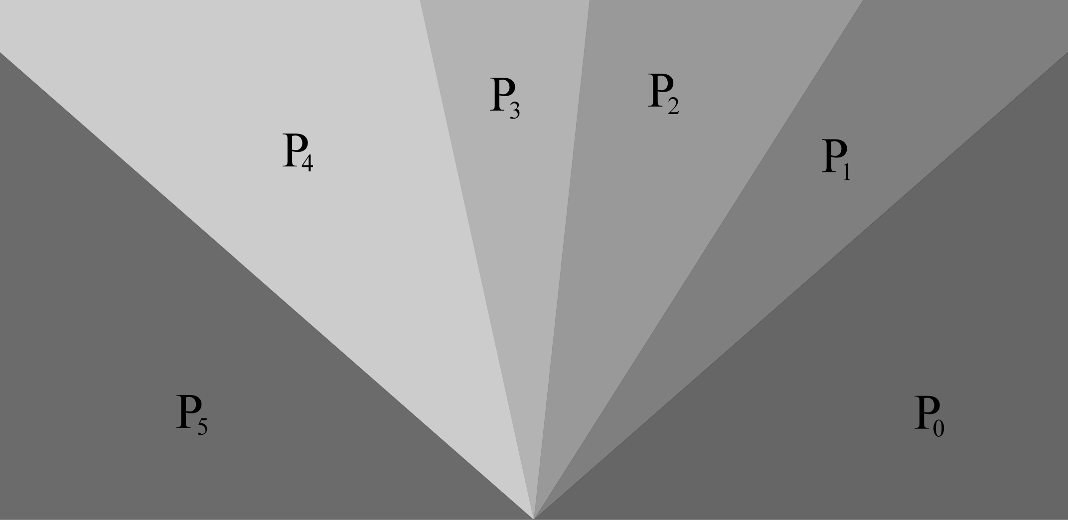
Figure 1. An example of a partition of the closed upper half plane $\overline{\mathbb{H}}$ into 6 cones.

Let $\operatorname{Sym}(d)$ denote the group of permutations on the set $\{1,...,d\}$, $\tau\in\operatorname{Sym}(d)$, and let

(2.2) $$\theta_{j}(\alpha,\tau)=\sum_{\tau(k)<\tau(j)}\alpha_{k}-\sum_{k<j}\alpha_{k}.$$

When $\alpha$ and $\tau$ are unambiguous, we may refer to $\theta_{j}(\alpha,\tau)$ simply as $\theta_{j}$. The map $E:\overline{\mathbb{H}}\rightarrow\overline{\mathbb{H}}$ is then defined as

$$E(z)=\begin{cases}z,&\text{ if }z\in P_{0}\cup P_{d+1},\\ ze^{i\theta_{j}},&\text{ if }z\in P_{j},j\in\{1,...,d\}.\end{cases}$$

Note that $E$ is invertible Lebesgue-almost everywhere in $\overline{\mathbb{H}}$. We define the middle cone $P_{c}$ of $F_{\kappa}$ as

$$P_{c}=\bigcup_{j=1}^{d}P_{j}=\mathbb{H}\setminus(P_{0}\cup P_{d+1}).$$

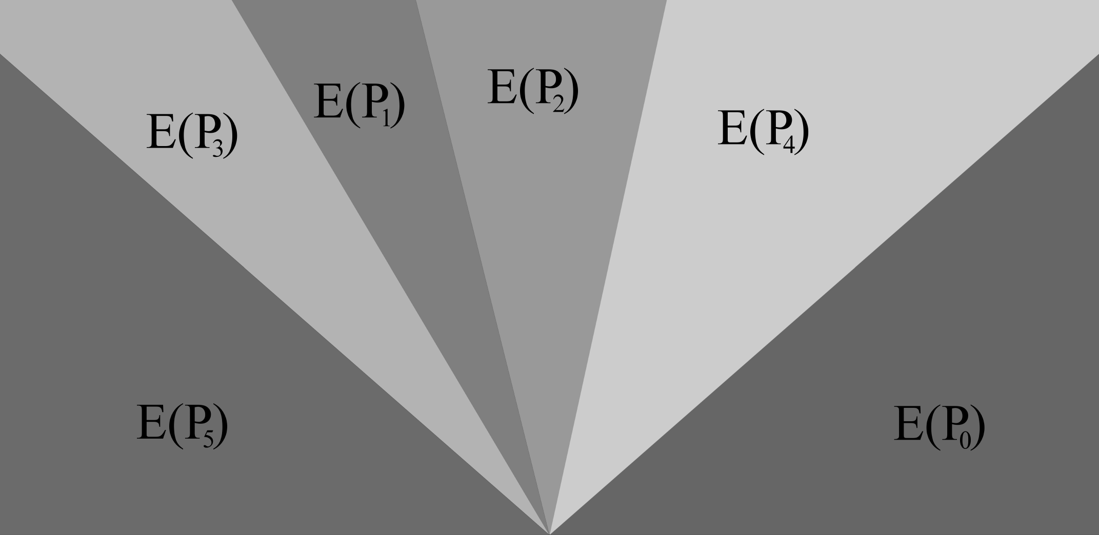
Figure 2. The partition from figure 1 after an application of some example cone exchange $E$.

The map $G:\overline{\mathbb{H}}\rightarrow\overline{\mathbb{H}}$ is defined as

$$G(z)=\begin{cases}z-\rho,&\text{ if }z\in P_{0},\\ z-\eta,&\text{ if }z\in P_{c},\\ z+\lambda,&\text{ if }z\in P_{d+1},\end{cases}$$

where $\rho,\lambda\in(0,\infty)$ are rationally independent and $0<\eta<\lambda$. Finally, we define the mapping $F_{\kappa}$ as the composition (as we have seen, $E$ is a permutation of the cones $P_{1},...,P_{d}$, and $G$ a piecewise horizontal translation)

$$F_{\kappa}(z)=G\circ E(z).$$

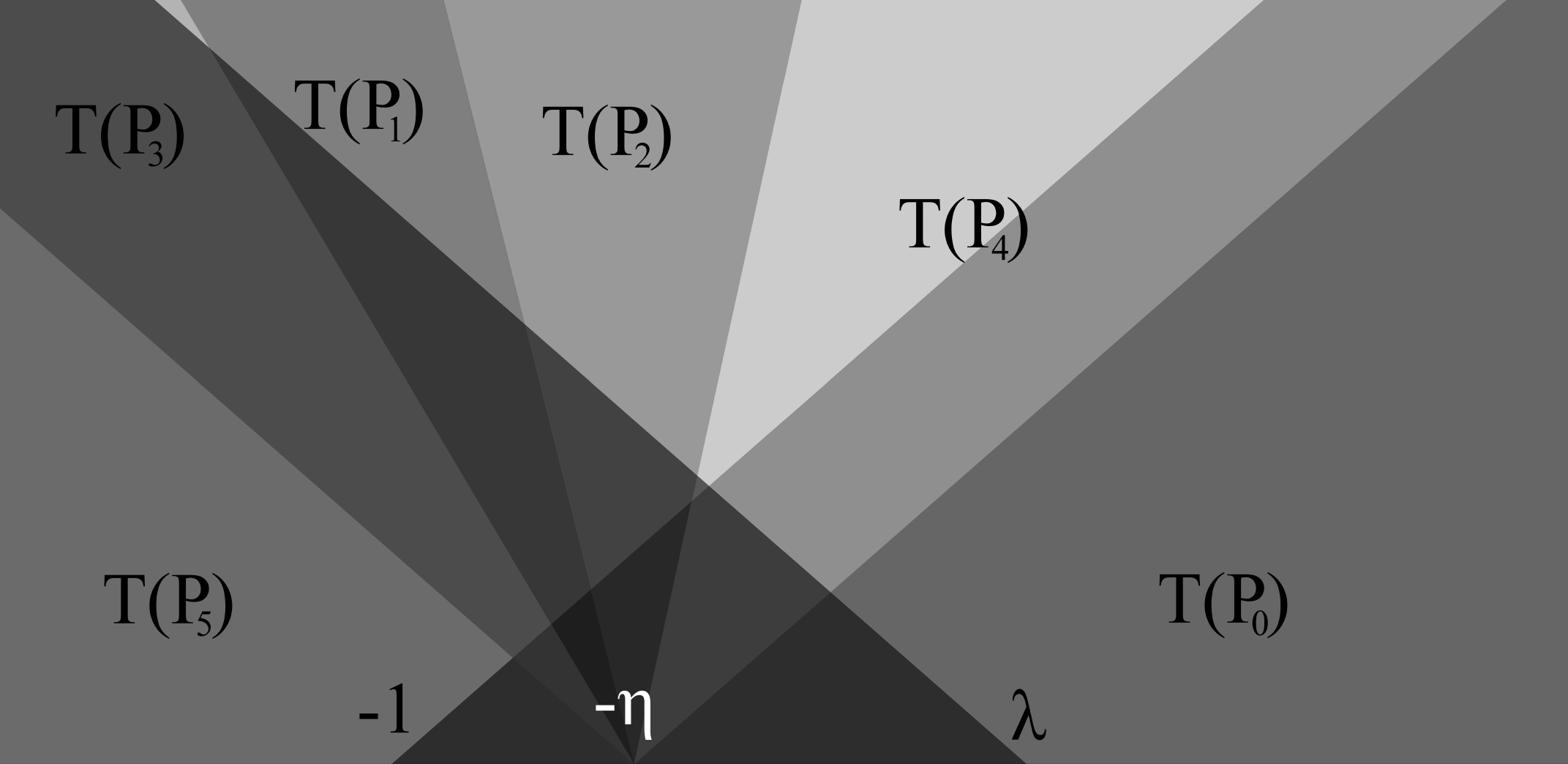
Figure 3. The exchanged partition from figure 2 after an application of an example piecewise translation $G$. Equivalently, the partition from figure 1 after an application of the TCE $F_{\kappa}$.

3. Main Results

Let $n\in\mathbb{N}\setminus\{0\}$ and suppose that

(3.1) $$\eta =\rho-\lambda>0,$$

$$\alpha =\left(\frac{\pi}{2}-\phi,\phi,\phi,\frac{\pi}{2}-\phi\right),$$

$$\tau =(2\hskip 4.30554pt1),\text{ and}$$

$$l^{(n)} =\lambda-2n\eta(1+\cos\phi)=(2n(1+\cos\phi)+1)\lambda-2n(1+\cos\phi)\rho\geq 0,$$

for some $0<\phi<\frac{\pi}{2}$, where the permutation $\tau\in\operatorname{Sym}(2)$ is written in cycle notation.

We define a finite sequence of points $(a_{k}^{(n)})_{k=0}^{4n+3}$ by

(3.2) $$a_{0}^{(n)} =n\eta(1+\cos\phi)-\rho+in\eta\frac{1+\cos\phi}{\tan\phi},$$

$$a_{1}^{(n)} =a_{0}^{(n)}+l^{(n)}=-\eta-n\eta(1+\cos\phi)+in\eta\frac{1+\cos\phi}{\tan\phi},$$

$$a_{k+1}^{(n)} =\begin{cases}a_{k}^{(n)}+\eta&\text{ if $k$ is odd,}\\ a_{k}^{(n)}+\eta e^{i\phi}&\text{ if $k$ is even, }1<k\leq 2n+1,\\ a_{k}^{(n)}+\eta e^{-i\phi}&\text{ if $k$ is even, }2n+1<k\leq 4n+2,\end{cases}$$

$$a_{4n+3}^{(n)} =a_{4n+2}^{(n)}+l^{(n)}.$$

This sequence defines the vertices for a piecewise linear curve $\gamma^{(n)}:I\rightarrow\overline{\mathbb{H}}$ we shall call an $n$-stepped cap. Let $Y^{(n)}$ denote the polygonal region bounded by the curves,

$$\gamma^{(n)}(I),$$

$$\{(1-t)(-\rho)+ta_{0}^{(n)}:t\in[0,1]\},$$

$$[-\rho,\lambda],\text{ and}$$

$$\{(1-t)\lambda+ta_{7}^{(n)}:t\in[0,1]\}.$$

We call $Y^{(n)}$ an $n$-stepped pyramid. See figures 5 and 6.

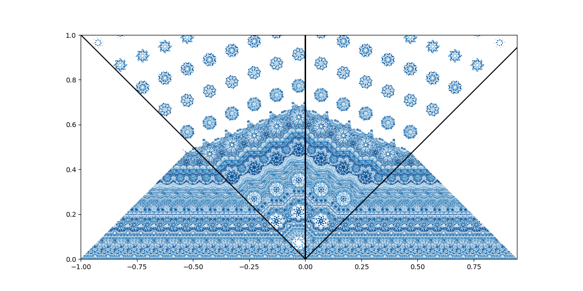
Figure 4. A similar plot as figure 7 within the box $[-1,\lambda]\times[0,1]$, but with parameters $\phi=\pi/4$, $\lambda=\frac{8+4\sqrt{2}}{9+4\sqrt{2}}+0.01$ and $\rho=1$. Note the appearance of more curves with an increasing number of steps.

Theorem 3.1.

Let $n\in\mathbb{N}\setminus\{0\}$, let $\eta>0$, $\alpha$, $\tau$ and $l^{(n)}\geq 0$ be as in (3.1), $(a_{k}^{(n)})_{k=0}^{4n+3}$ as in (3.2), and let $\gamma^{(n)}$ and $Y^{(n)}$ be the $n$-stepped cap and pyramid given by $(a_{k}^{(n)})_{k}$. Then $\gamma^{(n)}(I)$ and $Y^{(n)}$ are $F_{\kappa}$-invariant, up to measure zero. Moreover, $\gamma^{(n)}$ is an embedding of an IET into $(\mathcal{P},F_{\kappa})$.

Proof.

Observe that

(3.3) $$a_{2}^{(n)} =a_{1}^{(n)}+\eta$$

$$=-n\eta(1+\cos\phi)+in\eta\frac{1+\cos\phi}{\tan\phi}$$

$$=n\eta\frac{1+\cos\phi}{\sin\phi}(-\sin\phi+i\cos\phi)$$

$$=n\eta\frac{1+\cos\phi}{\sin\phi}e^{i\left(\phi+\frac{\pi}{2}\right)}\in\overline{P_{2}}\cap\overline{P_{3}}.$$

Secondly, noting that

$$\sin\phi+\frac{1+\cos\phi}{\tan\phi}=\frac{1}{\sin\phi}((\sin\phi)^{2}+\cos\phi+(\cos\phi)^{2})=\frac{1+\cos\phi}{\sin\phi},$$

we have

(3.4) $$a_{2n+2}^{(n)} =a_{2}^{(n)}+\sum_{j=1}^{n}\eta+\sum_{j=1}^{n}\eta e^{i\phi}$$

$$=-n\eta(1+\cos\phi)+in\eta\frac{1+\cos\phi}{\tan\phi}+n\eta+n\eta e^{i\phi},$$

$$=in\eta\left(\sin\phi+\frac{1+\cos\phi}{\tan\phi}\right)$$

$$=in\eta\frac{1+\cos\phi}{\sin\phi}\in\overline{P_{1}}\cap\overline{P_{2}}.$$

Thirdly, we have

(3.5) $$a_{4n+2}^{(n)} =a_{2n+2}^{(n)}+\sum_{j=1}^{n}\eta+\sum_{j=1}^{n}\eta e^{-i\phi}$$

$$=in\eta\left(\sin\phi+\frac{1+\cos\phi}{\tan\phi}\right)+n\eta+n\eta e^{-i\phi},$$

$$=in\eta\sin\phi+in\eta\frac{1+\cos\phi}{\tan\phi}+n\eta+n\eta\cos\phi-in\eta\sin\phi$$

$$=n\eta\frac{1+\cos\phi}{\sin\phi}\left(\sin\phi+i\cos\phi\right)$$

$$=n\eta\frac{1+\cos\phi}{\sin\phi}e^{i\left(\frac{\pi}{2}-\phi\right)}\in\overline{P_{0}}\cap\overline{P_{1}}.$$

We can thus partition the set $\gamma^{(n)}(I)$ into four segments, excluding their endpoints,

(3.6) $$\gamma_{0}^{(n)} \subset P_{3}\text{ from $a_{0}^{(n)}$ to $a_{2}^{(n)}$,}$$

$$\gamma_{1}^{(n)} \subset P_{2}\text{ from $a_{2}^{(n)}$ to $a_{2n+2}^{(n)}$,}$$

$$\gamma_{2}^{(n)} \subset P_{1}\text{ from $a_{2n+2}^{(n)}$ to $a_{4n+2}^{(n)}$, and}$$

$$\gamma_{3}^{(n)} \subset P_{0}\text{ from $a_{4n+2}^{(n)}$ to $a_{4n+3}^{(n)}$.}$$

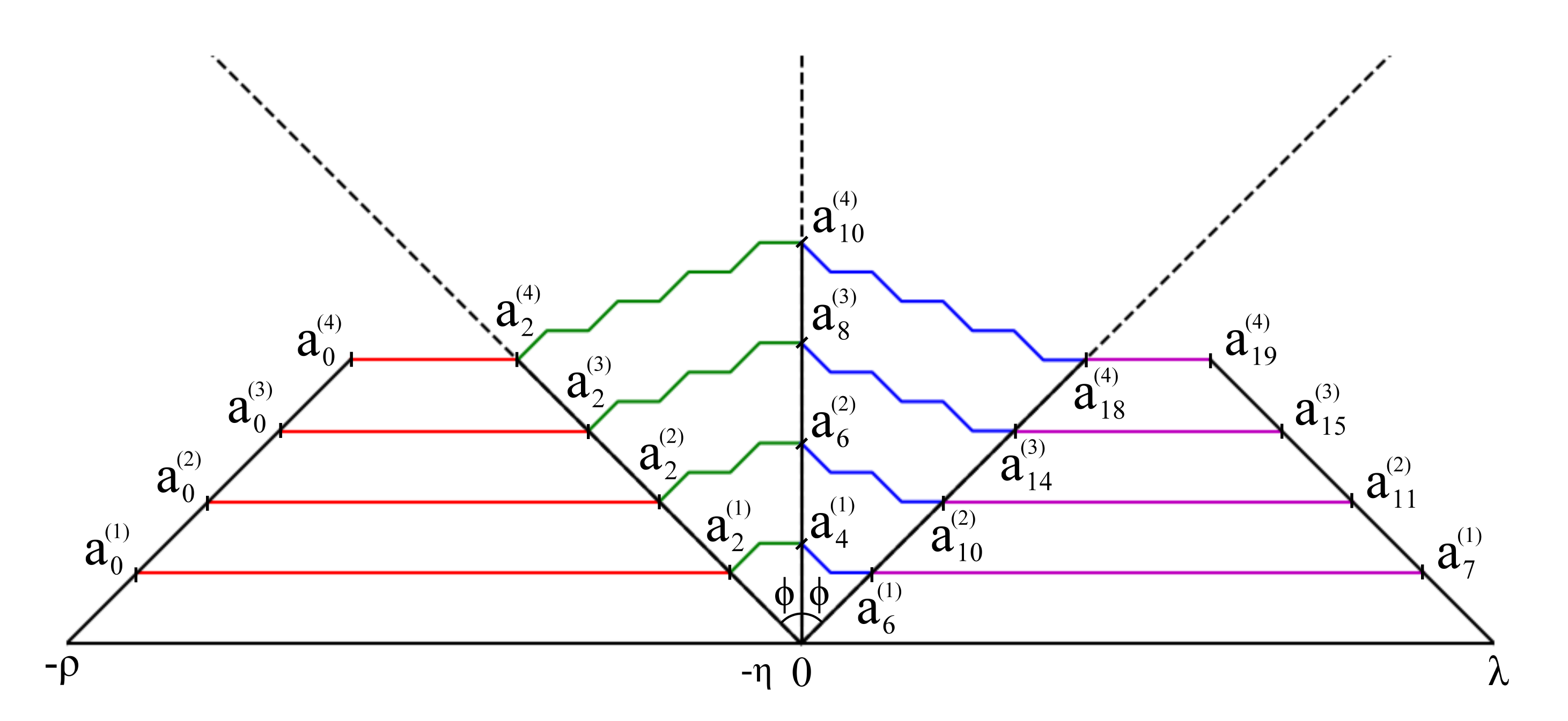
Figure 5. An illustration of $n$-stepped caps for $n=1,2,3,4$ ascending from the bottom curve, with the same parameters as in figure 4, which each form the “cap” of the boundary for their respective $n$-stepped pyramid. The curves $\gamma^{(n)}$ have been coloured into the segments $\gamma_{k}^{(n)}$ from (3.6), i.e. $\gamma^{(n)}$ is partitioned according to which cone the segment belongs to.

Let us also partition the set $\gamma^{(n)}(I)$ into

(3.7) $$\gamma_{0}^{(n)^{\prime}}\text{ from $a_{0}^{(n)}$ to $a_{1}^{(n)}$,}$$

$$\gamma_{1}^{(n)^{\prime}}\text{ from $a_{1}^{(n)}$ to $a_{2n+1}^{(n)}$,}$$

$$\gamma_{2}^{(n)^{\prime}}\text{ from $a_{2n+1}^{(n)}$ to $a_{4n+1}^{(n)}$, and}$$

$$\gamma_{3}^{(n)^{\prime}}\text{ from $a_{4n+1}^{(n)}$ to $a_{4n+3}^{(n)}$.}$$

To prove the $F_{\kappa}$-invariance of $\gamma^{(n)}$, it suffices to show that

(3.8) $$F_{\kappa}(\gamma_{j}^{(n)})=\gamma_{3-j}^{(n)^{\prime}},$$

for $j=0,1,2,3$.

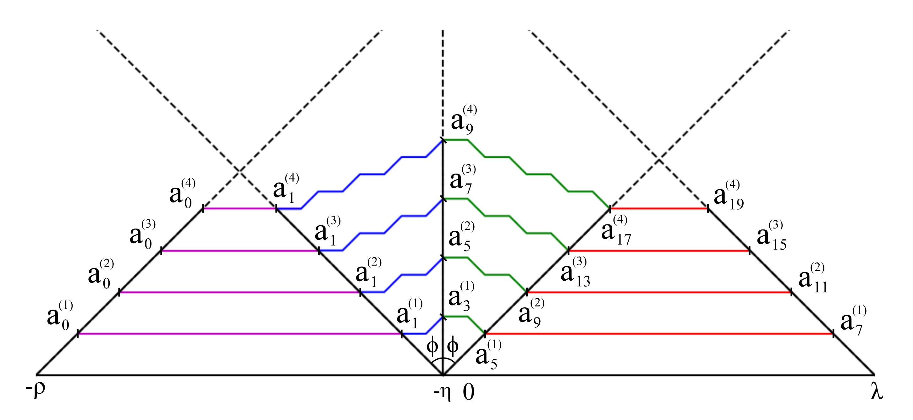
Figure 6. The $n$-stepped caps as in figure 5, but mapped under the TCE $T$ with the same parameters. Observe that the curves seem to overall be preserved, although the individually coloured pieces are rearranged within each curve into the partition $\gamma_{k}^{(n)^{\prime}}$ as in (3.7), which is akin to an interval exchange transformation. Additionally note that the $n$-stepped pyramids also appear to be preserved under $T$.

Observe that by (3.5),

$$a_{0}^{(n)} =n\eta(1+\cos\phi)-\rho+in\eta\frac{1+\cos\phi}{\tan\phi}$$

$$=n\eta\frac{1+\cos\phi}{\sin\phi}\left(\sin\phi+i\cos\phi\right)-\rho$$

$$=a_{4n+2}^{(n)}-\rho.$$

Hence,

$$a_{1}^{(n)}=a_{0}^{(n)}+l^{(n)}=a_{4n+2}^{(n)}-\rho+l^{(n)}=a_{4n+3}^{(n)}-\rho,$$

so by (3.6) we have

$$F_{\kappa}(\gamma_{3}^{(n)})=\gamma_{3}^{(n)}-\rho=\gamma_{0}^{(n)^{\prime}}.$$

Similarly, we have

$$a_{4n+1}^{(n)}=a_{4n+2}^{(n)}-\eta=a_{4n+2}-\rho+\lambda=a_{0}^{(n)}+\lambda,$$

from which we deduce

$$a_{4n+3}^{(n)}=a_{4n+1}^{(n)}+\eta+l^{(n)}=a_{0}^{(n)}+\lambda+\eta+l^{(n)}=a_{2}^{(n)}+\lambda,$$

and thus by (3.6), we get

$$F_{\kappa}(\gamma_{0}^{(n)})=\gamma_{0}^{(n)}+\lambda=\gamma_{3}^{(n)^{\prime}}.$$

We know that

$$F_{\kappa}(\gamma_{1}^{(n)})=e^{-i\phi}\gamma_{1}^{(n)}-\eta,$$

since $\gamma_{1}^{(n)}\subset P_{2}$. Recall from (3.2) that for $2<k\leq 2n+2$

$$a_{k}^{(n)}=\begin{cases}a_{k-1}^{(n)}+\eta&\text{ if $k-1$ is odd},\\ a_{k-1}^{(n)}+\eta e^{i\phi}&\text{ if $k-1$ is even}.\end{cases}$$

From this, it follows from distributing and rearranging terms that

(3.9) $$e^{-i\phi}a_{k}^{(n)}-\eta =\begin{cases}e^{-i\phi}(a_{k-1}^{(n)}+\eta)-\eta&\text{ if $k-1$ is odd},\\ e^{-i\phi}(a_{k-1}^{(n)}+\eta e^{i\phi})-\eta&\text{ if $k-1$ is even},\end{cases}$$

$$=\begin{cases}(e^{-i\phi}a_{k-1}^{(n)}-\eta)+\eta e^{-i\phi}&\text{ if $k-1$ is odd},\\ (e^{-i\phi}a_{k-1}^{(n)}-\eta)+\eta&\text{ if $k-1$ is even}.\end{cases}$$

In addition, we can see from comparison of (3.3) and (3.4)

(3.10) $$a_{2n+2}^{(n)}=e^{-i\phi}a_{2}^{(n)}.$$

By using (3.2) in the case $k=2n+1$, we see that

(3.11) $$a_{2n+1}^{(n)}=a_{2n+2}^{(n)}-\eta=e^{-i\phi}a_{2}^{(n)}-\eta.$$

Using (3.11) and (3.9), we can use an inductive argument to show that for $2\leq k\leq 2n+2$,

(3.12) $$e^{-i\phi}a_{k}^{(n)}-\eta=a_{2n+k-1}^{(n)},$$

from which it follows from inspection of the definition of $\gamma_{2}^{(n)^{\prime}}$ in (3.7) that

$$F_{\kappa}(\gamma_{1}^{(n)})=e^{-i\phi}\gamma_{1}^{(n)}-\eta=\gamma_{2}^{(n)^{\prime}}.$$

In a similar fashion, recall from (3.6) that $\gamma_{2}^{(n)}\subset P_{1}$, so

$$F_{\kappa}(\gamma_{2}^{(n)})=e^{i\phi}\gamma_{2}^{(n)}-\eta.$$

Recall from (3.2) that for $2n+2<k\leq 4n+2$ that

$$a_{k}^{(n)}=\begin{cases}a_{k-1}^{(n)}+\eta&\text{ if $k-1$ is odd},\\ a_{k-1}^{(n)}+\eta e^{-i\phi}&\text{ if $k-1$ is even}.\end{cases}$$

We thus have

(3.13) $$e^{i\phi}a_{k}^{(n)}-\eta =\begin{cases}e^{i\phi}(a_{k-1}^{(n)}+\eta)-\eta&\text{ if $k-1$ is odd},\\ e^{i\phi}(a_{k-1}^{(n)}+\eta e^{-i\phi})-\eta&\text{ if $k-1$ is even},\end{cases}$$

$$=\begin{cases}(e^{i\phi}a_{k-1}^{(n)}-\eta)+\eta e^{i\phi}&\text{ if $k-1$ is odd},\\ (e^{i\phi}a_{k-1}^{(n)}-\eta)+\eta&\text{ if $k-1$ is even}.\end{cases}$$

Recalling (3.10), and using (3.2) in the case $k=1$ we see that

(3.14) $$a_{1}^{(n)}=a_{2}^{(n)}-\eta=e^{i\phi}a_{2n+2}^{(n)}-\eta.$$

Recalling the definition of $\gamma_{1}^{(n)^{\prime}}$ in (3.7), then combining (3.14) and (3.13), we can use another inductive argument to show that for $2n+2\leq k\leq 4n+2$,

(3.15) $$e^{i\phi}a_{k}^{(n)}-\eta=a_{k-2n-1}^{(n)}.$$

Hence, it follows from the definition of $\gamma_{1}^{(n)^{\prime}}$ in (3.7) that

$$F_{\kappa}(\gamma_{2}^{(n)})=e^{i\phi}\gamma_{2}^{(n)}-\eta=\gamma_{1}^{(n)^{\prime}}.$$

We have thus proven (3.8), from which it follows that

$$F_{\kappa}(\gamma^{(n)}(I)) =F_{\kappa}(\gamma_{0}^{(n)})\cup F_{\kappa}(\gamma_{1}^{(n)})\cup F_{\kappa}(\gamma_{2}^{(n)})\cup F_{\kappa}(\gamma_{3}^{(n)}),$$

$$=\gamma_{3}^{(n)^{\prime}}\cup\gamma_{2}^{(n)^{\prime}}\cup\gamma_{1}^{(n)^{\prime}}\cup\gamma_{0}^{(n)^{\prime}}$$

$$=\gamma^{(n)}(I),$$

up to a set of 0 one-dimensional Lebesgue measure.

It is clear from the exchange of the segments $\gamma_{0}^{(n)}$, $\gamma_{1}^{(n)}$, $\gamma_{2}^{(n)}$, $\gamma_{3}^{(n)}$ as well as their lengths that the mapping $T|_{\gamma(I)}$ is conjugate to an IET with combinatorial data

(3.16) $$\sigma^{(n)} =\begin{pmatrix}A&B&C&D\\ D&C&B&A\end{pmatrix},$$

$$\xi^{(n)} =(l^{(n)}+\eta,2n\eta,2n\eta,l^{(n)}).$$

Note that the superscript $n$ here is not to be confused with Rauzy induction. To prove that $Y^{(n)}$ is $F_{\kappa}$-invariant, it suffices to show that each atom in $\mathcal{Q}^{(n)}=\mathcal{P}\vee Y^{(n)}=\{P\cap Y^{(n)}:P\in\mathcal{P}\}$ intersects the others at most on its boundary, that their image under $F_{\kappa}$ is contained in $Y^{(n)}$. For brevity, from now on we will denote the open polygon with vertices $x_{0}$,…,$x_{N-1}$ and edges $(x_{k},x_{k+1})$ and $(x_{N-1},x_{0})$ by $[x_{0},...,x_{N-1}]$. Note that if $S:\mathbb{C}\rightarrow\mathbb{C}$ is any isometry on $\mathbb{C}$, then

$$S([x_{0},...,x_{N-1}])=[S(x_{0}),...,S(x_{N-1})].$$

For $j=0,1,2,3$, let

(3.17) $$Q_{j}^{(n)}=Y^{(n)}\cap P_{j}.$$

By the definition of $Y^{(n)}$ in (3) and the properties (3.3), (3.4) and (3.5) of the points $a_{2}^{(n)}$, $a_{2n}^{(n)}$ and $a_{4n+2}^{(n)}$ respectively, we have

$$Q_{0}^{(n)} =[0,a_{4n+2}^{(n)},a_{4n+3}^{(n)},\lambda],$$

$$Q_{1}^{(n)} =[0,a_{2n+2}^{(n)},a_{2n+3}^{(n)},...,a_{4n+2}^{(n)}],$$

$$Q_{2}^{(n)} =[0,a_{2}^{(n)},a_{3}^{(n)},...,a_{2n+2}^{(n)}],$$

$$Q_{3}^{(n)} =[-\rho,a_{0}^{(n)},a_{2}^{(n)},0].$$

Since $Q_{j}\subset P_{j}$ for each $j=0,1,2,3$, we have

(3.18) $$F_{\kappa}(Q_{0}^{(n)}) =[0,a_{4n+2}^{(n)},a_{4n+3}^{(n)},\lambda]-\rho=[-\rho,a_{0}^{(n)},a_{1}^{(n)},-\eta],$$

$$F_{\kappa}(Q_{3}^{(n)}) =[-\rho,a_{0}^{(n)},a_{2}^{(n)},0]+\lambda=[-\eta,a_{4n+1}^{(n)},a_{4n+3}^{(n)},\lambda].$$

Recall (3.12), then it is clear to see that

(3.19) $$F_{\kappa}(Q_{1}^{(n)}) =e^{i\phi}[0,a_{2n+2}^{(n)},...,a_{4n+2}^{(n)}]-\eta$$

$$=[-\eta,e^{i\phi}a_{2n+2}^{(n)}-\eta,...,e^{i\phi}a_{4n+2}^{(n)}-\eta]$$

$$=[-\eta,a_{1}^{(n)},...,a_{2n+1}^{(n)}].$$

Similarly by recalling (3.15) we get

(3.20) $$F_{\kappa}(Q_{2}^{(n)}) =e^{-i\phi}[0,a_{2}^{(n)},...,a_{2n+2}^{(n)}]-\eta$$

$$=[-\eta,e^{-i\phi}a_{2}^{(n)}-\eta,...,e^{-i\phi}a_{2n+2}^{(n)}-\eta]$$

$$=[-\eta,a_{2n+1}^{(n)},...,a_{4n+1}^{(n)}].$$

It is clear from (3.18), (3.19), (3.20) that $F_{\kappa}(Y^{(n)})\subset Y^{(n)}$, and the only nonempty intersections are

$$\overline{F_{\kappa}(Q_{0}^{(n)})}\cap\overline{F_{\kappa}(Q_{1}^{(n)})} =\{-\eta t+(1-t)a_{1}^{(n)}:t\in[0,1]\},$$

$$\overline{F_{\kappa}(Q_{1}^{(n)})}\cap\overline{F_{\kappa}(Q_{2}^{(n)})} =\{-\eta t+(1-t)a_{2n+1}^{(n)}:t\in[0,1]\},$$

$$\overline{F_{\kappa}(Q_{2}^{(n)})}\cap\overline{F_{\kappa}(Q_{3}^{(n)})} =\{-\eta t+(1-t)a_{4n+1}^{(n)}:t\in[0,1]\},$$

and $\overline{F_{\kappa}(Q_{0}^{(n)})}\cap\overline{F_{\kappa}(Q_{1}^{(n)})}\cap\overline{F_{\kappa}(Q_{2}^{(n)})}\cap\overline{F_{\kappa}(Q_{3}^{(n)})}=\{-\eta\}$. All of these intersections are on the boundaries of the atoms, and thus have 0 two-dimensional Lebesgue measure. Therefore $Y^{(n)}$ is $F_{\kappa}$-invariant up to zero measure. ∎

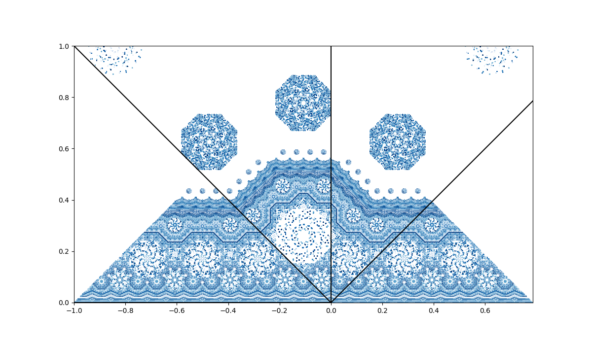
Figure 7. A plot of 1000 iterates in the orbits of 500 uniformly distributed points in the box $[-1,\lambda]\times[0,1]$ under the TCE with parameters as in (3.1), where $\phi=\pi/4$, $\lambda=\pi/4$ and $\rho=1$. Note the appearance of a piecewise linear curve near the top of the maximal invariant set.

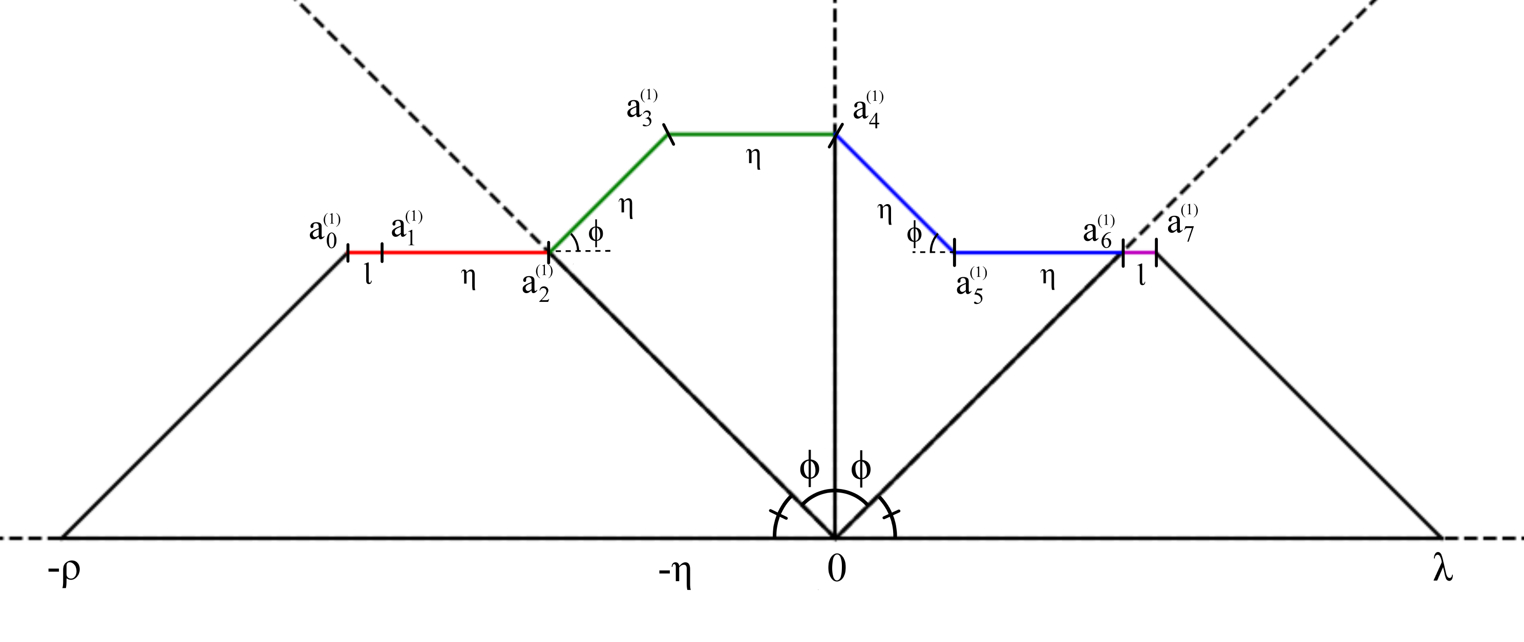
Figure 8. A more detailed illustration of the one-stepped curve $\gamma^{(1)}$ from the example TCE in 7, as well as the one-stepped pyramid $Y^{(1)}$ below it. Observe that the restriction of the TCE $(\mathcal{P},F_{\kappa})$ to the region $Y^{(1)}$ is a PWI with a non-convex atom.

Remark 3.2.

Observe that

$$l^{(n)}=\lambda-2n\eta(1+\cos\phi)<\lambda-2(n-1)\eta(1+\cos\phi)=l^{(n-1)},$$

In other words, $l^{(n)}\geq 0$ implies that $l^{(k)}\geq 0$ for all $1\leq k\leq n$. Hence, if $l^{(n)}\geq 0$, then for all $1\leq k\leq n$, the curve $\gamma^{(k)}$ is an invariant curve for the TCE $(\mathcal{P},F_{\kappa})$.

Corollary 3.3 (Invariant Layers).

Let $n>1$ be an integer, and let $\eta>0$, $\alpha$, $\tau$ and $l^{(n)}\geq 0$ be as in (3.1), $(a_{k}^{(n)})_{k=0}^{4n+3}$ as in (3.2), and let $\gamma^{(n)}$ and $Y^{(n)}$ be the $n$-stepped cap and pyramid given by $(a_{k}^{(n)})_{k}$. Then $Y^{(k)}\setminus Y^{(k-1)}$ is an invariant region for all $1<k\leq n$.

Proof.

It suffices to prove that $Y^{(n)}\setminus Y^{(n-1)}$ is $F_{\kappa}$-invariant, since by Remark 3.2 we can apply the same argument to $Y^{(k)}\setminus Y^{(k-1)}$ for all $k<n$. Recall that by Theorem 3.1, $Y^{(n)}$ and $Y^{(n-1)}$ are $T$-invariant. Thus, $F_{\kappa}|_{Y^{(n)}}$ and $F_{\kappa}|_{Y^{(n-1)}}$ are invertible, and we have that

$$Y^{(n-1)}=F_{\kappa}|_{Y^{(n)}}^{-1}(Y^{(n-1)}).$$

Therefore,

$$\left(Y^{(n)}\setminus Y^{(n-1)}\right)\cap F_{\kappa}|_{Y^{(n)}}^{-1}(Y^{(n-1)})=\emptyset.$$

By the invariance of $Y^{(n)}$, this implies

$$Y^{(n)}\setminus Y^{(n-1)}\subseteq F_{\kappa}|_{Y^{(n)}}^{-1}(Y^{(n)}\setminus Y^{(n-1)}),$$

but $F_{\kappa}|_{Y^{(n)}}$ is area-preserving since it is invertible, so in fact

$$Y^{(n)}\setminus Y^{(n-1)}=F_{\kappa}|_{Y^{(n)}}^{-1}(Y^{(n)}\setminus Y^{(n-1)}).$$

∎

Remark 3.4.

The conditions that $l^{(n)}\geq 0$ and $\lambda\leq\rho$ are equivalent to the inequality

(3.21) $$\frac{2n(1+\cos\phi)}{2n(1+\cos\phi)+1}\rho\leq\lambda\leq\rho,$$

and if we divide by $\rho$, this is in turn equivalent to

$$1-\frac{1}{2n(1+\cos\phi)+1}\leq\frac{\lambda}{\rho}\leq 1.$$

This confirms that as $\lambda\nearrow\rho$, $l^{(n)}\geq 0$ for arbitrarily large $n\in\mathbb{N}\setminus\{0\}$. On the other hand, if we subtract $\rho$ from all sides of the inequality (3.21), we get

$$\frac{2n(1+\cos\phi)}{2n(1+\cos\phi)+1}\rho-\rho\leq\lambda-\rho\leq 0,$$

which, by expanding the left hand side and recalling $\eta=\rho-\lambda$, gives us

$$0\leq\eta\leq\frac{\rho}{2n(1+\cos\phi)+1}.$$

This allows us to deduce a bound on the lengths of the middle segments $\gamma_{1}^{(n)}$ and $\gamma_{2}^{(n)}$ by multiplying by $2n$, that is

$$0\leq 2n\eta\leq\frac{\rho}{1+\cos\phi+\frac{1}{2n}}.$$

3.1. Reflective symmetry

So far, one restriction on the parameters has been that $\lambda\leq\rho$. As we will show now, this constraint can be relaxed by considering the reflective symmetry of the partition in the imaginary axis. Define $\mathcal{R}:\overline{\mathbb{H}}\rightarrow\overline{\mathbb{H}}$ by

(3.22) $$\mathcal{R}(z)=\mathcal{R}(x+iy)=-x+iy=-\overline{z},$$

that is, the reflection of $z=x+iy$ about the imaginary axis, where $x,y\in\mathbb{R}$, $y\geq 0$. Note that $\mathcal{R}$ is an involution, i.e. $\mathcal{R}^{-1}=\mathcal{R}$. Furthermore, $\mathcal{R}$ is clearly additive. Define $\tilde{\alpha}$ as the reverse of $\alpha$, i.e.

(3.23) $$\tilde{\alpha}=(\alpha_{d+1},...,\alpha_{0}),$$

then $\tilde{\tilde{\alpha}}=\alpha$ for all $\alpha\in\mathbb{B}^{d+2}$. Let $\tilde{\tau}$ denote the reverse of $\tau$ in the sense that

(3.24) $$\tilde{\tau}=\begin{pmatrix}\tilde{\tau}_{0}\\ \tilde{\tau}_{1}\end{pmatrix}=\begin{pmatrix}d&d-1&...&1\\ \tau(d)&\tau(d-1)&...&\tau(1)\end{pmatrix}.$$

Clearly, cone $\mathcal{R}(P_{j})$ has angle $\tilde{\alpha}_{j}=\alpha_{d+1-j}$.

Let $\mathcal{P}=\{P_{k}:k\in\{0,...,d+1\}\}$ denote the partition of $\overline{\mathbb{H}}$ into $d+2$ cones according to $\alpha$, and let $\tilde{\mathcal{P}}=\mathcal{R}(\mathcal{P})$ denote a similar partition of $\overline{\mathbb{H}}$ according into cones $\tilde{P}_{j}=\mathcal{R}(P_{d+1-j})$ of angle $\tilde{\alpha}_{j}=\alpha_{d+1-j}$. Set $F_{\tilde{\kappa}}$ to be the TCE with parameters $\tilde{\kappa}$, where

(3.25) $$\tilde{\kappa}=(\tilde{\alpha},\tilde{\tau},\rho,-\eta,\lambda).$$

Proposition 3.5.

We have the following conjugacy:

(3.26) $$F_{\tilde{\kappa}}(z)=\mathcal{R}\circ F_{\kappa}\circ\mathcal{R}(z).$$

Proof.

Observe that by (3.23) and (3.24), we get

$$\theta_{j}(\tilde{\alpha},\tilde{\tau}) =\sum_{\tilde{\tau}_{1}(k)<\tilde{\tau}_{1}(j)}\tilde{\alpha}_{k}-\sum_{\tilde{\tau}_{0}(k)<\tilde{\tau}_{0}(j)}\tilde{\alpha}_{k}$$

$$=\sum_{\tau(d+1-k)>\tau(d+1-j)}\alpha_{d+1-k}-\sum_{d+1-k>d+1-j}\alpha_{d+1-k}.$$

By relabelling $k$ to $d+1-k$, we get

$$\theta_{j}(\tilde{\alpha},\tilde{\tau})=\sum_{\tau(k)>\tau(d+1-j)}\alpha_{k}-\sum_{k>d+1-j}\alpha_{k}.$$

Recall that

$$\pi=\sum_{k=0}^{d+1}\alpha_{k}.$$

This implies that

$$\theta_{j}(\tilde{\alpha},\tilde{\tau}) =\left(\pi-\alpha_{0}-\alpha_{d+1}-\sum_{\tau(k)\leq\tau(d+1-j)}\alpha_{k}\right)-\left(\pi-\alpha_{0}-\alpha_{d+1}-\sum_{k\leq d+1-j}\alpha_{k}\right)$$

$$=-\left(\sum_{\tau(k)\leq\tau(d+1-j)}\alpha_{k}-\sum_{k\leq d+1-j}\alpha_{k}\right).$$

Note that since $\tau$ is a permutation of a finite set, $\tau(x)=\tau(y)$ if and only if $x=y$. Thus, we have

(3.27) $$\theta_{j}(\tilde{\alpha},\tilde{\tau})=-\left(\sum_{\tau(k)<\tau(d+1-j)}\alpha_{k}-\sum_{k<d+1-j}\alpha_{k}\right)=-\theta_{d+1-j}(\alpha,\tau).$$

Additionally, recall that for all $j\in\{0,...,d+1\}$,

$$\mathcal{R}(P_{j})=\tilde{P}_{d+1-j}.$$

Thus,

(3.28) $$\mathcal{R}(z)\in P_{j}\text{ if and only if }z\in\tilde{P}_{d+1-j}.$$

By expanding the definitions of $F_{\kappa}$ as in (2), we get

$$\mathcal{R}\circ F_{\kappa}\circ\mathcal{R}(z)=\begin{cases}\mathcal{R}(\mathcal{R}(z)+\lambda),&\text{ if }\mathcal{R}(z)\in P_{d+1},\\ \mathcal{R}(e^{i\theta_{j}(\alpha,\tau)}\mathcal{R}(z)-\eta),&\text{ if }\mathcal{R}(z)\in P_{j},j\in\{1,...,d\},\\ \mathcal{R}(\mathcal{R}(z)-\rho),&\text{ if }\mathcal{R}(z)\in P_{0}.\end{cases}$$

Using (3.28), and the definition of $\mathcal{R}$ as in (3.22), we get

$$\mathcal{R}\circ F_{\kappa}\circ\mathcal{R}(z)=\begin{cases}\mathcal{R}(-\overline{z}+\lambda),&\text{ if }z\in\tilde{P}_{d+1}\\ \mathcal{R}(-e^{i\theta_{j}(\alpha,\tau)}\overline{z}-\eta),&\text{ if }z\in\tilde{P}_{d+1-j},j\in\{1,...,d\},\\ \mathcal{R}(-\overline{z}-\rho),&\text{ if }z\in\tilde{P}_{0}.\end{cases}$$

Using the additivity of $\mathcal{R}$, as well as the fact that $\mathcal{R}(x)=-x$ when $x\in\mathbb{R}$, we have that

$$\mathcal{R}\circ F_{\kappa}\circ\mathcal{R}(z) =\begin{cases}\mathcal{R}(-\overline{z}+\lambda),&\text{ if }z\in\tilde{P}_{d+1},\\ \mathcal{R}(-e^{i\theta_{j}(\alpha,\tau)}\overline{z}-\eta),&\text{ if }z\in\tilde{P}_{d+1-j},j\in\{1,...,d\},\\ \mathcal{R}(-\overline{z}-\rho),&\text{ if }z\in\tilde{P}_{0},\end{cases}$$

$$=\begin{cases}z-\lambda,&\text{ if }z\in\tilde{P}_{d+1}\\ e^{-i\theta_{j}(\alpha,\tau)}z+\eta,&\text{ if }z\in\tilde{P}_{d+1-j},j\in\{1,...,d\}\\ z+\rho,&\text{ if }z\in\tilde{P}_{0}\end{cases}.$$

Observe that

$$\mathcal{R}\circ F_{\kappa}\circ\mathcal{R}(z)=e^{-i\theta_{j}}z+\eta\text{ when }z\in\tilde{P}_{d+1-j},$$

is equivalent to

$$\mathcal{R}\circ F_{\kappa}\circ\mathcal{R}(z)=e^{-i\theta_{d+1-j}}z+\eta\text{ when }z\in\tilde{P}_{j}.$$

Thus,

$$\mathcal{R}\circ F_{\kappa}\circ\mathcal{R}(z)=\begin{cases}z+\rho,&\text{ if }z\in\tilde{P}_{0},\\ e^{-i\theta_{d+1-j}(\alpha,\tau)}z+\eta,&\text{ if }z\in\tilde{P}_{j},j\in\{1,...,d\},\\ z-\lambda,&\text{ if }z\in\tilde{P}_{d+1}.\end{cases}$$

Finally, using (3.27) and comparing with the definition of $F_{\tilde{\kappa}}$ as in (3.25), this becomes

$$\mathcal{R}\circ F_{\kappa}\circ\mathcal{R}(z) =\begin{cases}z+\rho,&\text{ if }z\in\tilde{P}_{0},\\ e^{i\theta_{j}(\tilde{\alpha},\tilde{\tau})}z+\eta,&\text{ if }z\in\tilde{P}_{j},j\in\{1,...,d\},\\ z-\lambda,&\text{ if }z\in\tilde{P}_{d+1},\end{cases}$$

$$=F_{\tilde{\kappa}}(z).$$

∎

Recall in the context of this paper that $\alpha=(\pi/2-\phi,\phi,\phi,\pi/2-\phi)$ and $\tau=(2\hskip 4.30554pt1)$, both of which are palindromic. That is,

$$\tilde{\alpha} =\alpha,\text{ and }$$

$$\tilde{\tau} =\tau.$$

Therefore $\tilde{\mathcal{P}}=\mathcal{P}$, and crucially $\theta(\tilde{\alpha},\tilde{\tau})=\theta(\alpha,\tau)$. Thus, the only distinction between $F_{\kappa}$ and $F_{\tilde{\kappa}}$ in this case lies with the piecewise horizontal translations $G$ and $\tilde{G}$ for parameters $\kappa$, $\tilde{\kappa}$ respectively, i.e.

$$\tilde{G}(z)=\begin{cases}z+\lambda^{\prime},&\text{ if }z\in P_{d+1},\\ z-\eta^{\prime},&\text{ if }z\in P_{c},\\ z-\rho^{\prime},&\text{ if }z\in P_{0},\end{cases}$$

where $\lambda^{\prime}=\rho$, $\rho^{\prime}=\lambda$, and importantly

$$\eta^{\prime}=-\eta=\lambda-\rho=\rho^{\prime}-\lambda^{\prime}.$$

It can clearly be seen that the TCE $(\mathcal{P},F_{\tilde{\kappa}})$ also satisfies (3.1) except in that $\eta^{\prime}>0$ if and only if $\eta<0$. We can therefore deduce analogous results to those in Section 2 when $\eta<0$, by conjugating $(\mathcal{P},F_{\kappa})$ to a TCE $(\mathcal{P},F_{\tilde{\kappa}})$ in which $\eta>0$ and the results hold. Supposing that for each integer $n\geq 1$, the invariant curve and region for $(\mathcal{P},F_{\tilde{\kappa}})$ are $\gamma^{(n)}$ and $Y^{(n)}$ respectively, it is not too difficult to prove that the reflected curve $\mathcal{R}\circ\gamma^{(n)}$ and region $\mathcal{R}(Y^{(n)})$ are invariant for $(\mathcal{P},F_{\kappa})$.

3.2. Dynamics on the Invariant Curve

Let $I^{(n)}=\left[0,2l^{(n)}+(4n+1)\eta\right)$. Recall that for each integer $n>0$ for which (3.1) holds, there is an IET $(\mathcal{I}^{(n)},f_{\sigma^{(n)},\xi^{(n)}})$ defined by

(3.29) $$\mathcal{I}^{(n)} =\left.\begin{cases}I_{0}^{(n)}&=[0,l^{(n)}+\eta),\\ I_{1}^{(n)}&=[l^{(n)}+\eta,l^{(n)}+(2n+1)\eta),\\ I_{2}^{(n)}&=[l^{(n)}+(2n+1)\eta,l^{(n)}+(4n+1)\eta),\\ I_{3}^{(n)}&=[l^{(n)}+(4n+1)\eta,2l^{(n)}+(4n+1)\eta)\end{cases}\right\},$$

$$f_{\sigma^{(n)},\xi^{(n)}}(x) =\begin{cases}x+l^{(n)}+4n\eta&\text{ if }x\in I_{0}^{(n)},\\ x+(2n-1)\eta&\text{ if }x\in I_{1}^{(n)},\\ x-(2n+1)\eta&\text{ if }x\in I_{2}^{(n)},\\ x-l^{(n)}-(4n+1)\eta&\text{ if }x\in I_{3}^{(n)}.\\ \end{cases}$$

given by the combinatorial data $(\sigma^{(n)},\xi^{(n)})$ from (3.16). By Theorem 3.1, we have that for all $x\in I^{(n)}$,

$$F_{\kappa}\circ\gamma^{(n)}(x)=\gamma^{(n)}\circ f_{\sigma^{(n)},\xi^{(n)}}(x).$$

The first return map of $f_{\sigma^{(n)},\xi^{(n)}}$ to the first subinterval $I_{0}^{(n)}$ is a 2-IET with data

$$\xi^{(n)} =\begin{pmatrix}A&B\\ B&A\end{pmatrix},$$

$$\nu^{(n)} =\left(l^{(n)},\eta\right).$$

It is not so difficult to show that under $f_{\sigma^{(n)},\xi^{(n)}}$, the subinterval $I_{0}^{(n)}$ visits all of $I^{(n)}$ in $4n$ iterations, and that the dynamics of $f_{\sigma^{(n)},\xi^{(n)}}$ is determined by the first return map $f_{\xi^{(n)},\nu^{(n)}}$. In particular, orbits under $f_{\sigma^{(n)},\xi^{(n)}}$ are dense in $I^{(n)}$ if and only if they are dense in $I_{0}^{(n)}$ under $f_{\xi^{(n)},\nu^{(n)}}$. Due to the conjugation between 2-IETs and rotations of the circle, and assuming $\eta\neq 0$, orbits are dense on the curve if and only if

$$\frac{l^{(n)}}{\eta}\notin\mathbb{Q}.$$

Recalling that $l^{(n)}=\lambda-2n\eta(1+\cos\phi)$, this is equivalent to

$$\frac{\lambda}{\eta}\notin 2n\cos\phi+\mathbb{Q}.$$

Further recalling that $\eta=\rho-\lambda$, we have density of orbits on the curve if and only if

$$\frac{\lambda}{\rho}\neq\frac{p+2n(1+\cos\phi)q}{p+(1+2n(1+\cos\phi))q},$$

for all $p,q\in\mathbb{Z}$ with $q>0$.

Theorem 3.6.

For $x,y\in\mathbb{R}_{+}$, $x\neq y$, and $n\in\mathbb{N}\setminus\{0\}$, let

(3.30) $$\sigma^{(n)} =\begin{pmatrix}\sigma_{0}\\ \sigma_{1}\end{pmatrix}=\begin{pmatrix}A&B&C&D\\ D&C&B&A\end{pmatrix},\text{ and}$$

$$\nu^{(n)} =(x,2n|x-y|,2n|x-y|,y).$$

Then the IET given by the data $(\sigma^{(n)},\nu^{(n)})$ admits a piecewise linear, continuous embedding into some TCE.

Proof.

Let $x,y\in\mathbb{R}_{+}$ and suppose $x\neq y$, and set

(3.31) $$\lambda =2n(1+\cos\phi)x-(2n(1+\cos\phi)-1)y,\text{ and}$$

$$\rho =(2n(1+\cos\phi)+1)x-2n(1+\cos\phi)y,$$

Then we see that

$$\eta=\rho-\lambda=x-y.$$

Using the fact that $l^{(n)}=(2n(1+\cos\phi)+1)\lambda-2n(1+\cos\phi)\rho$ from (3.1), as well as (3.31), we get

$$l^{(n)} =(2n(1+\cos\phi)+1)\left(2n(1+\cos\phi)x-(2n(1+\cos\phi)-1)y\right)$$

$$-2n(1+\cos\phi)\left((2n(1+\cos\phi)+1)x-2n(1+\cos\phi)y\right)$$

$$=-(2n(1+\cos\phi)+1)(2n(1+\cos\phi)-1)y+2n(1+\cos\phi)^{2}y.$$

Letting $m=2n(1+\cos\phi)$ for visual clarity, this becomes

$$l^{(n)} =(m^{2}-(m-1)(m+1))y$$

$$=(m^{2}-(m^{2}-1))y$$

$$=y.$$

Therefore, we see that

$$l^{(n)}+\eta=x.$$

If $x>y$, then $\eta>0$ and by Theorem 3.1 the IET which embeds into $F_{\kappa}$ via $\gamma$ has data

$$\sigma^{(n)} =\begin{pmatrix}\sigma_{0}^{(n)}\\ \sigma_{1}^{(n)}\end{pmatrix}=\begin{pmatrix}A&B&C&D\\ D&C&B&A\end{pmatrix},\text{ and}$$

$$\nu^{(n)} =(x,2(x-y),2(x-y),y).$$

Now if $x<y$, then $\eta<0$, but the map $F_{\kappa}$ conjugates via a reflection in the imaginary axis to a TCE $F_{\tilde{\kappa}}$ by Proposition 3.5. In particular, we can interchange the placements of $x$ and $y$ in the previous statements to obtain the IET

$$\sigma^{(n)^{\prime}} =\begin{pmatrix}\sigma_{0}^{(n)^{\prime}}\\ \sigma_{1}^{(n)^{\prime}}\end{pmatrix}=\begin{pmatrix}A&B&C&D\\ D&C&B&A\end{pmatrix},\text{ and}$$

$$\nu^{(n)^{\prime}} =(y,2(y-x),2(y-x),x).$$

This IET embeds into the TCE $(\mathcal{P},F_{\tilde{\kappa}})$ via a curve $\gamma^{(n)^{\prime}}$, and thus the reflected IET

$$\sigma^{(n)} =\begin{pmatrix}\sigma_{0}^{(n)}\\ \sigma_{1}^{(n)}\end{pmatrix}=\begin{pmatrix}D&C&B&A\\ A&B&C&D\end{pmatrix},\text{ and}$$

$$\nu^{(n)} =(x,2(y-x),2(y-x),y),$$

embeds into the TCE $(\mathcal{P},F_{\kappa})$ via the reflected curve $\gamma^{(n)}=\mathcal{R}\circ\gamma^{(n)^{\prime}}$. Without loss of generality, we can relabel the letters in $\sigma^{(n)}$ so that $(\sigma^{(n)},\nu^{(n)})$ is of the form (3.30). ∎

Observe that the IET given by data $(\sigma^{(n)},\xi^{(n)})$ as in (3.16) does not satisfy the Keane condition. In particular, recall from (3.29) that

$$\partial I_{1}^{(n)}=l^{(n)}+\eta\text{ and }\partial I_{2}^{(n)}=l^{(n)}+(2n+1)\eta.$$

where $\partial[a,b)=a$. Then, by using the formula for $f_{\sigma^{(n)},\xi^{(n)}}$ in (3.29), a simple inductive argument shows that for $0\leq k\leq n-1$, we have

$$f^{2k+1}_{\sigma^{(n)},\xi^{(n)}}(l^{(n)}+\eta) =f^{2k}_{\sigma^{(n)},\xi^{(n)}}(l^{(n)}+2n\eta)$$

$$=l^{(n)}+(2n-2k)\eta.$$

Specifically, when $k=n-1$ we get

$$f^{2n-1}_{\sigma^{(n)},\xi^{(n)}}(l^{(n)}+\eta)=l^{(n)}+2\eta,$$

and finally,

$$f^{2n}_{\sigma^{(n)},\xi^{(n)}}(l^{(n)}+\eta)=l^{(n)}+2\eta+(2n-1)\eta=l^{(n)}+(2n+1)\eta=\partial I_{2}^{(n)}.$$

4. Discussion

The existence of a new concrete example of a family of TCEs that have invariant curves that are embeddings of IETs makes Theorem 3.1 the most important result of this paper, particularly as through Corollary 3.3 we conclude that these curves have the effect of restricting the distribution of orbits in the phase space. In particular, the invariance of $Y^{(n)}$ as in Theorem 3.1 and the invariance of the layers $Y^{(k)}\setminus Y^{(k-1)}$ as per Corollary 3.3 suggest that if the exceptional set intersects the interior of more than one layer, it cannot support an ergodic invariant measure. However, determining the set of parameters such that the exceptional set intersects in this way remains an open problem. Although the curves we study here are trivial embeddings in the sense of [8], they are nonetheless interesting in that they divide the phase space and they give information about nontrivial embeddings that may accumulate on them.

For such polygonal embeddings of IETs into PWIs, there is a connection between the renormalization structure of the IET and the geometry of its embedding, namely that the piecewise linear nature of some invariant curves could arise from a failure to meet the Keane condition, and that the number of pieces in a piecewise linear embedding roughly corresponds to the number of iterates it takes for two interval boundaries to coincide. This leads us to the hypothesis that when an IET-embedding does not consist of line segments or circle arcs, the underlying IET must satisfy the Keane condition.

Recall the PWI defined by $(\mathcal{Q}^{(n)},F_{\kappa}|_{Y^{(n)}})$, where $\mathcal{Q}^{(n)}$ is as in (3.17). Despite the appearance of non-convex atoms, we conjecture that the non-convex atom breaks down into convex cells after a finite number of dynamical refinements. This appears to be the case because the edges that produce this non-convexity are and remain on the boundary of $Y$ for all iterates. See figures 9 and 10 for example.

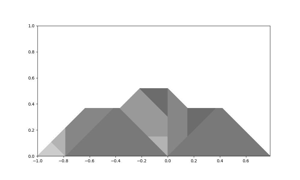
Figure 9. An illustration of the first dynamical refinement of the partition $\mathcal{Q}^{(1)}$ under the map $F_{\kappa}|_{Y^{(1)}}$, when $\lambda=\pi/4$ and $\phi=\pi/4$. Observe that the non-convex atom appears subdivided into convex pieces, meaning that the non-convexity is not pathological in this case, in that the encoding associated to each $n$-cell is unique.

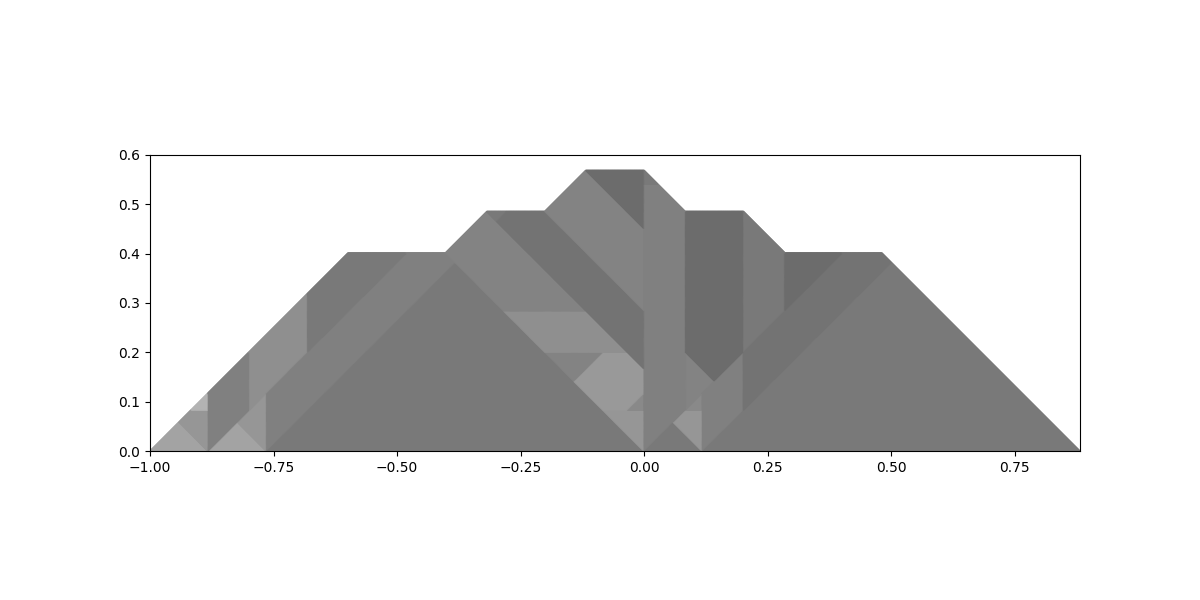
Figure 10. An illustration of the third dynamical refinement of the partition $\mathcal{Q}^{(2)}$ under the PWI $F_{\kappa}|_{Y^{(2)}}$ when $\lambda=\frac{4+2\sqrt{2}}{5+2\sqrt{2}}+0.01$ and $\phi=\pi/4$. Note that much like figure 9, the non-convex atoms in $\mathcal{Q}^{(2)}$ decompose into convex pieces under the refinement, although we need to reach a finer refinement to achieve this.

Consider the first return map $F_{\kappa}$ of $(\mathcal{Q}^{(n)},F_{\kappa}|_{Y^{(n)}})$ to the trapezium atom $Q_{3}^{(n)}=P_{3}\cap Y^{(n)}$. This mapping is a PWI, though the partition seems to depend on the angle, and in some cases it appears that the number of atoms is unbounded. In all cases, however, the mapping has the property its action on the top and bottom edges of $Q_{3}^{(n)}$ are two distinct 2-IETs. Thus the mapping on the trapezium $Q_{3}^{(n)}$ could perhaps be viewed as a transition map between these two IETs, though as of writing this map is unstudied. See figures 11 and 12. Especially note in figure 12 that when $l^{(n)}\geq 0$ for $n>1$, the trapezium $Q_{3}^{(n)}$ decomposes into three smaller invariant trapezia by corollary 3.3, and the map on each of these smaller trapezia appears to be similar to the first return map in the case that $n=1$. One question that arises is whether this PWI is uniquely defined by the 2-IETs on its edges. Specifically, given two 2-IETs $f_{1}$ and $f_{2}$ on intervals $I_{1}=[0,1)$ and $I_{2}=[1/2-a,1/2+a)$ for $0<a\leq 1/2$ and $h>0$, let $X$ denote the closed trapezium defined by the vertices $(0,0)$, $(1,0)$, $(1/2-a,h)$, and $(1/2+a,h)$. Let $\mathcal{T}_{f_{1},f_{2},h}$ denote the space of PWIs $(\mathcal{P},T)$ such that

$$T(x,0)=(f_{1}(x),0),\text{ for all }0\leq x<1,\\$$

and,

$$T(x,h)=(f_{2}(x),h),\text{ for all }1/2-a\leq x<1/2+a.$$

Then the questions become: What can we say about the space $\mathcal{T}_{f_{1},f_{2},h}$? What is its cardinality? If it contains more than one element, then what non-trivial connections can we draw between maps in this space?

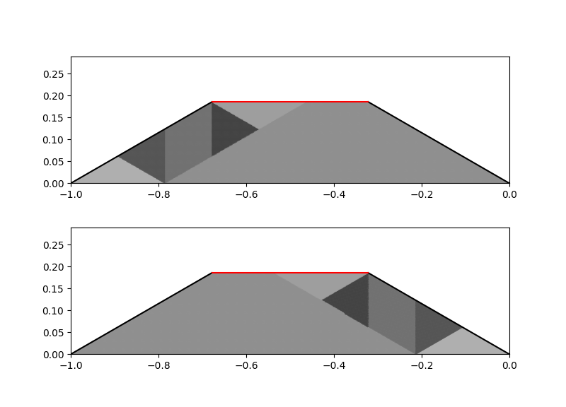
Figure 11. An illustration of the first return map of $(\mathcal{P},F_{\kappa})$ to the trapezium $Q_{3}^{(1)}$, with parameters in (3.1) where $\phi=\pi/4$, $\lambda=\pi/4$, and $\rho=1$.

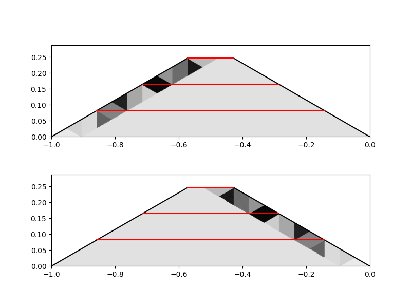
Figure 12. An illustration of the first return map of $(\mathcal{P},F_{\kappa})$ to the trapezium $Q_{3}^{(3)}$, with parameters in (3.1) where $\phi=\pi/4$, $\lambda=\frac{6+6\cos\phi}{7+6\cos\phi}+0.005$, and $\rho=1$.

References

- [1] Ashwin, P., (1997). Elliptic behaviour in the sawtooth standard map, Phys. Lett. A, 232, pp. 409-416.
- [2] Goetz, Arek, (2000). A self-similar example of a piecewise isometric attractor, Dynamical Systems: From Crystal to Chaos, 248-258.
- [3] Goetz, A. and Poggiaspalla, G., (2004). Rotations by /7, Nonlinearity, 17, no. 5, 1787.
- [4] Roy Adler, Bruce Kitchens, and Charles Tresser, (2001). Dynamics of non-ergodic piecewise affine maps of the torus, Ergodic Theory and Dynamical Systems, 21, no. 4, 959-999.
- [5] Lowenstein, John H., Konstantin L. Kouptsov, and Franco Vivaldi, (2003). Recursive tiling and geometry of piecewise rotations by /7, Nonlinearity, 17, no. 2, 371.
- [6] Ashwin, P. , Goetz, A. (2006). Polygonal invariant curves for a planar piecewise isometry. Trans. Amer. Math. Soc. 358 no. 1, 373-390.
- [7] Ashwin, P. , Goetz, A. (2005). Invariant curves and explosion of periodic islands in systems of piecewise rotations. SIAM J. Appl. Dyn. Syst., 4, no.2, 437-458.
- [8] Ashwin, P., Goetz, A., Peres, P. , Rodrigues, A. (2020). Embeddings of Interval Exchange Transformations in Planar Piecewise Isometries, Ergodic Theory and Dynamical Systems.
- [9] Kahng, Byungik, (2009). Singularities of two-dimensional invertible piecewise isometric dynamics, Chaos: An Interdisciplinary Journal of Nonlinear Science, 19, no. 2.
- [10] Boshernitzan, M.D., Carroll, (1997). An extension of Lagrange’s theorem to interval exchange transformations over quadratic fields. C.R. J. Anal. Math. 72: 21.
- [11] Buzzi, J. (2001). Piecewise isometries have zero topological entropy. Ergodic Theory Dynam. Systems 21, no. 5, 1371-1377.
- [12] Chirikov B.V. (1983). Chaotic dynamics in Hamiltonian systems with divided phase space. In: Garrido L. (eds) Dynamical System and Chaos. Lecture Notes in Physics, vol 179. Springer, Berlin, Heidelberg.
- [13] Goetz, A. (2000). Dynamics of piecewise isometries. Illinois journal of mathematics, 44, 465 – 478, (2000).
- [14] Goetz, A., Dynamics of piecewise isometries. Thesis, University of Illinois at Chicago. 1996.
- [15] Katok, A. B. (1980). Interval exchange transformations and some special flows are not mixing, Israel J. Math. 35, 301-310.
- [16] Keane, M. S., (1975). Interval exchange transformations, Math. Z. 141, 25-31.
- [17] MacKay, R., Percival, I., (1985). Converse KAM - theory and practice, Comm. Math. Phys. 94(4) 469.
- [18] Veech, W. A., (1982). Gauss measures for transformations on the space of interval exchange maps, Ann. of Math. 115, 201-242.
- [19] Veech, W. A., (1984). The metric theory of interval exchange transformations. I. Generic spectral properties, Amer. J. Math. 106, 1331–1359.
- [20] Masur, Howard, (1982). Interval Exchange Transformations and Measured Foliations, Ann. of Math. 115, no. 1, 169–200.
- [21] Zorich, A., (1996). Finite Gauss measure on the space of interval exchange transformation. Lyapunov exponents, Ann. Inst. Fourier, Grenoble, 46, 325-370.
- [22] Avila, Artur, and Giovanni Forni, (2007). Weak Mixing for Interval Exchange Transformations and Translation Flows, Ann. of Math. 165, no. 2, 637–64.
- [23] Sébastien Ferenczi, Luca Q. Zamboni, (2008). Languages of k-interval exchange transformations, Bulletin of the London Mathematical Society 40, no. 4, 705–714.
- [24] Luca Marchese, (2011). The Khinchin Theorem for interval-exchange transformations, Journal of Modern Dynamics 5, no. 1, 123-183.
- [25] Peres, P. (2019). Renormalization in Piecewise Isometries, PhD thesis, University of Exeter.