Anisotropic Generalized Polytropic Spheres: Regular 3D Black Holes

Abstract

We model gravitating relativistic 3D spheres composed of an anisotropic fluid in which the radial and transverse components of the pressure correspond to the vacuum energy and a generalized polytropic equation-of-state, respectively. By using the generalized TOV equation, and solving the complete system of equations for these anisotropic generalized polytropic spheres, for a given range of model parameters, we find three novel classes of asymptotically AdS black hole solutions with regular core. While the weak energy condition for all these solutions is satisfied everywhere, the GPEoS causes, in a given scale deep in the core, a violation of the strong energy condition. Finally, using the eigenvalues of the Riemann curvature tensor, we consider the effects of repulsive gravity in the three static 3D regular black holes, concluding that their regular behavior can be explained as due to the presence of repulsive gravity near the center of the objects.

I Introduction

Since the 80s with the advent of the leading works by Gott and Alpert Gott:1982qg , Giddings, Abbot and Kucha Giddings:1983es , Deser, Jackiw, and t’Hooft Deser:1983tn ; Deser:1983nh , Brown, and Henneaux Brown:1986nw and Witten Witten:1988hc , gravity in lower-dimensions (specifically 3D i.e., $(2+1)$) became an active research topic for the theoretical community. Two reasons can be the motivation for this. First, taking care of some of the technical issues present in a wide range of problems in standard 4D gravity becomes notably easier in lower dimensions, (e.g., see seminal papers Mann:1991qp ; Mann:1995eu ; Elizalde:1992zm ). From the point of quantum gravity, one reason that handling General Relativity in lower dimensions is significantly simpler is that it, in essence, becomes a topological theory without any propagating local degrees of freedom book . This is different from 4D since the Weyl tensor is zero and subsequently, the gravitational field spacetime has no dynamic degrees of freedom, resulting in curvature being produced only by matter. Second, there are some physical systems such as cosmic strings and domain walls that effectively recommend motion on lower–dimensional geometries Book . 3D gravity has also this advantage that lets us evaluate the connection between gravity and gauge field theories, since it can be formulated in the form of a Chern-Simons theory Achucarro:1986uwr . Even though General Relativity in 3D can serve as an effective laboratory for investigating conceptual issues, it is not free of some issues. In this direction, one can mention the lack of the Newtonian limit, meaning that there is no gravitational force between masses Barrow . Although adding topological and higher-derivative terms to Einstein’s gravity leads to the propagation of local degrees of freedom, they cause the appearance of some other problems in the holographic context Deser:1981wh ; Bergshoeff:2009hq ; Bergshoeff:2014pca ; Setare:2014zea ; Ozkan:2018cxj .

3D Einstein’s gravity suffers from a lack of variety of solutions since gravity is trivial Ida:2000jh . In 3D flat spacetime, the only solution with the horizon is flat space cosmology Bagchi:2013lma ; Setare:2020mej . The other solution is the kink-like solution with the gravitational field, which addresses a conical space with a deficit angle describing the particle’s mass. Despite the triviality of gravity in 3D, Bañados, Teitelboim, and Zanelli (BTZ) have shown that in the locally anti-de Sitter (AdS) spacetime, there are black hole solutions in addition to the particle-like solution Banados:1992wn . This black hole spacetime, in essence, is obtained by identifying certain points of the AdS spacetime. As for the significance of 3D Einstein’s gravity to study black holes, it is essential to mention that it is indeed the lowest dimension allowed. Rotating BTZ is characterized by the mass, angular momentum, and cosmological constant, providing some joint characteristics with Kerr’s black hole in conventional four-dimensional Einstein gravity. Actually, it can be considered as an endpoint of the gravitational collapse in AdS₃ spacetime. It is interesting to note that as to the origin of entropy in BTZ black holes, clues may be found in the formulation of 3D gravity based on the Chern-Simons theory Carlip:1994gy . Concerning the status of singularity in BTZ black holes, it needs to be mentioned that the rotating BTZ, regarding existence of closed time-like curves, is free of curvature singularities at the origin, while its non-rotating version is singular Banados:1992gq . Similar to well-known conical singularities discussed in Deser:1983tn ; Gott:1982qg , in the absence of angular momentum, the BTZ black hole is an example of a singular spacetime . The noteworthy point is that the conical singularity differs from the canonical singularity in that it does not cause a physical divergence of the curvature of spacetime. That is, there is no danger to spacetime and to the validity of causality from the side of the conical singularity Chen:2019nhv .

Motivated by the BTZ black hole, the extended 3D black hole solutions and some of their applications have received much attention from theoretical physics researchers in recent years, e.g., see Carlip:1995qv ; Rincon:2018sgd ; Panotopoulos:2018pvu ; Podolsky:2018zha ; Sharif:2019mzv ; Ali:2022zox ; Priyadarshinee:2023cmi ; Karakasis:2023ljt . In this direction, one can find some studies which address $(2+1)$-dimensional solutions of gravitational field equations beyond General Relativity, including electrically charged black holes, dilatonic black holes, black holes arising in string theory, black holes in topologically massive gravity and warped-AdS black holes mann1994 ; Parsons:2009si ; Hennigar:2020fkv ; Hennigar:2020drx ; Sheykhi:2020dkm ; Eiroa:2020dip ; Karakasis:2021lnq ; Nashed:2021ldz ; Karakasis:2021ttn . Therefore, it is no exaggeration to say that the idea of gravity in 3D has become much more exciting after the introduction of the BTZ black hole. On the other hand, the absence of gravitational waves in BTZ gives us the chance to have a solvable model that includes quantum properties of black holes since its existence in 4D, due to nonlinear interactions, does not let us an exact solution of any system that includes quantum gravity Witten:2007kt .

By involving BTZ black holes in various scenarios and exposing them to some interesting phenomena in recent years (for instance, see Refs. Clement:1995zt ; Cadoni:2008mw ; Quevedo:2008ry ; Liu:2011fy ; Hendi:2012zz ; Sheykhi:2014jia ; Ferreira:2017cta ; Dappiaggi:2017pbe ; Fujita:2022zvz ; deOliveira:2022csc ; Poojary:2022meo ; Furtado:2022tnb ; Yu:2022bed ; Basile:2023ycy ; Baake:2023gxx ; Konewko:2023gbu ; Du:2023nkr ; Zhou:2023nza ; Chen:2023xsz ; Devi:2023fqa ; Jeong:2023zkf ; Fontana:2023dix ; Birmingham:2001pj ; Ren:2010ha ; Momeni:2015iea ; Eberhardt:2019ywk ; Eberhardt:2020akk ; Balthazar:2021xeh ), more details of its physical function have been now revealed to us. In the meantime, what attracts our attention is the attempt to provide 3D black hole solutions that are free of the central ($r=0$) singularity, see Refs. He:2017ujy ; Cataldo:2000ns ; Myung:2009atx ; Bueno:2021krl ; Jusufi:2022nru ; Jusufi:2023 ; Karakasis:2023hni . The fact that the resolution of the singularity problem is not restricted to 4D, but its existence in any number of dimensions of spacetime signals a pathological behavior, is the key motivation to extend regular black holes to 3D. In other words, to have a well-defined spacetime in any dimension, the gravitational singularity at the center of black holes must be controlled. In line with this contribution, we extend the above catalog (Refs. He:2017ujy ; Cataldo:2000ns ; Myung:2009atx ; Bueno:2021krl ; Jusufi:2022nru ; Jusufi:2023 ; Karakasis:2023hni ) with a new family of 3D black hole solutions, including a regular center that asymptotically recovers BTZ black holes. Although regular black holes are commonly the solutions of gravity coupled to nonlinear electrodynamics, here in the framework of Einstein’s gravity, by taking into account the generalized Tolman-Oppenheimer-Volkoff (TOV) equation for an anisotropic generalized polytropic fluid, we present different classes of new black hole solutions in AdS₃ spacetimes that are free of the central singularity. More precisely, these solutions are obtained by including an anisotropic-barotropic fluid obeying a generalized polytropic equation-of-state (GPEoS) within Einstein’s gravity. It is necessary to emphasize that we mean by regular center throughout this manuscript the finiteness of some curvature tensor-based scalars such as Ricci and Kretschmann scalars at $r=0$. We complete this manuscript by evaluating repulsive effects for these solutions.

II anisotropic TOV equation

Let us take the following static, circularly symmetric metric for describing a gravitating relativistic $(2+1)$-dimensional object in global coordinates ($x^{\mu}=(t,r,\phi)$)

$$ds^{2}=-f(r)dt^{2}+g(r)dr^{2}+h(r)d\phi^{2},$$ (1)

where $f$, $g$, and $h$ denote the unknown functions with $t,r\in(-\infty,+\infty)$, and $\phi\in[0,2\pi]$. The field equations are

$$G_{\mu\nu}+\Lambda g_{\mu\nu}=8\pi GT_{\mu\nu},$$ (2)

where $\Lambda=-1/\ell^{2}$ is a negative cosmological constant. By considering an anisotropic fluid, the 3D energy-momentum tensor reads off as

$$T^{\mu}{}_{\nu}=\mbox{diag}(-\rho,P_{r},P_{t}),$$ (3)

where $\rho$, $P_{r}$, and $P_{t}$ are the energy density and the radial and transverse components of the pressure, respectively. We obtain the generalized TOV equation from $\nabla_{\mu}T_{r}^{\mu}=0$, which leads to

$$\dfrac{dP_{r}}{dr}=-\dfrac{1}{2}\left[\dfrac{(\rho+P_{r})f^{\prime}}{f}-\dfrac{\Delta h^{\prime}}{h}\right],$$ (4)

with the anisotropic function $\Delta=P_{t}-P_{r}$. The components of the field equations take the following form

$$tt: \;\;\;\;\dfrac{h^{\prime 2}}{h^{2}}-\dfrac{2h^{\prime\prime}}{h}+\dfrac{g^{\prime}h^{\prime}}{hg}+\dfrac{4g}{\ell^{2}}-4g\rho=0,$$ (5)

$$rr: \;\;\;\;\;\dfrac{f^{\prime}h^{\prime}}{fh}-\dfrac{4g}{l^{2}}-4P_{r}g=0,$$ (6)

$$\phi\phi: \;\;\;\;\dfrac{f^{\prime 2}}{f^{2}}-\dfrac{2f^{\prime\prime}}{f}+\dfrac{g^{\prime}f^{\prime}}{fg}+\dfrac{4g}{\ell^{2}}+4gP_{t}=0.$$ (7)

The above system of equations comprises six independent variables $(\rho,P_{r},P_{t},f(r),g(r),h(r))$ with three equations. Here we have to handle the above system of equations. Inspired by Refs. Chavanis:2012pd ; Chavanis:2012kla ; Kiselev:2002dx ; Capozziello:2022ygp ; Debnath:2004cd in which to present various cosmological models of the early (high-density) and late (low-density) universe, the author utilized GPEoS for the radial pressure $P_{r}(\rho)$, we here extend it to the transverse component too Sajadi:2016hko ; Riazi:2015hga

$$P_{r}=w\rho+w^{\prime}\dfrac{\rho^{n}}{\rho_{0}^{n-1}},\;\;\;\;\;\;P_{t}=w_{1}\rho+w_{2}\dfrac{\rho^{m}}{\rho_{0}^{m-1}},$$ (8)

where, $\rho_{0}$ is the central density, $w,w_{1}$ are the dimensionless EoS parameters and $w^{\prime},w_{2}$ together with $n,m$ denote the polytropic constants and indices, respectively. We will find out that the key results released throughout this manuscript, in essence, come from this extension, i.e., $P_{t}(\rho)$. Providing some notes on the existing EoS can be helpful.

In the following, to obtain solutions with $T^{t}_{t}=T^{r}_{r}$ resulting in $f=g^{-1}$, we have to set $\omega=-1,\omega^{\prime}=0$ for the dimensionless EoS parameters of the radial pressure in (9). As a result, the anisotropic fluid consists, in essence, of the following radial and transverse components of the pressure

$$P_{r}=-\rho,\;\;\;\;\;\;$$ (9)

$$P_{t}=w_{1}\rho+w_{2}\dfrac{\rho^{m}}{\rho_{0}^{m-1}},$$ (10)

which address the vacuum energy and GPEoS, respectively.

The radial pressure is associated with a de Sitter phase, as consequence of the field equations. This contribution prevails not only in the de Sitter core but also inside the entire black hole.

Despite the absence of the polytropic constant $w^{\prime}$ throughout our analysis, it would be interesting to mention that its origin may come from Bose-Einstein condensates with repulsive (attractive) self-interaction if $w^{\prime}>0(<0)$ Chavanis:2012pd ; Chavanis:2012kla . Now, the field equations, Eqs. (5)-(7), re-express as follows

$$tt: \;\;\;\;\dfrac{fh^{\prime 2}}{h^{2}}-\dfrac{2fh^{\prime\prime}}{h}-\dfrac{f^{\prime}h^{\prime}}{h}+\dfrac{4}{\ell^{2}}-{4\rho}=0,$$ (11)

$$rr: \;\;\;\;\dfrac{f^{\prime}h^{\prime}}{h}-\dfrac{4}{\ell^{2}}+4\rho=0,$$ (12)

$$\phi\phi: \;\;\;\;-f^{\prime\prime}+\dfrac{2}{\ell^{2}}+2P_{t}=0.$$ (13)

By adding the $tt$ and $rr$ components of the field equations, one can obtain $h(r)$ as follows

$$h(r)=\dfrac{1}{4}h_{0}r^{2}+\dfrac{1}{2}h_{0}h_{1}r+\dfrac{1}{4}h_{1}^{2}.$$ (14)

By setting $h_{1}$ equal to zero and redefining $\phi$ and replacing it in (4), we get

$$r\rho^{\prime}+\rho+P_{t}=0.$$ (15)

By putting $P_{t}$ from (10) into (15), one can obtain $\rho$ as follows

$$\rho(r)=\dfrac{\rho_{0}}{\left[c_{1}\left(\rho_{0}r^{\omega_{1}+1}\right)^{m-1}-\dfrac{\omega_{2}}{\omega_{1}+1}\right]^{\frac{1}{m-1}}},$$ (16)

where $c_{1}$ is an integration constant. Near the origin, the energy density is maximal and reads

$$\rho(r\to 0)\approx\dfrac{\rho_{0}}{\left(\dfrac{-\omega_{2}}{w_{1}+1}\right)^{\frac{1}{m-1}}},$$ (17)

which implies a dS vacuum core. For large values of $r$, Eq. (16) takes the following form

$$\rho(r\to\infty)\approx\dfrac{1}{c_{1}r^{w_{1}+1}},$$ (18)

indicating that the integration constant $c_{1}$ is related to the linear part of $P_{t}(\rho)$.

An interesting feature emerging from the solutions in Eqs. (17) and (18) is that in the former appears the imprint of both linear and power-law parts of $P_{t}$, as given in Eq. (9), while in the latter, just linear part. This is reasonably a consequence of Eq. (9). Indeed, nonlinear effects are usually expected to be dominant in high-density mediums, while at low-density, the linear approximation works well.

In general, it can be concluded that the integration constant $c_{1}$ actually depends on the linear part of $P_{t}(\rho)$ in Eq. (10), and not on the nonlinear part. In the following, by setting some selected values for the free parameters $(m,\omega_{1},\omega_{2})$, we will present some 3D black hole solutions which are free of singularities. To provide non-singular solutions, we will choose positive values for $m$ and $\omega_{1}$. This situation is reminiscent of the non-singular early universe model presented with GPEoS in Ref. Chavanis:2012pd . Since we are interested in analytic expressions, we will present only a few black hole solutions.

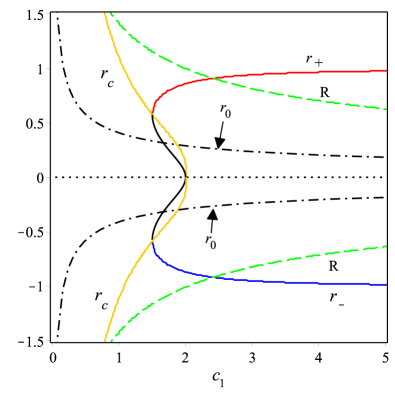
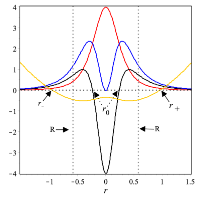
Figure 1: The behavior of $r_{\mp,0,c}$, and $R$ in terms of $c_{1}$ (left panel), and the behavior of $\rho$ (red), $\rho+P_{t}$ (blue), $\rho+P_{r}+P_{t}$ (black) and $f(r)$ (orange) in terms of $r$ (right panel) for the first black hole solution with the free parameters: $m=3/2,w_{1}=3,w_{2}=-2$, and $\rho_{0}=\ell=1$.

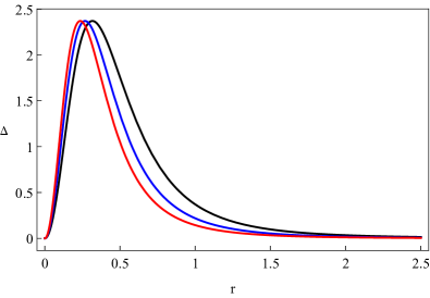
Figure 2: The behavior of $\Delta-r$ for the first black hole solution with the same numerical values used in Fig. 1. For the model parameter $c_{1}$, we have set numerical values $c_{1}=2.5,~{}3.5$, and $4.5$ in the black, blue, and red curves, respectively.

II.1 The first solution: $m=3/2$, $w_{1}=3$

To motivate the choices of constants, we notice that any value given to $m$ and $w_{1}$ leads to a possible solution. However, not all solutions yield a finite value for black hole mass. Hence, in our choices of constants, we present those values that provide a finite black hole mass.

Thus, inserting Eq. (16) into Eq. (13), one can obtain $f(r)$ as follows

$$f(r)=c_{2}+\dfrac{r^{2}}{\ell^{2}}+\dfrac{4\sqrt{\rho_{0}}}{c_{1}(4c_{1}\sqrt{\rho_{0}}r^{2}-w_{2})}.$$ (19)

This solution describes the gravitational field of a black hole if there exists an outer horizon located outside the radius of the compact object, i.e., $r_{+}>R$. The gravitational mass $M(r)$ inside a circle of radius $r$ is given by

$$M=2\pi\int_{0}^{\infty}r\rho(r)dr=-\dfrac{4\pi\sqrt{\rho_{0}}}{c_{1}\omega_{2}}.$$ (20)

We see that the central density depends on the square of the asymptotic value of the mass. Moreover, with the choice of constants that we made, a finite value of mass, as requested above, is found.

It is clear that both linear and power-law parts of $P_{t}(\rho)$ in Eq. (10) contribute to the gravitational mass so that it is positive ($M>0$) if $c_{1}\omega_{2}<0$ i.e., $\omega_{2}<0,c_{1}>0$, or $\omega_{2}>0,c_{1}<0$. If we assume that the above mass is equal to $M=\rho_{0}R^{2}$, then we obtain

$$R=\sqrt{-\dfrac{4\sqrt{\rho_{0}}}{c_{1}\omega_{2}\rho_{0}}},$$ (21)

which can be considered as the effective radius of the object. On the other hand, the roots of the metric function are given by

$$r_{\pm}= \pm\dfrac{1}{4c_{1}}\sqrt{\dfrac{2c_{1}\omega_{2}-8c_{2}\ell^{2}c_{1}^{2}\sqrt{\rho_{0}}\mp 2\sqrt{Y}}{\sqrt{\rho_{0}}}}$$ (22)

$$Y= c_{1}^{2}\omega_{2}^{2}+8c_{1}^{3}c_{2}\omega_{2}\ell^{2}\sqrt{\rho_{0}}+16\rho_{0}\ell^{4}c_{1}^{4}c_{2}^{2}-64\rho_{0}\ell^{2}c_{1}^{2},$$ (23)

where $r_{+}$ address the event horizon, while $r_{-}$ has no relation to the Cauchy horizon. For $c_{1}\gg 1$, the horizon radii are given as

$$r_{\pm}\sim\pm\ell\sqrt{-c_{2}}\mp\dfrac{\sqrt{-c_{2}}}{2\ell c_{1}^{2}c_{2}^{2}}+\mathcal{O}(c_{1}^{-3}),\;\;\;\;\;c_{1}\gg 1.$$ (24)

The extremal roots in which the roots degenerate to a single one are obtained as

$$r_{ext}=0,\pm\dfrac{1}{2}\sqrt{\dfrac{w_{2}+4\ell\sqrt{\rho_{0}}}{c_{1}\sqrt{\rho_{0}}}}.$$ (25)

This should not lead to the wrong interpretation that $r_{-}$ is Cauchy horizon. In general, this interpretation of $r_{\pm}$ is valid for the next two solutions, too. In the further analysis, We will not consider the case $w_{2}>0,c_{1}<0$, since $r_{ext}$ becomes imaginary. Fig. 1 (left panel) clearly shows that $r_{+}>R$ for $c_{1}$ bigger than a given value, indicating that the solution in Eq. (19) describes a 3D black hole.

To find the physical significance of the parameters $c_{1}$ and $c_{2}$, we consider the behavior of the solution (19). Hence, at $r\to\infty$ and $r\to 0$ we have

$$f(r)\sim c_{2}+\dfrac{r^{2}}{\ell^{2}}+\dfrac{1}{c_{1}^{2}r^{2}}+\mathcal{O}(r^{-4}),$$ (26)

and

$$f(r)\sim c_{2}-\dfrac{4\sqrt{\rho_{0}}}{c_{1}w_{2}}+\left(\dfrac{1}{\ell^{2}}-\dfrac{16\rho_{0}}{w_{2}^{2}}\right)r^{2}+\mathcal{O}(r^{4}),$$ (27)

respectively. By comparing the Eq. (26) with a static BTZ black hole, it is not hard to figure out that $c_{1}$ corresponds to a parameter with dimension $[c_{1}]=L^{-1}$ and $c_{2}$ is the dimensionless mass parameter $\mathcal{M}$. By re-expressing Eq. (27) in the following form

$$f(r)\sim c_{2}^{\prime}+\Lambda_{eff}r^{2}+\mathcal{O}(r^{4})$$ (28)

one can interpret the coefficient of $r^{2}$ in the form of an effective cosmological constant

$$\Lambda_{eff}=\dfrac{16\rho_{0}}{\omega_{2}^{2}}-\dfrac{1}{\ell^{2}}.$$ (29)

For $\omega_{2}^{2}/(16\rho_{0}\ell^{2})<1$, then $\Lambda_{eff}>0$, and $c^{\prime}_{2}=1$ indicating that the solution at hand near the origin is the dS vacuum. It is notable that the origin of the dS vacuum inside the black hole, in essence, comes from the power-law part of $P_{t}(\rho)$ in GPEoS, Eq. (10).

By calculating two curvature invariants, the Ricci and Kretschmann scalars, near the origin

$$\lim_{r\to 0}\mathcal{R}=-\dfrac{6}{\ell^{2}}+\dfrac{96\rho_{0}}{w_{2}^{2}}=6\Lambda_{eff},$$ (30)

$$\lim_{r\to 0}\mathcal{K}=\lim_{r\to 0}\mathcal{R}_{abcd}\mathcal{R}^{abcd}=\dfrac{12(-w_{2}^{2}+16\rho_{0}\ell^{2})^{2}}{\ell^{4}w_{2}^{4}}=12\Lambda_{eff}^{2},$$ (31)

one can see that they are finite at $r=0$, meaning that the first black hole solution is free of curvature singularities at the center. From Fig. 1 (right panel), one can conclude that the weak energy condition (WEC) i.e., $\rho>0$ and $\rho+P_{t}>0$ is satisfied everywhere, while the strong energy condition (SEC), $\rho+P_{r}+P_{t}>0$, is satisfied everywhere except at

$$r_{0}=\pm\dfrac{1}{6}\sqrt{\dfrac{-3w_{2}}{c_{1}\sqrt{\rho_{0}}}},$$ (32)

which is located near the origin. From the right panel of Fig. 1, it is also clearly evident that $r_{+}>R$. Equation (32) carries the message that the power-law part of $P_{t}(\rho)$ in GPEoS caused the SEC physics to be forced into a small region in the deep core i.e., $r<r_{0}$. This is interesting in the sense that it also happens in some regular 4D black holes so that one can take $r_{0}$ as a characteristic length associated with the Planck scale (e.g., see Carballo-Rubio:2018pmi ; Khodadi:2022dyi ).

As a double-check to ensure the existence of a vacuum near $r=0$, one can evaluate the anisotropic function $\Delta$ for the first solution. Indeed the anisotropic function is a suitable term to illustrate the internal structure of the black hole (or any relativistic stellar objects). The behavior of $\Delta-r$ in Fig. 2 clearly shows that although $\Delta$ reaches a maximum inside the black hole at a certain distance from the origin, it disappears as the center $r=0$ is approached, meaning that around the origin we are dealing with a vacuum.

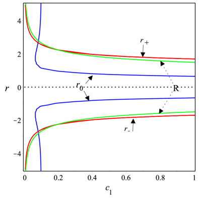
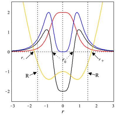
Figure 3: Same as Fig. 1 but for the second black hole solution with free parameters $m=2,\omega_{1}=3,\omega_{2}=-2$, and $\rho_{0}=\ell=1$.

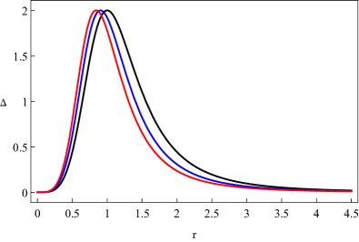
Figure 4: The behavior of $\Delta-r$ for the second black hole solution with the same numerical values used in Fig. 3. For the model parameter $c_{1}$, we have set numerical values $c_{1}=0.5,~{}0.75$, and $1$ in the black, blue, and red curves, respectively.

According to Appendix A, the computation of the curvature eigenvalues, $\lambda_{i}$, for this metric yields

$$\lambda_{1} =\dfrac{1}{\ell^{2}(4c_{1}\sqrt{\rho_{0}}r^{2}-\omega_{2})^{3}}[64c_{1}^{3}\rho_{0}^{\frac{3}{2}}r^{6}-48c_{1}^{2}\rho_{0}\omega_{2}r^{4}+$$

$$12c_{1}\omega_{2}^{2}r^{2}\sqrt{\rho_{0}}-\omega_{2}^{3}+192c_{1}\ell^{2}r^{2}\rho_{0}^{\frac{3}{2}}+16\rho_{0}\omega_{2}\ell^{2}]$$ (33)

$$\lambda_{2}= -\lambda_{3}=\dfrac{16c_{1}^{2}\rho_{0}r^{4}-8c_{1}\omega_{2}\sqrt{\rho_{0}}r^{2}+\omega_{2}^{2}-16\rho_{0}\ell^{2}}{\ell^{2}(4c_{1}r^{2}\sqrt{\rho_{0}}-\omega_{2})^{2}}$$ (34)

For $r\to\infty$, then $\lambda_{1}=\lambda_{2}=-\lambda_{3}=1/\ell^{2}$. The first extremum that is reached when approaching from infinity is located at $r_{rep}=\pm\sqrt{-\omega_{2}c_{1}\rho_{0}^{\frac{3}{2}}}/(2c_{1}\rho_{0})$ which corresponds to a local maximum of $\lambda_{2}$ and determines the place of the repulsion onset. On the other hand, $\lambda_{1}$ and $\lambda_{2}$ change sign at

$$r^{(1)}_{dom}= \pm\sqrt{\dfrac{\omega_{2}+4\ell\sqrt{\rho_{0}}}{4c_{1}\sqrt{\rho_{0}}}},$$ (35)

$$r^{(2)}_{dom}= \dfrac{1}{2\sqrt{c_{1}}}\sqrt{\dfrac{\omega_{2}}{\sqrt{\rho_{0}}}+2(4B)^{\frac{1}{3}}-2\ell^{2}(\dfrac{16}{B})^{\frac{1}{3}}},$$ (36)

where

$$B=\dfrac{\ell^{2}}{\sqrt{\rho_{0}}}\left(-\omega_{2}+\sqrt{\omega_{2}^{2}+4\rho_{0}\ell^{2}}\right).$$ (37)

According to our definition, we take the greatest value (the first zero from infinity) as indicating the region where repulsion dominates, i.e., $r_{dom}^{(2)}$. The weak energy condition turns out to be identically satisfied for $r>0$. However, the strong energy condition is also violated at the radius $r_{0}$. Notice the interesting relationship $r_{0}=r_{rep}/\sqrt{3}$, indicating that the repulsion radius can be associated with the location, where the strong energy condition is violated. We conclude that the onset and dominance region of repulsive gravity occur at radii close to the origin of coordinates. This result indicates that repulsion can be considered as inducing the regular behavior of the curvature at the center of the black hole.

II.2 The second solution: $m=2,w_{1}=3$

Again the underlying choice refers to the need of constant black hole mass. Specifically, for this case, the lapse function in Eq. (1) is represented as follows

$$f(r)=c_{2}+\dfrac{r^{2}}{\ell^{2}}+\dfrac{2\rho_{0}}{\sqrt{c_{1}w_{2}\rho_{0}}}\arctan\left(\dfrac{2c_{1}\rho_{0}r^{2}}{\sqrt{c_{1}w_{2}\rho_{0}}}\right).$$ (38)

The gravitational mass $M$ for a 2D sphere of radius $r$ becomes

$$M=2\pi\int_{0}^{\infty}r\rho(r)dr=-\dfrac{\pi^{2}\sqrt{-w_{2}\rho_{0}}}{\sqrt{c_{1}}w_{2}},$$ (39)

which results in the following effective radius

$$R=\pm\sqrt{-\dfrac{\pi\sqrt{-w_{2}\rho_{0}}}{\sqrt{c_{1}}w_{2}}}.$$ (40)

For the effective radius above to make sense, i.e., $R>0$, we should demand $w_{2}<0$. The roots of the equation $f(r)=0$ determine the horizons of the above solution. In particular, the extremal root is obtained as

$$r_{ext}=\dfrac{\big{(}\rho_{0}^{3}c_{1}^{3}(w_{2}+4\rho_{0}\ell^{2})\big{)}^{\frac{1}{4}}}{\sqrt{2}c_{1}\rho_{0}}.$$ (41)

The left panel of Fig. 3 openly shows that $r_{+}>R$ for a large range of values of $c_{1}$, meaning that the solution in Eq. (38) represents a 3D black hole solution. Moreover, the curve $f(r)$ in the right panel also confirms that the second solution addresses a black hole (since $r_{+}>R$).

Regarding the asymptotic behavior of the metric (38) at $r\to\infty$ and $r\to 0$, we have

$$f(r)\sim c_{2}+\dfrac{\pi\sqrt{-\rho_{0}\omega_{2}}}{\sqrt{c_{1}}(-\omega_{2})^{\frac{3}{2}}}+\dfrac{r^{2}}{\ell^{2}}+\dfrac{1}{c_{1}r^{2}}+\mathcal{O}(r^{-6}),$$ (42)

and

$$f(r)\sim c_{2}+\left(\dfrac{1}{\ell^{2}}+\dfrac{4\rho_{0}}{\omega_{2}}\right)r^{2}+\mathcal{O}(r^{6}),$$ (43)

respectively. Unlike the first solution, here $c_{2}$ singly does not play the role of mass, but the term $c_{2}+\frac{\pi\sqrt{-\rho_{0}\omega_{2}}}{\sqrt{c_{1}}(-\omega_{2})^{\frac{3}{2}}}=-\mathcal{M}$, which is effectively associated with the ADT mass of the configuration. The relation in Eq. (43) explicitly shows that, for the second solution, the effective cosmological constant is

$$\Lambda_{eff}=-\dfrac{1}{\ell^{2}}-\dfrac{4\rho_{0}}{\omega_{2}},$$ (44)

which is positive for $\frac{4\rho_{0}\ell^{2}}{\mid\omega_{2}\mid}>1$. In addition, the choice $c_{2}=1$ indicates the presence of dS core, which is a direct consequence of the power-law part of $P_{t}(\rho)$ in Eq. (10).

In the same manner, the Ricci and Kretschmann scalars are both finite everywhere i.e.,

$$\lim_{r\to 0}\mathcal{R}= -\dfrac{6}{\ell^{2}}-\dfrac{24\rho_{0}}{w_{2}}=6\Lambda_{eff},$$ (45)

$$\lim_{r\to 0}\mathcal{K}= \dfrac{12(w_{2}+4\rho_{0}\ell^{2})^{2}}{\ell^{4}w_{2}^{2}}=12\Lambda_{eff}^{2},$$ (46)

Similar to the first solution, from the right panel in Fig. 3, one can conclude that the transverse WEC is met everywhere, while the SEC works for regions $r>r_{0}$

$$r_{0}=\pm\left({\dfrac{-w_{2}}{12c_{1}{\rho_{0}}}}\right)^{\frac{1}{4}},$$ (47)

namely, everywhere within the dS core except for the region near the origin with radius $r_{0}$.

As before, Fig. 4 shows that around the origin the value of the anisotropic function vanishes, meaning that there is a vacuum in the center of the second solution.

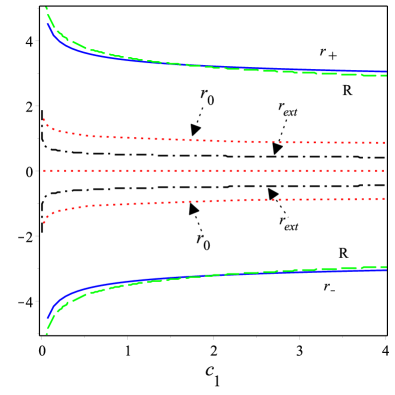
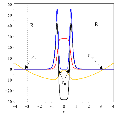
Figure 5: Same as Fig. 1 but for the third black hole solution with free parameters $m=2,\omega_{1}=7,\omega_{2}=-1$, and $\rho_{0}=3.5$

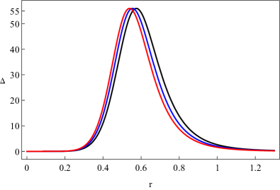
Figure 6: The behavior of $\Delta-r$ for the third black hole solution with the same numerical values used in Fig. 5. For the model parameter $c_{1}$, we have set numerical values $c_{1}=3,~{}3.5$, and $4$ in the black, blue, and red curves, respectively.

Computing the curvature eigenvalues $\lambda_{i}$ for this metric, according to Appendix A, we can write

$$\lambda_{1} =\dfrac{\omega_{2}^{2}-8\omega_{2}c_{1}\rho_{0}r^{4}+16c_{1}^{2}\rho_{0}^{2}r^{8}+4\rho_{0}\omega_{2}\ell^{2}+48\rho_{0}^{2}c_{1}\ell^{2}r^{4}}{\ell^{2}(4c_{1}\rho_{0}r^{4}-\omega_{2})^{2}}$$

$$\lambda_{2} =-\lambda_{3}=\dfrac{\rho_{0}(4c_{1}r^{4}-4\ell^{2})-\omega_{2}}{\ell^{2}(4c_{1}\rho_{0}r^{4}-\omega_{2})^{2}}$$ (48)

The first extremum that is reached when approaching from infinity is located at $r_{rep}=\pm\frac{1}{c_{1}\rho_{0}}\left(\frac{-5\omega_{2}c_{1}^{3}\rho_{0}^{3}}{12}\right)^{\frac{1}{4}}$ which corresponds to a local maximum of $\lambda_{1}$. On the other hand, $\lambda_{1}$ and $\lambda_{2}$ change sign at

$$r^{(1)}_{dom}= \pm\frac{\left(c_{1}^{3}\rho_{0}^{3}(\omega_{2}+4\rho_{0}\ell^{2})\right)^{\frac{1}{4}}}{\sqrt{2}c_{1}\rho_{0}},$$ (49)

$$r^{(2)}_{dom}= \dfrac{(-c_{1}^{3}\rho_{0}^{3}(-\omega_{2}+6\rho_{0}\ell^{2}-2\sqrt{9\rho_{0}^{2}\ell^{4}-4\rho_{0}\omega_{2}\ell^{2}}))^{\frac{1}{4}}}{\sqrt{2}c_{1}\rho_{0}}.$$ (50)

According to our definition, the greatest value indicates the region where repulsion dominates, i.e. $r^{(1)}_{dom}$. The WEC turns out to be identically satisfied for $r>0$. However, the SEC is violated at the radius $r_{0}$. As in the previous case, we find a relationship between the repulsion radius and the location where the SEC is violated, i.e, $r_{0}=r_{rep}/\sqrt{5}$.

II.3 The third solution: $m=2$, $w_{1}=7$

Guaranteeing a suitable choice of constant that leads to a constant black hole mass, as above, we here find the lapse function to read

$$f(r)= c_{2}+\dfrac{r^{2}}{\ell^{2}}+\dfrac{\rho_{0}A^{\frac{1}{4}}}{\sqrt{2}w_{2}}\ln\left[\dfrac{2r^{4}+\sqrt{2}r^{2}A^{\frac{1}{4}}+\dfrac{\sqrt{A}}{2}}{2r^{4}-\sqrt{2}r^{2}A^{\frac{1}{4}}+\dfrac{\sqrt{A}}{2}}\right]$$ (51)

$$+\dfrac{\sqrt{2}\rho_{0}A^{\frac{1}{4}}}{w_{2}}\arctan\left(\dfrac{2\sqrt{2}r^{2}A^{\frac{1}{4}}}{A^{\frac{1}{2}}-4r^{4}}\right),$$

where $A=-2w_{2}/c_{1}\rho_{0}$. For a 2D sphere of radius $r$, the gravitational mass $M$ and relevant effective radius $R$ can be expressed as follows

$$M=2\pi\int_{0}^{\infty}r\rho(r)dr=\dfrac{\pi^{2}(2\rho_{0})^{\frac{3}{4}}}{c_{1}^{\frac{1}{4}}(-w_{2})^{\frac{3}{4}}},$$ (52)

and

$$R=\pm\dfrac{\pi}{c_{1}^{\frac{1}{8}}}\left(\dfrac{2}{-w_{2}\rho_{0}}\right)^{\frac{3}{8}}.$$ (53)

As in the previous two cases, here we also need $c_{1}>0$ and $w_{2}<0$. Unlike the previous two cases, the lapse function in Eq. (51) does not allow to present analytical expressions for $r_{\pm}$, and $r_{ext}$. Hence, we extract them in a numerical manner in Fig. 5, from which it is evident, and also from the behavior of $f(r)$ shown in the right panel, that the third solution represents a 3D black hole solution.

The behavior of the lapse function (51) as $r\to\infty$ and $r\to 0$ is

$$f(r)\sim c_{2}+\dfrac{r^{2}}{\ell^{2}}+\dfrac{\sqrt{2}\pi\rho_{0}A^{\frac{1}{4}}}{w_{2}}+\mathcal{O}(r^{-6}),$$ (54)

and

$$f(r)\sim c_{2}+\left(\dfrac{1}{\ell^{2}}+\dfrac{8\rho_{0}}{w_{2}}\right)r^{2}+\mathcal{O}(r^{3}),$$ (55)

respectively. First, Eq. (54) implies that the asymptotic limit of the third solution meets the lapse function of static BTZ black hole solution provided that $c_{2}+\frac{\sqrt{2}\pi\rho_{0}A^{\frac{1}{4}}}{w_{2}}=-\mathcal{M}$. Given that the gravitational mass is dimensionless, so it can be easily recognized that $[c_{1}]=L^{-6}$, and $c_{2}$ is dimensionless. Second, one can interpret the coefficient of $r^{2}$ in Eq. (55) as an effective cosmological constant as

$$\Lambda_{eff}=-\left(\dfrac{1}{\ell^{2}}+\dfrac{8\rho_{0}}{w_{2}}\right).$$ (56)

As before, one can show that the Kretschmann and Ricci scalars are finite at the center of the black hole since

$$\lim_{r\to 0}\mathcal{R}=6\Lambda_{eff},$$ (57)

$$\lim_{r\to 0}\mathcal{K}=\lim_{r\to 0}\mathcal{R}_{abcd}\mathcal{R}^{abcd}=12\Lambda_{eff}^{2}.$$ (58)

Here, as in the previous two cases, from Fig. 5 (right panel) one can conclude that the WEC is satisfied everywhere, while the SEC is satisfied everywhere except near the origin at

$$r_{0}=\pm\Big{(}\frac{-c_{1}^{3}\rho_{0}^{3}w_{2}}{56}\Big{)}^{1/8}(c_{1}\rho_{0})^{-1/2}.$$ (59)

The equation above explicitly tells us that the GPEoS (10) results in pushing the SEC physics into a small region deep in core, i.e., $r<r_{0}$, just like the previous ones.

It is evident from Fig. 7 that the third black hole solution around the center $r=0$ corresponds to a vacuum (i.e., $\Delta=0$), as in the previous two cases.

Now we analyze the behavior of repulsive gravity in this black hole. The curvature eigenvalues, $\lambda_{i}$, are given in terms of cumbersome expressions that cannot be represented in a compact form. However, a numerical study shows that the radii $r_{rep}$ and $r_{dom}$ are located in a region close to the center, as depicted in Fig. 7.

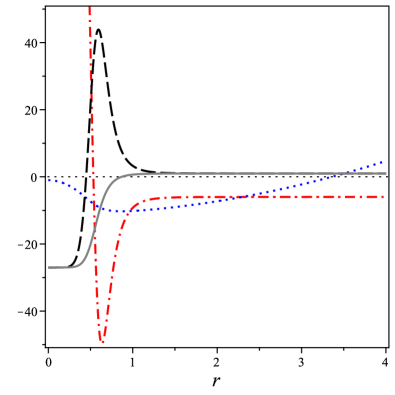
Figure 7: Plots of the eigenvalues, $\lambda_{1}$, $\lambda_{2}$ and $f(r)$, $R$ for the third solution for $c_{1}=3,\ell=1,\rho_{0}=3.5,\omega_{2}=-1$.

We see that the eigenvalues are finite everywhere. The main result is that repulsive gravity is present in both eigenvalues and, in fact, it becomes the dominant component as the origin of coordinates is approached, forcing the eigenvalues to become finite at $r=0$. Thus, we conclude that the regular behavior of this black hole is a consequence of the presence of repulsive gravity.

Let us close this section by mentioning an important point. Apart from the analytic solutions presented above, the existing setup allows large numbers of non-black hole solutions, which are obtained by setting other values for $m$ and $w_{1}$. However, we limit ourselves to pointing to one of them since the non-black hole solutions are beyond the scope of this work. For instance, setting the values $m=2,w_{1}=1$, we obtain a solution in which the total mass and, subsequently, the radius diverge from the view of an observer at infinity, meaning that this solution is unbounded and cannot represent a black hole.

III Conclusion

Considering an anisotropic relativistic configuration of polytropes, described by the GPEoS, Eq. (10), in a 3D static background, we first generalized the TOV equations in order to derive compatible solutions.

We found out that the structure of the anisotropic pressure consists of radial and transverse components, exhibiting vacuum energy and a GPEoS with a linear term plus a power-law contribution. This scenario is widely-adopted in astrophysical contexts since it is thought to well-approximate real compact objects.

Consequently, we solved the full system of existing equations via setting certain values for the model parameters denoted as $m$, $c_{1}$, and $c_{2}$. Thus, we derived three analytical black hole solutions prompting a dS core, i.e., being regular at $r=0$ and smoothly approaching an asymptotically AdS spacetime.

The status of the WEC and SEC was discussed for the three main solutions, by varying the above parameters. We underlined that both WEC and SEC are satisfied everywhere with the remarkable exception of the SEC that is violated in a small region inside the dS core. Physically, the existence of a dS core can be interpreted as the absence of singularity, suggesting the black hole to be regular.

Inspired by other regular 4D black holes with a dS core, such a length scale depth in the core has been related to the fundamental Planck length.

Furthermore, by analyzing the behavior of the curvature eigenvalues, we demonstrated that repulsive gravity is present near the center of the black holes and it can interpreted as being responsible or the avoidance of curvature singularities. Thus, we can conclude that the regularity property of the analyzed black holes is due to the presence of repulsive gravity.

As a perspective, we notice that these solutions can be further investigated, for instance, regarding the dynamic stability of these solutions against superradiance scattering, as well as concerning their asymptotic symmetry and the conformal field theory in $AdS_{3}$ (following the observations of Brown and Heno, Ref. Brown:1986nw ).

Appendix A Repulsive gravity

In this Appendix, we review an invariant formalism for describing repulsive gravity in terms of the eigenvalues of the Riemman curvature tensor.

To obtain the Riemann curvature tensor in a local orthonormal frame, we choose the orthonormal tetrad $e^{a}$ as

$$ds^{2}=\eta_{ab}e^{a}\otimes e^{b}$$ (60)

with $\eta_{ab}=diag(-1,1,1)$. The first

$$de^{a}+\omega^{a}{}_{b}\wedge e^{b}=0$$ (61)

and second Cartan structure equations

$$\Omega^{a}{}_{b}=d\omega^{a}{}_{b}+\omega^{a}{}_{c}\wedge\omega^{c}{}_{b}=\dfrac{1}{2}R^{a}{}_{bcd}e^{c}\wedge e^{d},$$ (62)

allow us to introduce the connection 1-form $\omega^{a}_{\ b}$ and the curvature 2-form $\Omega^{a}_{\ b}$, which determines the tetrad components of the curvature tensor $R^{a}_{\ bcd}$.

Furthermore, to compute the curvature eigenvalues, it is convenient to introduce the convention

$$1\to 12,\;\;\;\;2\to 13,\;\;\;3\to 23.$$ (63)

Then, the curvature eigenvalues are easily computed as the eigenvalues of the matrix $R_{AB}$.

Consider now the case of a spacetime geometry in circularly symmetric 3D with coordinates ($t,r,\phi$),

$$ds^{2}=-f(r)dt^{2}+\dfrac{dr^{2}}{f(r)}+r^{2}d\phi^{2}\;,$$ (64)

where $t,r\in R$, $\phi\in[0,2\pi]$. Therefore, we have

$$e^{1}=\sqrt{f}dt,\;\;\;e^{2}=\dfrac{dr}{\sqrt{f}},\;\;\;e^{3}=rd\phi$$ (65)

The components of the connection 1-form are determined using (61), as follows

$$\omega^{1}{}_{2}=\dfrac{f^{\prime}}{2\sqrt{f}}e^{1},\;\;\;\omega^{2}{}_{3}=-\dfrac{\sqrt{f}}{r}e^{3}\ .$$ (66)

Moreover, using equation (62), we obtain

$$R_{1212}=\dfrac{f^{\prime\prime}}{2},\;\;\;\;R_{1313}=\dfrac{f^{\prime}}{2r},\;\;\;R_{2323}=-\dfrac{f^{\prime}}{2r}.$$ (67)

Finally, according to the convention (63), the ($3\times 3$)-matrix $R_{AB}$ can be written as

$$R_{AB}=\begin{bmatrix}\dfrac{f^{\prime\prime}}{2}&0&0\\ 0&\dfrac{f^{\prime}}{2r}&0\\ 0&0&-\dfrac{f^{\prime}}{2r}\end{bmatrix}$$

Therefore, the curvature eigenvalues, $\lambda_{i}$, are given by Luongo:2023xaw ; Luongo:2023aib ; Luongo:2014qoa ,

$$\lambda_{1}=\dfrac{f^{\prime\prime}}{2},\;\;\;\lambda_{2}=\dfrac{f^{\prime}}{2r},\;\;\;\lambda_{3}=-\dfrac{f^{\prime}}{2r}.$$ (68)

These eigenvalues encapsulate all the information regarding curvature and exhibit scalar behavior under coordinate transformations. The identification of repulsive gravity is established as follows: The change in sign of at least one eigenvalue signifies the transition to repulsive gravity, meaning the zeros of the eigenvalues mark the locations where repulsive gravity becomes predominant.

The existence of an extremum in an eigenvalue indicates the initiation of repulsive gravity, with the onset determined by the condition

$$\partial\lambda_{i}/\partial r=0.$$ (69)

References

- (1) J. R. Gott and M. Alpert, Gen. Rel. Grav. 16, 243-247 (1984)
- (2) S. Giddings, J. Abbott and K. Kuchar, Gen. Rel. Grav. 16, 751-775 (1984)
- (3) S. Deser, R. Jackiw and G. ’t Hooft, Annals Phys. 152, 220 (1984)
- (4) S. Deser and R. Jackiw, Annals Phys. 153, 405-416 (1984)
- (5) J. D. Brown and M. Henneaux, Commun. Math. Phys. 104, 207-226 (1986)
- (6) E. Witten, Nucl. Phys. B 311, 46 (1988)
- (7) R. B. Mann, Gen. Rel. Grav. 24, 433-449 (1992)
- (8) R. B. Mann, [arXiv:gr-qc/9501038 [gr-qc]].
- (9) E. Elizalde and S. D. Odintsov, Nucl. Phys. B 399, 581-600 (1993) [arXiv:hep-th/9207046 [hep-th]].
- (10) S. Carlip, “Quantum Gravity in 2+1 Dimensions”, Cambridge University Press, (1998)
- (11) A. Vilenkin and E.P.S. Shellard, “Cosmic Strings and Other Topological Defects”, Cambridge University Press, (2000).
- (12) A. Achucarro and P. K. Townsend, Phys. Lett. B 180, 89 (1986)
- (13) J. D. Barrow, A. B. Burd, and D. Lancaster, Class. Quant. Grav. 3 551 (1986).
- (14) S. Deser, R. Jackiw and S. Templeton, Annals Phys. 140, 372-411 (1982) [erratum: Annals Phys. 185, 406 (1988)]
- (15) E. A. Bergshoeff, O. Hohm and P. K. Townsend, Phys. Rev. Lett. 102, 201301 (2009) [arXiv:0901.1766 [hep-th]].
- (16) E. Bergshoeff, O. Hohm, W. Merbis, A. J. Routh and P. K. Townsend, Class. Quant. Grav. 31, 145008 (2014) [arXiv:1404.2867 [hep-th]].
- (17) M. R. Setare, Nucl. Phys. B 898, 259-275 (2015) [arXiv:1412.2151 [hep-th]].
- (18) M. Özkan, Y. Pang and P. K. Townsend, JHEP 08, 035 (2018) [arXiv:1806.04179 [hep-th]].
- (19) D. Ida, Phys. Rev. Lett. 85, 3758-3760 (2000) [arXiv:gr-qc/0005129 [gr-qc]].
- (20) A. Bagchi, S. Detournay, D. Grumiller and J. Simon, Phys. Rev. Lett. 111, no.18, 181301 (2013) [arXiv:1305.2919 [hep-th]].
- (21) M. R. Setare and S. N. Sajadi, Class. Quant. Grav. 38, no.14, 145009 (2021) [arXiv:2012.00002 [gr-qc]].
- (22) M. Banados, C. Teitelboim and J. Zanelli, Phys. Rev. Lett. 69, 1849-1851 (1992) [arXiv:hep-th/9204099 [hep-th]].
- (23) C. Martinez, C. Teitelboim and J. Zanelli, Phys. Rev. D 61, 104013 (2000) [arXiv:hep-th/9912259 [hep-th]].
- (24) O. J. C. Dias and J. P. S. Lemos, JHEP 01, 006 (2002) [arXiv:hep-th/0201058 [hep-th]].
- (25) S. Carlip, Phys. Rev. D 51, 632-637 (1995) [arXiv:gr-qc/9409052 [gr-qc]].
- (26) M. Banados, M. Henneaux, C. Teitelboim and J. Zanelli, Phys. Rev. D 48, 1506-1525 (1993) [erratum: Phys. Rev. D 88, 069902 (2013)] [arXiv:gr-qc/9302012 [gr-qc]].
- (27) N. R. Pantoja, H. Rago and R. O. Rodriguez, J. Math. Phys. 45, 1994-2002 (2004) [arXiv:gr-qc/0205094 [gr-qc]].
- (28) B. Chen, F. L. Lin and B. Ning, Phys. Rev. D 100, no.4, 044043 (2019) [arXiv:1902.00949 [gr-qc]].
- (29) S. Carlip, Class. Quant. Grav. 12, 2853-2880 (1995) [arXiv:gr-qc/9506079 [gr-qc]].
- (30) Á. Rincón and G. Panotopoulos, Phys. Rev. D 97, no.2, 024027 (2018) [arXiv:1801.03248 [hep-th]].
- (31) G. Panotopoulos and A. Rincón, Phys. Rev. D 97, no.8, 085014 (2018) [arXiv:1804.04684 [hep-th]].
- (32) J. Podolsky, R. Svarc and H. Maeda, Class. Quant. Grav. 36, no.1, 015009 (2019) [arXiv:1809.02480 [gr-qc]].
- (33) M. Sharif and S. Sadiq, Chin. J. Phys. 60, 279-289 (2019)
- (34) A. Ali and K. Saifullah, Eur. Phys. J. C 82, no.2, 131 (2022)
- (35) S. Priyadarshinee and S. Mahapatra, [arXiv:2305.09172 [gr-qc]].
- (36) T. Karakasis, G. Koutsoumbas and E. Papantonopoulos, Phys. Rev. D 107, no.12, 124047 (2023) [arXiv:2305.00686 [gr-qc]].
- (37) J. Parsons and S. F. Ross, JHEP 04, 134 (2009) [arXiv:0901.3044 [hep-th]].
- (38) R. A. Hennigar, D. Kubiznak, R. B. Mann and C. Pollack, Phys. Lett. B 808, 135657 (2020) [arXiv:2004.12995 [gr-qc]].
- (39) R. A. Hennigar, D. Kubiznak and R. B. Mann, Class. Quant. Grav. 38, no.3, 03LT01 (2021) [arXiv:2005.13732 [gr-qc]].
- (40) A. Sheykhi, JHEP 01, 043 (2021) [arXiv:2009.12826 [gr-qc]].
- (41) E. F. Eiroa and G. Figueroa-Aguirre, Phys. Rev. D 103, no.4, 044011 (2021) [arXiv:2011.14952 [gr-qc]].
- (42) T. Karakasis, E. Papantonopoulos, Z. Y. Tang and B. Wang, Phys. Rev. D 103, no.6, 064063 (2021) [arXiv:2101.06410 [gr-qc]].
- (43) G. G. L. Nashed and A. Sheykhi, Phys. Dark Univ. 40, 101174 (2023) [arXiv:2110.02071 [physics.gen-ph]].
- (44) T. Karakasis, E. Papantonopoulos, Z. Y. Tang and B. Wang, Phys. Rev. D 105, no.4, 044038 (2022) [arXiv:2201.00035 [gr-qc]].
- (45) K. C. K. Chan and R. B. Mann, Phys. Rev. D50 6385 (1994)
- (46) E. Witten, [arXiv:0706.3359 [hep-th]].
- (47) D. Birmingham, I. Sachs and S. N. Solodukhin, Phys. Rev. Lett. 88, 151301 (2002) [arXiv:hep-th/0112055 [hep-th]].
- (48) J. Ren, JHEP 11, 055 (2010) [arXiv:1008.3904 [hep-th]].
- (49) D. Momeni, H. Gholizade, M. Raza and R. Myrzakulov, Phys. Lett. B 747, 417-425 (2015) [arXiv:1503.02896 [hep-th]].
- (50) L. Eberhardt, M. R. Gaberdiel and R. Gopakumar, JHEP 02, 136 (2020) [arXiv:1911.00378 [hep-th]].
- (51) L. Eberhardt, JHEP 05, 150 (2020) [arXiv:2002.11729 [hep-th]].
- (52) B. Balthazar, A. Giveon, D. Kutasov and E. J. Martinec, JHEP 01, 008 (2022) [arXiv:2109.00065 [hep-th]].
- (53) G. Clement, Phys. Lett. B 367, 70-74 (1996) [arXiv:gr-qc/9510025 [gr-qc]].
- (54) M. Cadoni and M. R. Setare, JHEP 07, 131 (2008) [arXiv:0806.2754 [hep-th]].
- (55) H. Quevedo and A. Sanchez, Phys. Rev. D 79, 024012 (2009) [arXiv:0811.2524 [gr-qc]].
- (56) Y. Liu, Q. Pan and B. Wang, Phys. Lett. B 702, 94-99 (2011) [arXiv:1106.4353 [hep-th]].
- (57) S. H. Hendi, JHEP 03, 065 (2012) [arXiv:1405.4941 [hep-th]].
- (58) A. Sheykhi, S. H. Hendi and S. Salarpour, Phys. Scripta 10, 105003 (2014)
- (59) H. R. C. Ferreira and C. A. R. Herdeiro, Phys. Lett. B 773, 129-134 (2017) [arXiv:1707.08133 [gr-qc]].
- (60) C. Dappiaggi, H. R. C. Ferreira and C. A. R. Herdeiro, Phys. Lett. B 778, 146-154 (2018) [arXiv:1710.08039 [gr-qc]].
- (61) M. Fujita and J. Zhang, Phys. Rev. D 107, no.2, 026007 (2023) [arXiv:2205.06964 [hep-th]].
- (62) C. C. de Oliveira and R. A. Mosna, Phys. Rev. D 106, no.6, 064030 (2022) [arXiv:2206.01147 [gr-qc]].
- (63) R. R. Poojary, Phys. Rev. D 107, no.6, 066019 (2023) [arXiv:2209.03065 [hep-th]].
- (64) J. Furtado and G. Alencar, Universe 8, no.12, 625 (2022) [arXiv:2210.06608 [gr-qc]].
- (65) Y. Yu, J. Zhang and H. Yu, JHEP 03, 209 (2023) [arXiv:2212.02820 [hep-th]].
- (66) I. Basile, A. Campoleoni and J. Raeymaekers, JHEP 03, 187 (2023) [arXiv:2301.11883 [hep-th]].
- (67) O. Baake and J. Zanelli, Phys. Rev. D 107, no.8, 084015 (2023) [arXiv:2301.04256 [hep-th]].
- (68) S. Konewko and E. Winstanley, [arXiv:2301.01169 [hep-th]].
- (69) Y. Du and X. Zhang, [arXiv:2302.11189 [gr-qc]].
- (70) Y. T. Zhou, [arXiv:2302.10565 [hep-th]].
- (71) L. Chen, H. Zhang and B. Zhang, Commun. Theor. Phys. 75, no.3, 035302 (2023) [arXiv:2303.15661 [gr-qc]].
- (72) S. G. Devi, I. A. Meitei, T. I. Singh, A. K. Singh and K. Y. Singh, Int. J. Mod. Phys. A 38, no.12n13, 2350068 (2023) [arXiv:2304.12359 [gr-qc]].
- (73) H. S. Jeong, C. W. Ji and K. Y. Kim, [arXiv:2306.14805 [hep-th]].
- (74) R. D. B. Fontana, [arXiv:2306.02504 [gr-qc]].
- (75) Y. He and M. S. Ma, Phys. Lett. B 774, 229-234 (2017) [arXiv:1709.09473 [gr-qc]].
- (76) M. Cataldo and A. Garcia, Phys. Rev. D 61, 084003 (2000) [arXiv:hep-th/0004177 [hep-th]].
- (77) Y. S. Myung and M. Yoon, Eur. Phys. J. C 62, 405-411 (2009) [arXiv:0810.0078 [gr-qc]].
- (78) P. Bueno, P. A. Cano, J. Moreno and G. van der Velde, Phys. Rev. D 104, no.2, L021501 (2021) [arXiv:2104.10172 [gr-qc]].
- (79) K. Jusufi, [arXiv:2209.04433 [gr-qc]].
- (80) K. Jusufi, M. Jamil, A. Sheykhi [arXiv:2302.10799 [gr-qc]].
- (81) T. Karakasis, N. E. Mavromatos and E. Papantonopoulos, Phys. Rev. D 108, no.2, 024001 (2023) [arXiv:2305.00058 [gr-qc]].
- (82) P. H. Chavanis, Eur. Phys. J. Plus 129, 38 (2014) [arXiv:1208.0797 [astro-ph.CO]].
- (83) P. H. Chavanis, Eur. Phys. J. Plus 129, no.10, 222 (2014) [arXiv:1208.0801 [astro-ph.CO]].
- (84) S. N. Sajadi and N. Riazi, Can. J. Phys. 98, no.11, 1046-1054 (2020) [arXiv:1611.04343 [gr-qc]].
- (85) N. Riazi, S. S. Hashemi, S. N. Sajadi and S. Assyyaee, Can. J. Phys. 94, no.10, 1093-1101 (2016) [arXiv:1507.03420 [gr-qc]].
- (86) S. Chandrasekha, An introduction to the study of stellar structure (New York: Dover) (2010)
- (87) L. Herrera and W. Barreto, Phys. Rev. D 88, no.8, 084022 (2013) [arXiv:1310.1114 [gr-qc]].
- (88) P. M. Sa, Phys. Lett. B 467, 40 (1999) [arXiv:gr-qc/0302074 [gr-qc]].
- (89) U. S. Nilsson and C. Uggla, Annals Phys. 286, 292-319 (2001) [arXiv:gr-qc/0002022 [gr-qc]].
- (90) H. Maeda, T. Harada, H. Iguchi and N. Okuyama, Phys. Rev. D 66, 027501 (2002) [arXiv:gr-qc/0204039 [gr-qc]].
- (91) X. Y. Lai and R. X. Xu, Astropart. Phys. 31, 128-134 (2009) [arXiv:0804.0983 [astro-ph]].
- (92) M. R. Setare and H. Adami, Phys. Rev. D 91, no.8, 084014 (2015)
- (93) E. Contreras, Á. Rincón, B. Koch and P. Bargueño, Eur. Phys. J. C 78, no.3, 246 (2018) [arXiv:1803.03255 [gr-qc]].
- (94) G. Abellan, E. Fuenmayor, E. Contreras and L. Herrera, Phys. Dark Univ. 30, 100632 (2020) [arXiv:2007.00193 [gr-qc]].
- (95) F. Shojai, A. Sadeghi and R. Hassannejad, Class. Quant. Grav. 39, no.8, 085003 (2022) [arXiv:2202.14024 [gr-qc]].
- (96) J. P. Mimoso, M. Le Delliou and F. C. Mena, Phys. Rev. D 88, 043501 (2013) [arXiv:1302.6186 [gr-qc]].
- (97) P. H. Nguyen and M. Lingam, Mon. Not. Roy. Astron. Soc. 436, 2014-2028 (2013) [arXiv:1307.8433 [gr-qc]].
- (98) A. Drago, A. Lavagno and G. Pagliara, Phys. Rev. D 71, 103004 (2005) [arXiv:astro-ph/0312009 [astro-ph]].
- (99) L. Herrera, A. Di Prisco, J. Martin, J. Ospino, N. O. Santos and O. Troconis, Phys. Rev. D 69, 084026 (2004) [arXiv:gr-qc/0403006 [gr-qc]].
- (100) M. Cadoni, A. P. Sanna and M. Tuveri, Phys. Rev. D 102, no.2, 023514 (2020) [arXiv:2002.06988 [gr-qc]].
- (101) R. C. Freitas and S. V. B. Goncalves, Eur. Phys. J. C 74, no.12, 3217 (2014) [arXiv:1310.2917 [astro-ph.CO]].
- (102) R. Carballo-Rubio, F. Di Filippo, S. Liberati, C. Pacilio and M. Visser, JHEP 07, 023 (2018) [arXiv:1805.02675 [gr-qc]].
- (103) M. Khodadi and R. Pourkhodabakhshi, Phys. Rev. D 106, no.8, 084047 (2022) [arXiv:2210.06861 [gr-qc]].
- (104) Maple User Manual, Waterloo Maple Inc.2018
- (105) O. Luongo and H. Quevedo, [arXiv:2305.11185 [gr-qc]].
- (106) O. Luongo and H. Quevedo, Phys. Rev. D 90, no.8, 084032 (2014) [arXiv:1407.1530 [gr-qc]].
- (107) O. Luongo, H. Quevedo and S. N. Sajadi, [arXiv:2311.13264 [gr-qc]].
- (108) V. V. Kiselev, Class. Quant. Grav. 20, 1187-1198 (2003) [arXiv:gr-qc/0210040 [gr-qc]].
- (109) S. Capozziello, R. D’Agostino, A. Lapponi and O. Luongo, Eur. Phys. J. C 83, no.2, 175 (2023) [arXiv:2210.02431 [gr-qc]]; R. Giambo’, O. Luongo, e-Print: 2308.10060 (2023).
- (110) U. Debnath, A. Banerjee and S. Chakraborty, Class. Quant. Grav. 21, 5609-5618 (2004) [arXiv:gr-qc/0411015 [gr-qc]].