A Fractal-based Complex Belief Entropy for
Uncertainty Measure in Complex Evidence Theory

Abstract

Complex evidence theory, as a generalized D-S evidence theory, has attracted academic attention because it can well express uncertainty by means of complex basic belief assignment (CBBA), and realize uncertainty reasoning by complex combination rule. However, the uncertainty measurement in complex evidence theory is still an open issue. In order to make better decisions, a complex pignistic belief transformation (CPBT) method has been proposed to assign CBBAs of multi-element focal elements to subsets. The essence of CPBT is the redistribution of complex mass function by means of the concept of fractal. In this paper, based on fractal theory, experimental simulation and analysis have been carried out on the generation process of CPBT in time dimension. Then, a new fractal-based complex belief (FCB) entropy is proposed to measure the uncertainty of CBBA. Finally, the properties of FCB entropy are analyzed, and several examples are used to verify its effectiveness.

I Introduction

Fractal widely exists in nature and was first proposed to measure the length of the coast. The fractal theory established today is a very popular and active new theory and discipline. With people’s attention to fractal theory, it has been widely used in many different fields. The most basic feature of fractal theory is to study objective things with fractal dimension, which provides a new perspective for the analysis of complex information systems [1]. In addition, the self-similarity of fractal also has the prospect of application in information analysis.

Because of the need for accurate decision-making, uncertainty measurement is an essential issue in information analysis theory. In order to solve this problem, many relevant theories have been proposed, such as Z-number [2], intuitionistic fuzzy set [3, 4], rough set [5, 6], random permutation set [7], Dempster-Shafer evidence theory (DSET), etc [8, 9, 10]. Owing to its advantages in probability distribution of uncertain information, DSET and its branches [11] are widely used in many fields, such as decision-making [12, 13, 14, 15, 16, 17], pattern recognition [18, 19], multi-source information fusion [20, 21, 22], classification decision [23, 24], reasoning [25, 26, 27], fault diagnosis [28], etc [29, 30, 31, 32, 33, 34].

DSET is a generalization of probability theory. It assigns the probability to the power set of the element to represent the corresponding information, and uses the mass function to represent the probability of the power set, namely basic belief assignment (BBA). How to understand and measure uncertainty has always been a crucial issue in DSET.

BBA is not only affected by the probability of the event itself, but also by the uncertainty of the set allocation. Therefore, the uncertainty of DEST usually consists of two parts: discord and non-specificity. Discord represents the conflict between different elements in the framework, and non-specificity represents the uncertainty generated during the distribution of BBA. At present, there are two main types of BBA uncertainty. Firstly, based on Shannon entropy and other ideas, some methods use entropy [35] to measure uncertainty, such as Hohle entropy [höhle1982entropy], weighted Hartley entropy [36], Pal et al.’s entropy [37], Jousselme et al.’s entropy [38], the entropy of Jiroušek and Shenoy [39], Pan et al.’s entropy [40], Deng’s entropy [41], etc [42, 43]. Comparatively, in order to avoid the difference between DSET and probability theory due to the discernment of framework, the non-entropy method uses belief function and likelihood function to directly define on the framework, such as the uncertainty measure of Song and Wang [44], the distance-based total uncertainty measures of Yang and Han [45, 46], the total uncertainty measure of interval-valued belief structures [47], etc [48, 49, 50].

However, the mass function of DSET is defined in the real number field, which leads to limitations when considering the fluctuations of data at a specific phase. DSET cannot handle the uncertain information in the complex field well. Therefore, the methods mentioned above cannot describe the information in the complex field well. To solve this issue, the complex evidence theory (CET), also known as generalized DSET, was proposed by Xiao [51, 52]. Different from DSET, complex basic belief assignment (CBBA) in CET can well express information in the complex field, and complex evidence combination rules can be well applied to the uncertainty reasoning based on the complex numbers [53, 54, 55]. Specifically, CET has shown great potential and advantages for information modeling in the quantum field [56, 57]. In short, CET provides a new perspective for uncertain information reasoning, and one of the most noteworthy issues in CET is the uncertainty measure of CBBA.

Whether DSET or CET, the ultimate goal is to obtain the probability of mutually exclusive single elements in the framework. In classical DSET, several probability transformation methods, such as pignisitic probability transformation (PPT) [58], plausibility transformation method (PTM) [59] and other probability transformation methods [34] are proposed. In CET, to build a connection between CBBA and probability, a complex pignistic belief transformation (CPBT) [56] is proposed to convert complex mass assignments in CET to probability distribution. However, these methods only give the final results, and do not propose specific production process. Therefore, the evaluation of these methods is not comprehensive.

Recently, the research on the relationship of fractal theory and evidence theory has attracted academic attention. Inspired by [60], a CPBT generation process based on fractal idea is proposed, and on the basis of this process, a fractal-based complex belief (FCB) entropy is proposed to measure the total uncertainty of CBBA. Then, the feasibility of FCB entropy is verified by theoretical analysis and mathematical proof, and the performance of FCB entropy is demonstrated by concrete examples.

The remainder of the paper is structured as follows. In Section II, some basic concepts of DSET and CET are briefly reviewed, and then fractal theory and some common entropies are briefly introduced. In Section III, a CPBT generation process based on fractal idea is proposed firstly, and then FCB entropy is proposed based on the above process. Then the properties of FCB entropy are analyzed and proved in Section IV. Then several examples are used to verify the effectiveness of FCB entropy in Section V. Section VI is focused on conclusions and future prospects.

II Preliminaries

In Section 2, the basic theories of DSET and CET are briefly reviewed, and then fractal theory and some common entropies in evidence theory are introduced.

II-A Dempster-Shafer evidence theory

Definition II.1.

(Frame of Discernment). Let a set be exhaustible and the elements in it are mutually exclusive, which can be denoted as $\Theta=\{{{e}_{1}},{{e}_{2}},\cdots,{{e}_{n}}\}$. Then the set $\Theta$ is called a frame of discernment (FoD). The power set of $\Theta$ is denoted as ${{2}^{\Theta}}=\{\varnothing,\{{{e}_{1}}\},\{{{e}_{2}}\},\cdots\{{{e}_{1}},{{e}_{2}}\},\cdots,\Theta\}$, where $\varnothing$ is an empty set.

Definition II.2.

(Mass Function). Let $m$ be a mss fuction in FoD $\Theta=\{{{e}_{1}},{{e}_{2}},\cdots,{{e}_{n}}\}$, which is a mapping:$m:{{2}^{\Theta}}\to\mathbb{R}$ satisfying

$$\small m(\varnothing)=0,$$ (1)

$$\small\sum\limits_{{{A}_{i}}\in{{2}^{\Theta}}}{m({{A}_{i}})}=1.$$ (2)

If $m({{A}_{i}})>0$, then ${{A}_{i}}$ is called a focal element.

Definition II.3.

(Pignistic Probability Transformation). Given a FoD $\Theta=\{{{e}_{1}},{{e}_{2}},\cdots,{{e}_{n}}\}$ composed of n elements and the corresponding BBA $m$, its pignistic probability transformation (PPT) is defined as:

$$\small BetP({{e}_{i}})=\sum\limits_{{{e}_{i}}\in{{A}_{i}}and{{A}_{i}}\in{{2}^{\Theta}}}{\frac{m({{A}_{i}})}{\left|{{A}_{i}}\right|}},$$ (3)

where $\left|{{A}_{i}}\right|$ represents the cardinality of ${{A}_{i}}$.

II-B Complex evidence theory

DSET is an important evidential reasoning theory for dealing with uncertain information. It not only allocates the probability to a single element, but also to a set of multiple elements, which contains more information than the traditional probability distribution. Complex evidence theory is a generalization of DSET and has the ability to process complex information.

Definition II.4.

(Complex Mass Function). Let $\mathbb{M}$ be a complex mass function (CMF) in FoD $\Theta=\{{{e}_{1}},{{e}_{2}},\cdots,{{e}_{n}}\}$, which is a mapping: $\mathbb{M}:{{2}^{\Theta}}\to\mathbb{C}$ satisfying

$$\small\mathbb{M}(\varnothing)=0,$$ (4)

$$\small\mathbb{M}({{A}_{i}})=\mathbf{m}({{A}_{i}}){{e}^{i\theta({{A}_{i}})}},{{A}_{i}}\in{{2}^{\Theta}},$$ (5)

which satisfies

$$\small\sum\limits_{{{A}_{i}}\in{{2}^{\Theta}}}{\mathbb{M}({{A}_{i}})}=1,$$ (6)

where $\sqrt{i}=-1$ and $\mathbf{m}({{A}_{i}})\in[0,1]$ is denoted as the magnitude of CMF $\mathbb{M}({{A}_{i}})$. $\theta({{A}_{i}})\in[-2\pi,2\pi]$ is denoted as the phase of CMF $\mathbb{M}({{A}_{i}})$. Through Euler formula, CMF can be converted as follows:

$$\small\mathbb{M}({{A}_{i}})=x+yi,{{A}_{i}}\in{{2}^{\Theta}},$$ (7)

$$\small\left|\mathbb{M}({{A}_{i}})\right|=\mathbf{m}({{A}_{i}})=\sqrt{{{x}^{2}}+{{y}^{2}}}.$$ (8)

If $\left|\mathbb{M}({{A}_{i}})\right|>0$, ${{A}_{i}}$ is called a focal element in CMF.

Definition II.5.

(Commitment Degree). The commitment degree $\mathbb{C}om({{A}_{i}})$ represent the support degree for ${{A}_{i}}$, which is expressed as

$$\small\mathbb{C}om({{A}_{i}})=\frac{\left|\mathbb{M}({{A}_{i}})\right|}{\sum\nolimits_{{{B}_{i}}\in{{2}^{\Theta}}}{\left|\mathbb{M}({{B}_{i}})\right|}}.$$ (9)

Definition II.6.

(Complex Pignistic Belief Transformation). Complex pignistic belief transformation (CPBT) is used to assign CBBAs of multi-element focal elements to subsets, which is defined as [61]

$$\small CBet({{A}_{i}})=\sum\limits_{{{A}_{i}}\subseteq{{B}_{i}}\in{{2}^{\Theta}}}{\frac{\mathbb{M}({{B}_{i}})}{\left|{{B}_{i}}\right|}},$$ (10)

where $\left|{{B}_{i}}\right|$ represents the cardinality of ${{B}_{i}}$ and $\left|{{A}_{i}}\cap{{B}_{i}}\right|$ represents the cardinality of the intersection of ${{A}_{i}}$ and ${{B}_{i}}$.

Definition II.7.

(Interference Effect). Interference effect refers to the residual term generated when calculating the added complex modulus, which is defined as

$$\underset{B\subseteq\Theta}{\mathop{IE(B)}} =\sum\limits_{{{A}_{i}}\subseteq B,{{A}_{j}}\subseteq B,{{A}_{i}}\neq{{A}_{j}}}{2\mathbf{m}({{A}_{i}})\mathbf{m}({{A}_{j}})\cos(\theta({{A}_{i}})-\theta({{A}_{j}}))}$$ (11)

$$={{\left|\sum\limits_{{{A}_{i}}\subseteq B}{\mathbb{M}({{A}_{i}})}\right|}^{2}}-\sum\limits_{{{A}_{i}}\subseteq B}{{{\mathbf{m}}^{2}}({{A}_{i}})},$$

Definition II.8.

(CBBA Exponential Negation). Given a FoD $\Theta=\{{{e}_{1}}$, ${{e}_{2}}$, $\cdots$, ${{e}_{n}}\}$ and the power set of $\Theta$ is ${{2}^{\Theta}}=\{\varnothing,\{{{e}_{1}}\},\{{{e}_{2}}\},\cdots,\{{{e}_{1}},{{e}_{2}}\},\cdots,\Theta\}$. Let a CBBA $\mathbb{M}$ be defined on ${{2}^{\Theta}}$. Then the CBBA exponential negation is defined by

$$\small\overline{\mathbb{M}}({{A}_{i}})=\frac{\sum\limits_{B\neq\Theta,{{B}_{i}}\in{{2}^{\Theta}}}{{{e}^{-\mathbb{M}({{B}_{i}})\cdot\left|{{A}_{i}}\cap\overline{{{B}_{i}}}\right|}}}}{\sum\limits_{{{A}_{i}}\neq\varnothing,{{A}_{i}}\in{{2}^{\Theta}}}{\sum\limits_{{{B}_{i}}\neq\Theta,{{B}_{i}}\in{{2}^{\Theta}}}{{{e}^{-\mathbb{M}({{B}_{i}})\cdot\left|{{A}_{i}}\cap\overline{{{B}_{i}}}\right|}}}}},A\neq\varnothing,$$ (12)

where $\overline{{{B}_{i}}}=\Theta-{{B}_{i}}$ and $\left|{{A}_{i}}\cap\overline{{{B}_{i}}}\right|$ represent the cardinality of set ${{A}_{i}}\cap\overline{{{B}_{i}}}$.

II-C Entropy

The concept of entropy originated from the physical thermodynamic system and gradually extended to the field of information to measure the amount of information. Some commonly used entropies are reviewed below.

Definition II.9.

(Shannon Entropy). Given the probability distribution of all events in a framework $P=\{{{p}_{1}},\cdots,{{p}_{n}}\}$, then the Shannon entropy is defined as below:

$$\small{{E}_{s}}(P)=-\sum\limits_{i=1}^{n}{{{p}_{i}}\log{{p}_{i}}}.$$ (13)

Definition II.10.

(Weighted Hartley Entropy). Weighted Hartley entropy is extended from Hartley information formula, which is defined as follows:

$$\small{{E}_{H}}(m)=\sum\limits_{{{A}_{i}}\in{{2}^{\Theta}}}{m({{A}_{i}})\log\left|{{A}_{i}}\right|}.$$ (14)

Definition II.11.

(Pal et al.’s Entropy). Given a mass function $m$ in an $n$-element FoD $\Theta=\{{{e}_{1}},{{e}_{2}},\cdots,{{e}_{n}}\}$, then the Pal et al.’s entropy is defined as below:

$$\small{{E}_{p}}(m)=-\sum\limits_{{{A}_{i}}\in{{2}^{\Theta}}}{m({{A}_{i}})\log(\frac{m({{A}_{i}})}{\left|{{A}_{i}}\right|})}.$$ (15)

Definition II.12.

(Deng Entropy). Given a mass function $m$ in an $n$-element FoD $\Theta=\{{{e}_{1}},{{e}_{2}},\cdots,{{e}_{n}}\}$, then the Deng entropy is defined as below:

$$\small{{E}_{d}}(m)=-\sum\limits_{{{A}_{i}}\in{{2}^{\Theta}}}{m({{A}_{i}})\log\frac{m({{A}_{i}})}{{{2}^{\left|{{A}_{i}}\right|}}-1}},$$ (16)

Definition II.13.

(Zhou et al.s’ Entropy). Given a mass function $m$ in an $n$-element FoD $\Theta=\{{{e}_{1}},{{e}_{2}},\cdots,{{e}_{n}}\}$, then the Zhou et al.s’ entropy is defined as below:

$$\small{{E}_{z}}(m)=-\sum\limits_{{{A}_{i}}\in{{2}^{\Theta}}}{m({{A}_{i}})\log(\frac{m({{A}_{i}})}{{{2}^{\left|A\right|}}-1}{{e}^{\frac{\left|A\right|-1}{\left|X\right|}}})}.$$ (17)

Definition II.14.

(Cui et al.s’ Entropy). Given a mass function $m$ in an $n$-element FoD $\Theta=\{{{e}_{1}},{{e}_{2}},\cdots,{{e}_{n}}\}$, then the Cui et al.s’ entropy [62] is defined as below:

$$\small{{E}_{c}}(m)=-\sum\limits_{{{A}_{i}}\in{{2}^{\Theta}}}{m({{A}_{i}})\log}\left(\frac{m({{A}_{i}})}{{{2}^{\left|{{A}_{i}}\right|}}-1}{{e}^{\sum\limits_{\begin{smallmatrix}{{B}_{i}}\in{{2}^{\Theta}}\\ {{B}_{i}}\neq{{A}_{i}}\end{smallmatrix}}{\frac{\left|{{A}_{i}}\cap{{B}_{i}}\right|}{{{2}^{\left|\Theta\right|}}-1}}}}\right).$$ (18)

Definition II.15.

(FB Entropy). Given a mass function $m$ in an $n$-element FoD $\Theta=\{{{e}_{1}},{{e}_{2}},\cdots,{{e}_{n}}\}$, then the FB entropy is defined as below:

$$\small{{E}_{FB}}(m)=-\sum\limits_{{{A}_{i}}\in{{2}^{\Theta}}}{{{m}_{F}}({{A}_{i}})\log{{m}_{F}}({{A}_{i}})},$$ (19)

where ${{m}_{F}}({{A}_{i}})$ is mass function after fractal. And ${{m}_{F}}({{A}_{i}})$ is defined as:

$$\small{{m}_{F}}({{A}_{i}})=\frac{m({{A}_{i}})}{{{2}^{\left|{{A}_{i}}\right|}}-1}+\sum\limits_{{{A}_{i}}\subset{{A}_{j}}}{\frac{m({{A}_{j}})}{{{2}^{\left|{{A}_{j}}\right|}}-1}},$$ (20)

III Fractal-based complex belief entropy

In this section, based on the idea of fractal, a generation process of CPBT is proposed, which can well reveal the distribution of CBBAs of multi-element focal elements. Then FCB entropy is proposed based on the generation process of CPBT, and the maximum entropy model of FCB is deduced.

III-A Theoretical analysis of CPBT from fractal perspective

Compared with the traditional probability theory, DSET and CET can express more information because the mass function is assigned to all power sets in FoD. However, in the real world, the probability of a certain event is usually expressed by the probability theory of Bayesian distribution. Therefore, transforming the mass function of evidence theory into probability is a crucial issue. In DSET, PPT is widely used in practical problems as an important method to convert BBA into probability. In [60], a fractal-based PPT generation process is proposed, which provides a new perspective for describing the relationship between BBA and probability. In CET, the research on the relationship between CBBA and probability has not been widely carried out. CPBT is a common method to convert CBBAs of multi-element focal elements into singletons. Then $\mathbb{C}om$ is used to play the role of decision instead of probability in CET [61]. Inspired by [60], this paper proposes a fractal generation process of CPBT in order to fill the gap in the research of this direction in CET.

For the 2-element FoD $X=\{{{x}_{1}},{{x}_{2}}\}$, the generation process of CPBT can be understood as that the CBBA containing two elements is gradually allocated to a single element in $n$ iterations. When $n$ tends to infinity, the CBBA containing two elements gradually tends to zero, while the CBBA of singletons gradually tends to be stable, and finally the information contained in it tends to be constant. A specific example is given below to understand the generation process of CPBT.

Example III.1.

Given a FoD $X=\{{{x}_{1}},{{x}_{2}}\}$, and the CBBA defined in it is shown as below:

$$\mathbb{M}({{x}_{1}})=0.1414{{e}^{i\arctan(-1.0000)}}=0.1-0.1i,$$

$$\mathbb{M}({{x}_{1}},{{x}_{2}})=0.9055{{e}^{i\arctan(0.1111)}}=0.9+0.1i.$$

The CBBA after $n$ times of splitting is shown as follows:

$${{\mathbb{M}}^{n}}({{x}_{1}})={{\mathbb{M}}^{n-1}}({{x}_{1}})+\frac{1}{p}{{\mathbb{M}}^{n-1}}({{x}_{1}},{{x}_{2}}),$$

$${{\mathbb{M}}^{n}}({{x}_{2}})={{\mathbb{M}}^{n-1}}({{x}_{2}})+\frac{1}{p}{{\mathbb{M}}^{n-1}}({{x}_{1}},{{x}_{2}}),$$

$${{\mathbb{M}}^{n}}({{x}_{1}},{{x}_{2}})=(1-\frac{2}{p}){{\mathbb{M}}^{n-1}}({{x}_{1}},{{x}_{2}}),$$

where $p\geq 3$, ${{\mathbb{M}}^{n}}({{x}_{i}})$ means $n$ times splitting of $\mathbb{M}({{x}_{i}})$. $p$ represents the size of $\mathbb{M}({{x}_{1}},{{x}_{2}})$ allocated to $\mathbb{M}({{x}_{1}})$ and $\mathbb{M}({{x}_{2}})$, which can also be understood as the allocation speed of $\mathbb{M}({{x}_{1}},{{x}_{2}})$ per unit time. When $p$ takes different values, the CBBA after n iterations are different. For the iterated CBBA, $\mathbb{C}om({{A}_{i}})$ is used to show its support for the element ${{A}_{i}}$, similar to BBA. The results are shown in Figure 1.

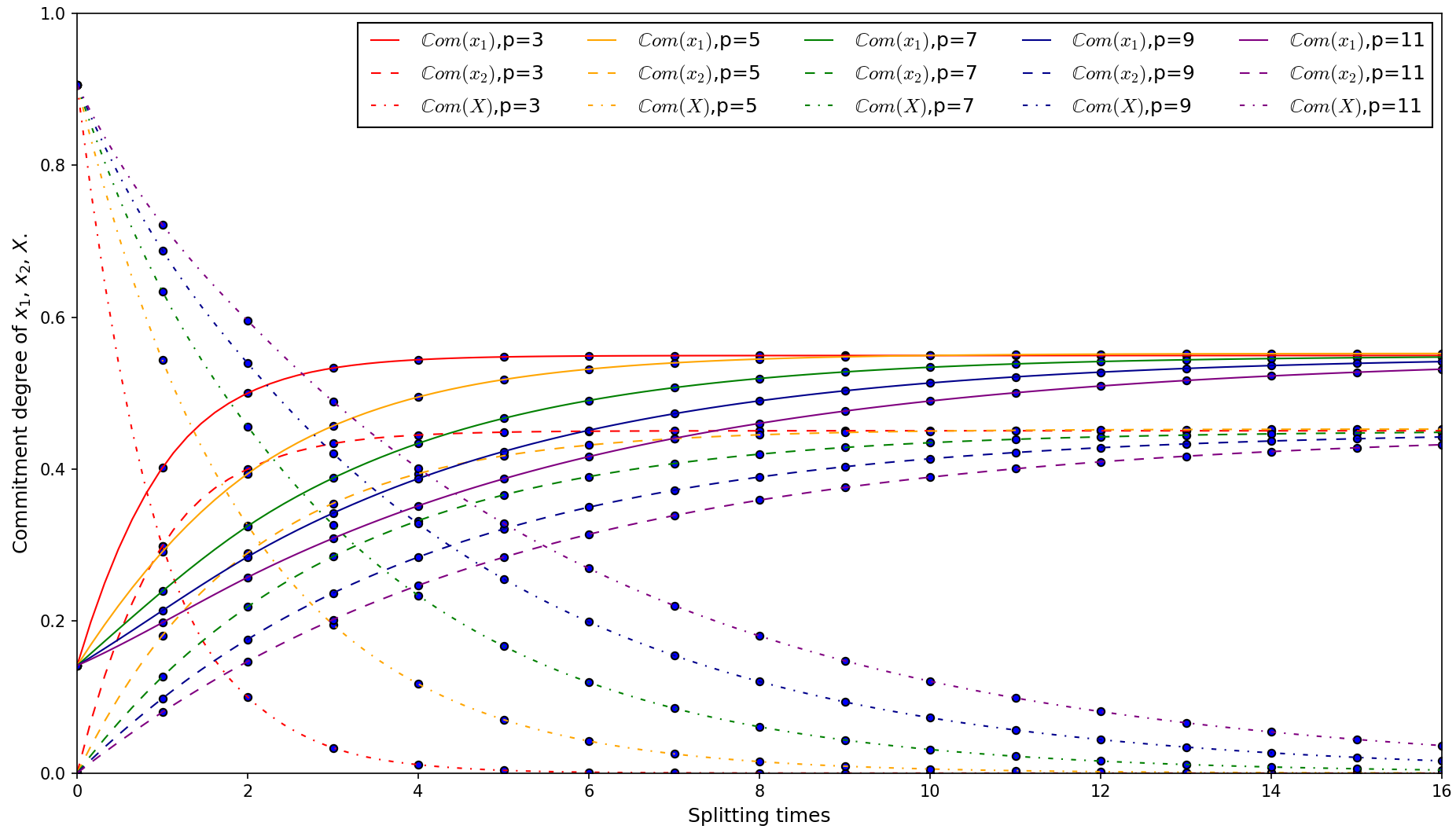
Figure 1: Regardless of the value of $p$, the final distribution of $\mathbb{C}om({{x}_{1}})$, $\mathbb{C}om({{x}_{2}})$ and $\mathbb{C}om({{X}})$ is stable and tends to the same value.

It is not difficult to understand the proposed CPBT generation process from Example III.1. For FoD with $n$ elements, give a CBBA $\mathbb{M}$. The production process of CPBT based on fractal is that the CBBA value of multi-element focal elements are evenly distributed to single element focal elements in a certain proportion in the process of time change, gradually reducing the influence of non-specificity until finally disappearing. Finally, the CBBA of Bayesian distribution is obtained.

An important feature of fractal is self-similarity. The proposed CPBT generation process is a self-similar iterative process. The fractal diagram of Example 1 is shown in Figure 2.

III-B Fractal-based complex belief entropy

Based on the above CPBT generation process, a new belief entropy called fractal-based complex belief (FCB) entropy is proposed to measure the uncertainty of CBBA. In the above two examples, when the parameters take different values, the size of multi-element focal element allocation is different. In FCB entropy, in order to better reflect the rationality of allocation, it is specified that the focal element is evenly allocated to each of its elements. The calculation diagram of FCB entropy is shown in Figure 3.

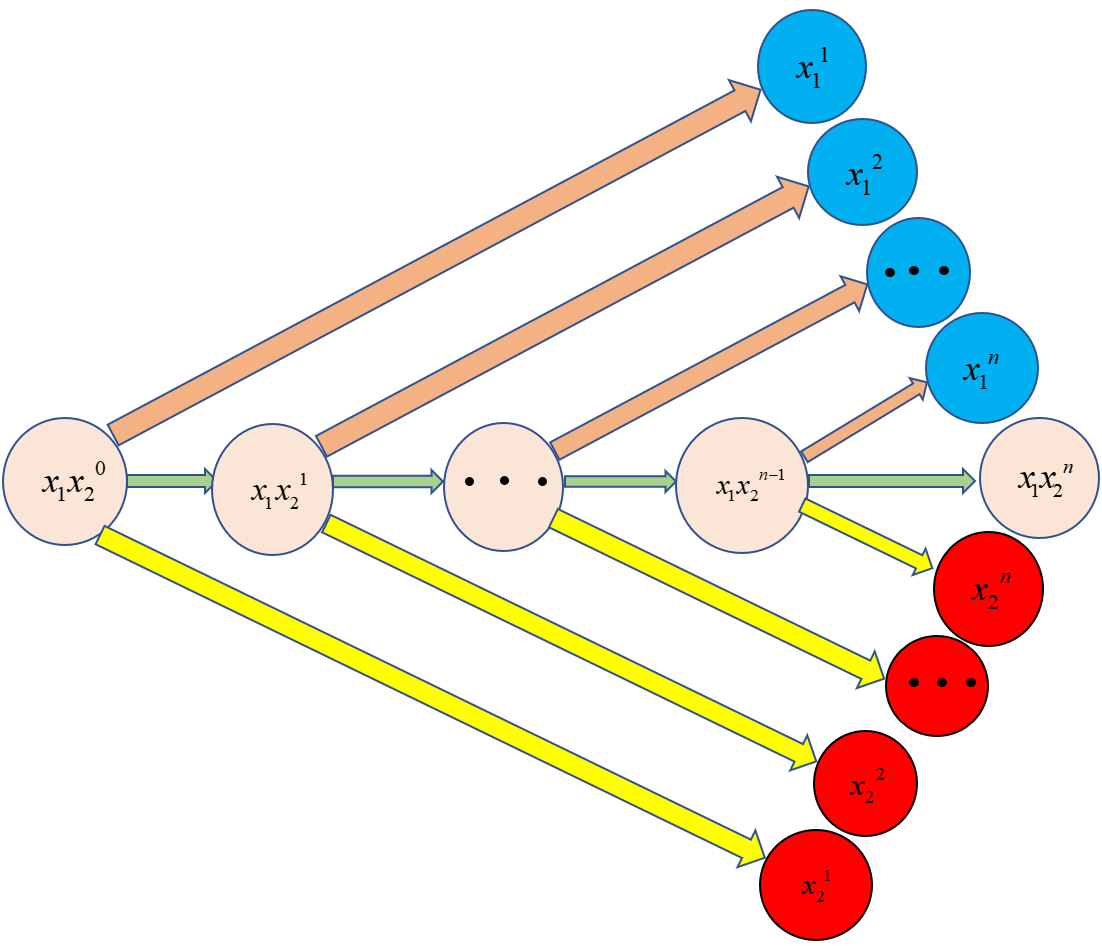
Figure 2: The process of $x_{1}$, $x_{2}$ allocation to singletons in Example 1 is self-similar.

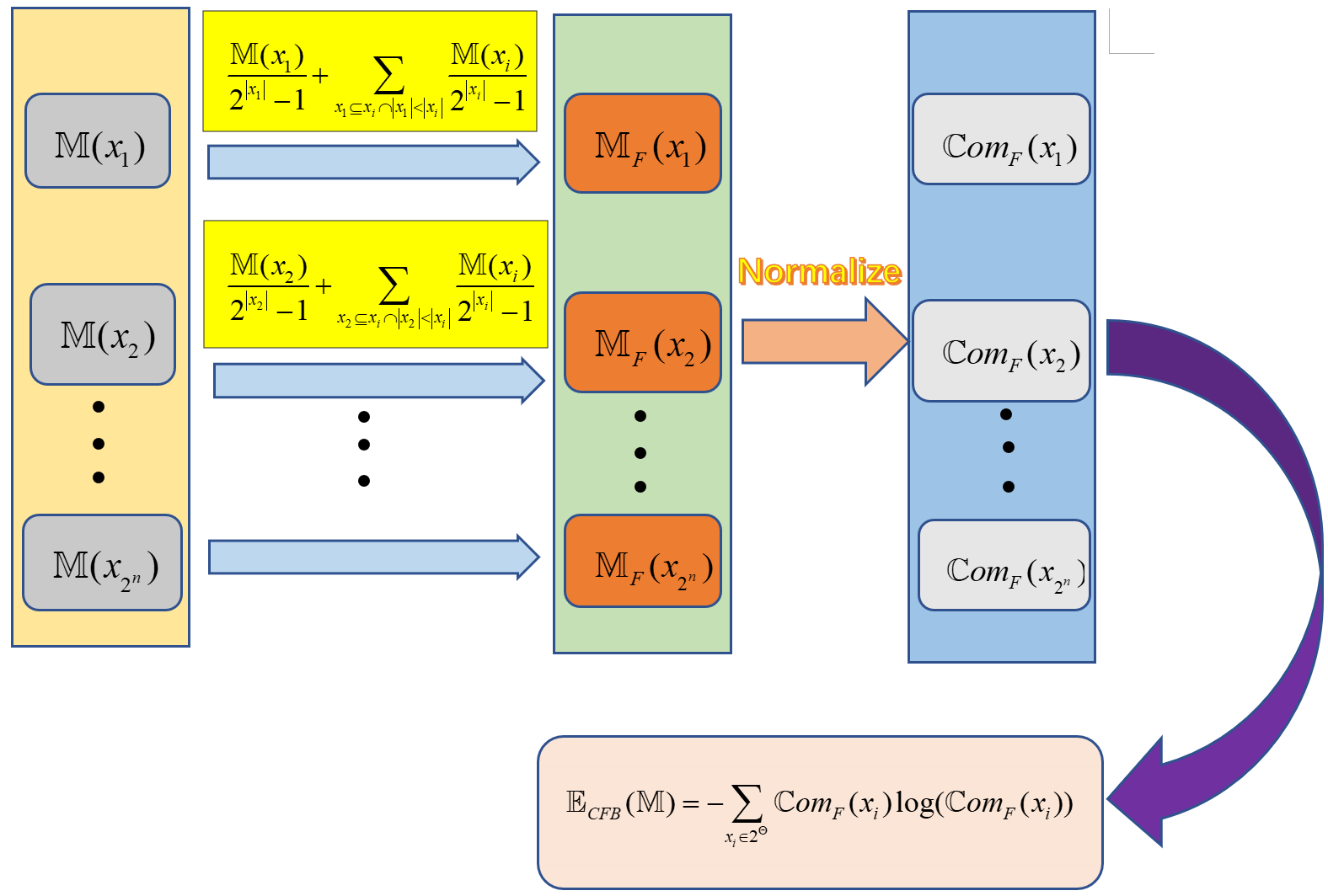
Figure 3: Flow chart of FCB entropy’s measurement.

Definition III.1.

(FCBBA). Given a FoD $\Theta=\{{{e}_{1}},{{e}_{2}},\cdots,{{e}_{n}}\}$ and its corresponding CBBA $\mathbb{M}$, For any ${{A}_{k}}$ belonging to ${{2}^{\Theta}}$, its CBBA after fractal is defined by

$$\small{{\mathbb{M}}_{F}}({{A}_{k}})=\frac{\mathbb{M}({{A}_{k}})}{{{2}^{\left|{{A}_{k}}\right|}}-1}+\sum\limits_{{{A}_{k}}\subseteq{{B}_{k}}\cap\left|{{A}_{k}}\right|<\left|{{B}_{k}}\right|}{\frac{\mathbb{M}({{B}_{k}})}{{{2}^{\left|{{B}_{k}}\right|}}-1}}.$$ (21)

The new set $2_{FB}^{\Theta}$ composed of ${{\mathbb{M}}_{F}}({{A}_{k}})=\frac{\mathbb{M}({{A}_{k}})}{{{2}^{\left|{{A}_{k}}\right|}}-1}+\sum\limits_{{{A}_{k}}\subseteq{{B}_{k}}\cap\left|{{A}_{k}}\right|<\left|{{B}_{k}}\right|}{\frac{\mathbb{M}({{B}_{k}})}{{{2}^{\left|{{B}_{k}}\right|}}-1}}$ is called fractal-based complex basic belief assignment (FCBBA).

Definition III.2.

(FCB entropy). Given a FoD $\Theta=\{{{e}_{1}},{{e}_{2}},\cdots,{{e}_{n}}\}$ and its corresponding FCBBA ${{\mathbb{M}}_{F}}({{A}_{k}})=\frac{\mathbb{M}({{A}_{k}})}{{{2}^{\left|{{A}_{k}}\right|}}-1}+\sum\limits_{{{A}_{k}}\subseteq{{B}_{k}}\cap\left|{{A}_{k}}\right|<\left|{{B}_{k}}\right|}{\frac{\mathbb{M}({{B}_{k}})}{{{2}^{\left|{{B}_{k}}\right|}}-1}}$, then the FCB entropy is defined by:

$${{\mathbb{E}}_{FCB}}(\mathbb{M}) =-\sum\limits_{{{A}_{k}}\in{{2}^{\Theta}}}{\mathbb{C}o{{m}_{F}}({{A}_{k}})\log(\mathbb{C}o{{m}_{F}}({{A}_{k}}))},$$ (22)

where $\mathbb{C}o{{m}_{F}}({{A}_{k}})$ represents the support degree for ${{A}_{k}}$ in $2_{FB}^{\Theta}$ and $\mathbb{C}o{{m}_{F}}({{A}_{k}})$ in the FCB entropy is defined by

$$\small\mathbb{C}o{{m}_{F}}({{A}_{k}})=\frac{\left|{{\mathbb{M}}_{F}}({{A}_{k}})\right|}{\sum\limits_{B\in\Theta}{\left|{{\mathbb{M}}_{F}}({{B}_{k}})\right|}},$$ (23)

where $\sum\limits_{B\in\Theta}{\left|{{\mathbb{M}}_{F}}({{B}_{k}})\right|}$ is used to normalize $\mathbb{C}o{{m}_{F}}({{A}_{k}})$, which ensures that the value of $\mathbb{C}o{{m}_{F}}({{A}_{k}})$ is between [0,1]. So $\mathbb{C}o{{m}_{F}}({{A}_{k}})$ also satisfies the following equation

$$\small\sum\limits_{{{A}_{k}}\in{{2}^{\Theta}}}{\mathbb{C}o{{m}_{F}}({{A}_{k}})}=1.$$ (24)

When substituting (23) into (22), (22) can be transformed into another form,

$$\small{{\mathbb{E}}_{FCB}}(\mathbb{M})=-\sum\limits_{{{A}_{k}}\in{{2}^{\Theta}}}{\frac{\left|{{\mathbb{M}}_{F}}({{A}_{k}})\right|}{\sum\limits_{B\in\Theta}{\left|{{\mathbb{M}}_{F}}({{B}_{k}})\right|}}\log\left(\frac{\left|{{\mathbb{M}}_{F}}({{A}_{k}})\right|}{\sum\limits_{B\in\Theta}{\left|{{\mathbb{M}}_{F}}({{B}_{k}})\right|}}\right)}.$$ (25)

The formula for calculating the modulus of the focal element in $\mathbb{C}o{{m}_{F}}({{A}_{k}})$ is defined as follows:

$$\left|{{\mathbb{M}}_{F}}({{A}_{k}})\right| =\left|\frac{\mathbb{M}({{A}_{k}})}{{{2}^{\left|{{A}_{k}}\right|}}-1}+\sum\limits_{{{A}_{k}}\subseteq{{B}_{k}}\cap\left|{{A}_{k}}\right|<\left|{{B}_{k}}\right|}{\frac{\mathbb{M}({{B}_{k}})}{{{2}^{\left|{{B}_{k}}\right|}}-1}}\right|$$ (26)

$$=\sqrt{{{\sum\limits_{{{C}_{k}}\in{{B}_{k}}}{\left|\frac{\mathbb{M}({{C}_{k}})}{{{2}^{\left|{{C}_{k}}\right|}}-1}\right|}}^{2}}+\sum\limits_{{{A}_{k}}\subseteq{{B}_{k}}\cap\left|{{A}_{k}}\right|<\left|{{B}_{k}}\right|}{IE({{B}_{k}})}}$$

where $IE({B}_{k})$ is the interference function in CET and in FCB entropy it is defined by

$$\underset{{B}_{k}\subseteq\Theta}{\mathop{IE({B}_{k})}} =\sum\limits_{{{X}_{i}}\subseteq{{B}_{k}},{{X}_{j}}\subseteq{{B}_{k}},{{X}_{i}}\neq{{X}_{j}}}{2\mathbf{m}({{X}_{i}})\mathbf{m}({{X}_{j}})\cos(\theta({{X}_{i}})-\theta({{X}_{j}}))}$$ (27)

$$={{\left|\sum\limits_{{{X}_{i}}\subseteq{B}_{k}}{\mathbb{M}({{X}_{i}})}\right|}^{2}}-\sum\limits_{{{X}_{i}}\subseteq{B}_{k}}{{{\mathbf{m}}^{2}}({{X}_{i}})}.$$

$\mathbb{M}({{X}_{i}})$ and $\mathbb{M}({{X}_{j}})$ have the same form as CBBA in CET

$$\small\mathbb{M}({{X}_{i}})=u+vi.$$ (28)

$\theta({{X}_{i}})$ can be calculated by the following formula

$$\small\theta\left({{X}_{i}}\right)=\left\{\begin{matrix}\arctan\left(\frac{v}{u}\right),&u>0\\ \frac{\pi}{2},&u=0,v>0\\ -\frac{\pi}{2},&u=0,v<0\\ \arctan\left(\frac{v}{u}\right)+\pi,&u<0,v\geq 0\\ \arctan\left(\frac{v}{u}\right)-\pi,&u<0,v<0\\ \end{matrix}\right.$$ (29)

After Euler transformation, $\mathbb{M}({{X}_{i}})$ and $\mathbb{M}({{X}_{j}})$ in $IE({B}_{k})$ can be expressed as

$$\small\mathbb{M}({{X}_{i}})=\mathbf{m}({{X}_{i}}){{e}^{i\theta({{X}_{i}})}},$$ (30)

$$\small\mathbb{M}({{X}_{j}})=\mathbf{m}({{X}_{j}}){{e}^{i\theta({{X}_{j}})}},$$ (31)

In the complex plane, the vector sum of $\mathbb{M}({{X}_{i}})$ and $\mathbb{M}({{X}_{j}})$ can be expressed by

$$\small\mathbb{M}({{X}_{i}})+\mathbb{M}({{X}_{j}})=\mathbf{m}({{X}_{i}}){{e}^{i\theta({{X}_{i}})}}+\mathbf{m}({{X}_{j}}){{e}^{i\theta({{X}_{j}})}}.$$ (32)

It can be calculated from cosine theorem that

$${{\left|\mathbf{m}({{X}_{i}}){{e}^{i\theta({{X}_{i}})}}+\mathbf{m}({{X}_{j}}){{e}^{i\theta({{X}_{j}})}}\right|}^{2}}$$ (33)

$$={{\left|\mathbf{m}({{X}_{i}}){{e}^{i\theta({{X}_{i}})}}\right|}^{2}}+{{\left|\mathbf{m}({{X}_{j}}){{e}^{i\theta({{X}_{j}})}}\right|}^{2}}+IE(X),$$

where $IE(X)=2\mathbf{m}({{X}_{i}})\mathbf{m}({{X}_{j}})\cos(\theta({{X}_{i}})-\theta({{X}_{j}}))$.

Through analysis, it can be seen that when $\left|X({{\theta}_{i}})-X({{\theta}_{j}})\right|\in[0,\frac{\pi}{2})\cup(\frac{3\pi}{2},2\pi]$, that is $\cos(X({{\theta}_{i}})-X({{\theta}_{j}}))>0$, $IE(X)>0$, which results in positive interference effect; when $\left|X({{\theta}_{i}})-X({{\theta}_{j}})\right|\in(\frac{\pi}{2},\frac{3\pi}{2})$, that is $\cos(X({{\theta}_{i}})-X({{\theta}_{j}}))<0$, $IE(X)<0$, which results in negative interference effect; when $\left|X({{\theta}_{i}})-X({{\theta}_{j}})\right|=\frac{\pi}{2}$ or $\left|X({{\theta}_{i}})-X({{\theta}_{j}})\right|=\frac{3\pi}{2}$, that is $\cos(X({{\theta}_{i}})-X({{\theta}_{j}}))=0$, $IE(X)=0$, which results in no interference effect. The results of the analysis are shown in the three subgraphs in Figure 4 below.

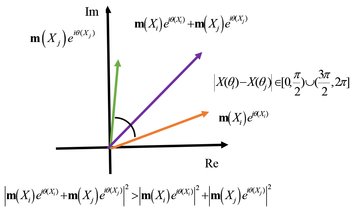
(a) Positive interference

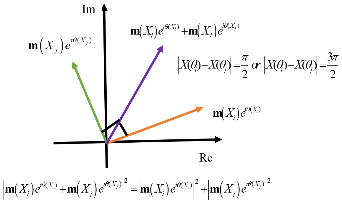
(b) Null interference

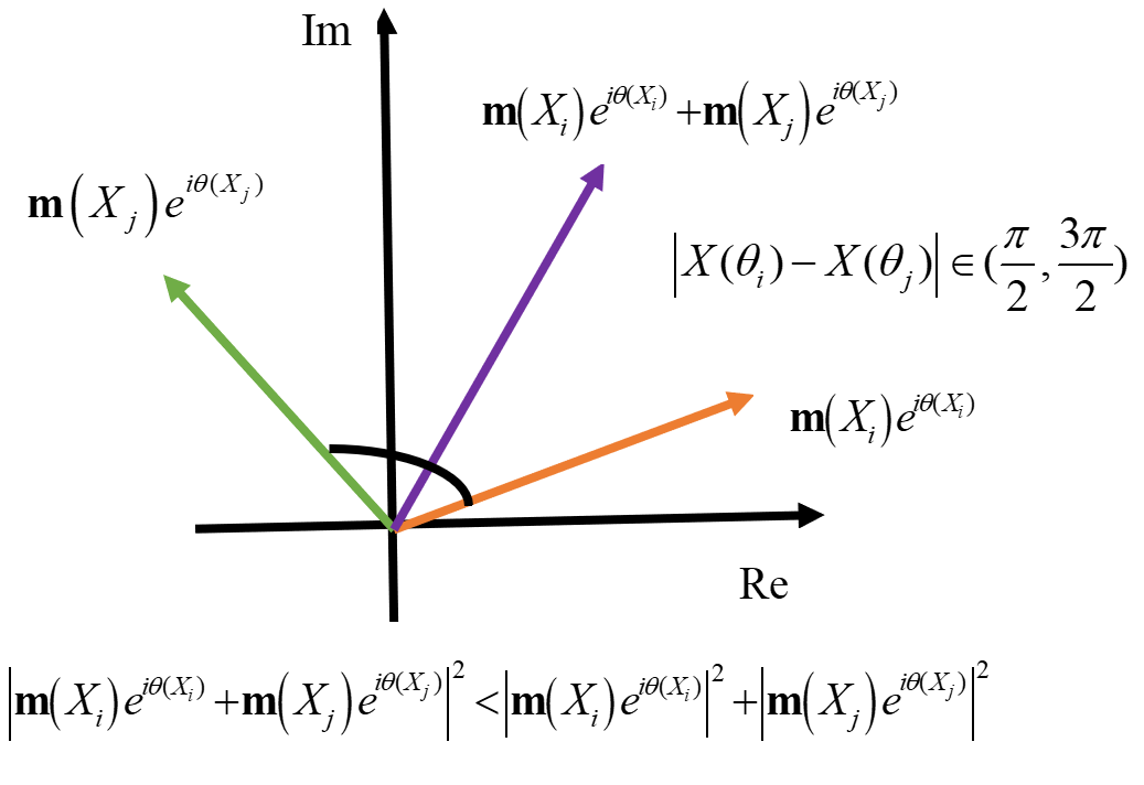
(c) Negative interference

Figure 4: Interference effect between two elements.

The existence of $IE({B}_{k})$ will have different impacts on $\mathbb{C}o{{m}_{F}}({{A}_{k}})$, mainly in the following three cases.

Case 1. For $\left|{{B}_{k}}\right|>\left|{{A}_{k}}\right|$, when $\mathbb{M}({{B}_{k}})$ is evenly distributed to the set $\mathbb{M}({{A}_{k}})$, its complex value and the required complex value tend to the same direction, resulting in a greater degree of support for ${{A}_{k}}$ than the normal state, making $\mathbb{C}o{{m}_{F}}({{A}_{k}})$ larger.

Case 2. For $\left|{{B}_{k}}\right|<\left|{{A}_{k}}\right|$, when $\mathbb{M}({{B}_{k}})$ is evenly distributed to the set $M({{A}_{k}})$, its complex value deviates from the direction of the required complex value of $\mathbb{M}({{A}_{k}})$, resulting in less support than the normal state, making $\mathbb{C}o{{m}_{F}}({{A}_{k}})$ smaller.

Case 3. For $\left|{{B}_{k}}\right|=\left|{{A}_{k}}\right|$, when $\mathbb{M}({{B}_{k}})$ is evenly distributed to the set $\mathbb{M}({{A}_{k}})$, its complex value is consistent with the direction of the required complex value of $\mathbb{M}({{A}_{k}})$, resulting in a support level equal to the normal state, which has no impact on $\mathbb{C}o{{m}_{F}}({{A}_{k}})$.

Axiom III.1.

When CBBA degenerates to BBA, FCB entropy degenerates to FB entropy, that is, In DSET, FCB entropy and FB entropy are equivalent.

Proof III.1.

When CBBA degenerates to BBA, the following formula can be obtained:

$$\small{{\mathbf{m}}_{F}}({{A}_{k}})=\frac{\mathbf{m}({{A}_{k}})}{{{2}^{\left|{{A}_{k}}\right|}}-1}+\sum\limits_{{{A}_{k}}\subseteq{{B}_{k}}\cap\left|{{A}_{k}}\right|<\left|{{B}_{k}}\right|}{\frac{\mathbf{m}({{B}_{k}})}{{{2}^{\left|{{B}_{k}}\right|}}-1}}.$$ (34)

Because BBA is defined in the real number field, there is no interference effect, namely, $\sum\limits_{{{A}_{k}}\subseteq{{B}_{k}}\cap\left|{{A}_{k}}\right|<\left|{{B}_{k}}\right|}{IE(B_{k})=0}$.

$$\small\left|{{\mathbf{m}}_{F}}({{A}_{k}})\right|={{\mathbf{m}}_{F}}({{A}_{k}}),$$ (35)

since the value range of BBA is [0,1],

$$\small\mathbb{C}o{{m}_{F}}({{A}_{k}})=\frac{\left|{{\mathbf{m}}_{F}}({{A}_{k}})\right|}{\sum\limits_{B\in\Theta}{\left|{{\mathbf{m}}_{F}}({{B}_{k}})\right|}}={{\mathbf{m}}_{F}}({{A}_{k}}).$$ (36)

Then simplify the FCB entropy to obtain

$${{\mathbb{E}}_{FCB}}(m)={{E}_{FB}}(m) =-\sum\limits_{{{A}_{k}}\in{{2}^{\Theta}}}{\mathbb{C}o{{m}_{F}}({{A}_{k}})\log(\mathbb{C}o{{m}_{F}}({{A}_{k}}))}$$ (37)

$$=-\sum\limits_{{{A}_{k}}\in{{2}^{\Theta}}}{{{m}_{F}}({{A}_{k}})\log({{m}_{F}}({{A}_{k}}))}.$$

Therefore, FCB entropy can be regarded as the generalization of FB entropy, which has better ability to process complex information than FB entropy.

III-C Maximum fractal-based complex belief entropy

The maximum entropy principle is a criterion for selecting the distribution of random variables that best conforms to the objective situation, also known as the maximum information principle. Generally, only one distribution has the maximum entropy. Choosing this distribution with maximum entropy as the distribution of the random variable is an effective criterion for decision analysis. Therefore, the derivation of the maximum FCB entropy model is very important. The definition of maximum FCB entropy is as follows.

Definition III.3.

(Maximum FCB entropy). Given a FoD $\Theta=\{{{e}_{1}},{{e}_{2}},\cdots,{{e}_{n}}\}$ and the CBBA $\mathbb{M}$ in it, the maximum FCB entropy is

$$\small\mathbb{E}_{FCB}^{\max}(\mathbb{M})=\log({{2}^{\left|\Theta\right|}}-1)=\log({{2}^{n}}-1),$$ (38)

when $\mathbb{C}o{{m}_{F}}({{A}_{k}})=\frac{1}{{{2}^{\left|\Theta\right|}}-1}$.

Proof III.2.

First, FCB entropy is expressed as a function

$$\small{{f}_{FCB}}({{A}_{1}},\cdots,{{A}_{{{2}^{\left|\Theta\right|}}-1}})=-\sum\limits_{{{A}_{k}}\in{{2}^{\Theta}}}{\mathbb{C}o{{m}_{F}}({{A}_{k}})\log(\mathbb{C}o{{m}_{F}}({{A}_{k}}))},$$ (39)

according to (24), that is, $\sum\limits_{{{A}_{k}}\in{{2}^{\Theta}}}{\mathbb{C}o{{m}_{F}}({{A}_{k}})}=1$. Therefore, the Lagrange function can be constructed as

$${{\mathbb{F}}_{FCB}}({{A}_{1}},{{A}_{2}},\cdots,{{A}_{{{2}^{\left|\Theta\right|}}-1}},\lambda) ={{f}_{FCB}}({{A}_{1}},{{A}_{2}},\cdots,{{A}_{{{2}^{\left|\Theta\right|}}-1}})$$ (40)

$$+\lambda(\sum\limits_{{{A}_{k}}\in{{2}^{\Theta}}}{\mathbb{C}o{{m}_{F}}({{A}_{k}})}-1),$$

then calculate the first partial derivative of ${{\mathbb{F}}_{FCB}}({{A}_{1}},{{A}_{2}},\cdots,{{A}_{{{2}^{\left|\Theta\right|}}-1}})$. For all $\mathbb{C}o{{m}_{F}}({{A}_{k}})$,

$$\small\log(\mathbb{C}o{{m}_{F}}({{A}_{k}}))=\lambda-\frac{1}{\ln a}=k,$$ (41)

then according to (24),

$$\small\sum\limits_{{{A}_{k}}\in{{2}^{\Theta}}}{\mathbb{C}o{{m}_{F}}({{A}_{k}})}=({{2}^{\left|\Theta\right|}}-1)\mathbb{C}o{{m}_{F}}({{A}_{k}})=1,$$ (42)

so when $\mathbb{C}o{{m}_{F}}({{A}_{k}})=\frac{1}{({{2}^{\left|\Theta\right|}}-1)}$, FCB entropy reaches its maximum,

$$\small\mathbb{E}_{CFB}^{\max}(\mathbb{M})=-\sum\limits_{{{A}_{k}}\in{{2}^{\Theta}}}{\frac{1}{({{2}^{\left|\Theta\right|}}-1)}\log\frac{1}{({{2}^{\left|\Theta\right|}}-1)}}=\log({{2}^{\left|\Theta\right|}}-1).$$ (43)

FB entropy is a generalization of Shannon entropy. Its maximum entropy model is similar to Shannon entropy, and can also deal with decision-making problems in the objective world. As the generalization of FB entropy, the maximum entropy model of FCB entropy has the physical meaning of FB entropy and has more advantages.

IV The properties of the proposed FCB entropy

For the total uncertainty measurement of BBA, different methods generally have 10 properties, which are often used for the analysis of uncertain methods. For the analysis of FCB entropy, the 10 properties have been extended to CET to measure the feasibility and applicability of FCB entropy. The properties of some uncertain methods are summarized in Table I.

TABLE I: Summary of properties of some entropies.

	Properties
Measures	Probabilistic consistency	Set consistency	Additivity	Subadditivity	Maximum entropy
Hartley Entropy [63]	✗	✓	✓	✓	✓
Pal et al.’s entropy [37]	✓	✓	✓	✗	✗
Zhou et al.’s measure [64]	✓	✗	✓	✗	✓
Deng entropy [35]	✓	✗	✗	✗	✓
JS entropy [39]	✓	✓	✓	✗	✓
FB entropy [60]	✓	✗	✓	✓	✓
FCB entropy	✓	✗	✓	✓	✓

Property IV.1 (Probabilistic consistency).

When all focal elements are singletons, the distribution of mass function is similar to Bayesian distribution, and the total uncertainty measurement should be degenerated to Shannon entropy.

For FCB entropy, $\forall\left|{{A}_{i}}\right|>1,\mathbb{M}({{A}_{i}})=0$,$\left|{{\mathbb{M}}_{F}}({{A}_{i}})\right|=\left|\frac{\mathbb{M}({{A}_{i}})}{{{2}^{\left|{{A}_{i}}\right|}}-1}\right|$.

Case 1. when CBBA degenerates BBA and according to Axiom III.1, FCB entropy is degenerated to FB entropy. And the BBA in FoD $\Theta=\{{{e}_{1}},{{e}_{2}},\cdots,{{e}_{n}}\}$ satisfies $\sum\limits_{i=1}^{n}{m({{e}_{i}})}=1$, substitute it into (23):

$${{\mathbb{E}}_{FCB}}(m) =-\sum\limits_{i=1}^{n}{m({{e}_{i}})\log(m({{e}_{i}}))}$$ (44)

$$={{E}_{FB}}(m)={{E}_{s}}(m).$$

It is obvious that it satisfies Property IV.1.

Case 2. When FCB entropy is expressed in the form of CBBA, its probability consistency cannot be judged in the usual form. Expand it to use $\mathbb{C}om({{A}_{i}})$ to express the probability of focal element ${{A}_{i}}$. The CBBA in FoD $\Theta=\{{{e}_{1}},{{e}_{2}},\cdots,{{e}_{n}}\}$ satisfies $\sum\limits_{i=1}^{n}{\mathbb{M}({{e}_{i}})}=1$ and $\sum\limits_{i=1}^{n}{\mathbb{C}o{{m}_{F}}({{e}_{i}})}=1$, then substitute it into (23):

$${{\mathbb{E}}_{FCB}}(\mathbb{M}) =-\sum\limits_{i=1}^{n}{\mathbb{C}o{{m}_{F}}({{e}_{i}})\log(\mathbb{C}o{{m}_{F}}({{e}_{i}}))}$$ (45)

$$=-\sum\limits_{i=1}^{n}{\mathbb{C}om({{e}_{i}})\log(\mathbb{C}om({{e}_{i}}))}.$$

In CET, $\mathbb{C}om({{e}_{i}})$ represents the degree of support for a focal element ${{e}_{i}}$, which is similar to the role of probability in probability theory. The simplified FCB entropy has the same form as Shannon entropy, and is similar to the information it expresses. The generalized probability consistency of FCB entropy in the complex number field can also be satisfied.

Property IV.2 (Set correlation).

The number of elements in the focal element will also affect the information modeling when the complex mass function is allocated. The traditional set consistency is controversial, but it provides a new perspective for the study of the set-related properties of FCB entropy.

Explanation: Hartley’s information formula measures the amount of information in probability theory, while FCB entropy measures the uncertainty in FoD. In the case of the same dimension, evidence theory can express more information than probability theory. For a FoD with $n$ elements, the framework of evidence theory contains ${{2}^{n}}$ focal elements, while probability theory only contains $n$ elements. Therefore, it is reasonable that the maximum value of FCB entropy is greater than the maximum value of Shannon entropy. For some commonly used entropies, their maximum entropies are summarized in Table II. The maximum value of different entropy changes with the number of elements as shown in Figure 5.

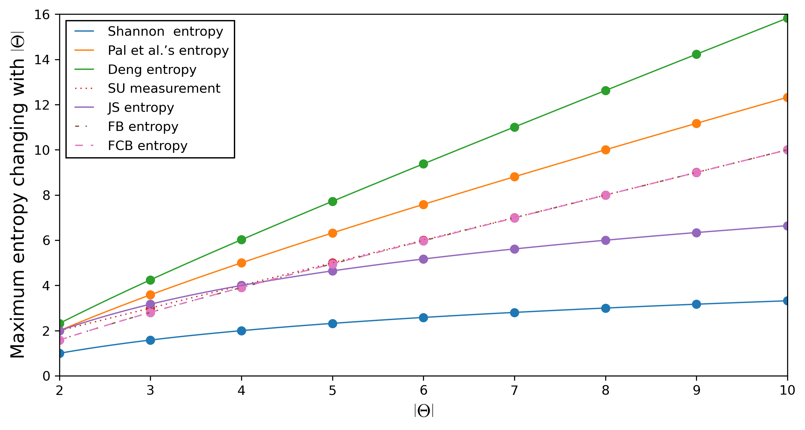
Figure 5: As the number of elements in FoD increases, the maximum value of most entropies is greater than the maximum value of Shannon entropy.

TABLE II: Summary of maximum of some entropies.

	Methods
	Shannon entropy	Pal et al.’s entropy [37]	Deng entropy [35]	SU measurement
Maximum	$\log\left(\left|\Theta\right|\right)$	$\log\left(\left|\Theta\right|\cdot{{2}^{\left|\Theta\right|-1}}\right)$	$\log\left({{3}^{\left|\Theta\right|}}-{{2}^{\left|\Theta\right|}}\right)$	$\left|\Theta\right|$
	JS entropy [39]	FB entropy [60]	FCB entropy
Maximum	$2\log\left(\left|\Theta\right|\right)$	$\log({{2}^{\left|\Theta\right|}}-1)$	$\log({{2}^{\left|\Theta\right|}}-1)$

Property IV.3 (Range).

Given a FoD $\Theta=\{{{e}_{1}},{{e}_{2}},\cdots,{{e}_{n}}\}$, the range of the total uncertainty measurements should be in $[0,\log\left|\Theta\right|]$.

Proof IV.1.

When there exists a elemnt in the FoD satisfying $\mathbb{M}({{e}_{i}})=1$, the minimum of FCB entropy is $\mathbb{E}_{FCB}^{\min}(\mathbb{M})=0$. In Definition III.3, the maximum of FCB entropy is defined as $\mathbb{E}_{FCB}^{\max}(\mathbb{M})=\log({{2}^{\left|\Theta\right|}}-1)=\log({{2}^{n}}-1)$. Therefore, the range of FCB entropy is $[0,\log({{2}^{n}}-1)]$. So FCB entropy doesn’t satisfy Property IV.3.

Property IV.4 (Monotonicity).

Monotonicity means that in evidence theory, when information is significantly reduced (uncertainty increases), the measurement method of total uncertainty should not reduce the uncertainty.

Specifically, in DSET let two CBBAs ${{\mathbb{M}}_{1}}$ and ${{\mathbb{M}}_{2}}$ be defined on a FoD $\Theta=\{{{e}_{1}},{{e}_{2}},\cdots,{{e}_{n}}\}$. For any focal element ${{P}_{i}}\subseteq\Theta$ satisfying

$$\small GBe{{l}_{1}}({{P}_{i}})\geq GBe{{l}_{2}}({{P}_{i}}),$$ (46)

it must satisfy the following relationship:

$$\small{{\mathbb{E}}_{FCB}}({{\mathbb{M}}_{1}})\leq{{\mathbb{E}}_{FCB}}({{\mathbb{M}}_{2}}).$$ (47)

Proof IV.2.

Negation is a good way to analyze problems in evidence theory. Considering events from the negative side, some problems that cannot be concluded from the positive side can be dealt with. As the number of negative iterations increases, the amount of information in evidence theory decreases and the uncertainty increases. In this paper, the negative idea is used to prove the monotonicity of FCB entropy.

Case 1. When CBBA is defined on the complex plane. Compared with the traditional entropy model, FCB entropy is used to measure the uncertainty of CBBA, and can deal with information in complex form. The monotonicity is verified by negative thinking. In CET, a new CBBA exponential negation method was proposed [55]. It provides a method to verify the monotonicity of FCB entropy. Consider a FoD $\Theta=\{{{e}_{1}},{{e}_{2}}\}$, select the initial value that is easy to calculate. And after 10 negative iterations, the results of CBBA in CET changing with the number of negations are shown in Table III. The calculation results of FCB entropy are shown in Table IV. It can be seen from Table IV that FCB entropy increases with the number of negation. So when FCB entropy is used on CBBA, it satisfies monotonicity.

TABLE III: CBBA changing with the number of negative iterations.

	CBBA
Times	$\mathbb{M}(e_{1})$	$\mathbb{M}(e_{2})$	$\mathbb{M}(\Theta)$
0	0.200+0.300i	0.500-0.100i	0.300-0.200i
1	0.211+0.050i	0.289-0.050i	0.500
2	0.240+0.012i	0.260-0.012i	0.500
3	0.248+0.003i	0.252-0.003i	0.500
4	0.249+0.001i	0.251-0.001i	0.500
5	0.250+0.001i	0.250-0.001i	0.500
6	0.250+0.000i	0.250-0.000i	0.500
7	0.250+0.000i	0.250-0.000i	0.500
8	0.250+0.000i	0.250-0.000i	0.500
9	0.250+0.000i	0.250-0.000i	0.500
10	0.250+0.000i	0.250-0.000i	0.500

TABLE IV: Results of each iteration of FCB entropy.

	Times
Measures	0	1	2	3	4	5	6	7	8	9	10
FCB entropy	1.3458	1.4633	1.4734	1.4834	1.4834	1.4834	1.4834	1.4834	1.4834	1.4834	1.4834

TABLE V: BBA changing with the number of negative iterations.

	Times
BBA	0	1	2	3	4	5	6	7	8	9	10
$m(e_{1})$	0.3333	0.1667	0.0833	0.0417	0.0208	0.0104	0.0052	0.0026	0.0013	0.0001	0.0000
$m({e}_{2})$	0.3333	0.1667	0.0833	0.0417	0.0208	0.0104	0.0052	0.0026	0.0013	0.0001	0.0000
$m(\Theta)$	0.3333	0.6667	0.8333	0.9167	0.9583	0.9781	0.9896	0.9948	0.9974	0.9998	1.0000

Case 2. According to Axiom III.1, as a generalization of FB entropy, when CBBA degenerates to BBA, FCB entropy degenerates into FB entropy. Luo proposed a negative method of BBA. The negative direction is the direction of neglect. Similar to the process in Case 1. Consider a FoD $\Theta=\{{{e}_{1}},{{e}_{2}}\}$, select the initial value that is easy to calculate. And after 10 negative iterations, the results of BBA in DSET changing with the number of negations are shown in the Table V. The calculation results of entropies are shown in Table VI. In the meantime, the change trend of FCB entropy and other previous entropies in evidence theroy with the number of iterations are shown in Figure 6. According to Figure 6, it’s clear to see that FB entropy [60] and FCB entropy increase with the number of iterations increasing, while Deng entropy [35], Pal et al.s’ entropy [37], Zhou et al.’s entropy [64] and Cui et al.s’ entropy [62] first increase and then decrease with the number of iterations increasing. That is, FB entropy and FCB entropy meet the requirements of monotonicity, while Deng entropy, Pal et al.s’ entropy, Zhou et al.’s entropy and Cui et al.s’ entropy does not meet the requirements of monotonicity.

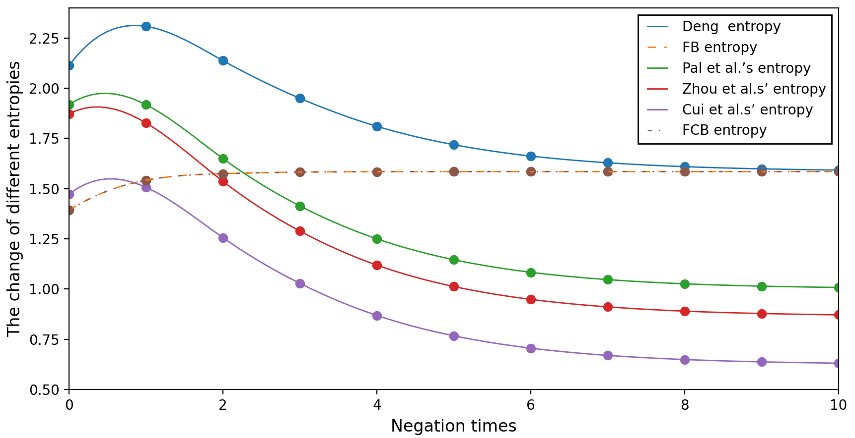
Figure 6: The change trend of different entropies with the increase of negation times.

TABLE VI: Results of each iteration of different entropies.

	Times
Measures	0	1	2	3	4	5	6	7	8	9	10
Deng entropy [35]	2.1133	2.3083	2.1375	1.9500	1.8105	1.7189	1.6624	1.6289	1.6095	1.5986	1.5924
FB entropy [60]	1.3921	1.5420	1.5746	1.5824	1.5843	1.5848	1.5849	1.5850	1.5850	1.5850	1.5850
Pal et al.s’ entropy [37]	1.9183	1.9182	1.6500	1.4138	1.2500	1.1461	1.0835	1.0470	1.0261	1.0144	1.0078
Zhou et al.’s entropy [64]	1.8728	1.8274	1.5364	1.2888	1.1192	1.0126	0.9486	0.9113	0.8900	0.8782	0.8715
Cui et al.s’ entropy [62]	1.4721	1.5068	1.2558	1.0283	0.8687	0.7671	0.7056	0.6696	0.6490	0.6374	0.6309
FCB entropy	1.3921	1.5420	1.5746	1.5824	1.5843	1.5848	1.5849	1.5850	1.5850	1.5850	1.5850

Combining the above two cases, it can be verified that FCB entropy satisfies monotonicity.

Property IV.5 (Additivity).

Given two independent FoD $\Gamma$ and $\Upsilon$, two CBBAs are defined on the two FoDs, respectively. Let $\Psi=\Gamma\times\Upsilon$ be a joint FoD. Then the total uncertainty measurement should satisfy

$$\small{{\mathbb{E}}_{FCB}}({{\mathbb{M}}_{\Psi}})={{\mathbb{E}}_{FCB}}({{\mathbb{M}}_{\Gamma}})+{{\mathbb{E}}_{FCB}}({{\mathbb{M}}_{\Upsilon}}).$$ (48)

For BBA, there are two different definitions of joint BBA depending on whether $m(\varnothing)=0$. In this paper, assuming that CBBA is normalized, the framework of joint CBBA is defined as $\Gamma\times\Upsilon=({{2}^{\left|\Gamma\right|}}-1)({{2}^{\left|\Upsilon\right|}}-1)$.

According to the above definition, the number of complex quality functions of $\Psi$ is less than its power set. For FCB entropy, the average distribution of multifocal elements to power sets should be changed to the number of subsets assigned to this frame. Joint CBBA ${{\mathbb{M}}^{\Psi}}$ and joint FCBBA $\mathbb{M}_{F}^{\Psi}$ are defined by

$${{\mathbb{M}}^{\Psi}}({{\psi}_{ij}})=\mathbb{M}({{\tau}_{i}})\times\mathbb{M}({{\gamma}_{j}}),$$ (49)

$${{\mathbb{M}}^{\Psi}}({{\psi}_{ij}}{{\psi}_{im}})=\mathbb{M}({{\tau}_{i}})\times\mathbb{M}({{\gamma}_{j}}{{\gamma}_{m}}),$$

$${{\mathbb{M}}^{\Psi}}({{\psi}_{ij}}{{\psi}_{im}}{{\psi}_{nj}}{{\psi}_{nm}})=\mathbb{M}({{\tau}_{i}}{{\tau}_{n}})\times\mathbb{M}({{\gamma}_{j}}{{\gamma}_{m}}),$$

$$\forall{{A}_{i}}\in{{2}^{\left|\Psi\right|}},\mathbb{M}_{F}^{\Psi}({{A}_{i}})={{\mathbb{M}}^{\Psi}}({{A}_{i}})+\sum\limits_{{{A}_{i}}\subseteq{{D}_{i}};{{B}_{i}}\times{{C}_{i}}={{D}_{i}}}{\frac{{{\mathbb{M}}^{\Psi}}({{D}_{i}})}{S\left({{B}_{i}},{{C}_{i}}\right)}},$$

where $S\left({{B}_{i}},{{C}_{i}}\right)=({{2}^{\left|{{B}_{i}}\right|}}-1)({{2}^{\left|{{C}_{i}}\right|}}-1)$.

Proof IV.3.

Given $\psi\in{{2}^{\left|\Psi\right|}}$, $\tau\in{{2}^{\left|\Gamma\right|}}$ and $\gamma\in{{2}^{\left|\Upsilon\right|}}$, and the relationship of the three FoDs is $\Psi=\Gamma\times\Upsilon$. According to Definition III.1, the following equation is derived

$$\mathbb{M}_{F}^{\Psi}(\psi) =\mathbb{M}(\tau)\times\mathbb{M}(\gamma)+\sum\limits_{{{A}_{i}}\subseteq{{D}_{i}};{{B}_{i}}\times{{C}_{i}}={{D}_{i}}}{\frac{\mathbb{M}({{B}_{i}})\times\mathbb{M}({{C}_{i}})}{S\left({{B}_{i}},{{C}_{i}}\right)}}$$ (50)

$$=\mathbb{M}_{F}^{\Gamma}(\tau)\times\mathbb{M}_{F}^{\Upsilon}(\gamma)$$

then calculate the modulus of $M_{F}^{\Psi}(\psi)$ to obtain the following equation

$$\small\left|\mathbb{M}_{F}^{\Psi}(\psi)\right|=\left|\mathbb{M}_{F}^{\Gamma}(\tau)\right|\times\left|\mathbb{M}_{F}^{\Upsilon}(\gamma)\right|,$$ (51)

next, normalize the obtained FCBBA modulus

$$\small\mathbb{C}o{{m}_{F}}(\psi)=\frac{\left|\mathbb{M}_{F}^{\Gamma}(\tau)\right|\times\left|\mathbb{M}_{F}^{\Upsilon}(\gamma)\right|}{\sum\limits_{{{\tau}_{i}}\in{{2}^{\Gamma}};{{\gamma}_{i}}\in{{2}^{\Upsilon}}}{\left|\mathbb{M}_{F}^{\Gamma}({{\tau}_{i}})\right|\times\left|\mathbb{M}_{F}^{\Upsilon}({{\gamma}_{i}})\right|}}.\\$$ (52)

It is proved that the joint CBBA and FCBBA are continuous in the framework. In addition, it is also known that Shannon entropy is additive, and FCB entropy is similar to Shannon entropy. It is easy to prove that FCB entropy is additive. An example is given below to verify that FCB entropy satisfies additivity.

Example IV.1.

Given two independent FoD $X=\{{{x}_{1}},{{x}_{2}}\}$ and $Y=\{{{y}_{1}},{{y}_{2}}\}$, two CBBAs are defined on the two FoDs, respectively. Let $Z=X\times Y$ be a joint FoD. And the complex mass functions are

$${{\mathbb{M}}^{X}}: {{\mathbb{M}}^{X}}({{x}_{1}})=0.2+0.1i,{{\mathbb{M}}^{X}}({{x}_{2}})=0.5+0.1i,$$

$${{\mathbb{M}}^{X}}({{x}_{1}},{{x}_{2}})=0.3-0.2i,$$

$${{\mathbb{M}}^{Y}}: {{\mathbb{M}}^{Y}}({{y}_{1}})=0.3+0.2i,{{\mathbb{M}}^{Y}}({{y}_{2}})=0.2+0.1i,$$

$${{\mathbb{M}}^{Y}}({{y}_{1}},{{y}_{2}})=0.5-0.3i.$$

Using the normalized $\mathbb{C}o{{m}_{F}}$ to calculate the FCB entropy, it can be obtained that

$${{\mathbb{E}}_{FCB}}({{\mathbb{M}}_{Z}})=2.8317={{\mathbb{E}}_{FCB}}({{\mathbb{M}}_{X}})+{{\mathbb{E}}_{FCB}}({{\mathbb{M}}_{Y}}),$$

which indicates that FCB entropy satisfies additivity.

Property IV.6 (Subadditivity).

Given two independent FoDs $\Gamma$ and $\Upsilon$, two CBBAs are defined on the two FoDs, respectively. Let $\Psi=\Gamma\times\Upsilon$ be a joint FoD. Then the total uncertainty measurement should satisfy

$$\small{{\mathbb{E}}_{FCB}}({{\mathbb{M}}_{\Psi}})\leq{{\mathbb{E}}_{FCB}}({{\mathbb{M}}_{\Gamma}})+{{\mathbb{E}}_{FCB}}({{\mathbb{M}}_{\Upsilon}}).$$ (53)

Proof IV.4.

Whether the two FoDs $\Gamma$ and $\Upsilon$ are independent will have an impact on the entropy of the combined FoD $\Psi$, which is mainly divided into the following two cases.

Case 1. If CBBAs in $\Gamma$ and $\Upsilon$ are independent of each other, it can be known from Property 5 that ${{\mathbb{E}}_{FCB}}({{\mathbb{M}}_{\Psi}})={{\mathbb{E}}_{FCB}}({{\mathbb{M}}_{\Gamma}})+{{\mathbb{E}}_{FCB}}({{\mathbb{M}}_{\Upsilon}})$.

Case 2. If CBBAs in $\Gamma$ and $\Upsilon$ are not independent of each other, when the two CBBAs are jointed, there will be some overlapping information, resulting in reduced uncertainty, namely ${{\mathbb{E}}_{FCB}}({{\mathbb{M}}_{\Psi}})<{{\mathbb{E}}_{FCB}}({{\mathbb{M}}_{\Gamma}})+{{\mathbb{E}}_{FCB}}({{\mathbb{M}}_{\Upsilon}})$.

Combining the above two cases, it can be concluded that FCB entropy satisfies the subadditivity.

Property IV.7 (Time complexity).

Let a CBBA $\mathbb{M}$ be defined on a FoD $\Theta=\{{{e}_{1}},{{e}_{2}},\cdots,{{e}_{n}}\}$ which contains $n$ elements. The measurement of FCB entropy can be divided into four steps. The total time complexity of each step and the algorithm is summarized in Table VII.

[b] Steps Time complexity Description Step 1 $O(n{{2}^{n}})$ Calculate FCBBA based on CBBA Step 2 $O({{2}^{n}})$ Calculate the modulus of FCBBA. Step 3 $O({{2}^{n}})$ Calculate $\mathbb{C}o{{m}_{F}}$ of each focal element. Step 4 $O({{2}^{n}})$ Finally, calculate FCB entropy. Step 1-4 $O(n{{2}^{n}})$ Time complexity.

TABLE VII: Time complexity of each step in the propoed FCB entropy

• Explanation of notations in the table:

• $n$: The number of baic event in the frame of discernment $\Theta$.

• $O(f\left(n\right))$: The maximum time complexity.

According to Table VII, it can be seen that the computational complexity of FCB entropy is similar to that of FB entropy [60] and JS entropy [39], and the computational complexity of some methods is higher than that of FCB entropy. Therefore, the computational complexity of FCB entropy is still within an acceptable range.

Property IV.8 (Discord and non-specificity).

For a total uncertain measurement method, it should be able to be divided into two parts to measure discord and non-specificity.

Definition IV.1.

(FCB entropy’s discord). Given a FoD $\Theta=\{{{e}_{1}},{{e}_{2}},\cdots,{{e}_{n}}\}$ and a CBBA $\mathbb{M}$ is defined in it, then the FCB entropy’s discord part is defined by

$$\small\mathbb{E}_{FCB}^{\mathcal{D}}(\mathbb{M})=-\sum\limits_{i=1}^{n}{\mathbb{C}omCBet({{e}_{i}})\log\left(\mathbb{C}omCBet({{e}_{i}})\right)},$$ (54)

in which

$$\small\mathbb{C}omCBet({{e}_{i}})=\frac{\left|CBet({{e}_{i}})\right|}{\sum\limits_{i=1}^{n}{\left|CBet({{e}_{i}})\right|}},$$ (55)

where $\sum\limits_{i=1}^{n}{\left|CBet({{e}_{i}})\right|}$ is used to normalize $\left|CBet({{e}_{i}})\right|$ and ensures the range of $\mathbb{C}omCBet({{e}_{i}})$ is in $[0,1]$.

Definition IV.2.

(FCB entropy’s non-specificity). Given a FoD $\Theta=\{{{e}_{1}}$, ${{e}_{2}}$, $\cdots$,${{e}_{n}}\}$ and a CBBA $\mathbb{M}$ is defined in it. Then the FCB entropy’s non-specificity part is defined by

$$\mathbb{E}_{FCB}^{\mathcal{N}}(\mathbb{M})= {{\mathbb{E}}_{FCB}}(\mathbb{M})-\mathbb{E}_{FCB}^{\mathcal{D}}(\mathbb{M})$$ (56)

$$= \sum\limits_{i=1}^{n}{\mathbb{C}omCBet({{e}_{i}})\log\left(\mathbb{C}omCBet({{e}_{i}})\right)}$$

$$-\sum\limits_{{{A}_{i}}\in{{2}^{\Theta}}}{\mathbb{C}o{{m}_{F}}({{A}_{i}})\log(\mathbb{C}o{{m}_{F}}({{A}_{i}}))}$$

Among the existing methods, there are entropies that can be directly decomposed into discord and non-specificity from the formula, such as Deng entropy and JS entropy. However, similar to FB entropy, the measurement of FCB entropy on discord and non-specificity is not directly obtained from the formula. FCB entropy originates from the production process of CPBT. When CBBA is converted to probability through CPBT, there is only uncertainty caused by discord in the framework. Therefore, the definitions of discord and non-specificity in FCB entropy are as above.

In Definition IV.1, $\mathbb{E}_{FCB}^{\mathcal{D}}(\mathbb{M})$ represents the uncertainty caused by singletons, excluding the uncertainty caused by set allocation in evidence theory. So it is reasonable to represent the discord in FCB entropy. Total uncertainty minus the uncertainty caused by discord is the uncertainty caused by non-specificity. Therefore, FCB entropy satisfies Property IV.8.

An example is given below to show the relationship between the discord and non-specificity of FCB entropy.

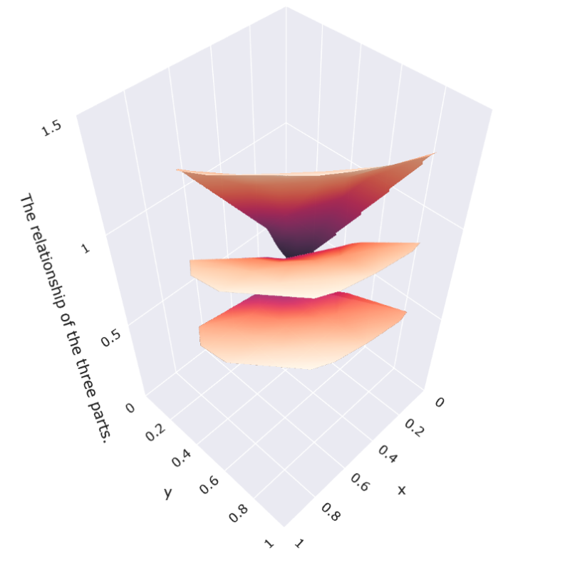
Figure 7: The relationship between the three parts.

Example IV.2.

Given a FoD $\Theta=\{{{e}_{1}},{{e}_{2}}\}$, let a CBBA $\mathbb{M}$ be defined in the FoD. There are also two variable parameters $x$ and $y$ in the defined CBBA. The CBBA is given as below

$$\mathbb{M}({{e}_{1}})=(1-x)-yi,$$

$$\mathbb{M}({{e}_{1}},{{e}_{2}})=x+yi,$$

satisfying $\sqrt{{{x}^{2}}+{{y}^{2}}}\in[0,1]$ and $\sqrt{{{(1-x)}^{2}}+{{(-y)}^{2}}}\in[0,1]$.

Then according to Definition III.1, the FCBBA can be obtained

$${{\mathbb{M}}_{F}}({{e}_{1}})=\mathbb{M}({{e}_{1}})+\frac{\mathbb{M}({{e}_{1}},{{e}_{2}})}{3}=\frac{3-2x}{3}-\frac{2y}{3}i,$$

$${{\mathbb{M}}_{F}}({{e}_{2}})=\frac{\mathbb{M}({{e}_{1}},{{e}_{2}})}{3}=\frac{x}{3}+\frac{y}{3}i,$$

$${{\mathbb{M}}_{F}}({{e}_{1}},{{e}_{2}})=\frac{\mathbb{M}({{e}_{1}},{{e}_{2}})}{3}=\frac{x}{3}+\frac{y}{3}i.$$

With the change of the unknown number $x$ and $y$, the relationship between overall FCB entropy and discord and non-specificity is shown in Figure 7 .

V Experiments

The generation of FCBBA includes the process of assigning multi-element focal elements to its subsets, reflecting the impact of the intersection of different events on the system uncertainty measurement. Therefore, FCB entropy can be used to reflect the uncertainty in CBBA caused by the intersection of different events. Next, several specific examples are used to illustrate.

Example V.1.

The purpose of the question is to find the target element. Suppose there are two different sources of evidence, that is, two CBBAs are defined on a same FoD $X=\{{{x}_{1}},{{x}_{2}},{{x}_{3}},{{x}_{4}}\}$, the results of the two CBBAs are given as below.

$${{\mathbb{M}}_{1}}:{{\mathbb{M}}_{1}}(\{{{x}_{1}},{{x}_{2}}\})=0.4+0.2i,{{\mathbb{M}}_{1}}(\{{{x}_{3}},{{x}_{4}}\})=0.6-0.2i,$$

$${{\mathbb{M}}_{2}}:{{\mathbb{M}}_{2}}(\{{{x}_{1}},{{x}_{3}}\})=0.4+0.2i,{{\mathbb{M}}_{1}}(\{{{x}_{2}},{{x}_{3}}\})=0.6-0.2i.$$

It can be seen from the two CBBAs that the four elements in the first evidence source may be the target elements, and the corresponding elements in the two complex mass functions given are different from each other. In the second evidence source, there are only three elements as possible target elements, and there is a same element ${{x}_{3}}$ in the two complex mass functions given. Therefore, it is intuitively judged that the conflict degree of ${{\mathbb{M}}_{1}}$ is higher than that of ${{\mathbb{M}}_{2}}$, that is, the uncertainty of ${{\mathbb{M}}_{2}}$ should be less than that of ${{\mathbb{M}}_{1}}$.

In order to compare the effect of FCB entropy and the previously proposed entropies on multi-element intersection, the previous entropies are extended to CBBA using Definition LABEL:def2.16. The calculation results of each entropy are shown in Table VIII.

TABLE VIII: Results of different entropies in Example V.1.

	Entropy
$\mathbb{M}$	Pal et al. [37]	Deng [35]	Zhou et al. [64]	Cui et al. [62]	FCB
$\mathbb{M}_{1}$	1.9787	2.5636	2.2029	2.5636	2.5636
$\mathbb{M}_{2}$	1.9787	2.5636	2.2029	2.0827	2.2529

From Table VIII, it is obvious that Pal et al.’s entropy, Deng entropy, Zhou et al. s’entropy did not take into account the change in the amount of information caused by the intersection of focal elements, so the entropy of the two evidence sources is the same, resulting in information loss. Only the uncertainty of FCB entropy measurement meets the requirement that ${{\mathbb{M}}_{1}}$ is greater than ${{\mathbb{M}}_{2}}$. Logically, ${{\mathbb{M}}_{1}}$ should contain more information because the uncertainty is greater than ${{\mathbb{M}}_{2}}$. Therefore, the newly proposed FCB entropy is more effective in reducing information loss.

Here, another example is given to verify its effectiveness in measuring uncertain information.

Example V.2.

In this example, there are three different CBBAs based on different FoDs, that is, the number of elements is different. The three CBBA values are as follows

$${{\mathbb{M}}_{1}}: {{\mathbb{M}}_{1}}(\{{{x}_{1}},{{x}_{2}}\})=0.2+0.1i,{{\mathbb{M}}_{1}}(\{{{x}_{3}},{{x}_{4}}\})=0.6+0.2i,$$

$${{\mathbb{M}}_{1}}(\{{{x}_{5}},{{x}_{6}}\})=0.2-0.3i,$$

$${{\mathbb{M}}_{2}}: {{\mathbb{M}}_{2}}(\{{{x}_{1}},{{x}_{2}}\})=0.2+0.1i,{{\mathbb{M}}_{2}}(\{{{x}_{2}},{{x}_{3}}\})=0.6+0.2i,$$

$${{\mathbb{M}}_{2}}(\{{{x}_{3}},{{x}_{6}}\})=0.2-0.3i,$$

$${{\mathbb{M}}_{3}}: {{\mathbb{M}}_{3}}(\{{{x}_{1}},{{x}_{2}}\})=0.2+0.1i,{{\mathbb{M}}_{3}}(\{{{x}_{2}},{{x}_{3}}\})=0.6+0.2i,$$

$${{\mathbb{M}}_{3}}(\{{{x}_{5}},{{x}_{6}}\})=0.2-0.3i.$$

Intuitively, the uncertainty of evidence source 1 should be the largest, and that of evidence source 2 should be the smallest. The calculation results of several different entropy of three different evidence sources are shown in Figure 8 and Table IX. From Figure 8 and Table IX, it can be seen that Pal et al.’s entropy, Deng entropy and Zhou et al. s’entropy cannot reflect the change in the amount of information caused by the intersection of focal elements. Cui et al. s’entropy and the proposed FCB entropy can reflect this feature, and the change trend of FCB entropy is more obvious than Cui et al. s’entropy, so FCB entropy is more effective and has a good description ability for uncertain information.

TABLE IX: Results of different entropy in Example V.2.

	Entropy
$\mathbb{M}$	Pal et al. [37]	Deng [35]	Zhou et al. [64]	Cui et al. [62]	FCB
$\mathbb{M}_{1}$	2.4598	3.0448	2.6841	3.0448	3.0448
$\mathbb{M}_{2}$	2.4598	3.0448	2.6841	3.0100	2.6263
$\mathbb{M}_{3}$	2.4598	3.0448	2.6841	3.0287	2.8508

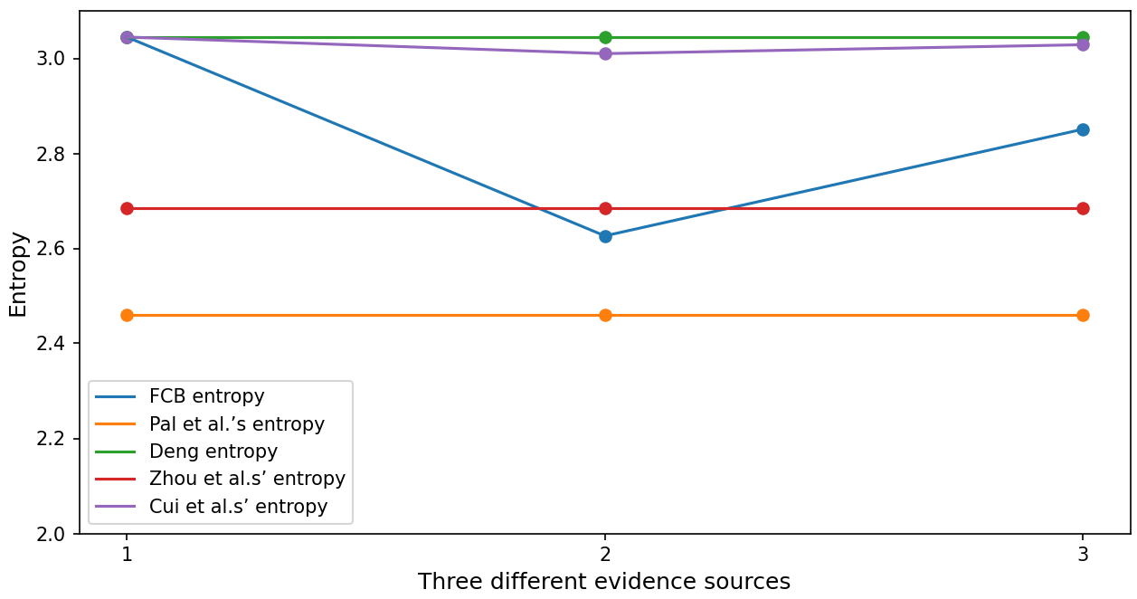
Figure 8: Line chart of calculation results of different entropy in Example V.2.

Example V.3.

Given a FoD $X=\{{{x}_{1}},{{x}_{2}},\cdots,{{x}_{10}}\}$ and a CBBA $\mathbb{M}$ defined on the FoD is given as follows

$$\mathbb{M}({{x}_{1}})=\alpha+0.3i,$$

$$\mathbb{M}({{X}_{i}})=1-\alpha-0.3i.$$

The complex mass assignment in $\mathbb{M}$ varies with the number of elements in ${{X}_{i}}$ ,which is shown in Table X. In addition, the complex mass assignment in $\mathbb{M}$ varies with $\alpha$. Next, set the value of $\alpha$ to 0, 0.1. In the case of taking two different values of a, the results of FCB entropy, Deng entropy [35], Zhou et al.’s entropy [64] changing with the change of $i$ are shown in Figures 9a, 9b.

TABLE X: Results of different entropy in Example V.2.

$i$	$X_{i}$
1	$x_{1}$
2	$x_{1}$, $x_{2}$
3	$x_{1}$, $x_{2}$, $x_{3}$
4	$x_{1}$, $x_{2}$, $x_{3}$, $x_{4}$
5	$x_{1}$, $x_{2}$, $x_{3}$, $x_{4}$, $x_{5}$
6	$x_{1}$, $x_{2}$, $x_{3}$, $x_{4}$, $x_{5}$, $x_{6}$
7	$x_{1}$, $x_{2}$, $x_{3}$, $x_{4}$, $x_{5}$, $x_{6}$, $x_{7}$
8	$x_{1}$, $x_{2}$, $x_{3}$, $x_{4}$, $x_{5}$, $x_{6}$, $x_{7}$, $x_{8}$
9	$x_{1}$, $x_{2}$, $x_{3}$, $x_{4}$, $x_{5}$, $x_{6}$, $x_{7}$, $x_{8}$, $x_{9}$
10	$x_{1}$, $x_{2}$, $x_{3}$, $x_{4}$, $x_{5}$, $x_{6}$, $x_{7}$, $x_{8}$, $x_{9}$, $x_{10}$

From the two figures, it can be seen that when $i=1$, all the mass is allocated to the single element focal element ${{x}_{1}}$. From the logical judgment, ${{x}_{1}}$ is certain, and the uncertainty should be 0. However, only the FCB entropy of the three entropy is 0, which is consistent with objective cognition. As $i$ increases, FCB entropy is basically consistent with Deng entropy. That is, FCB entropy has the performance of measuring uncertainty similar to Deng entropy. And with the increase of $\alpha$, the mass distribution of ${{x}_{1}}$ increases and the uncertainty decreases. The above three kinds of entropy can well reflect this phenomenon. To sum up, FCB entropy has advantages in measuring uncertainty.

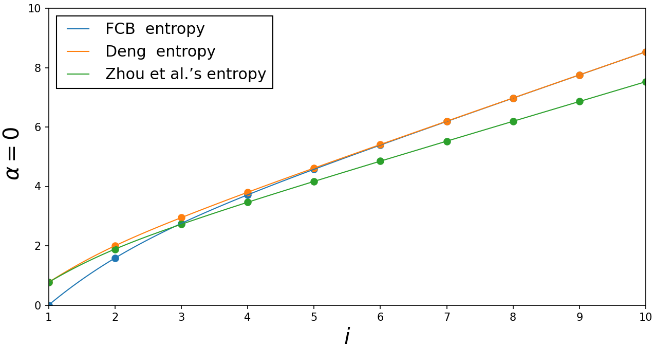
(a) When $\alpha=0$, the curves of three entropies changes with $i$.

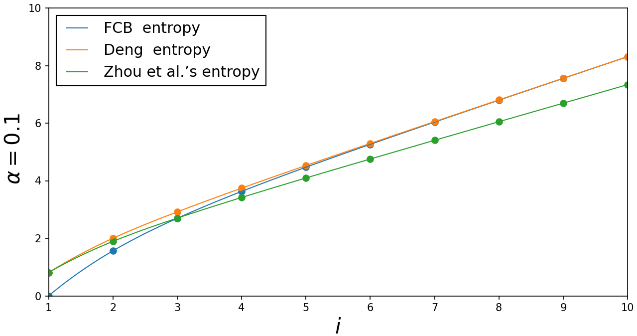
(b) When $\alpha=0.1$, the curves of three entropies changes with $i$.

Figure 9: Three entropies change with $i$ when $\alpha$ sets different values.

VI Conclusions

As a generalization of D-S evidence theory, complex evidence theory has played an important role in many fields. However, the measurement of uncertainty is still an open issue. Many studies have proposed different measurement methods, such as belief entropy, divergence, etc. As a new subject, fractal theory has attracted many scholars’ interest. In order to link CBBA with probability, a CPBT method is proposed to convert CBBA into probability. However, CPBT only gives the result of conversion without specific process. Therefore, the relationship between CBBA and probability cannot be comprehensively understood. Inspired by fractal theory, this paper proposes a fractal generation process of CPBT. Then, based on the generation process of CPBT, a new basic belief assignment called FCBBA is defined, and on this basis, FCB entropy is proposed to measure the uncertainty of CBBA. The discord and non-specificity are also defined. Then the properties of FCB entropy are analyzed, and several examples are used to verify its effectiveness. In the future, the application of FCB entropy in pattern recognition, evidence fusion and other fields will be analyzed and realized.

References

- [1] Chenhui Qiang, Yong Deng, and Kang Hao Cheong. Information fractal dimension of mass function. Fractals, 30:2250110, 2022.
- [2] Ruonan Zhu, Qing Liu, Chongru Huang, and Bingyi Kang. Z-ACM: An approximate calculation method of Z-numbers for large data sets based on kernel density estimation and its application in decision-making. Information Sciences, 610:440–471, 2022.
- [3] Ran Tao, Zeyi Liu, Rui Cai, and Kang Hao Cheong. A dynamic group MCDM model with intuitionistic fuzzy set: Perspective of alternative queuing method. Information Sciences, 555:85–103, 2021.
- [4] Yafei Song, Qiang Fu, Yi-Fei Wang, and Xiaodan Wang. Divergence-based cross entropy and uncertainty measures of Atanassov’s intuitionistic fuzzy sets with their application in decision making. Applied Soft Computing, 84:105703, 2019.
- [5] Hamido Fujita, Angelo Gaeta, Vincenzo Loia, and Francesco Orciuoli. Hypotheses analysis and assessment in counter-terrorism activities: a method based on OWA and fuzzy probabilistic rough sets. IEEE Transactions on Fuzzy Systems, 28:831–845, 2020.
- [6] Jin Ye, Jianming Zhan, Weiping Ding, and Hamido Fujita. A novel fuzzy rough set model with fuzzy neighborhood operators. Information Sciences, 544:266–297, 2021.
- [7] Yong Deng. Random permutation set. International Journal of Computers Communications & Control, 17(1):4542, 2022.
- [8] Yong Deng. Information volume of mass function. International Journal of Computers Communications & Control, 15(6), 2020.
- [9] Leihui Xiong, Xiaoyan Su, and Hong Qian. Conflicting evidence combination from the perspective of networks. Information Sciences, 580:408–418, 2021.
- [10] Leilei Chang, Limao Zhang, Chao Fu, and Yu-Wang Chen. Transparent digital twin for output control using belief rule base. IEEE Transactions on Cybernetics, page DOI: 10.1109/TCYB.2021.3063285, 2021.
- [11] Zhen Hua, Liguo Fei, and Huifeng Xue. Consensus reaching with dynamic expert credibility under Dempster-Shafer theory. Information Sciences, 610:847–867, 2022.
- [12] Yuelin Che, Yong Deng, and Yu-Hsi Yuan. Maximum-entropy-based decision-making trial and evaluation laboratory and its application in emergency management. Journal of Organizational and End User Computing (JOEUC), 34(7):1–16, 2022.
- [13] Fuyuan Xiao, Junhao Wen, and Witold Pedrycz. Generalized divergence-based decision making method with an application to pattern classification. IEEE Transactions on Knowledge and Data Engineering, page DOI: 10.1109/TKDE.2022.3177896, 2022.
- [14] Huchang Liao, Xiaofang Li, and Ming Tang. How to process local and global consensus? a large-scale group decision making model based on social network analysis with probabilistic linguistic information. Information Sciences, 579:368–387, 2021.
- [15] Harish Garg and Shyi-Ming Chen. Multiattribute group decision making based on neutrality aggregation operators of q-rung orthopair fuzzy sets. Information Sciences, 517:427–447, 2020.
- [16] Ya-Jing Zhou, Mi Zhou, Xin-Bao Liu, Ba-Yi Cheng, and Enrique Herrera-Viedma. Consensus reaching mechanism with parallel dynamic feedback strategy for large-scale group decision making under social network analysis. Computers & Industrial Engineering, 174:108818, 2022.
- [17] Mi Zhou, Ya-Qian Zheng, Yu-Wang Chen, Ba-Yi Cheng, Enrique Herrera-Viedma, and Jian Wu. A large-scale group consensus reaching approach considering self-confidence with two-tuple linguistic trust/distrust relationship and its application in life cycle sustainability assessment. Information Fusion, 94:181–199, 2023.
- [18] Xinyang Deng and Yebi Cui. An improved belief structure satisfaction to uncertain target values by considering the overlapping degree between events. Information Sciences, 580:398–407, 2021.
- [19] Zhunga Liu, Yu Liu, Jean Dezert, and Fabio Cuzzolin. Evidence combination based on credal belief redistribution for pattern classification. IEEE Transactions on Fuzzy Systems, 28(4):618–631, 2020.
- [20] Dingbin Li, Yong Deng, and Kang Hao Cheong. Multisource basic probability assignment fusion based on information quality. International Journal of Intelligent Systems, 36(4):1851–1875, 2021.
- [21] Fuyuan Xiao. GEJS: A generalized evidential divergence measure for multisource information fusion. IEEE Transactions on Systems, Man, and Cybernetics - Systems, page DOI: 10.1109/TSMC.2022.3211498, 2022.
- [22] Caosheng Zhu, Fuyuan Xiao, and Zehong Cao. A generalized Rényi divergence for multi-source information fusion with its application in EEG data analysis. Information Sciences, page DOI: 10.1016/j.ins.2022.05.012, 2022.
- [23] Qiuyan Shang, Hanwen Li, Yong Deng, and Kang Hao Cheong. Compound credibility for conflicting evidence combination: an autoencoder-K-Means approach. IEEE Transactions on Systems, Man, and Cybernetics: Systems, page 10.1109/TSMC.2021.3130187, 2021.
- [24] Fuyuan Xiao, Zehong Cao, and Chin-Teng Lin. A complex weighted discounting multisource information fusion with its application in pattern classification. IEEE Transactions on Knowledge and Data Engineering, page DOI: 10.1109/TKDE.2022.3206871, 2022.
- [25] Chao Fu, Qianshan Zhan, and Weiyong Liu. Evidential reasoning based ensemble classifier for uncertain imbalanced data. Information Sciences, 578:378–400, 2021.
- [26] Xiaobin Xu, Deqing Zhang, Yu Bai, Leilei Chang, and Jianning Li. Evidence reasoning rule-based classifier with uncertainty quantification. Information Sciences, 516:192–204, 2020.
- [27] Jie Wang, Zhijie Zhou, Changhua Hu, Shuaiwen Tang, Wei He, and Tengyu Long. A fusion approach based on evidential reasoning rule considering the reliability of digital quantities. Information Sciences, 612:107–131, 2022.
- [28] Debiao Meng, Hongtao Wang, Shiyuan Yang, Zhiyuan Lv, Zhengguo Hu, and Zihao Wang. Fault analysis of wind power rolling bearing based on EMD feature extraction. CMES-Computer Modeling in Engineering & Sciences, 130(1):543–558, 2022.
- [29] Xingyuan Chen and Yong Deng. An evidential software risk evaluation model. Mathematics, 10(13):10.3390/math10132325, 2022.
- [30] Zhen Wang, Zhaoqing Li, Rong Wang, Feiping Nie, and Xuelong Li. Large graph clustering with simultaneous spectral embedding and discretization. IEEE Transactions on Pattern Analysis and Machine Intelligence, 43(12):4426–4440, 2021.
- [31] Bo Wei, Feng Xiao, Fang Fang, and Yang Shi. Velocity-free event-triggered control for multiple euler–lagrange systems with communication time delays. IEEE Transactions on Automatic Control, 66(11):5599–5605, 2021.
- [32] Yan-Feng Li, Hong-Zhong Huang, Jinhua Mi, Weiwen Peng, and Xiaomeng Han. Reliability analysis of multi-state systems with common cause failures based on Bayesian network and fuzzy probability. Annals of Operations Research, 311:195–209, 2022.
- [33] Lei Ni, Yu-wang Chen, and Oscar de Brujin. Towards understanding socially influenced vaccination decision making: An integrated model of multiple criteria belief modelling and social network analysis. European Journal of Operational Research, 293(1):276–289, 2021.
- [34] Luyuan Chen, Yong Deng, and Kang Hao Cheong. Probability transformation of mass function: A weighted network method based on the ordered visibility graph. Engineering Applications of Artificial Intelligence, 105:104438, 2021.
- [35] Yong Deng. Uncertainty measure in evidence theory. Science China Information Sciences, 63(11):210201, 2020.
- [36] Didier Dubois and Henri Prade. Properties of measures of information in evidence and possibility theories. Fuzzy Sets and Systems, 24(2):161–182, 1987.
- [37] Nikhil R Pal, James C Bezdek, and Rohan Hemasinha. Uncertainty measures for evidential reasoning i: A review. International Journal of Approximate Reasoning, 7(3-4):165–183, 1992.
- [38] A-L Jousselme, Chunsheng Liu, Dominic Grenier, and Éloi Bossé. Measuring ambiguity in the evidence theory. IEEE Transactions on Systems, Man, and Cybernetics-Part A: Systems and Humans, 36(5):890–903, 2006.
- [39] Radim Jiroušek and Prakash P Shenoy. A new definition of entropy of belief functions in the dempster–shafer theory. International Journal of Approximate Reasoning, 92:49–65, 2018.
- [40] Qian Pan, Deyun Zhou, Yongchuan Tang, Xiaoyang Li, and Jichuan Huang. A novel belief entropy for measuring uncertainty in dempster-shafer evidence theory framework based on plausibility transformation and weighted hartley entropy. Entropy, 21(2):163, 2019.
- [41] Yong Deng. Deng entropy. Chaos, Solitons & Fractals, 91:549–553, 2016.
- [42] Zehong Cao, Chin-Teng Lin, Kuan-Lin Lai, Li-Wei Ko, Jung-Tai King, Kwong-Kum Liao, Jong-Ling Fuh, and Shuu-Jiun Wang. Extraction of SSVEPs-based inherent fuzzy entropy using a wearable headband EEG in migraine patients. IEEE Transactions on Fuzzy Systems, 28(1):14–27, 2019.
- [43] Peide Liu, Mengjiao Shen, Fei Teng, Baoying Zhu, Lili Rong, and Yushui Geng. Double hierarchy hesitant fuzzy linguistic entropy-based TODIM approach using evidential theory. Information Sciences, 547:223–243, 2021.
- [44] Xiaodan Wang and Yafei Song. Uncertainty measure in evidence theory with its applications. Applied Intelligence, 48(7):1672–1688, 2018.
- [45] Yi Yang and Deqiang Han. A new distance-based total uncertainty measure in the theory of belief functions. Knowledge-Based Systems, 94:114–123, 2016.
- [46] Deqiang Han, Jean Dezert, and Yi Yang. Belief interval-based distance measures in the theory of belief functions. IEEE Transactions on Systems, Man, and Cybernetics: Systems, 48(6):833–850, 2018.
- [47] Yager, Ronald R. Entropy and specificity in a mathematical theory of evidence. In Classic works of the Dempster-Shafer theory of belief functions, pages 291–310. Springer, 2008.
- [48] Ronald R Yager, Naif Alajlan, and Yakoub Bazi. Uncertain database retrieval with measure-based belief function attribute values. Information Sciences, 501:761–770, 2019.
- [49] Hamido Fujita and Yu-Chien Ko. A heuristic representation learning based on evidential memberships: Case study of UCI-SPECTF. International Journal of Approximate Reasoning, 120, 2020.
- [50] Yager, Ronald R. On the fusion of imprecise uncertainty measures using belief structures. Information Sciences, 181(15):3199–3209, 2011.
- [51] Xiao, Fuyuan. Generalization of dempster–shafer theory: A complex mass function. Applied Intelligence, 50(10):3266–3275, 2020.
- [52] Xiao, Fuyuan. Generalized belief function in complex evidence theory. Journal of Intelligent & Fuzzy Systems, 38(4):3665–3673, 2020.
- [53] Wentao Fan and Fuyuan Xiao. A complex Jensen-Shannon divergence in complex evidence theory with its application in multi-source information fusion. Engineering Applications of Artificial Intelligence, page DOI: 10.1016/j.engappai.2022.105362, 2022.
- [54] Shengjia Zhang and Fuyuan Xiao. A TFN-based uncertainty modeling method in complex evidence theory for decision making. Information Sciences, page DOI: 10.1016/j.ins.2022.11.014, 2022.
- [55] Chengxi Yang and Fuyuan Xiao. An exponential negation of complex basic belief assignment in complex evidence theory. Information Sciences, 622:1228–1251, 2023.
- [56] Fuyuan Xiao and Witold Pedrycz. Negation of the quantum mass function for multisource quantum information fusion with its application to pattern classification. IEEE Transactions on Pattern Analysis and Machine Intelligence, page DOI: 10.1109/TPAMI.2022.3167045, 2022.
- [57] Fuyuan Xiao. Generalized quantum evidence theory. Applied Intelligence, pages DOI: 10.1007/s10489–022–04181–0, 2022.
- [58] Philippe Smets. Decision making in the tbm: the necessity of the pignistic transformation. International journal of approximate reasoning, 38(2):133–147, 2005.
- [59] Barry R Cobb and Prakash P Shenoy. On the plausibility transformation method for translating belief function models to probability models. International journal of approximate reasoning, 41(3):314–330, 2006.
- [60] Qianli Zhou and Yong Deng. Fractal-based belief entropy. Information Sciences, 587:265–282, 2022.
- [61] Fuyuan Xiao. Complex pignistic transformation-based evidential distance for multisource information fusion of medical diagnosis in the iot. Sensors, 21(3):840, 2021.
- [62] Huizi Cui, Qing Liu, Jianfeng Zhang, and Bingyi Kang. An improved deng entropy and its application in pattern recognition. IEEE Access, 7:18284–18292, 2019.
- [63] Masahiko Higashi and George J Klir. Measures of uncertainty and information based on possibility distributions. International journal of general systems, 9(1):43–58, 1982.
- [64] Mi Zhou, Yu-Wang Chen, Xin-Bao Liu, Ba-Yi Cheng, and Jian-Bo Yang. Weight assignment method for multiple attribute decision making with dissimilarity and conflict of belief distributions. Computers & Industrial Engineering, 147:106648, 2020.