The Quantum Kalman Decomposition: A Gramian Matrix Approach

Abstract

The Kalman canonical form for quantum linear systems was derived in [66]. The purpose of this paper is to present an alternative derivation by means of a Gramian matrix approach. Controllability and observability Gramian matrices are defined for linear quantum systems, which are used to characterize various subspaces. Based on these characterizations, real orthogonal and block symplectic coordinate transformation matrices are constructed to transform a given quantum linear system to the Kalman canonical form. An example is used to illustrate the main results.

keywords. quantum linear control systems, quantum Kalman canonical form, Gramian matrix

1 Introduction

In recent decades, significant advancements have been made in both theoretical understanding and experimental applications of quantum control. Quantum control plays a pivotal role in various quantum information technologies, such as quantum communication, quantum computation, quantum cryptography, quantum ultra-precision metrology, and nano-electronics. Similar to classical control systems theory, linear quantum systems hold great importance in the field of quantum control. Quantum linear systems are mathematical models that describe the behavior of quantum harmonic oscillators. In this context, “linear” refers to the linearity of the Heisenberg equations of motion for quadrature operators in the quantum systems. This linearity often leads to simplifications that facilitate analysis and control of these systems. Consequently, quantum linear systems can be effectively studied using powerful mathematical techniques derived from classical linear systems theory. A wide range of quantum-mechanical systems can be suitably modeled as quantum linear systems. For instance, quantum optical systems [58, 14, 57, 36, 59, 68, 46, 7, 43, 47, 4], circuit quantum electro-dynamical (circuit QED) systems [39, 6, 31, 5], cavity QED systems [11, 51, 1], quantum opto-mechanical systems [54, 38, 22, 12, 37, 63, 62, 2, 44, 30, 34, 48, 10], atomic ensembles [53, 42, 63, 3, 30], and quantum memories [61, 24, 25, 64, 40].

Due to their quantum-mechanical nature, quantum linear systems exhibit several unique control-theoretical properties that do not generally exist in the classical regime. Firstly, stabilizability is equivalent to detectability ([59, Section 6.6]) and controllability is equivalent to observability ([19, Proposition 1]). Secondly, Hurwitz stability implies both controllability and observability ([70, Theorem 3.1]). Thirdly, if the system is passive, then Hurwitz stability, controllability, and observability are all equivalent ([21],[19, Lemma 2]). Lastly, the controllable and unobservable subsystem coexists with the uncontrollable and observable subsystem [66].

The Kalman canonical form, initially proposed for classical linear systems by Kalman in 1963 [28, 29], has recently been extended to quantum linear systems [66, 70], where real orthogonal and block symplectic coordinate transformation matrices are constructed that transform a quantum linear system into a new one composed of four possible subsystems: the controllable and observable ($co$) subsystem, the controllable and unobservable ($c\bar{o}$) subsystem, the uncontrollable and observable ($\bar{c}o$) subsystem, and the uncontrollable and unobservable ($\bar{c}\bar{o}$) subsystem. The combination of the $c\bar{o}$ subsystem and the $\bar{c}o$ subsystem is referred to as the “$h$” subsystem. As shown in Fig. 1, the quantum Kalman canonical form retains the same structure as the classical version but possesses unique properties due to the distinct characteristics of quantum linear systems. Firstly, the controllable and unobservable ($c\bar{o}$) subsystem coexists with the uncontrollable and observable ($\bar{c}o$) subsystem. Secondly, in the case of a passive system, both the $c\bar{o}$ and $\bar{c}o$ subsystems vanish. Thirdly, the $A$-matrix of the “$h$” subsystem and the $A$-matrix of the $\bar{c}\bar{o}$ subsystem are Hamiltonian matrices. In addition to these control-theoretical implications, the quantum Kalman canonical form also provides insights into important physical concepts. For example, the $\bar{c}\bar{o}$ subsystem represents the decoherence-free subsystems (DFSs), and quantum non-demolition (QND) variables reside within the $\bar{c}o$ subsystem, indicating that their temporal evolution remains unaffected by the input probe or any complementary variables, while still being observable from the output probe. Finally, the determination of quantum back-action evading (BAE) measurement relies solely on the $co$ subsystem.

The quantum Kalman canonical form is very effective in demonstrating properties of quantum systems. For example, an opto-mechanical system was first theoretically studied in [60], and later on its experimental implementation was reported in [44]. This experimental setup successfully demonstrated quantum BAE measurements. In our 2018 paper [66, Example 5.2], this particular opto-mechanical system was thoroughly examined. By means of the quantum Kalman decomposition, Equation (83) of [66] was obtained which revealed the existence of quantum BAE measurements within this system. Additionally, Equation (83) of [66] also predicted the presence of quantum QND variables, denoted as $\boldsymbol{p}_{h}$ in that equation. Interestingly, a recent experiment conducted in 2021 [34] demonstrated QND variables precisely corresponding to $\boldsymbol{p}_{h}$ in Equation (83) of [66]. This finding suggests that Equation (83) in [66] provides an explanation for both the 2016 quantum BAE experiment [44] and the 2021 QND experiment [34], thus validating the effectiveness of the quantum Kalman canonical form in the study of quantum linear systems theory and experimental quantum physics.

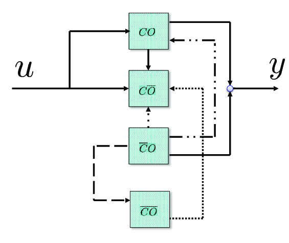
Figure 1: The Kalman canonical form of a quantum linear system; see [66, Fig. 2].

In [66], we start from the annihilation-creation operator representation of quantum linear systems and construct a unitary and block Bogoliubov transformation matrix, then we convert it to a real orthogonal and block symplectic transformation matrix in the quadrature representation. In this paper, we work in the quadrature representation and directly construct real orthogonal and block symplectic transformation matrices. In particular, we use controllability and observability Gramian matrices as the main tools in the construction.

The subsequent sections of this paper are organized as follows. In Section 2, we briefly review quantum linear systems. The observability and controllability Gramian matrices are presented in Section 3, and used to characterize various subspaces. The construction of the Kalman decomposition for quantum linear systems is given in Section 4. In Section 5 , a computational procedure is given for the construction of coordinate transformation matrices. In Section 6, an example in the literature is used for demonstration. Section 7 concludes this paper.

Notation.

• $\imath=\sqrt{-1}$ is the imaginary unit. $I_{k}$ is the identity matrix and $0_{k}$ the zero matrix in $\mathbb{C}^{k\times k}$. $\delta_{ij}$ denotes the Kronecker delta; i.e., $I_{k}=[\delta_{ij}]$. $\delta(t)$ is the Dirac delta function.

• $\Re(X)$ denotes the real part of $X$ which can be a scalar, vector or matrix, and $\Im(X)$ denotes its imaginary part.

• $x^{\ast}$ denotes the complex conjugate of a complex number $x$ or the adjoint of an operator $x$. Clearly. $(xy)^{\ast}=y^{\ast}x^{\ast}$.

• For a matrix $X=[x_{ij}]$ with number or operator entries, $X^{\top}=[x_{ji}]$ is the matrix transpose. Denote $X^{\#}=[x_{ij}^{\ast}]$, and $X^{\dagger}=(X^{\#})^{\top}$. For a vector $x$, we define $\breve{x}\triangleq\bigl{[}\begin{smallmatrix}x\\ x^{\#}\end{smallmatrix}\bigr{]}$.

• Given two operators $\mathbf{x}$ and $\mathbf{y}$, their commutator is defined to be $[\mathbf{x},\mathbf{y}]\triangleq\mathbf{x}\mathbf{y}-\mathbf{y}\mathbf{x}$. Given two column vectors of operators $\mathbf{X}$ and $\mathbf{Y}$, their commutator is defined as

  $$[\mathbf{X},\mathbf{Y}^{\top}]\triangleq([\mathbf{X}_{j},\mathbf{Y}_{k}])=\mathbf{X}\mathbf{Y}^{\top}-(\mathbf{Y}\mathbf{X}^{\top})^{\top}.$$ (1.1)

• Let $J_{k}\triangleq\mathrm{diag}(I_{k},-I_{k})$. For a matrix $X\in\mathbb{C}^{2k\times 2r}$, define its $\flat$-adjoint to be $X^{\flat}\triangleq J_{r}X^{\dagger}J_{k}$. The $\flat$-adjoint operation enjoys the following properties:

  $$(\alpha A+\beta B)^{\flat}=\alpha^{*}A^{\flat}+\beta^{*}B^{\flat},\ \ (AB)^{\flat}=B^{\flat}A^{\flat},\ \ (A^{\flat})^{\flat}=A,$$ (1.2)

  where $\alpha,\beta\in\mathbb{C}$.

• Given two matrices $U$, $V\in\mathbb{C}^{k\times r}$, define their doubled-up matrix [18] as $\Delta(U,V)\triangleq\bigl{[}\begin{smallmatrix}U&V\\ V^{\#}&U^{\#}\end{smallmatrix}\bigr{]}$. The set of doubled-up matrices is closed under addition, multiplication and $\flat$ adjoint operations.

• A matrix $T\in\mathbb{C}^{2k\times 2k}$ is called Bogoliubov if it is doubled-up and satisfies $TT^{\flat}=T^{\flat}T=I_{2k}$. The set of Bogoliubov matrices forms a complex non-compact Lie group known as the Bogoliubov group.

• Let $\mathbb{J}_{k}\triangleq\bigl{[}\begin{smallmatrix}0_{k}&I_{k}\\ -I_{k}&0_{k}\end{smallmatrix}\bigr{]}$. For a matrix $X\in\mathbb{C}^{2k\times 2r}$, define its $\sharp$-adjoint $X^{\sharp}$ as $X^{\sharp}\triangleq-\mathbb{J}_{r}X^{\dagger}\mathbb{J}_{k}$. The $\sharp$-adjoint satisfies properties similar to the usual adjoint, namely

  $$(\alpha A+\beta B)^{\sharp}=\alpha^{*}A^{\sharp}+\beta^{*}B^{\sharp},\ \ (AB)^{\sharp}=B^{\sharp}A^{\sharp},\ \ (A^{\sharp})^{\sharp}=A,$$ (1.3)

  where $\alpha,\beta\in\mathbb{C}$.

• A matrix $\mathbb{S}\in\mathbb{C}^{2k\times 2k}$ is called symplectic, if $\mathbb{S}\mathbb{S}^{\sharp}=\mathbb{S}^{\sharp}\mathbb{S}=I_{2k}$. Symplectic matrices forms a complex non-compact group known as the symplectic group. The subgroup of real symplectic matrices is one-to-one homomorphic to the Bogoliubov group.

• A square matrix $M$ is called a Hamiltonian matrix if $(\mathbb{J}M)^{\top}=\mathbb{J}M$. $M^{2}$ is skew-Hamiltonian as $\mathbb{J}M^{2}=-(\mathbb{J}M^{2})^{\top}$; See [15, Section 7.8].

• The reduced Planck constant $\hbar$ is set to 1 in this paper.

2 Linear quantum systems

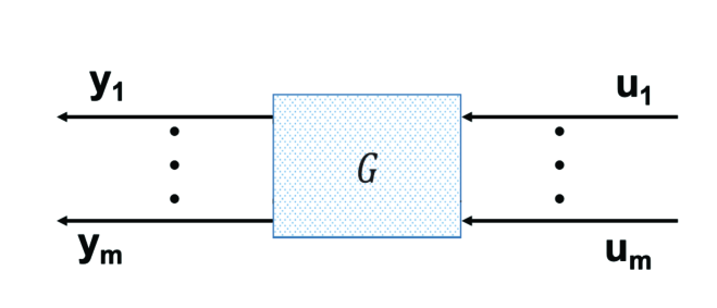
Figure 2: A quantum linear system. Here $G$ consists of $n$ quantum harmonic oscillators.

The quantum linear system, as shown in Figure 2, can be used to model a collection of $n$ quantum harmonic oscillators driven by $m$ input fields. The quadratures of the $j$-th quantum harmonic oscillator are denoted by $\mathbf{q}_{j}$ and $\mathbf{p}_{j}$ which satisfy the canonical commutation relations $[\mathbf{q}_{j}(t),\ \mathbf{p}_{j}(t)]=\imath$. The $k$-th input field is denoted by $\mathbf{u}_{k}$ whose quadratures $\mathbf{q}_{{\rm in},k}$ and $\mathbf{p}_{{\rm in},k}$ satisfy the singular commutation relation $[\mathbf{q}_{{\rm in},k}(t),\ \mathbf{p}_{{\rm in},k}(r)]=\imath\delta(t-r)$. Similarly, the $k$-th out field is denoted by $\mathbf{y}_{k}$ whose quadratures $\mathbf{q}_{{\rm out},k}$ and $\mathbf{p}_{{\rm out},k}$ satisfy the singular commutation relation $[\mathbf{q}_{{\rm out},k}(t),\ \mathbf{p}_{{\rm out},k}(r)]=\imath\delta(t-r)$. For notational convenience, we denote

$$\mathbf{q}(t)=\left[\begin{array}[]{c}\mathbf{q}_{1}(t)\\ \cdots\\ \mathbf{q}_{n}(t)\end{array}\right],\ \mathbf{p}(t)=\left[\begin{array}[]{c}\mathbf{p}_{1}(t)\\ \cdots\\ \mathbf{p}_{n}(t)\end{array}\right],\ \mathbf{q}_{\rm in}(t)=\left[\begin{array}[]{c}\mathbf{q}_{{\rm in},1}(t)\\ \cdots\\ \mathbf{q}_{{\rm in},m}(t)\end{array}\right],$$

$$\mathbf{p}_{\rm in}(t)=\left[\begin{array}[]{c}\mathbf{p}_{{\rm in},1}(t)\\ \cdots\\ \mathbf{p}_{{\rm in},m}(t)\end{array}\right],\ \mathbf{q}_{\rm out}(t)=\left[\begin{array}[]{c}\mathbf{q}_{{\rm out},1}(t)\\ \cdots\\ \mathbf{q}_{{\rm out},m}(t)\end{array}\right],\ \mathbf{p}_{\rm out}(t)=\left[\begin{array}[]{c}\mathbf{p}_{{\rm out},1}(t)\\ \cdots\\ \mathbf{p}_{{\rm out},m}(t)\end{array}\right].$$

Denote the system variables, inputs and outputs by

$$\left[\begin{array}[]{c}\mathbf{q}(t)\\ \mathbf{p}(t)\end{array}\right]\equiv\mathbf{x}(t),\ \ \left[\begin{array}[]{c}\mathbf{q}_{\mathrm{in}}(t)\\ \mathbf{p}_{\mathrm{in}}(t)\end{array}\right]\equiv\mathbf{u}(t),\ \ \left[\begin{array}[]{c}\mathbf{q}_{\mathrm{out}}(t)\\ \mathbf{p}_{\mathrm{out}}(t)\end{array}\right]\equiv\mathbf{y}(t),$$ (2.1)

respectively, which satisfy

$$[\mathbf{x}(t),\ \mathbf{x}(t)^{\top}]=\imath\mathbb{J}_{n},\ [\mathbf{u}(t),\ \mathbf{u}(r)^{\top}]=[\mathbf{y}(t),\ \mathbf{y}(r)^{\top}]=\imath\delta(t-r)\mathbb{J}_{m}.$$ (2.2)

It is often convenient to describe a quantum system’s dynamics in the $(S,\mathbf{L},\mathbf{H})$ formalism [16, 17], as it offers a powerful modelling framework for analyzing and designing networked quantum systems; see e.g., [36, 67, 68, 22, 23, 56, 33, 30, 35, 65, 50] and references therein. For the quantum linear system in Figure 2, $S\in\mathbb{C}^{m\times m}$ is a unitary matrix which can be used to model static devices such as phase shifters and beamsplitters. The operator $\mathbf{L}$ represents the interface between the system $G$ and its inputs, and the operator $\mathbf{H}$ describes the Hamiltonian of the system $G$. Mathematically, the coupling operator $\mathbf{L}$ and the Hamiltonian $\mathbf{H}$ are given by

$$\mathbf{L}= \;\Lambda\mathbf{x},$$ (2.3)

$$\mathbf{H}= \;\frac{1}{2}\mathbf{x}^{\top}\mathbb{H}\mathbf{x},$$

where $\Lambda\in\mathbb{C}^{m\times 2n}$, and $\mathbb{H}\in\mathbb{R}^{2n\times 2n}$ is symmetric.

The quantum stochastic differential equations (QSDEs) that describe the dynamics of the linear quantum system in Figure 2 in the real quadrature operator representation are the following:

$$\dot{\mathbf{x}}(t)= \;\mathbb{A}\mathbf{x}(t)+\mathbb{B}\mathbf{u}(t),$$ (2.4)

$$\mathbf{y}(t)= \;\mathbb{C}\mathbf{x}(t)+\mathbb{D}\mathbf{u}(t),$$

where the real static system matrices are

$$\mathbb{D}= \;\left[\begin{array}[]{cc}\Re(S)&-\Im(S)\\ \Im(S)&\Re(S)\end{array}\right],$$ (2.5)

$$\mathbb{C}= \;\sqrt{2}\left[\begin{array}[]{c}\Re(\Lambda)\\ \Im(\Lambda)\end{array}\right],$$

$$\mathbb{B}= \;-\mathbb{C}^{\sharp}\mathbb{D},$$

$$\mathbb{A}= \;\mathbb{J}_{n}\mathbb{H}-\frac{1}{2}\mathbb{C}^{\sharp}\mathbb{C}.$$

As the matrix $S$ is unitary, $\mathbb{D}\mathbb{D}^{\sharp}=I_{2m}$. In the real quadrature operator representation (2.4) of linear quantum systems, the physical realizability conditions ([26, 41, 18, 52, 68, 69]) take the form

$$\mathbb{A}+\mathbb{A}^{\sharp}+\mathbb{B}\mathbb{B}^{\sharp}=0,~{}\mathbb{B}=-\mathbb{C}^{\sharp}\mathbb{D}^{\sharp}.$$ (2.6)

As the scattering matrix $S$ does not affect the coordinate transformation to be performed, in the rest of this paper we assume $S=I_{m}$. Consequently, $\mathbb{D}=I_{2m}$ and $\mathbb{B}=-\mathbb{C}^{\sharp}$. This can also be understood by regarding $\mathbb{D}\mathbf{u}$ as the new input to the system. More discussions on quantum linear systems can be found in [26, 42, 67, 59, 63, 43, 66, 65] and references therein.

Note that while we use the same notation $\mathbb{C}$ for the set of complex numbers and the system $C$-matrix in (2.4), the distinction will be self-evident from the context.

3 Observability and controllability Gramian matrices

In this section, we define observability and controllability Gramian matrices for the quantum linear system (2.4), and then use them to characterize various subspaces of $\mathbb{R}^{2n}$.

For the quantum linear system (2.4), define the observability and controllability matrices to be

$$\mathbb{O}_{G}\triangleq\left[\begin{array}[]{c}\mathbb{C}\\ \mathbb{C}\mathbb{A}\\ \mathbb{C}\mathbb{A}^{2}\\ \vdots\\ \mathbb{C}\mathbb{A}^{2n-1}\end{array}\right],\ \ \ \mathbb{C}_{G}\triangleq\left[\begin{array}[]{ccccc}\mathbb{B}&\mathbb{A}\mathbb{B}&\mathbb{A}^{2}\mathbb{B}&\cdots&\mathbb{A}^{2n-1}\mathbb{B}\end{array}\right],$$ (3.1)

respectively. We also define two more matrices

$$\mathbb{O}_{s}\triangleq\left[\begin{array}[]{c}\mathbb{C}\\ \mathbb{C}\mathbb{J}_{n}\mathbb{H}\\ \mathbb{C}(\mathbb{J}_{n}\mathbb{H})^{2}\\ \vdots\\ \mathbb{C}(\mathbb{J}_{n}\mathbb{H})^{2n-1}\end{array}\right],\ \ \ \mathbb{C}_{s}\triangleq\left[\begin{array}[]{ccccc}\mathbb{B}&(\mathbb{J}_{n}\mathbb{H})\mathbb{B}&(\mathbb{J}_{n}\mathbb{H})^{2}\mathbb{B}&\cdots&(\mathbb{J}_{n}\mathbb{H})^{2n-1}\mathbb{B}\end{array}\right].$$ (3.2)

The matrices $\mathbb{O}_{s}$ and $\mathbb{C}_{s}$ are related by

$$\left[\begin{array}[]{ccccc}\mathbb{J}_{m}&&&&\\ &-\mathbb{J}_{m}&&&\\ &&\ddots&&\\ &&&\mathbb{J}_{m}&\\ &&&&-\mathbb{J}_{m}\end{array}\right]\mathbb{C}_{s}^{\top}\mathbb{J}_{n}=\mathbb{O}_{s}.$$ (3.3)

Consequently,

$${\rm Ker}(\mathbb{O}_{s})= \;{\rm Ker}(\mathbb{C}_{s}^{\top}\mathbb{J}_{n}),$$ (3.4)

$${\rm Ker}(\mathbb{O}_{s}\mathbb{J}_{n})= \;{\rm Ker}(\mathbb{C}_{s}^{\top})={\rm Im}(\mathbb{C}_{s})^{\perp}.$$

It can easily checked that

$${\rm Im}(\mathbb{C}_{G})={\rm Im}(\mathbb{C}_{s}),\ {\rm Ker}(\mathbb{O}_{G})={\rm Ker}(\mathbb{O}_{s}).$$ (3.5)

Hence, we use $\mathbb{O}_{s}$ and $\mathbb{C}_{s}$, instead of $\mathbb{O}_{G}$ and $\mathbb{C}_{G}$, in the following discussions as they appear simpler.

Remark 3.1

Notice that the matrix $\mathbb{O}_{s}$ defined in Eq. (3.2) is the real-domain counterpart of the matrix $\mathbf{O}_{s}$ defined in [19, Eq. (7)] in the complex domain.

Similar to the classical case, see e.g., [27] and [49, Chapter 9], define the observability Gramian matrix $W_{o}(t,s)$ and controllability Gramian matrix $W_{c}(t,s)$ to be

$$W_{o}(t,s)\triangleq\;\int_{t}^{s}e^{(\mathbb{J}_{n}\mathbb{H})^{\top}(\tau-t)}\mathbb{C}^{\top}\mathbb{C}e^{(\mathbb{J}_{n}\mathbb{H})(\tau-t)}d\tau,\ \ \forall-\infty<t<s<\infty,$$ (3.6a)

$$W_{c}(t,s)\triangleq\;\int_{t}^{s}e^{(\mathbb{J}_{n}\mathbb{H})(t-\tau)}\mathbb{B}\mathbb{B}^{\top}e^{(\mathbb{J}_{n}\mathbb{H})^{\top}(t-\tau)}d\tau,\ \ \forall-\infty<t<s<\infty,$$ (3.6b)

respectively. Clearly, both $W_{o}(t,s)$ and $W_{c}(t,s)$ are real and positive semi-definite matrices.

The following result reveals a nice relation between the observability and controllability Gramians which is unique to quantum linear systems,

Lemma 3.1

The observability Gramian $W_{o}(t,s)$ and controllability Gramian $W_{c}(t,s)$ are related by

$$W_{o}(t,s)=W_{c}(t,s)^{\sharp}.$$ (3.7)

Proof. Noticing that $\mathbb{J}_{n}^{\top}=-\mathbb{J}_{n}$ and $\mathbb{J}_{n}^{\top}e^{\mathbb{J}_{n}\mathbb{H}}\mathbb{J}_{n}=e^{\mathbb{H}\mathbb{J}_{n}}$, we have

$$W_{c}(t,s)^{\sharp} = \mathbb{J}_{n}^{\top}W_{c}(t,s)\mathbb{J}_{n}$$ (3.8)

$$= \int_{t}^{s}\mathbb{J}_{n}^{\top}e^{(\mathbb{J}_{n}\mathbb{H})(t-\tau)}\mathbb{B}\mathbb{B}^{\top}e^{(\mathbb{J}_{n}\mathbb{H})^{\top}(t-\tau)}\mathbb{J}_{n}d\tau$$

$$= \int_{t}^{s}\left(\mathbb{J}_{n}^{\top}e^{(\mathbb{J}_{n}\mathbb{H})(t-\tau)}\mathbb{J}_{n}\right)\left(\mathbb{J}_{n}^{\top}\mathbb{B}\mathbb{J}_{m}\right)\left(\mathbb{J}_{n}^{\top}\mathbb{B}\mathbb{J}_{m}\right)^{\top}\left(\mathbb{J}_{n}^{\top}e^{(\mathbb{J}_{n}\mathbb{H})(t-\tau)}\mathbb{J}_{n}\right)^{\top}d\tau$$

$$= \int_{t}^{s}\left(e^{(\mathbb{H}\mathbb{J}_{n})(t-\tau)}\right)\left(-\mathbb{C}^{\top}\right)\left(-\mathbb{C}\right)\left(e^{(\mathbb{H}\mathbb{J}_{n})(t-\tau)}\right)^{\top}$$

$$= \int_{t}^{s}e^{(\mathbb{J}_{n}\mathbb{H})^{\top}(\tau-t)}\mathbb{C}^{\top}\mathbb{C}e^{(\mathbb{J}_{n}\mathbb{H})(\tau-t)}d\tau$$

$$= W_{o}(t,s).$$

This completes the proof. $\Box$

In the following, We characterize various subspaces of $\mathbb{R}^{2n}$ in terms of the observability Gramian matrix $W_{o}(t,s)$ and controllability Gramian matrix $W_{c}(t,s)$.

We start from the following result.

Lemma 3.2

We have

$${\rm Ker}(\mathbb{O}_{s})={\rm Ker}(W_{o}(t,s)),\ \ \forall-\infty<t<s<\infty,$$ (3.9)

and

$${\rm Im}(\mathbb{O}_{s}^{\top})={\rm Im}(W_{o}(t,s)),\ \ \forall-\infty<t<s<\infty.$$ (3.10)

Proof. For each $x\in{\rm Ker}(\mathbb{O}_{s})$, by Eq. (3.2) we have $\mathbb{C}(\mathbb{J}_{n}\mathbb{H})^{k}x=0$ for all $k=0,1,\ldots,2n-1$. Hence, according to the Cayley-Hamilton theorem, $\mathbb{C}e^{(\mathbb{J}_{n}\mathbb{H})t}x=0$ for all $t\in\mathbb{R}$, which means that $x\in{\rm Ker}(W_{o}(t,s))$ for all $-\infty<t<s<\infty$. Hence, ${\rm Ker}(\mathbb{O}_{s})\subset{\rm Ker}(W_{o}(t,s))$ for all $-\infty<t<s<\infty$. On the other hand, suppose $x\in{\rm Ker}(W_{o}(t,s))$ for all $-\infty<t<s<\infty$. Then $\int_{t}^{s}\|\mathbb{C}e^{(\mathbb{J}_{n}\mathbb{H})(\tau-t)}x\|^{2}d\tau=0$, which means that $\mathbb{C}e^{(\mathbb{J}_{n}\mathbb{H})(\tau-t)}x\equiv 0$ for all $t\leq\tau\leq s$. In other words, $\mathbb{C}e^{(\mathbb{J}_{n}\mathbb{H})\tau}x\equiv 0$ for all $\tau\in[0,s-t]$. As the derivative $\frac{{\rm d}e^{(\mathbb{J}_{n}\mathbb{H})\tau}}{{\rm d}\tau}=\mathbb{J}_{n}\mathbb{H}e^{(\mathbb{J}_{n}\mathbb{H})\tau}$, we have $\mathbb{C}(\mathbb{J}_{n}\mathbb{H})^{k}e^{(\mathbb{J}_{n}\mathbb{H})\tau}x\equiv 0$ for all $\tau\in[0,s-t]$ and for all $k=0,1,\ldots$. Setting $\tau=0$ yields $\mathbb{C}(\mathbb{J}_{n}\mathbb{H})^{k}x\equiv 0$ for all $k=0,1,\ldots$, which means that $x\in{\rm Ker}(\mathbb{O}_{s})$. Thus, ${\rm Ker}(W_{o}(t,s))\subset{\rm Ker}(\mathbb{O}_{s})$. Consequently, Eq. (3.9) holds. Eq. (3.10) immediately follows Eq. (3.9). $\Box$

Remark 3.2

Lemma 3.2 indicates that the rank of $W_{o}(t,s)$ and $W_{c}(t,s)$ is constant as long as $t<s$.

By Eqs. (3.4), (3.7), and Lemma 3.2 above, we have the following result.

Lemma 3.3

We have

$${\rm Im}(\mathbb{C}_{s})={\rm Im}(W_{c}(t,s)),\ \ \forall-\infty<t<s<\infty$$ (3.11)

and

$${\rm Ker}(\mathbb{C}_{s}^{\top})={\rm Ker}(W_{c}(t,s)),\ \ \forall-\infty<t<s<\infty.$$ (3.12)

Based on Lemmas 3.1-3.3, we have the following result.

Theorem 3.1

The space $\mathbb{R}^{2n}$ can be divided as

$$\mathbb{R}^{2n}=R_{c\bar{o}}\oplus R_{co}\oplus R_{\bar{c}\bar{o}}\oplus R_{\bar{c}o},$$ (3.13)

where

$$R_{c\bar{o}}\triangleq \;{\rm Im}(\mathbb{J}_{n}W_{o}(t,s))\cap{\rm Ker}(W_{o}(t,s)),$$ (3.14)

$$R_{co}\triangleq \;{\rm Im}(\mathbb{J}_{n}W_{o}(t,s))\cap{\rm Im}(W_{o}(t,s)),$$

$$R_{\bar{c}\bar{o}}\triangleq \;{\rm Ker}(W_{o}(t,s)\mathbb{J}_{n})\cap{\rm Ker}(W_{o}(t,s)),$$

$$R_{\bar{c}o}\triangleq \;{\rm Ker}(W_{o}(t,s)\mathbb{J}_{n})\cap{\rm Im}(W_{o}(t,s)).$$

Proof. By Eqs. (3.7) and (3.9),

$${\rm Ker}(\mathbb{C}_{s}^{\top})={\rm Ker}(\mathbb{J}_{n}W_{o}(t,s)\mathbb{J}_{n})={\rm Ker}(W_{o}(t,s)\mathbb{J}_{n})={\rm Ker}(\mathbb{O}_{s}\mathbb{J}_{n}).$$ (3.15)

Similarly, by Eqs. (3.7) and (3.11),

$${\rm Im}(\mathbb{C}_{s})={\rm Im}(\mathbb{J}_{n}W_{o}(t,s))=\mathbb{J}_{n}{\rm Im}(W_{o}(t,s)).$$ (3.16)

As a result,

$${\rm Im}(\mathbb{C}_{s})\cap{\rm Ker}(\mathbb{O}_{s})= {\rm Im}(\mathbb{J}_{n}W_{o}(t,s))\cap{\rm Ker}(W_{o}(t,s))=R_{c\bar{o}},$$ (3.17)

$${\rm Im}(\mathbb{C}_{s})\cap{\rm Im}(\mathbb{O}_{s}^{\top})= {\rm Im}(\mathbb{J}_{n}W_{o}(t,s))\cap{\rm Im}(W_{o}(t,s))=R_{co},$$

$${\rm Ker}(\mathbb{C}_{s}^{\top})\cap{\rm Ker}(\mathbb{O}_{s})= {\rm Ker}(W_{o}(t,s)\mathbb{J}_{n})\cap{\rm Ker}(W_{o}(t,s))=R_{\bar{c}\bar{o}},$$

$${\rm Ker}(\mathbb{C}_{s}^{\top})\cap{\rm Im}(\mathbb{O}_{s}^{\top})= {\rm Ker}(W_{o}(t,s)\mathbb{J}_{n})\cap{\rm Im}(W_{o}(t,s))=R_{\bar{c}o}$$

Hence, Eq. (3.13) follows Eq. (3.17). $\Box$

Clearly, Eq. (3.13) can be re-written as

$$R_{c\bar{o}}\triangleq \;{\rm Ker}(W_{o}(t,s)\mathbb{J}_{n})^{\perp}\cap{\rm Ker}(W_{o}(t,s)),$$ (3.18)

$$R_{co}\triangleq \;{\rm Ker}(W_{o}(t,s)\mathbb{J}_{n})^{\perp}\cap{\rm Ker}(W_{o}(t,s))^{\perp},$$

$$R_{\bar{c}\bar{o}}\triangleq \;{\rm Ker}(W_{o}(t,s)\mathbb{J}_{n})\cap{\rm Ker}(W_{o}(t,s)),$$

$$R_{\bar{c}o}\triangleq \;{\rm Ker}(W_{o}(t,s)\mathbb{J}_{n})\cap{\rm Ker}(W_{o}(t,s))^{\perp}.$$

By Eq. (3.14) or Eq. (3.18), we have the following result.

Corollary 3.1

$$R_{co}=\mathbb{J}_{n}R_{co},\ \ R_{\bar{c}\bar{o}}=\mathbb{J}_{n}R_{\bar{c}\bar{o}},\ \ R_{c\bar{o}}=\mathbb{J}_{n}R_{\bar{c}o}.$$ (3.19)

Remark 3.3

Notice that Eq. (3.19) is the real-domain counterpart of [66, Eq. (27)] in the complex domain.

4 Kalman decomposition for quantum linear systems

In this section, we construct the coordinate transformation matrix that transform the quantum linear system (2.4) to the Kalman canonical form as shown in Fig. 1.

4.1 Subspace $R_{co}$

If the unit vector $\left[\begin{array}[]{c}e_{1}\\ f_{1}\end{array}\right]\in R_{co}$, then by Eq. (3.19), the two vectors

$$\left[\begin{array}[]{c}e_{1}+f_{1}\\ -(e_{1}-f_{1})\end{array}\right],\left[\begin{array}[]{c}e_{1}-f_{1}\\ e_{1}+f_{1}\end{array}\right]\in R_{co},$$

and they are orthogonal to each other too. Choose another unit vector $\left[\begin{array}[]{c}e_{2}\\ f_{2}\end{array}\right]\in R_{co}$ which is orthogonal to both

$$\left[\begin{array}[]{c}e_{1}+f_{1}\\ -(e_{1}-f_{1})\end{array}\right],\left[\begin{array}[]{c}e_{1}-f_{1}\\ e_{1}+f_{1}\end{array}\right].$$

Then it is straightforward to show that all the vectors

$$\left[\begin{array}[]{c}e_{1}+f_{1}\\ -(e_{1}-f_{1})\end{array}\right],\left[\begin{array}[]{c}e_{1}-f_{1}\\ e_{1}+f_{1}\end{array}\right],\left[\begin{array}[]{c}e_{2}+f_{2}\\ -(e_{2}-f_{2})\end{array}\right],\left[\begin{array}[]{c}e_{2}-f_{2}\\ e_{2}+f_{2}\end{array}\right]\in R_{co}$$ (4.1)

are orthogonal to each other. Thus, the dimension of $R_{co}$ must be even, which is denoted by $2n_{1}$ for some non-negative integer $n_{1}$. Repeat the above procedure to get $2n_{1}$ orthogonal vectors

$$\left[\begin{array}[]{c}e_{1}+f_{1}\\ -(e_{1}-f_{1})\end{array}\right],\left[\begin{array}[]{c}e_{1}-f_{1}\\ e_{1}+f_{1}\end{array}\right],\left[\begin{array}[]{c}e_{2}+f_{2}\\ -(e_{2}-f_{2})\end{array}\right],\left[\begin{array}[]{c}e_{2}-f_{2}\\ e_{2}+f_{2}\end{array}\right],\cdots,\left[\begin{array}[]{c}e_{n_{1}}+f_{n_{1}}\\ -(e_{n_{1}}-f_{n_{1}})\end{array}\right],\left[\begin{array}[]{c}e_{n_{1}}-f_{n_{1}}\\ e_{n_{1}}+f_{n_{1}}\end{array}\right]\in R_{co}$$

Define a matrix

$$T_{co}\triangleq\frac{1}{\sqrt{2}}\left[\begin{array}[]{cccccc}e_{1}+f_{1}&\cdots&e_{n_{1}}+f_{n_{1}}&e_{1}-f_{1}&\cdots&e_{n_{1}}-f_{n_{1}}\\ -(e_{1}-f_{1})&\cdots&-(e_{n_{1}}-f_{n_{1}})&e_{1}+f_{1}&\cdots&e_{n_{1}}+f_{n_{1}}\end{array}\right].$$ (4.2)

The above construction guarantees that $T_{co}$ is real orthogonal. Moreover, as

$$T_{co}^{\top}\mathbb{J}_{n}T_{co}=\mathbb{J}_{n_{1}},$$ (4.3)

$T_{co}$ is also symplectic. Define system variables

$$\mathbf{x}_{co}\triangleq T_{co}^{\top}\mathbf{x}.$$ (4.4)

We have

$$[\mathbf{x}_{co},\ \mathbf{x}_{co}^{\top}]=\imath\mathbb{J}_{n_{1}}.$$ (4.5)

In other words, the coordinate transformation $T_{co}$ preserves the canonical commutation relations.

4.2 Subspace $R_{\bar{c}\bar{o}}$

Similarly, let the dimension of the subspace $R_{\bar{c}\bar{o}}$ be $2n_{2}$ for some non-negative integer $n_{2}$. One can construct a real orthogonal and symplectic $T_{\bar{c}\bar{o}}$ of the form (4.2). Define system variables

$$\mathbf{x}_{\bar{c}\bar{o}}\triangleq T_{\bar{c}\bar{o}}^{\top}\mathbf{x}.$$ (4.6)

We have

$$[\mathbf{x}_{\bar{c}\bar{o}},\ \mathbf{x}_{\bar{c}\bar{o}}^{\top}]=\imath\mathbb{J}_{n_{2}},$$ (4.7)

and

$$T_{\bar{c}\bar{o}}^{\top}\mathbb{J}_{n}T_{\bar{c}\bar{o}}=\mathbb{J}_{n_{2}}.$$ (4.8)

4.3 The “h” subspace

As introduced in the Notation part, given two matrices $M$, $N\in\mathbb{C}^{k\times\ell}$, the corresponding doubled-up matrix is

$$\Delta(M,N)=\left[\begin{array}[]{cc}M&N\\ N^{\#}&M^{\#}\end{array}\right].$$ (4.9)

One may define another operation as

$$\tilde{\Delta}(M,N)\triangleq V_{k}\Delta(M,N)V_{\ell}^{\dagger}=\left[\begin{array}[]{cc}\Re(M+N)&-\Im(M-N)\\ \Im(M+N)&\Re(M-N)\end{array}\right],$$ (4.10)

where the unitary matrix $V_{k}$ is given by

$$V_{k}=\frac{1}{\sqrt{2}}\left[\begin{array}[]{cc}I_{k}&I_{k}\\ -\imath I_{k}&\imath I_{k}\end{array}\right].$$ (4.11)

Given a complex vector $a\in\mathbb{C}^{2\ell}$, by Eq. (4.10) we have

$$\tilde{\Delta}(M,N)\left[\begin{array}[]{c}\Re(a)\\ \Im(a)\end{array}\right]=\left[\begin{array}[]{c}\Re(Ma+Na^{\#})\\ \Im(Ma+Na^{\#})\end{array}\right].$$ (4.12)

From

$$\Delta(M_{1},N_{1})\Delta(M_{2},N_{2})=\Delta(M_{1}M_{2}+N_{1}N_{2}^{\#},M_{1}N_{2}+N_{1}M_{2}^{\#})$$ (4.13)

we know that

$$\tilde{\Delta}(M_{1},N_{1})\tilde{\Delta}(M_{2},N_{2})=\tilde{\Delta}(M_{1}M_{2}+N_{1}N_{2}^{\#},M_{1}N_{2}+N_{1}M_{2}^{\#}).$$ (4.14)

Moreover, from

$$(\Delta(M_{1},N_{1})\Delta(M_{2},N_{2}))^{\flat}=\Delta(M_{2},N_{2})^{\flat}\Delta(M_{1},N_{1})^{\flat},$$ (4.15)

we have

$$(\tilde{\Delta}(M_{1},N_{1})\tilde{\Delta}((M_{2},N_{2}))^{\sharp}=\tilde{\Delta}((M_{2},N_{2}))^{\sharp}\tilde{\Delta}(M_{1},N_{1})^{\sharp}$$ (4.16)

In fact, the set of matrices of the form (4.10) is closed under addition, multiplication and $\sharp$-adjoint operation.

Remark 4.1

All the system matrices in Eq. (2.5) are in the form of $\tilde{\Delta}(M,N)$ defined in Eq. (4.10).

In [66] the doubled-up matrices of the form (4.9) play a crucial rule in the construction of special orthonormal bases for the subspaces $R_{c\bar{o}}$ and $R_{\bar{c}o}$; See [66, Lemmas 4.4-4.7] for details. Notice that the set of matrices of the form (4.10) is the counterpart of the set of doubled-up matrices. Hence one may attempt to construct special orthonormal bases for the subspaces $R_{c\bar{o}}$ and $R_{\bar{c}o}$ by means of the set of matrices of the form (4.10) by adopting similar tricks as those in [66]. However, in this paper we will use a simpler method which relies on a special property of the the subspace $R_{c\bar{o}}$ to be given in Proposition 4.1.

Let the dimension of the subspace $R_{c\bar{o}}$ be $n_{3}$ for some non-negative integer $n_{3}$. Then let

$$T_{c\bar{o}}\triangleq\left[\begin{array}[]{cccc}g_{1}&g_{2}&\cdots&g_{n_{3}}\\ h_{1}&h_{2}&\cdots&h_{n_{3}}\end{array}\right]\in R_{c\bar{o}}$$ (4.17)

be a real orthonormal matrix.

The orthonormal vectors in the matrix $T_{c\bar{o}}$ defined in Eq. (4.17) enjoy the following property.

Proposition 4.1

$$\left[\begin{array}[]{c}g_{j}\\ h_{j}\end{array}\right]\perp\mathbb{J}_{n}\left[\begin{array}[]{c}g_{k}\\ h_{k}\end{array}\right],\ \ \forall j,k=1,2,\ldots n_{3}.$$ (4.18)

Proof. Given any column vector $\left[\begin{array}[]{c}g_{j}\\ h_{j}\end{array}\right]$ of $T_{c\bar{o}}$, by Eqs. (3.18) we get

$$\left[\begin{array}[]{c}g_{j}\\ h_{j}\end{array}\right]\perp R_{\bar{c}o}.$$

On the other hand, from Eq. (3.19) we know that $\mathbb{J}_{n}\left[\begin{array}[]{c}g_{k}\\ h_{k}\end{array}\right]\in R_{\bar{c}o}$ for any column vector $\left[\begin{array}[]{c}g_{k}\\ h_{k}\end{array}\right]$ of $T_{c\bar{o}}$. As $R_{c\bar{o}}\perp R_{\bar{c}o}$, Eq. (4.18) holds. $\Box$

By means of $T_{c\bar{o}}$ defined in Eq. (4.17), we define another real orthonormal matrix

$$T_{\bar{c}o}\triangleq\mathbb{J}_{n}^{\top}T_{c\bar{o}}\in\mathbb{R}_{\bar{c}o}.$$ (4.19)

Then define system variables

$$\mathbf{x}_{c\bar{o}}\triangleq T_{c\bar{o}}^{\top}\mathbf{x},\ \ \mathbf{x}_{\bar{c}o}\triangleq T_{\bar{c}o}^{\top}\mathbf{x}.$$ (4.20)

It is easy to show that

$$[\mathbf{x}_{c\bar{o}},\ \ \mathbf{x}_{\bar{c}o}^{\top}]=T_{c\bar{o}}^{\top}[\mathbf{x},\ \ \mathbf{x}^{\top}]T_{\bar{c}o}=\imath T_{c\bar{o}}^{\top}\mathbb{J}_{n}\mathbb{J}_{n}^{\top}T_{c\bar{o}}=\imath I_{n_{3}}.$$ (4.21)

4.4 Quantum Kalman decomposition

We are ready to transform the linear quantum system (2.4) into its Kalman canonical form. Define

$$T=\left[\begin{array}[]{cccc}T_{c\bar{o}}&T_{co}&T_{\bar{c}\bar{o}}&T_{\bar{c}o}\end{array}\right].$$ (4.22)

Theorem 4.1

We have

$$T^{\top}W_{c}(t,s)T = \left[\begin{array}[]{cccc}W^{c}_{11}(t,s)&W^{c}_{12}(t,s)&0_{n_{3}\times 2n_{2}}&0_{n_{3}\times n_{3}}\\ W^{c}_{12}(t,s)^{\top}&W^{c}_{22}(t,s)&0_{2n_{1}\times 2n_{2}}&0_{2n_{1}\times n_{3}}\\ 0_{2n_{2}\times n_{3}}&0_{2n_{2}\times 2n_{1}}&0_{2n_{2}\times 2n_{2}}&0_{2n_{2}\times n_{3}}\\ 0_{n_{3}\times n_{3}}&0_{n_{3}\times 2n_{1}}&0_{n_{3}\times 2n_{2}}&0_{n_{3}\times n_{3}}\end{array}\right],$$ (4.27)

$$T^{\top}W_{o}(t,s)T = \left[\begin{array}[]{cccc}0_{n_{3}\times n_{3}}&0_{n_{3}\times 2n_{1}}&0_{n_{3}\times 2n_{2}}&0_{n_{3}\times n_{3}}\\ 0_{2n_{1}\times n_{3}}&W^{o}_{22}(t,s)&0_{2n_{1}\times 2n_{2}}&W^{o}_{24}(t,s)^{\top}\\ 0_{2n_{2}\times n_{3}}&0_{2n_{2}\times 2n_{1}}&0_{2n_{2}\times 2n_{2}}&0_{2n_{2}\times n_{3}}\\ 0_{n_{3}\times n_{3}}&W^{o}_{24}(t,s)&0_{n_{3}\times 2n_{2}}&W^{o}_{44}(t,s)\end{array}\right].$$ (4.32)

Moreover, the transformation $\bar{\mathbf{x}}=T^{\top}\mathbf{x}$ transforms system (2.4) into

$$\begin{split}\boldsymbol{\dot{\bar{x}}}(t)=&\;\bar{A}\boldsymbol{\bar{x}}(t)+\bar{B}\boldsymbol{u}(t),\\ \boldsymbol{y}(t)=&\;\bar{C}\boldsymbol{\bar{x}}(t)+\boldsymbol{u}(t),\end{split}$$ (4.33)

where

$$\bar{A}=T^{\top}\mathbb{A}T=\left[\begin{array}[]{cccc}\mathbb{A}_{h}^{11}&\mathbb{A}_{12}&\mathbb{A}_{13}&\mathbb{A}_{h}^{12}\\ 0&\mathbb{A}_{co}&0&\mathbb{A}_{24}\\ 0&0&\mathbb{A}_{\bar{c}\bar{o}}&\mathbb{A}_{34}\\ 0&0&0&\mathbb{A}_{h}^{22}\end{array}\right],\ \bar{B}=T^{\top}\mathbb{B}=\left[\begin{array}[]{c}\mathbb{B}_{h}\\ \mathbb{B}_{co}\\ 0\\ 0\end{array}\right],\ \bar{\mathbb{C}}=\mathbb{C}T=\left[\begin{array}[]{cccc}0&\mathbb{C}_{co}&0&\mathbb{C}_{h}\end{array}\right].$$ (4.34)

proof. Firstly, by Eqs. (3.11) and (3.15),

$${\rm Im}(W_{c}(t,s))\perp{\rm Ker}(W_{o}(t,s)\mathbb{J}_{n}).$$ (4.35)

According to Eq. (4.35),

$$W_{c}(t,s)\perp[T_{\bar{c}\bar{o}}\ \ T_{\bar{c}o}].$$ (4.36)

This implies Eq. (4.27). Secondly, from

$${\rm Im}(W_{o}(t,s))\perp{\rm Ker}(W_{o}(t,s)),$$

we have

$$W_{o}(t,s)\perp[T_{c\bar{o}}\ \ T_{\bar{c}\bar{o}}].$$ (4.37)

This implies Eq. (4.32). Finally, by means of the well-known invariance properties of linear systems; e.g., see [32, Chapter 2] and [8, Chapter 6]:

$$\mathbb{A}R_{c\bar{o}}\subset R_{c\bar{o}},~{}\mathbb{A}R_{co}\subset R_{c\bar{o}}\oplus R_{co},~{}\mathbb{A}R_{\bar{c}\bar{o}}\subset R_{c\bar{o}}\oplus R_{\bar{c}\bar{o}}$$ (4.38)

and

$$\mathrm{Im}(\mathbb{B})\subset\mathrm{Im}(C_{s})=R_{c\bar{o}}\oplus R_{co},$$

$$\mathrm{Ker}(O_{s})=R_{c\bar{o}}\oplus R_{\bar{c}\bar{o}}\subset\mathrm{Ker}(\mathbb{C}),$$ (4.39)

we have Eq. (4.33). $\Box$

Define

$$T_{h}\triangleq[T_{c\bar{o}}\ \ T_{\bar{c}o}].$$ (4.40)

We have

$$T_{h}^{\top}\mathbb{J}_{n}T_{h}=\mathbb{J}_{n_{3}}.$$ (4.41)

Then we can rewrite the matrix $T$ in Eq. (4.22) as

$$\tilde{T}=\left[\begin{array}[]{c|c|c}T_{h}&T_{co}&T_{\bar{c}\bar{o}}\end{array}\right].$$ (4.42)

Clearly, $T$ is real orthogonal. Furthermore, according to Eqs. (4.3), (4.8), and (4.41), we have

$$\tilde{T}^{\top}\mathbb{J}_{n}\tilde{T}=\left[\begin{array}[]{ccc}\mathbb{J}_{n_{3}}&&\\ &\mathbb{J}_{n_{1}}&\\ &&\mathbb{J}_{n_{2}}\end{array}\right].$$ (4.43)

In other words, $\tilde{T}$ is block-wise symplectic.

5 A procedure for computing the coordinate transformation matrix

In the preceding section, we showed how to obtain the coordinate transformation matrix $T$ starting from orthonormal bases of the subspaces. In this section, we propose methods for finding orthonormal bases for these subspaces, thus completing the whole procedure of computing the coordinate transformation matrix.

We apply the singular value decomposition (SVD) to the observability Gramian matrix $W_{o}(t,s)$. Since $W_{o}(t,s)$ is real positive semi-definite, there exists an orthogonal matrix $U=\left[U_{1}\ U_{2}\right]\in\mathbb{R}^{2n\times 2n}$ such that

$$W_{o}(t,s)=U\Sigma U^{\top}=U\left[\begin{array}[]{cc}\Sigma_{1}&0\\ 0&0_{(2n-r)\times(2n-r)}\end{array}\right]U^{\top}=U_{1}\Sigma_{1}U_{1}^{\top},$$ (5.1)

where $\Sigma_{1}\in\mathbb{R}^{r\times r}$ is a diagonal matrix with positive diagonal entries. Therefore, $\mathrm{rank}(U_{1})=\mathrm{rank}(W_{o}(t,s))=r=2n_{1}+n_{3}$ and $\mathrm{rank}(U_{2})=2n-r$. As mentioned in Remark 3.2, $r$ is constant as long as $t<s$. Thus, without loss of generality, in Eq. (5.1) above we implicitly assumed $t$ and $s$ are two fixed constant satisfying $t<s$. Thus the RHS of Eq. (5.1) does not depend on $t$ and $s$.

We characterize the subspaces in Eq. (3.14) by means of orthogonal matrices $U_{1}$ and $U_{2}$ given above.

Lemma 5.1

The subspaces can be expressed as

$$R_{c\bar{o}}= \;\mathrm{Im}(\mathbb{J}U_{1})\cap\mathrm{Im}(U_{2}),$$ (5.2)

$$R_{co}= \;\mathrm{Im}(\mathbb{J}U_{1})\cap\mathrm{Im}(U_{1}),$$

$$R_{\bar{c}\bar{o}}= \;\mathrm{Im}(\mathbb{J}U_{2})\cap\mathrm{Im}(U_{2}),$$

$$R_{\bar{c}o}= \;\mathrm{Im}(\mathbb{J}U_{2})\cap\mathrm{Im}(U_{1}),$$

respectively.

Proof. From Eqs. (3.7) and (5.1), it can be easily seen that the controllability Gramian matrix $W_{c}(t,s)$ has a SVD of the form

$$W_{c}(t,s)=(\mathbb{J}U)\Sigma(\mathbb{J}U)^{\top}=(\mathbb{J}U_{1})\Sigma_{1}(\mathbb{J}U_{1})^{\top}.$$ (5.3)

By the properties of the SVD, we have

$$\mathrm{Ker}(W_{o}(t,s))=\mathrm{Im}(U_{2}),\ \mathrm{Im}(W_{o}(t,s))=\mathrm{Im}(U_{1}),\ \mathrm{Im}(W_{c}(t,s))=\mathrm{Im}(\mathbb{J}U_{1}),\ \mathrm{Ker}(W_{c}(t,s))=\mathrm{Im}(\mathbb{J}U_{2}).$$ (5.4)

Using the relationship in Eq. (5.4), the subspaces in Eq. (3.14) can be rewritten in terms of $U_{1}$ and $U_{2}$ as those in Eq. (5.2). $\Box$

In the following, we express these four subspaces in an alternative way for ease of numerical computation. The following lemma is useful.

Lemma 5.2

([45]) Given two matrices $W$ and $V$ of full column rank and of compatible dimension, define

$$\widehat{M}\triangleq(W^{\top}W)^{-1}W^{\top}V(V^{\top}V)^{-1}V^{\top}W.$$ (5.5)

Then

$$\mathrm{Im}(W)\cap\mathrm{Im}(V)=\{Wx:\widehat{M}x=x\}.$$ (5.6)

By Lemma 5.2 we have the following result.

Theorem 5.1

We have

$$R_{c\bar{o}}= \;{\rm Ker}\left(I+\mathbb{J}U_{1}U_{1}^{\top}\mathbb{J}U_{2}U_{2}^{\top}\right),$$ (5.7a)

$$R_{co}= \;{\rm Ker}\left(I+(\mathbb{J}U_{1}U_{1}^{\top})^{2}\right),$$ (5.7b)

$$R_{\bar{c}\bar{o}}= \;{\rm Ker}\left(I+(\mathbb{J}U_{2}U_{2}^{\top})^{2}\right),$$ (5.7c)

$$R_{\bar{c}o}= \;{\rm Ker}\left(I+\mathbb{J}U_{2}U_{2}^{\top}\mathbb{J}U_{1}U_{1}^{\top}\right).$$ (5.7d)

proof. Notice that both $U_{1}$ and $U_{2}$ are of full column rank. Thus Lemma 5.2 is applicable. Firstly, we derive Eq. (5.7b). Set $W=\mathbb{J}U_{1}$ and $V=U_{1}$. By Lemma 5.2,

$${\rm Im}(\mathbb{J}U_{1})\cap{\rm Im}(U_{1})=\left\{Wx:x=U_{1}^{\top}\mathbb{J}^{\top}U_{1}U_{1}^{\top}\mathbb{J}U_{1}x\right\}.$$ (5.8)

Inserting $W=\mathbb{J}U_{1}$ into the equality in Eq. (5.8), yields that

$$Wx=\mathbb{J}U_{1}U_{1}^{\top}\mathbb{J}^{\top}U_{1}U_{1}^{\top}Wx=-(\mathbb{J}U_{1}U_{1}^{\top})^{2}Wx.$$ (5.9)

Thus, we have

$$\left(I+(\mathbb{J}U_{1}U_{1}^{\top})^{2}\right)Wx=0,$$ (5.10)

which yields (5.7b). Secondly, Eq.(5.7c) can be derived following the above procedure by replacing $U_{1}$ with $U_{2}$. Thirdly, we derive Eq. (5.7a). Set $W=\mathbb{J}U_{1}$ and $V=U_{2}$. Then by Lemma 5.2,

$${\rm Im}(\mathbb{J}U_{1})\cap{\rm Im}(U_{2})=\left\{Wx:x=U_{1}^{\top}\mathbb{J}^{\top}U_{2}U_{2}^{\top}\mathbb{J}U_{1}x\right\}.$$ (5.11)

Hence, we have

$$Wx=-\mathbb{J}U_{1}U_{1}^{\top}\mathbb{J}U_{2}U_{2}^{\top}Wx,$$ (5.12)

which leads to (5.7a). Finally, set $W=\mathbb{J}U_{2}$ and $V=U_{1}$, then by Lemma 5.2,

$${\rm Im}(\mathbb{J}U_{2})\cap{\rm Im}(U_{1})=\left\{Wx:x=U_{2}^{\top}\mathbb{J}^{\top}U_{1}U_{1}^{\top}\mathbb{J}U_{2}x\right\}.$$ (5.13)

Hence, we have

$$Wx=-\mathbb{J}U_{2}U_{2}^{\top}\mathbb{J}U_{1}U_{1}^{\top}Wx,$$ (5.14)

which leads to Eq. (5.7d). $\Box$

According to Theorem 5.1, Hamiltonian matrices such as $\mathbb{J}U_{1}U_{1}^{\top}$ and skew-Hamiltonian matrices such as $(\mathbb{J}U_{1}U_{1}^{\top})^{2}$ can be employed to characterize various subspaces. In what follows, we present some of their properties.

Corollary 5.1

The eigenvalues of the matrices $\mathbb{J}U_{j}U_{j}^{\top}\mathbb{J}U_{k}U_{k}^{\top}$ must be $0$ or $-1$ for all $j,k=1,2$.

Proof. We give the proof of the case of $\mathbb{J}U_{1}U_{1}^{\top}\mathbb{J}U_{1}U_{1}^{\top}$. The other cases can be proved similarly. Notice that $\mathbb{J}U_{1}U_{1}^{\top}\mathbb{J}U_{1}U_{1}^{\top}U_{2}=0$, which means that $0$ is the eigenvalue of the matrix $\mathbb{J}U_{1}U_{1}^{\top}\mathbb{J}U_{1}U_{1}^{\top}$ if ${\rm rank}(U_{1})<2n$. On the other hand, $\mathbb{J}U_{1}U_{1}^{\top}\mathbb{J}^{\top}U_{1}U_{1}^{\top}$ and $U_{1}^{\top}\mathbb{J}U_{1}U_{1}^{\top}\mathbb{J}^{\top}U_{1}$ share the same nonzero eigenvalues. Since the only nonzero eigenvalue of $U_{1}^{\top}\mathbb{J}U_{1}U_{1}^{\top}\mathbb{J}^{\top}U_{1}$ is $1$, the nonzero eigenvalue of $\mathbb{J}U_{1}U_{1}^{\top}\mathbb{J}^{\top}U_{1}U_{1}^{\top}$ must be $1$. Moreover, it follows from $\mathbb{J}U_{1}U_{1}^{\top}\mathbb{J}U_{1}U_{1}^{\top}=-\mathbb{J}U_{1}U_{1}^{\top}\mathbb{J}^{\top}U_{1}U_{1}^{\top}$ that only $-1$ is the nonzero eigenvalue of $\mathbb{J}U_{1}U_{1}^{\top}\mathbb{J}U_{1}U_{1}^{\top}$. $\Box$

The following result is an immediate consequence of Theorem 5.1 and Corollary 5.1.

Corollary 5.2

We have

• The controllable and unobservable subspace $R_{c\bar{o}}$ is spanned by the eigenvectors of the matrix $\mathbb{J}U_{1}U_{1}^{\top}\mathbb{J}U_{2}U_{2}^{\top}$ associated with the eigenvalue $-1$.

• The controllable and observable subspace $R_{co}$ is spanned by the eigenvectors of the skew-Hamiltonian matrix $(\mathbb{J}U_{1}U_{1}^{\top})^{2}$ associated with the eigenvalue $-1$.

• The uncontrollable and unobservable subspace $R_{\bar{c}\bar{o}}$ is spanned by the eigenvectors of the skew-Hamiltonian matrix $(\mathbb{J}U_{2}U_{2}^{\top})^{2}$ associated with the eigenvalue $-1$.

• The uncontrollable and observable subspace $R_{\bar{c}o}$ is spanned by the eigenvectors of the matrix $\mathbb{J}U_{2}U_{2}^{\top}\mathbb{J}U_{1}U_{1}^{\top}$ associated with the eigenvalue $-1$.

On one hand, as both $(\mathbb{J}U_{1}U_{1}^{\top})^{2}$ and $(\mathbb{J}U_{2}U_{2}^{\top})^{2}$ are skew-Hamiltonian matrices, there exist numerically stable algorithms for computing their eigenvectors; see for example [55], [13], [9], [15, Section 7.8].

On the other hand, the matrix $\mathbb{J}U_{1}U_{1}^{\top}\mathbb{J}U_{2}U_{2}^{\top}$ is not skew-Hamiltonian. Certainly, we can get an orthonormal basis of $R_{c\bar{o}}$ by finding the eigenvectors of the matrix $\mathbb{J}U_{1}U_{1}^{\top}\mathbb{J}U_{2}U_{2}^{\top}$ associated with the eigenvalue $-1$. However, this matrix is a product of two matrices $\mathbb{J}U_{1}U_{1}^{\top}$ and $\mathbb{J}U_{2}U_{2}^{\top}$. For stable numerical computation, we may follow an alternative path as given below.

Corollary 5.3

$x\in R_{c\bar{o}}$ if and only if

$$x=U_{2}U_{2}^{\top}x=\mathbb{J}_{n}^{\top}U_{1}U_{1}^{\top}\mathbb{J}_{n}x.$$ (5.16)

Proof. Noticing

$$\left(I+\mathbb{J}_{n}U_{1}U_{1}^{\top}\mathbb{J}_{n}U_{2}U_{2}^{\top}\right)^{\sharp}=I+\mathbb{J}_{n}U_{2}U_{2}^{\top}\mathbb{J}_{n}U_{1}U_{1}^{\top},$$

we have

$$R_{\bar{c}o} = {\rm Ker}(I+\mathbb{J}_{n}U_{2}U_{2}^{\top}\mathbb{J}_{n}U_{1}U_{1}^{\top})$$

$$= \mathbb{J}_{n}{\rm Ker}(I+U_{2}U_{2}^{\top}\mathbb{J}_{n}U_{1}U_{1}^{\top}\mathbb{J}_{n}).$$

However, by Eq. (3.19) we have $R_{c\bar{o}}=\mathbb{J}_{n}R_{\bar{c}o}=\mathbb{J}_{n}^{\top}R_{\bar{c}o}$. Hence,

$${\rm Ker}\left(I-\mathbb{J}_{n}^{\top}U_{1}U_{1}^{\top}\mathbb{J}_{n}U_{2}U_{2}^{\top}\right)={\rm Ker}\left(I-U_{2}U_{2}^{\top}\mathbb{J}_{n}^{\top}U_{1}U_{1}^{\top}\mathbb{J}_{n}\right).$$

This means that for all $x\in R_{c\bar{o}}$,

$$x=U_{2}U_{2}^{\top}\mathbb{J}_{n}^{\top}U_{1}U_{1}^{\top}\mathbb{J}_{n}x=\mathbb{J}_{n}^{\top}U_{1}U_{1}^{\top}\mathbb{J}_{n}U_{2}U_{2}^{\top}x.$$

Consequently,

$$x = U_{2}U_{2}^{\top}\mathbb{J}_{n}^{\top}U_{1}U_{1}^{\top}\mathbb{J}_{n}x$$

$$= (U_{2}U_{2}^{\top})(\mathbb{J}_{n}^{\top}U_{1}U_{1}^{\top}\mathbb{J}_{n})(\mathbb{J}_{n}^{\top}U_{1}U_{1}^{\top}\mathbb{J}_{n})(U_{2}U_{2}^{\top})x$$

$$= (U_{2}U_{2}^{\top})\mathbb{J}_{n}^{\top}U_{1}U_{1}^{\top}\mathbb{J}_{n}U_{2}U_{2}^{\top}x$$

$$= U_{2}U_{2}^{\top}x$$

and

$$x = \mathbb{J}_{n}^{\top}U_{1}U_{1}^{\top}\mathbb{J}_{n}U_{2}U_{2}^{\top}x$$

$$= (\mathbb{J}_{n}^{\top}U_{1}U_{1}^{\top}\mathbb{J}_{n})(U_{2}U_{2}^{\top})(U_{2}U_{2}^{\top})(\mathbb{J}_{n}^{\top}U_{1}U_{1}^{\top}\mathbb{J}_{n})x$$

$$= (\mathbb{J}_{n}^{\top}U_{1}U_{1}^{\top}\mathbb{J}_{n})U_{2}U_{2}^{\top}\mathbb{J}_{n}^{\top}U_{1}U_{1}^{\top}\mathbb{J}_{n}x$$

$$= \mathbb{J}_{n}^{\top}U_{1}U_{1}^{\top}\mathbb{J}_{n}x.$$

The proof is completed. $\Box$

Remark 5.1

According to Corollary 5.3, to find an orthonormal basis of the subspace $R_{c\bar{o}}$, it suffices to solve the system of linear equations (5.16) and then apply the Gram-Schmidt orthogonalization procedure.

6 Examples

As an illustration, consider a class of $3$-mode, single-input-single-output (SISO) linear quantum systems given in [20]. The system Hamiltonian and coupling operator are

$$\mathbf{H}=\frac{\omega}{2}(\mathbf{q}_{3}^{2}+\mathbf{p}_{3}^{2})+\lambda\mathbf{q}_{1}\mathbf{q}_{3}+\lambda\mathbf{q}_{2}\mathbf{q}_{3},$$ (6.1)

and

$$\mathbf{L}=\frac{\gamma}{\sqrt{2}}(\mathbf{q}_{3}+\imath\mathbf{p}_{3}),$$ (6.2)

respectively. Then, by Eq. (2.3) we have

$$\Lambda=\left[\begin{array}[]{cccccc}0&0&\frac{\gamma}{\sqrt{2}}&0&0&\imath\frac{\gamma}{\sqrt{2}}\end{array}\right],$$ (6.3)

and

$$\mathbb{H}=\left[\begin{array}[]{cccccc}0&0&\lambda&0&0&0\\ 0&0&\lambda&0&0&0\\ \lambda&\lambda&\omega&0&0&0\\ 0&0&0&0&0&0\\ 0&0&0&0&0&0\\ 0&0&0&0&0&\omega\\ \end{array}\right].$$ (6.4)

Based on the development in the previous sections, we find the following real orthogonal and block symplectic transformation matrix $\tilde{T}$

$$\tilde{T}=\left[\begin{array}[]{c|c|c}T_{h}&T_{co}&T_{\bar{c}\bar{o}}\end{array}\right]=\left[\begin{array}[]{cc|cc|cc}0&\frac{1}{\sqrt{2}}&0&0&\frac{1}{2}&\frac{1}{2}\\ 0&\frac{1}{\sqrt{2}}&0&0&-\frac{1}{2}&-\frac{1}{2}\\ 0&0&-\frac{1}{\sqrt{2}}&-\frac{1}{\sqrt{2}}&0&0\\ -\frac{1}{\sqrt{2}}&0&0&0&-\frac{1}{2}&\frac{1}{2}\\ -\frac{1}{\sqrt{2}}&0&0&0&\frac{1}{2}&-\frac{1}{2}\\ 0&0&\frac{1}{\sqrt{2}}&-\frac{1}{\sqrt{2}}&0&0\\ \end{array}\right].$$ (6.5)

Accordingly, the linear quantum system takes the following Kalman canonical form (4.33) with transformed coordinates

$$\bar{\mathbf{x}}=\left[\begin{array}[]{c}-\frac{1}{\sqrt{2}}(p_{1}+p_{2})\\ \frac{1}{\sqrt{2}}(q_{1}+q_{2})\\ \hline\cr\frac{1}{\sqrt{2}}(p_{3}-q_{3})\\ -\frac{1}{\sqrt{2}}(p_{3}+q_{3})\\ \hline\cr\frac{1}{2}(-p_{1}+p_{2}+q_{1}-q_{2})\\ \frac{1}{2}(p_{1}-p_{2}+q_{1}-q_{2})\\ \end{array}\right],$$ (6.6)

corresponding to the “$c\bar{o}$”, “$\bar{c}o$”, “$co$”, and “$\bar{c}\bar{o}$” system modes, respectively. It is easy to verify that system matrices are

$$\bar{A}=\left[\begin{array}[]{cc|cc|cc}0&0&-\lambda&-\lambda&0&0\\ 0&0&0&0&0&0\\ \hline\cr 0&-\lambda&-\frac{\gamma^{2}}{2}&\omega&0&0\\ 0&\lambda&-\omega&-\frac{\gamma^{2}}{2}&0&0\\ \hline\cr 0&0&0&0&0&0\\ 0&0&0&0&0&0\\ \end{array}\right],$$ (6.7)

$$\bar{B}=\left[\begin{array}[]{cc}0&0\\ 0&0\\ \hline\cr\frac{\gamma}{\sqrt{2}}&-\frac{\gamma}{\sqrt{2}}\\ \frac{\gamma}{\sqrt{2}}&\frac{\gamma}{\sqrt{2}}\\ \hline\cr 0&0\\ 0&0\\ \end{array}\right],~{}~{}~{}~{}\bar{C}=\left[\begin{array}[]{cc|cc|cc}0&0&-\frac{\gamma}{\sqrt{2}}&-\frac{\gamma}{\sqrt{2}}&0&0\\ 0&0&\frac{\gamma}{\sqrt{2}}&-\frac{\gamma}{\sqrt{2}}&0&0\\ \end{array}\right].$$

Moreover, the Hamiltonian matrix under the coordinate $\bar{\mathbf{x}}$ in this example can be calculated as

$$\bar{\mathbb{H}}=T^{\top}\mathbb{H}T=\left[\begin{array}[]{cc|cc|cc}0&0&0&0&0&0\\ 0&0&-\lambda&-\lambda&0&0\\ \hline\cr 0&-\lambda&\omega&0&0&0\\ 0&-\lambda&0&\omega&0&0\\ \hline\cr 0&0&0&0&0&0\\ 0&0&0&0&0&0\\ \end{array}\right],$$ (6.8)

and by $\mathbf{L}=\bar{\Lambda}\bar{\mathbf{x}}$, where the complex matrix $\bar{\Lambda}$ satisfies

$$\left[\begin{array}[]{c}\bar{\Lambda}\\ \bar{\Lambda}^{\#}\end{array}\right]=\left[\begin{array}[]{cc|cc|cc}0&0&-\frac{1-\imath}{2}\gamma&-\frac{1+\imath}{2}\gamma&0&0\\ 0&0&-\frac{1+\imath}{2}\gamma&-\frac{1-\imath}{2}\gamma&0&0\end{array}\right],$$ (6.9)

which are consistent with the Kalman canonical forms derived in [70, Eqs. (12)-(13)]. Finally, the coordinate transformation

$$\breve{T}=\left[\begin{array}[]{cccccc}0&0&-\frac{1}{\sqrt{2}}&-\frac{1}{\sqrt{2}}&0&0\\ 0&1&0&0&0&0\\ 0&0&0&0&\frac{1}{\sqrt{2}}&\frac{1}{\sqrt{2}}\\ 0&0&\frac{1}{\sqrt{2}}&-\frac{1}{\sqrt{2}}&0&0\\ -1&0&0&0&0&0\\ 0&0&0&0&-\frac{1}{\sqrt{2}}&\frac{1}{\sqrt{2}}\\ \end{array}\right]$$

transforms $\bar{\mathbf{x}}$ in Eq. (6.6) to

$$\breve{\mathbf{x}}=\left[\begin{array}[]{c}q_{3}\\ \frac{1}{\sqrt{2}}(q_{1}+q_{2})\\ \frac{1}{\sqrt{2}}(q_{1}-q_{2})\\ p_{3}\\ \frac{1}{\sqrt{2}}(p_{1}+p_{2})\\ \frac{1}{\sqrt{2}}(p_{1}-p_{2})\\ \end{array}\right],$$

and accordingly the system is transformed to the second Kalman canonical form as given by the last set of equations in [20].

7 Conclusion

In this paper, we have presented a Gramian matrix approach to deriving the quantum Kalman canonical form for linear quantum systems in their real quadrature-operator representation. A detailed numerical computational procedure has also been provided for the construction of the real orthogonal and block symplectic coordinate transformation matrices to transform a given quantum linear system to the Kalman canonical form.

References

• [1] H. Amini, R. A. Somaraju, I. Dotsenko, C. Sayrin, M. Mirrahimi, and P. Rouchon. Feedback stabilization of discrete-time quantum systems subject to non-demolition measurements with imperfections and delays. Automatica, 49(9):2683–2692, 2013.
• [2] M. Aspelmeyer, T. J. Kippenberg, and F. Marquardt. Cavity optomechanics. Reviews of Modern Physics, 86(4):1391, 2014.
• [3] T. Astner, S. Nevlacsil, N. Peterschofsky, A. Angerer, S. Rotter, S. Putz, J. Schmiedmayer, and J. Majer. Coherent coupling of remote spin ensembles via a cavity bus. Physical Review Letters, 118(14):140502, 2017.
• [4] J. Bentley, H. I. Nurdin, Y. Chen, and H. Miao. Direct approach to realizing quantum filters for high-precision measurements. Physical Review A, 103(1), 2021.
• [5] A. Blais, A. L. Grimsmo, S. Girvin, and A. Wallraff. Circuit quantum electrodynamics. Reviews of Modern Physics, 93(2):025005, 2021.
• [6] D. Bozyigit, C. Lang, L. Steffen, J. Fink, C. Eichler, M. Baur, R. Bianchetti, P. J. Leek, S. Filipp, M. P. Da Silva, et al. Antibunching of microwave-frequency photons observed in correlation measurements using linear detectors. Nature Physics, 7(2):154–158, 2011.
• [7] J. Combes, J. Kerckhoff, and M. Sarovar. The SLH framework for modeling quantum input-output networks. Advances in Physics: X, 2(3):784–888, 2017.
• [8] M. J. Corless and A. Frazho. Linear Systems and Control: an Operator Perspective. CRC Press, 2003.
• [9] B. Datta. Numerical methods for linear control systems, volume 1. Academic Press, 2004.
• [10] L. M. de Lépinay, C. F. Ockeloen-Korppi, M. J. Woolley, and M. A. Sillanpää. Quantum mechanics–free subsystem with mechanical oscillators. Science, 372(6542):625–629, 2021.
• [11] A. C. Doherty and K. Jacobs. Feedback control of quantum systems using continuous state estimation. Physical Review A, 60(4):2700, 1999.
• [12] C. Dong, V. Fiore, M. C. Kuzyk, and H. Wang. Optomechanical dark mode. Science, 338(6114):1609–1613, 2012.
• [13] H. Fabender, D. S. Mackey, N. Mackey, and H. Xu. Hamiltonian square roots of skew-hamiltonian matrices. Linear Algebra and its Applications, 287(1):125–159, 1999.
• [14] C. Gardiner and P. Zoller. Quantum Noise. Springer, 2004.
• [15] G. Golub and C. Van Loan. Matrix Computations, 4th ed. Johns Hopkins University Press, Baltimore, 2013.
• [16] J. Gough and M. R. James. Quantum feedback networks: Hamiltonian formulation. Communications in Mathematical Physics, 287(3):1109–1132, 2009.
• [17] J. Gough and M. R. James. The series product and its application to quantum feedforward and feedback networks. IEEE Transactions on Automatic Control, 54(11):2530–2544, 2009.
• [18] J. E. Gough, M. R. James, and H. I. Nurdin. Squeezing components in linear quantum feedback networks. Physical Review A, 81(2):023804, 2010.
• [19] J. E. Gough and G. Zhang. On realization theory of quantum linear systems. Automatica, 59:139–151, 2015.
• [20] S. Grivopoulos, G. Zhang, I. R. Petersen, and J. Gough. The Kalman decomposition for linear quantum stochastic systems. In 2017 American Control Conference (ACC), pages 1073–1078. IEEE, 2017.
• [21] M. Guţă and N. Yamamoto. System identification for passive linear quantum systems. IEEE Transactions on Automatic Control, 61(4):921–936, 2015.
• [22] R. Hamerly and H. Mabuchi. Advantages of coherent feedback for cooling quantum oscillators. Physical Review Letters, 109(17):173602, 2012.
• [23] R. Hamerly and H. Mabuchi. Coherent controllers for optical-feedback cooling of quantum oscillators. Physical Review A, 87(1):013815, 2013.
• [24] Q. He, M. Reid, E. Giacobino, J. Cviklinski, and P. Drummond. Dynamical oscillator-cavity model for quantum memories. Physical Review A, 79(2):022310, 2009.
• [25] M. Hush, A. Carvalho, M. Hedges, and M. James. Analysis of the operation of gradient echo memories using a quantum input–output model. New Journal of Physics, 15(8):085020, 2013.
• [26] M. R. James, H. I. Nurdin, and I. R. Petersen. ${H}^{\infty}$ control of linear quantum stochastic systems. IEEE Transactions on Automatic Control, 53(8):1787–1803, 2008.
• [27] I. Jikuya and I. Hodaka. Kalman canonical decomposition of linear time-varying systems. SIAM Journal on Control and Optimization, 52(1):274–310, 2014.
• [28] R. E. Kalman. Canonical structure of linear dynamical systems. Proceedings of the National Academy of Sciences, 48(4):596–600, 1962.
• [29] R. E. Kalman. Mathematical description of linear dynamical systems. Journal of the Society for Industrial and Applied Mathematics, Series A: Control, 1(2):152–192, 1963.
• [30] T. M. Karg, B. Gouraud, C. T. Ngai, G.-L. Schmid, K. Hammerer, and P. Treutlein. Light-mediated strong coupling between a mechanical oscillator and atomic spins 1 meter apart. Science, 369(6500):174–179, 2020.
• [31] J. Kerckhoff, R. W. Andrews, H. Ku, W. F. Kindel, K. Cicak, R. W. Simmonds, and K. Lehnert. Tunable coupling to a mechanical oscillator circuit using a coherent feedback network. Physical Review X, 3(2):021013, 2013.
• [32] H. Kimura. Chain-scattering Approach to ${H}^{\infty}$ Control. Springer Science & Business Media, 1996.
• [33] A. F. Kockum, G. Johansson, and F. Nori. Decoherence-free interaction between giant atoms in waveguide quantum electrodynamics. Physical Review Letters, 120:140404, Apr 2018.
• [34] S. Kotler, G. A. Peterson, E. Shojaee, F. Lecocq, K. Cicak, A. Kwiatkowski, S. Geller, S. Glancy, E. Knill, R. W. Simmonds, et al. Direct observation of deterministic macroscopic entanglement. Science, 372(6542):622–625, 2021.
• [35] W. Li, X. Dong, G. Zhang, and R.-B. Wu. Flying-qubit control via a three-level atom with tunable waveguide couplings. Physical Review B, 106:134305, Oct 2022.
• [36] H. Mabuchi. Coherent-feedback quantum control with a dynamic compensator. Physical Review A, 78(3):032323, 2008.
• [37] F. Massel, S. U. Cho, J.-M. Pirkkalainen, P. J. Hakonen, T. T. Heikkilä, and M. A. Sillanpää. Multimode circuit optomechanics near the quantum limit. Nature Communications, 3(1):1–6, 2012.
• [38] F. Massel, T. T. Heikkilä, J.-M. Pirkkalainen, S.-U. Cho, H. Saloniemi, P. J. Hakonen, and M. A. Sillanpää. Microwave amplification with nanomechanical resonators. Nature, 480(7377):351–354, 2011.
• [39] A. Mátyás, C. Jirauschek, F. Peretti, P. Lugli, and G. Csaba. Linear circuit models for on-chip quantum electrodynamics. IEEE Transactions on Microwave Theory and Techniques, 59(1):65–71, 2010.
• [40] H. Nurdin and J. Gough. Modular quantum memories using passive linear optics and coherent feedback. Quantum Information and Computation, 15:1017–1040, 2015.
• [41] H. I. Nurdin, M. R. James, and A. C. Doherty. Network synthesis of linear dynamical quantum stochastic systems. SIAM Journal on Control and Optimization, 48(4):2686–2718, 2009.
• [42] H. I. Nurdin, M. R. James, and I. R. Petersen. Coherent quantum LQG control. Automatica, 45(8):1837–1846, 2009.
• [43] H. I. Nurdin and N. Yamamoto. Linear Dynamical Quantum Systems - Analysis, Synthesis, and Control. Springer-Verlag Berlin, 2017.
• [44] C. Ockeloen-Korppi, E. Damskägg, J.-M. Pirkkalainen, A. Clerk, M. Woolley, and M. Sillanpää. Quantum backaction evading measurement of collective mechanical modes. Physical Review Letters, 117(14):140401, 2016.
• [45] pavan (https://math.stackexchange.com/users/423856/pavan). Linear algebra, vector space: how to find intersection of two subspaces? Mathematics Stack Exchange. URL:https://math.stackexchange.com/q/2179047 (version: 2018-10-03).
• [46] I. R. Petersen. Quantum linear systems theory. In Proceedings of the 19th International Symposium on Mathematical Theory of Networks and Systems, pages 2173–2184. Budapest, Hungary, 2010.
• [47] I. R. Petersen, M. R. James, V. Ugrinovskii, and N. Yamamoto. A systems theory approach to the synthesis of minimum noise non-reciprocal phase-insensitive quantum amplifiers. In 2020 59th IEEE Conference on Decision and Control (CDC), pages 3836–3841. IEEE, 2020.
• [48] C. A. Potts, E. Varga, V. A. Bittencourt, S. V. Kusminskiy, and J. P. Davis. Dynamical backaction magnomechanics. Physical Review X, 11(3):031053, 2021.
• [49] W. J. Rugh. Linear System Theory. Prentice-Hall, Inc., 1996.
• [50] A. C. Santos and R. Bachelard. Generation of maximally entangled long-lived states with giant atoms in a waveguide. Physical Review Letters, 130:053601, Feb 2023.
• [51] C. Sayrin, I. Dotsenko, X. Zhou, B. Peaudecerf, T. Rybarczyk, S. Gleyzes, P. Rouchon, M. Mirrahimi, H. Amini, M. Brune, et al. Real-time quantum feedback prepares and stabilizes photon number states. Nature, 477(7362):73–77, 2011.
• [52] A. Shaiju and I. Petersen. A frequency domain condition for the physical realizability of linear quantum systems. IEEE Transactions on Automatic Control, 57:2033–2044, 2012.
• [53] J. K. Stockton, R. Van Handel, and H. Mabuchi. Deterministic dicke-state preparation with continuous measurement and control. Physical Review A, 70(2):022106, 2004.
• [54] M. Tsang and C. M. Caves. Coherent quantum-noise cancellation for optomechanical sensors. Physical Review Letters, 105(12):123601, 2010.
• [55] C. Van Loan. A symplectic method for approximating all the eigenvalues of a hamiltonian matrix. Linear algebra and its applications, 61:233–251, 1984.
• [56] D. J. van Woerkom, P. Scarlino, J. H. Ungerer, C. Müller, J. V. Koski, A. J. Landig, C. Reichl, W. Wegscheider, T. Ihn, K. Ensslin, et al. Microwave photon-mediated interactions between semiconductor qubits. Physical Review X, 8(4):041018, 2018.
• [57] D. F. Walls and G. J. Milburn. Quantum Optics. Springer Science & Business Media, 2007.
• [58] H. M. Wiseman and G. J. Milburn. All-optical versus electro-optical quantum-limited feedback. Physical Review A, 49(5):4110, 1994.
• [59] H. M. Wiseman and G. J. Milburn. Quantum Measurement and Control. Cambridge University Press, 2010.
• [60] M. Woolley and A. Clerk. Two-mode back-action-evading measurements in cavity optomechanics. Physical Review A, 87(6):063846, 2013.
• [61] Q. Xu, P. Dong, and M. Lipson. Breaking the delay-bandwidth limit in a photonic structure. Nature Physics, 3(6):406–410, 2007.
• [62] N. Yamamoto. Coherent versus measurement feedback: Linear systems theory for quantum information. Physical Review X, 4(4):041029, 2014.
• [63] N. Yamamoto. Decoherence-free linear quantum subsystems. IEEE Transactions on Automatic Control, 59(7):1845–1857, 2014.
• [64] N. Yamamoto and M. R. James. Zero-dynamics principle for perfect quantum memory in linear networks. New Journal of Physics, 16(7):073032, 2014.
• [65] G. Zhang and Z. Dong. Linear quantum systems: A tutorial. Annual Reviews in Control, 54:274–294, 2022.
• [66] G. Zhang, S. Grivopoulos, I. R. Petersen, and J. E. Gough. The Kalman decomposition for linear quantum systems. IEEE Transactions on Automatic Control, 63(2):331–346, 2018.
• [67] G. Zhang and M. R. James. Direct and indirect couplings in coherent feedback control of linear quantum systems. IEEE Transactions on Automatic Control, 56:1535–1550, 2011.
• [68] G. Zhang and M. R. James. Quantum feedback networks and control: a brief survey. Chinese Science Bulletin, 57(18):2200–2214, 2012.
• [69] G. Zhang and M. R. James. On the response of quantum linear systems to single photon input fields. IEEE Transactions on Automatic Control, 58(5):1221–1235, 2013.
• [70] G. Zhang, I. R. Petersen, and J. Li. Structural characterization of linear quantum systems with application to back-action evading measurement. IEEE Transactions on Automatic Control, 65(7):3157–3163, 2020.