Robust $T$-Linear Resistivity due to SU(4) Valley + Spin Fluctuation Mechanism in Magic Angle Twisted Bilayer Graphene

Abstract

In the magic angle twisted bilayer graphene (MATBG), non-Fermi liquid like transport phenomena are universally observed. To understand their origin, we perform the self-consistent analysis of the self-energy due to SU(4) valley + spin fluctuations induced by the electron-electron correlation. In the SU(4) fluctuation mechanism, the fifteen channels of fluctuations contribute additively to the self-energy. Therefore, the SU(4) fluctuation mechanism gives much higher electrical resistance than the spin fluctuation mechanism. By the same reason, SU(4) fluctuations of intermediate strength provide $T$-linear resistivity down to $\sim 1$K. Interestingly, the $T$-linear resistivity is robustly realized for wide range of electron filling, even away from the van-Hove filling. This study provides a strong evidence for the importance of electron-electron correlation in MATBG.

I INTRODUCTION

Recently, the magic angle twisted bilayer graphene (MATBG) has been studied very actively as a platform of novel quantum phase transitions [1, 2, 3, 4, 5, 6]. Nearly flatband due to the multi band folding with strong electron correlation is formed thanks to the honeycomb moiré superlattice. The existence of the valley degrees of freedoms and the van Hove singularity (vHS) points leads to exotic strongly correlated electronic states. The electron filling of the moiré bands can be controlled by the gate voltage. The MATBG is a Dirac semimetal at $n=0$ (charge neutral point), while Mott insulating state appears at the half filling $|n|=2$. Various exotic electronic states appear for $|n|\sim 2$, including the unconventional superconducting [1, 2, 3, 4] and electronic nematic states [7, 8, 9, 10]. Recently, inter-valley coherent order states with and without time-reversal symmetry attract great attention [11, 12]

Such exotic multiple phase transitions are believed to be caused by strong Coulomb interaction and the valley+spin degrees of freedoms in the MATBG [13, 14]. For example, the nematic bond order is caused by the valley+spin fluctuation interference mechanism, which is described by the Aslamazov-Larkin (AL) vertex correction (VC) [15, 16, 17]. This mechanism also explains the nematic and smectic states in Fe-based superconductors, [18, 19, 20, 21, 22, 23, 24, 25] cuprates, and nickelates [24, 25], and kagome metals [26, 27, 28]. The significance of the AL-VC has been confirmed by the functional renormalization group (RG) studies [22, 23, 24, 29]. On the other hand, the significance of the electron-phonon interactions in the MATBG has been discussed in Refs. [30, 31], and the acoustic phonon can cause the nematic order [32]. Thus, the origin and the nature of the strongly correlated electronic states in MATBG for $|n|\sim 2$ is still uncovered.

To understand the dominant origin of electron correlations, transport phenomena provides very useful information. In cuprate and Fe-based superconductors, non-Fermi-liquid type transport coefficients, such and the $T$-linear resistivity and Curie-Weiss behavior of Hall coefficient ($R_{H}$), are naturally explained by the spin fluctuation mechanism [33, 34, 35, 36, 37]. The increment of $R_{H}$ originates from the significant memory effect described by the current VC [37].

Interestingly, prominent non-Fermi-liquid type transport phenomena has been universally observed in MATBG. For example, almost perfect $T$-linear resistivity is realized for wide area of $n=\pm(1.0-3.0)$ [38, 39, 40]. The Curie-Weiss behavior of $R_{H}$ is also observed [41]. These results are the hallmark of the presence of strongly anisotropic quasiparticle scattering. (In fact, the acoustic phonon scattering mechanism gives $\rho\propto T^{4}$ at low temperatures [30, 31].) Thus, non-Fermi-liquid type transport phenomena in MATBG are significant open problems to understand the dominant origin and the nature of the electron correlation.

In this paper, we study the many-body electronic states in MATBG in the presence of the SU(4) valley+spin composite fluctuations. The self-energy due to the SU(4) fluctuations (${\hat{\Sigma}}(k)$) is calculated by employing the fluctuation-exchange (FLEX) approximation. The obtained resistivity well satisfies the $T$-linear behavior for $T=1\sim 10$K for wide range of $n$. Large $T$-linear coefficient $a\equiv\rho/T$ is obtained in the present mechanism due to the contribution of fifteen channel SU(4) fluctuations. Therefore, the obtained result is quantitatively consistent with experiments. The present results indicates the development of SU(4) valley+spin composite fluctuations in MATBG, which should be strongly associated with the exotic multiple phase transitions.

II $T$-linear resistivity near the QCP

In usual Fermi liquids (FLs), the resistivity follows the relations $\rho=AT^{2}$ and $A\propto\{N(0)\}^{2}$ at low temperatures, where $N(0)$ is the density-of-states (DOS) at Fermi level [37]. (Also, the Hall coefficient and the magnetoresistivity in FLs follow the relations $|R_{\rm H}|\approx 1/en$ and $\Delta\rho/\rho_{0}\propto(B_{z}/\rho)^{2}$, respectively [37].) In contrast, $T$-linear resistivity is observed in two-dimensional (2D) metals near the quantum critical points. For example, Ce$M$In₅ ($M$=Co, Rh) exhibits non-FL like relationships such as $\rho\sim T$ and $R_{\rm H}\sim T^{-1}$, in addition to the modified Kohler’s rule $(\Delta\rho/\rho_{0})\propto(R_{\rm H}/\rho)^{2}$ [42, 43]. Similar non-FL transport phenomena are observed near the nematic quantum critical point (QCP) in $\mathrm{Fe(Se,S)}$ [44, 45]. Furthermore, $T$-linear resistivity appears in nickerates [46, 47] and cuprates [48, 49] near the charge-density-wave (CDW) QCPs.

To understand the critical transport phenomena, the self-consistent renormalization (SCR) theory [50], the renormalization group theory [51, 52], spin-fermion model analysis [53, 54, 52, 55] have been performed. In these theories, strong quasiparticle scattering rate $\gamma_{{\bm{k}}}={\rm Im}\Sigma_{{\bm{k}}}^{A}(0)$ due to quantum fluctuations gives rise to the non-FL resistivity $\rho\propto T^{n}$ with $n<2$ near the QCP. ($n=1\ [4/3]$ in 2D metals with the antiferro (AF) [ferro] fluctuations according to Ref. [50].) More detailed analyses are explained in Ref. [55].

It is noteworthy that the current VC plays significant roles in both $R_{\rm H}\ (\propto T^{-1})$ and $\Delta\rho/\rho_{0}\ (\propto T^{-2}\rho^{-2})$, in addition to the self-energy [37]. The modified Kohler’s rule $(\Delta\rho/\rho_{0})\propto(R_{\rm H}/\rho)^{2}$ observed in CeMIn₅ and the Fe(Se,S) is naturally explained by considering the current VC [37].

Here, we concentrate on the $T$-dependence of the resistivity, where the current VC is not essential. In the SCR theory and the spin-fermion model, the dynamical AF susceptibility is assumed as

$$\chi^{\rm AF}({{\bm{q}}},{\omega})=\frac{\chi^{\rm AF}_{0}}{1+\xi^{2}({{\bm{q}}}-{\bm{Q}})^{2}-i{\omega}/{\omega}_{\rm AF}}$$ (1)

where $\xi$ is the AF correlation length and ${\bm{Q}}$ is the AF wavevector. ${\omega}_{\rm AF}$ is the energy scale of the AF fluctuations and $\chi^{\rm AF}_{0}=\chi^{\rm AF}({\bm{Q}},0)$: They are scaled as ${\omega}_{\rm AF}\propto\xi^{-2}$ and $\chi^{\rm AF}\propto\xi^{2}$ [50, 37, 53, 54]. The relation $\xi^{2}\propto(T-T_{0})^{-1}$ is satisfied for wide parameter range, and $T_{0}=0$ at the QCP. In the SCR theory, when ${\omega}_{\rm AF}\lesssim T$, the resistivity is approximately given as $\rho\sim\sum_{{\bm{k}}}\gamma_{{\bm{k}}}\sim T^{2}\sum_{{{\bm{k}}}{{\bm{k}}}^{\prime}}\rho_{{{\bm{k}}}^{\prime}}(0){\rm Im}\chi^{\rm AF}({{\bm{k}}}-{{\bm{k}}}^{\prime},{\omega})/{\omega}|_{{\omega}=0}\sim T^{2}\xi^{4-d}$, where $\rho_{{\bm{k}}}({\omega})={\rm Im}G^{A}_{{\bm{k}}}({\omega})/\pi$ [50, 37]. Thus, the $T$-linear resistivity appears when $T_{0}\sim 0$.

In various two-dimensional Hubbard models, the relation $\rho\propto T$ is reproduced based on the FLEX approximation [56, 57, 58], because the relation $\xi^{2}\propto T^{-1}$ is well satisfied for $U\sim W_{\rm band}$. (Note that the relation $\xi^{2}\propto(1-{\alpha})^{-1}$ holds, where ${\alpha}$ is the Stoner factor given by the FLEX approximation.) Importantly, the relation $\xi^{2}\ll\infty$ is always satisfied by the FLEX approximation for two-dimensional systems because the FLEX approximation satisfies the Mermin-Wagner theorem [59].

In Ref. [15], the present authors studied realistic Hubbard model for MATBG [60] based on the RPA, and derived the development of the SU(4) valley+spin composite fluctuations. The nematic bond-order is caused by the interference between SU(4) fluctuations [15]. In this paper, we study the same MATBG model based on the FLEX approximation, where the self-energy is calculated self-consistently.

Thanks to the self-energy, the $T$-linear resistivity is realized for wide parameter range. Interestingly, the $T$-linear resistivity is realized even when the system is far from the SU(4) QCP so that $\xi^{2}T^{2}$ decreases at low temperatures. The present result indicates that the $T$-linear resistivity in MATBG originates from the combination between the moderate SU(4) fluctuations and the characteristic band structure with the vHS points. Importantly, the $T$-linear coefficient $a=\rho/T$ is large in the present fifteen-channel SU(4) fluctuation mechanism, compared with the conventional three-channel SU(2) spin fluctuation mechanism. Consistently, the observed $a$ is rather large in MATBG [38, 39].

III formulation

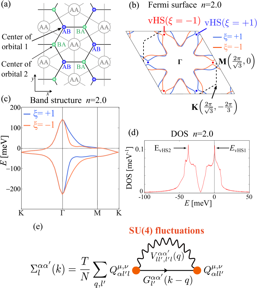
Figure 1: (a) Lattice structure of the MATBG model. Wannier orbitals 1 and 2 are centerd at AB (blue) and BA (green) sublattices, respectively. (b) FSs for $n=2.0$ and the vHS points, where orange (blue) lines and dots correspond to the valley for $\xi=+1\ (-1)$ , respectively. (c) Band structure of the MATBG model. (d) DOS for $n=2.0$, which has vHS points at $E_{\mathrm{vHS}1}$ and $E_{\mathrm{vHS}2}$. (e) Feynman diagram of the self-energy in the FLEX approximation.

Here, we analyze the following multiorbital model for MATBG studied in Ref. [60, 15]:

$$H^{0}=\sum_{{{\bm{k}}},{\alpha}{\alpha}^{\prime}l}c_{{{\bm{k}}},{\alpha}l}^{\dagger}h^{0}_{{\alpha}{\alpha}^{\prime}l}({{\bm{k}}})c_{{{\bm{k}}},{\alpha}^{\prime}l},$$ (2)

where ${{\bm{k}}}=(k_{x},k_{y})$, $l=(\rho,\xi)$, $\rho$ and $\xi$ represent spin and valley indices, respectively. Here, ${\alpha}=A\ (B)$ which represents a sublattice AB (BA) is the center of Wannier orbital 1 (2) in Fig. 1 (a). Also, the valley index $\xi=\pm 1$ correspond to the angular momentum. This model Hamiltonian is based on the first-principles tight-binding model in Ref. [60], and we modified the hopping integrals according to Ref. [15].

The Fermi surface (FS) of this model at $n=2.0$ is shown in Fig. 1 (b). Here, two FSs are labeled as $\xi=+1$ and $\xi=-1$ because $H^{0}$ is diagonal with respect to the valley. Six vHS points are shown in Fig. 1 (b). The band structure and total DOS are given in Fig. 1 (c) and Fig. 1 (d), respectively. Energy gap between the two vHS energies $E_{\mathrm{vHS1}}-E_{\mathrm{vHS2}}\sim 50$ meV corresponds to the effective bandwidth, which is consistent with the STM measurement [7].

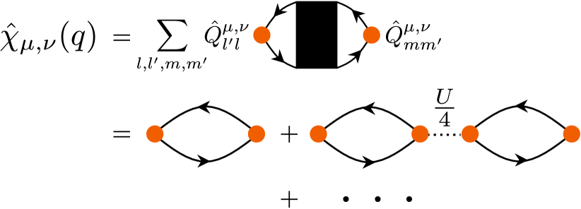
Figure 2: Diagram of the SU(4) susceptibility $\hat{\chi}_{\mu,\nu}(q)\ [(\mu,\nu)\neq(0,0)]$.

The $2\times 2$ matrix Green function with respect to the sublattices (A,B) is given as

$$\hat{G}_{l}(k)=\left[(i{\epsilon}_{n}-\mu){\hat{1}}-{\hat{h}_{l}}^{0}({{\bm{k}}})-{\hat{\Sigma}}_{l}(k)\right]^{-1},$$ (3)

where $k\equiv({{\bm{k}}},i{\epsilon}_{n})$, ${\epsilon}_{n}=(2n+1)\pi T$ and $\mu$ is the chemical potential, and ${\hat{\Sigma}}_{l}(k)$ is the self-energy.

In MATBG, the intra- and inter-valley on-site Coulomb interactions are exactly the same ($U=U^{\prime}$) [60]. Also, the inter-valley exchange interaction $J$ is very small ($J/U\ll 1$) [60, 61], therefore we set $J=0$. Then, the Coulomb interaction term is given as

$$H_{U} = \frac{U}{2}\sum_{i,{\alpha}\xi}\left(\sum_{\rho\rho^{\prime}}n_{i,{\alpha}\rho\xi}n_{i,{\alpha}\rho^{\prime}\bar{\xi}}+\sum_{\rho}n_{i,{\alpha}\rho\xi}n_{i,{\alpha}\bar{\rho}\xi}\right),$$ (4)

where $i$ is the unit cell index. $n_{i,{\alpha}\rho\xi}$ is the electron number operator with spin $\rho$ and valley $\xi$ at ${\alpha}$ spot. Using SU(4) operators in Eq. 6, $H_{U}$ is expressed as [15]

$$H_{U} = \frac{U}{16}\sum_{i,{\alpha}}\left[-\sum_{\mu,\nu}({O}^{i,{\alpha}}_{\mu,\nu})^{2}+4({O}^{i,{\alpha}}_{0,0})^{2}\right],$$ (5)

$${O}^{i,{\alpha}}_{\mu,\nu} = \sum_{ll^{\prime}}Q^{\mu,\nu}_{\alpha ll^{\prime}}c_{i,{\alpha}l}^{\dagger}c_{i,{\alpha}l^{\prime}},$$ (6)

where $\mu,\nu=0\sim 3$ and ${Q}^{\mu,\nu}_{{\alpha}ll^{\prime}}=({\hat{\sigma}}_{\mu}\otimes{\hat{\tau}}_{\nu})_{ll^{\prime}}$. Here, ${\hat{\sigma}}_{m}$ (${\hat{\tau}}_{m}$) for $m=1,2,3$ is Pauli matrix for the spin-channel with $\rho=\pm 1$ (valley-channel with $\xi=\pm 1$). ${\hat{\sigma}}_{0}$ and ${\hat{\tau}}_{0}$ are the identity matrices. The Coulomb interaction $H_{U}$ in Eq. (5) apparently possesses the SU(4) symmetry. Note that similar multipolar decomposion of the Coulomb interaction has been used in the strong heavy fermion systems in Refs. [62, 63, 64].

Here, we examine the SU(4) susceptibility given as

$$\chi_{\mu,\nu;\mu^{\prime},\nu^{\prime}}^{{\alpha}{\alpha}^{\prime}}({{\bm{q}}},i{\omega}_{l})=\int_{0}^{\beta}d\tau\langle{O}^{{\alpha}}_{\mu,\nu}({{\bm{q}}},\tau){O}^{{\alpha}^{\prime}}_{\mu^{\prime},\nu^{\prime}}(-{{\bm{q}}},0)\rangle e^{i{\omega}_{l}\tau},$$ (7)

where $q\equiv({{\bm{q}}},{\omega}_{l})$ and ${\omega}_{l}=2l\pi T$. In the present calculations, we consider only diagonal channels with respect to $(\mu,\nu)$, $\chi_{\mu,\nu;\mu,\nu}^{{\alpha}{\alpha}^{\prime}}$, because off-diagonal channels $\chi_{\mu,\nu;\mu^{\prime}\nu^{\prime}}^{{\alpha}{\alpha}^{\prime}}\ [(\mu^{\prime},\nu^{\prime})\neq(\mu,\nu)]$ are exactly zero or very small. Then, diagonal channel $\chi_{\mu,\nu}^{{\alpha}{\alpha}^{\prime}}(q)$ except for $(\mu,\nu)=(0,0)$ is expressed as

$$\begin{split}\hat{\chi}_{\mu,\nu}(q)&=\hat{\chi}^{0}_{\mu,\nu}(q)+\frac{U}{4}\hat{\chi}^{0}_{\mu,\nu}(q)\hat{\chi}^{0}_{\mu,\nu}(q)+\cdots\\ &=\hat{\chi}^{0}_{\mu,\nu}(q)\left(\hat{1}-\frac{U}{4}\hat{\chi}^{0}_{\mu,\nu}(q)\right)^{-1},\\ \end{split}$$ (8)

$$\chi^{0;{\alpha}{\alpha}^{\prime}}_{\mu,\nu}(q) =-\frac{T}{N}\sum_{k,ll^{\prime}}{Q}^{\mu,\nu}_{{\alpha}l^{\prime}l}{Q}^{\mu,\nu}_{{\alpha}^{\prime}ll^{\prime}}G_{l}^{{\alpha}{\alpha}^{\prime}}(k+q)G_{l^{\prime}}^{{\alpha}^{\prime}{\alpha}}(k).$$ (9)

Figure 2 shows the diagrammatic expression in Eq. (LABEL:eqn:chi2). Here, $\hat{\chi}_{m,0}(q)$ represents the spin susceptibility, $\hat{\chi}_{0,m}(q)$ represents the valley susceptibility, and $\hat{\chi}_{m,n}(q)$ represents the susceptibility of the ”spin-valley quadrupole order”. Also, the local charge susceptibility $\hat{\chi}_{0,0}(q)$ is expressed as

$$\hat{\chi}_{0,0}(q)=\hat{\chi}^{0}_{0,0}(q)\left(\hat{1}+\frac{3U}{4}\hat{\chi}^{0}_{0,0}(q)\right)^{-1},$$ (10)

which is suppressed by $U$.

In the FLEX approximation, the self-energy and the effective interaction are given as

$$\Sigma_{l}^{{\alpha}{\alpha}^{\prime}}(k) =\frac{T}{N}\sum_{q,l^{\prime}}G_{l^{\prime}}^{{\alpha}{\alpha}^{\prime}}(k-q)V^{{\alpha}{\alpha}^{\prime}}_{ll^{\prime},l^{\prime}l}(q),$$ (11)

$$V^{{\alpha}{\alpha}^{\prime}}_{ll^{\prime},l^{\prime}l}(q) =\left(\frac{U}{4}\right)^{2}\sum_{\begin{subarray}{c}\mu,\nu\\ \neq(0,0)\end{subarray}}Q^{\mu,\nu}_{\alpha ll^{\prime}}\chi_{\mu,\nu}^{{\alpha}{\alpha}^{\prime}}(q)Q^{\mu,\nu}_{{\alpha}^{\prime}l^{\prime}l}$$

$$\ \ \ \ \ +\left(\frac{3U}{4}\right)^{2}Q^{0,0}_{\alpha ll^{\prime}}\chi_{0,0}^{{\alpha}{\alpha}^{\prime}}(q)Q^{0,0}_{{\alpha}^{\prime}l^{\prime}l}.$$ (12)

Here, we solve Eqs. (LABEL:eqn:chi2)-(12), self-consistently. Note that the double-counting $U^{2}$ terms in Eqs. (22) are subtracted properly. In the present numerical study, we use $108\times 108\ \bm{k}$ meshes and 2048 Matsubara frequencies.

In the case of SU(4) symmetry limit, the Green function $\hat{G}_{l}(k)$ is independent of the spin and valley. Then, it is allowed to replace $\hat{G}_{l}(k)$ in Eq. (9) with $\hat{G}_{\mathrm{av}}(k)\equiv 1/4\sum_{l}\hat{G}_{l}(k)$. Therefore, the irreducible susceptibility in the SU(4) symmetry limit is approximately simplified as

$$\hat{\chi}_{\mu,\nu}^{0}(q)\approx 4\hat{\chi}_{\mathrm{av}}^{0}(q),$$ (13)

where $\chi^{0;{\alpha}{\alpha}^{\prime}}_{\mathrm{av}}(q)\equiv-\frac{T}{N}\sum_{k}G_{\mathrm{av}}^{{\alpha}{\alpha}^{\prime}}(k+q)G_{\mathrm{av}}^{{\alpha}^{\prime}{\alpha}}(k)$. Here, we used the relation $\sum_{ll^{\prime}}{Q}^{\mu,\nu}_{{\alpha}l^{\prime}l}{Q}^{\mu,\nu}_{{\alpha}ll^{\prime}}=4$ for all $\mu,\nu$. Also, the SU(4) susceptibility except for $(\mu,\nu)=(0,0)$ in Eq. (LABEL:eqn:chi2) and the self-energy in Eq. (11) in the SU(4) symmetry limit is given as

$$\hat{\chi}_{\mu,\nu}(q) \approx 4\hat{\chi}_{\mathrm{av}}(q)$$ (14)

$$\equiv 4\hat{\chi}_{\mathrm{av}}^{0}(q)\left(\hat{1}-U\hat{\chi}^{0}_{\mathrm{av}}(q)\right)^{-1},$$

$$\Sigma^{{\alpha}{\alpha}^{\prime}}(k) \approx\frac{T}{N}\sum_{q}\frac{15}{4}U^{2}G^{{\alpha}{\alpha}^{\prime}}_{\mathrm{av}}(k-q)\chi_{\mathrm{av}}^{{\alpha}{\alpha}^{\prime}}(q).$$ (15)

Eq. (15) indicates that the self-energy per orbital in this system develops easier than the systems which are considerd spin or charge fluctuations, due to the multi-channel SU(4) fluctuations.

In the presence of the off-site Coulomb interaction between $(i,{\alpha})$ and $(j,{\alpha}^{\prime})$, $v_{i{\alpha},j{\alpha}^{\prime}}$, the interaction Hamiltonian is given as

$$\begin{split}H_{v}&=\sum_{ij,{\alpha}{\alpha}^{\prime}ll^{\prime}}v_{i{\alpha},j{\alpha}^{\prime}}c_{i,{\alpha}l}^{\dagger}c_{i,{\alpha}l}c_{j,{\alpha}^{\prime}l^{\prime}}^{\dagger}c_{j,{\alpha}^{\prime}l^{\prime}}\\ &=\sum_{ij,{\alpha}{\alpha}^{\prime}}v_{i{\alpha},j{\alpha}^{\prime}}O_{0,0}^{i,\alpha}O_{0,0}^{j,\alpha^{\prime}}\end{split}$$ (16)

Then, the effect of off-site Coulomb interaction in the FLEX approximation is simply given by replacing $(3U/4)^{2}$ in Eq. (12) with $(3U/4+2v_{{\alpha}{\alpha}^{\prime}}({{\bm{q}}}))^{2}$. Here, $v_{{\alpha}{\alpha}^{\prime}}$ is the Fourier transform of $v_{i{\alpha},j{\alpha}^{\prime}}$.

Present formulation using the Coulomb interaction expressd by the SU(4) operator is equivalent to the conventional formulation using the Coulomb interaction expressed by the spin and charge channels. We explain the correspondence with the previous multiorbital FLEX approximation formalism in Appendix A.

We obtain the resistivity $\rho=1/\sigma_{xx}$ based on the Kubo formula. $\sigma_{xx}$ is given by

$$\sigma_{xx}=e^{2}\sum_{\bm{k},{\alpha}\xi}\int\frac{d\omega}{\pi}\left(-\frac{\partial f}{\partial\omega}\right)|G^{{\alpha}}_{\xi}(\bm{k},\omega)|^{2}(v^{{\alpha}}_{\xi;x}(\bm{k},\omega))^{2},$$ (17)

where $v^{{\alpha}}_{\xi;x}(\bm{k},\omega)=\partial(\epsilon^{{\alpha}}_{\xi}+\mathrm{Re}\Sigma^{{\alpha}}_{\xi}(\bm{k},\omega))/\partial k_{x}$ is the quasiparticle velocity, and $f=1/(1+e^{(\omega-\mu)/T})$. Here, ${\alpha}$ and $\xi$ denote the sublattice and valley, respectively. The self-energy $\Sigma^{{\alpha}}_{\xi}(\bm{k},\omega)$ is obtained by the analytic continuation of Eq. (11) using Pade approximation.

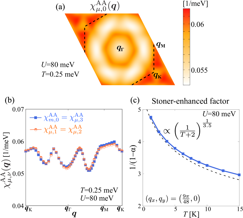
Figure 3: (a) $\bm{q}$-dependences of the spin susceptibility $\chi_{\mu,0}^{\mathrm{AA}}(\bm{q},\omega=0)$. (b) $\chi_{\mu,\nu}^{\mathrm{AA}}(\bm{q})$ obtained by the FLEX approximation. (c) $T$-dependence of the Stoner-enhanced factor ${\alpha}$.

IV numerical result

Hereafter, we mainly study the case of $n=2.0$, where the Fermi level is close to vHS energy. We consider only the on-site Coulomb interaction unless otherwise noted. Figure 3 (a) and 3 (b) show the SU(4) susceptibility $\chi_{\mu,\nu}^{\mathrm{AA}}(\bm{q})$, $\mu,\nu=0\sim 3$ [$(\mu,\nu)\neq(0,0)$]. In the present calculation, $\chi_{\mu,\nu}^{\mathrm{AA}}(\bm{q})\simeq\chi_{\mu,\nu}^{\mathrm{BB}}(\bm{q})>\chi_{\mu,\nu}^{\mathrm{AB}}(\bm{q})\simeq\chi_{\mu,\nu}^{\mathrm{BA}}(\bm{q})$ is satisfied. $\hat{\chi}_{\mu,\nu}(\bm{q})$ include not only the spin fluctuations but also, valley and valley$+$spin composite fluctuations. The fifteen components of $\hat{\chi}_{\mu,\nu}(\bm{q})$ take very similar values by reflecting the SU(4) symmetry Coulomb interaction in Eq. (5). As shown in Fig.3 (b), seven components with $(\mu,\nu)=(m,0),\ (\mu,3)$ are exactly equivalent, and eight components with $(\mu,\nu)=(\mu,1),\ (\mu,2)$ are also equivalent , where $m=1\sim 3$. In the present MATBG model given in Eq. (2), FSs are different with respect to the valley index as shown in Fig. 1(b), but the difference is very small. Therefore, the system possesses approximate SU(4) symmetry and the fifteen channels of $\hat{\chi}_{\mu,\nu}$ equally develop. Note that $\hat{\chi}_{0,0}$ is much smaller value than that in other channels ($\hat{\chi}_{0,0}\thicksim 1/10\hat{\chi}_{\mu,\nu}$). $\chi_{\mu,\nu}^{\mathrm{AA}}(\bm{q})$ develops around the nesting vector that connects the two vHS points. The Stoner factor $\alpha$ is defined as the largest eigenvalue of $U\hat{\chi}^{0}_{\mu,\nu}(\bm{q},0)/4\approx U\hat{\chi}^{0}_{\mathrm{av}}(\bm{q},0)$. It represents the SU(4) fluctuation strength. Figure 3(c) shows the $T$-dependence of the Stoner-enhanced factor. According to the spin fluctuation theory [50], the relation $1/(1-\alpha)\propto 1/T$ is satisfied due to the development of ${\alpha}$ at low temperatures, and this relation gives rise to the $T$-linear resistivity. On the other hand, in the present calculations, $\alpha\lesssim 0.8$ and $1/(1-\alpha)\propto(1/T+2)^{1/3.5}$ indicate an interesting deviation from the conventional spin fluctuation theory in MATBG.

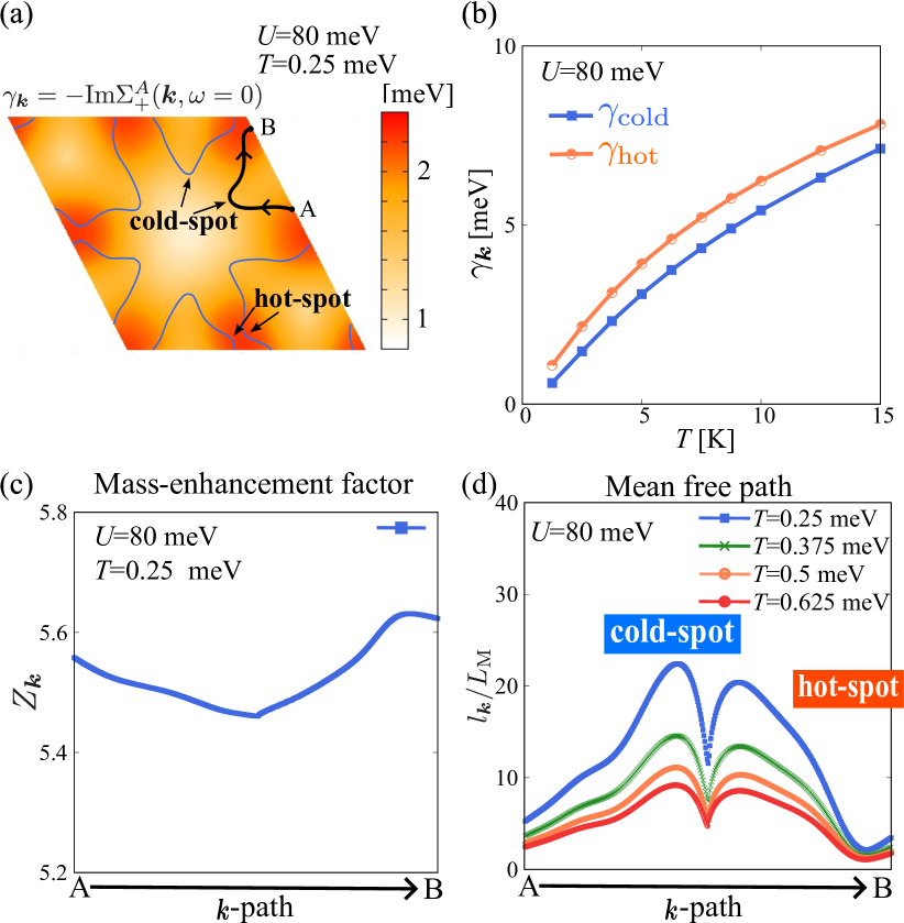
Figure 4: (a) $\bm{k}$-dependences of $\gamma_{\bm{k}}$ for ${\alpha}=A,\xi=+1$ , where blue line represents the FS. $k$-path is defined by the path from A to B on FS. (b) $T$-dependence of $\gamma_{\bm{k}}$ at cold ($\gamma_{\mathrm{cold}}$) and hot ($\gamma_{\mathrm{cold}}$) spot. $\bm{k}$-dependences of the (c) mass-enhancement factor and (d) mean free path along the $k$-path shown in (a).

Here, we show the self-energy $\Sigma^{{\alpha}}_{\xi}(\bm{k},\omega)$ obtained by the FLEX approximation. The self-energy gives the quasiparticle damping rate and the mass-enhancement factor. The quasiparticle damping rate $\gamma_{\bm{k}}$ is defined as $\gamma_{\bm{k}}=-\mathrm{Im}\Sigma^{\mathrm{A}}_{+}(\bm{k},0)\simeq-\mathrm{Im}\Sigma^{\mathrm{B}}_{+}(\bm{k},0)$. Figure 4(a) shows the $\bm{q}$-dependences of the $\gamma_{\bm{k}}$ due to the SU(4) fluctuations. There are hot (cold) spots, where $\gamma_{\bm{k}}$ takes maximum (minimum) value. The hot spots exist near the vHS points. Fig. 4(b) shows the $T$-dependence of $\gamma_{\bm{k}}$ at hot and cold spots ($\gamma_{\mathrm{hot}},\gamma_{\mathrm{cold}}$). The $T$-dependence of $\rho$ follows roughly that of $\gamma_{\mathrm{cold}}$. In our calculations, although the fluctuation per one channel is weak (${\alpha}\lesssim 0.8$) away from the SU(4) QCP, $\gamma_{\mathrm{cold}}\propto T$ is realized at low temperatures owing to the fifteen-channel SU(4) fluctuations.

The mass-enhancement factor $Z_{\bm{k}}$ and the mean free path $l_{\bm{k}}$ are given as

$$Z_{\bm{k}} = 1-\left.\frac{\partial\mathrm{Re}\Sigma_{+}^{\mathrm{A}}(\bm{k},\omega)}{\partial\omega}\right|_{\omega=0},$$ (18)

$$l_{\bm{k}} = \left\lvert\frac{\bm{v}^{{\alpha}}_{\xi}(\bm{k},0)}{\gamma_{\bm{k}}}\right\rvert,$$ (19)

where $\bm{v}^{{\alpha}}_{\xi}(\bm{k},0)$ is the quasiparticle velocity. Fig. 4(c) shows the mass-enhancement factor $Z_{\bm{k}}=m^{*}/m$ along the $\bm{k}$-path on the FS shown in Fig. 4(a), where $m$ and $m^{*}$ are the bare electron mass and the effective mass, respectively. The obtained $Z_{\bm{k}}>5$ indicates that this system is in the strongly correlated region. Fig. 4(d) shows the obtained $l_{\bm{k}}$ devided by the moiré superlattice constant $L_{\mathrm{M}}$. $l_{\bm{k}}$ on the FS is longer than $L_{\mathrm{M}}$, particularly near the cold spot. $l_{\mathrm{cold}}\sim 20L_{\mathrm{M}}$ at $T\approx 3K$. Such long $l_{\bm{k}}$ indicates that the Fermi-liquid picture holds well. Thus, in this system, the Fermi liquid state with strong correlation is realized.

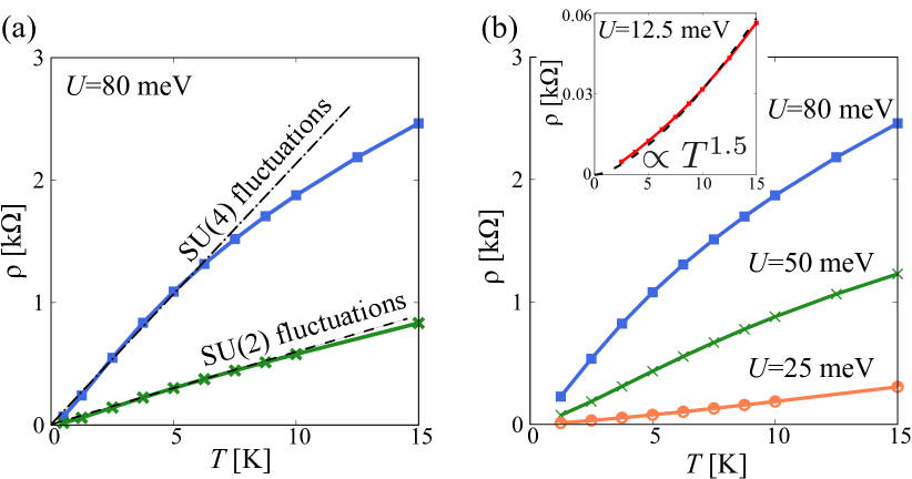
Figure 5: (a) $T$-dependence of $\rho$ obtained by FLEX approximation with SU(4) fluctuations and, that with SU(2) fluctuations for $U=80$ mev. (b) $T$-dependence of $\rho$ for $U=12.5,25,50,80$ mev.

Figure 5(a) shows the resistivity $\rho$ obtained by the FLEX approximation (blue line) due to the SU(4) fluctuations . $\rho\propto T$ is satisfied at low temperatures, which is quantitatively consistent with experimental results in Refs. [38, 39, 40]. The green line in Fig. 5(a) shows $\rho$ given by the FLEX approximation with including only spin fluctuations (SU(2) fluctuations). The $T$-linear coefficient $a=\rho/T$ due to the SU(4) fluctuations and that due to the only SU(2) fluctuations are $a\sim 0.2$ and $a\sim 0.06$, respectively. In experimental results [38, 39], the observed $T$-linear coefficient is larger than 0.1, thus our result considering the SU(4) fluctuations is consistent with the observations. On the other hand, the $T$-linear coefficient $a$ due to only the SU(2) fluctuations is very small. Therefore, the fifteen-channel SU(4) fluctuations are significant for the large $a$. We stress that the power $m$ in $\rho=aT^{m}$ decreases less than 1 at high temperature. This behavior is consistent with some experimental results [38, 39, 40], and realized in previous theoretical study based on the FLEX approximation [33, 37]. Fig. 5(b) shows the obtained $U$-dependence of $\rho$. The power $m$ increases as the Coulomb interaction becomes weak. This behavior indicates that the system approaches the Fermi liquid state ($\rho\propto T^{2}$) as $U\rightarrow 0$. Thus, the $T$-linear resistivity originates from the strong electron-electron correlation effect. Here, the power $m$ is smaller than 1.5 even when $U=12.5$ meV. As we discuss in the Appendix B, the power $m$ is smaller than 2 when the vHS points near the FS even when $U\ll W_{\mathrm{band}}$.

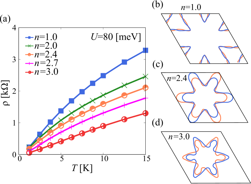
Figure 6: (a) $T$-dependence of $\rho$ for $n=1.0-3.0$. (b)-(d) FSs for $n=1.0,2.4$ and $3.0$, respectively.

Figure 6 shows the filling dependence of $\rho$, and the FSs for $n=1.0,2.4$ and $3.0$. The relation $\rho\propto T$ is satisfied in the various filling. The fifteen-channel SU(4) fluctuations originate from the (approximate) SU(4) symmetry which the system possesses by nature in MATBG. Thus, the SU(4) fluctuations easily develop even away from vHS filling, and therefore $\rho\propto T$ is realized in wide $n$ range. Experimentally, $T$-linear resistivity is observed in wide $n$ range [38, 39, 40]. Thus, our results are consistent with experiments. The $T$-linear resistivity realized in wide $n$ range suggests that the SU(4) fluctuations universally develop and non-Fermi liquid behavior in MATBG is mainly derived from the SU(4) fluctuations. The coefficient $a=\rho/T$ for $n=1.0$ is largest in $n=1.0-3.0$. This filling dependence of the coefficient $a$ is similarly observed in experiments [38, 39, 40]. The $n$-dependence of the $\gamma_{\mathrm{cold}}$ is shown in Appendix C. The obtained $\gamma_{\mathrm{cold}}$ is largest for $n=1.0$ due to the good nesting of the FS as shown in Fig. 6(b).

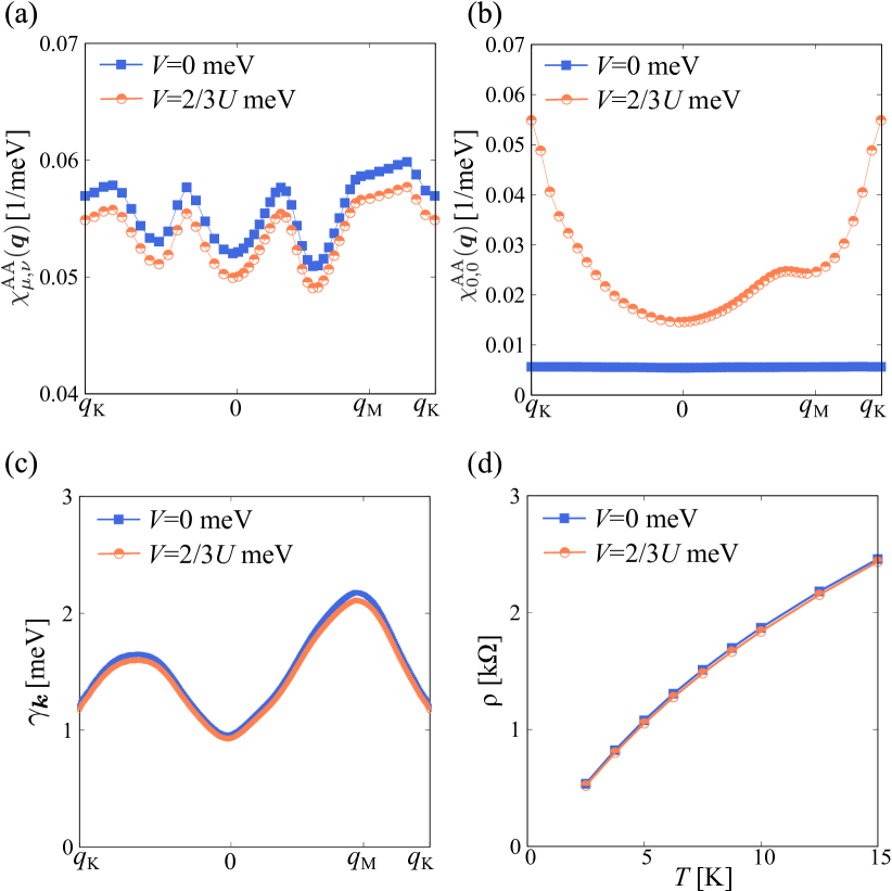
Figure 7: $\bm{q}$-dependences of (a) $\chi_{\mu,\nu}^{\mathrm{AA}}(\bm{q})$ except for $(\mu,\nu)=(0,0)$, and (b) $\chi_{0,0}^{\mathrm{AA}}(\bm{q})$ for $V=0$ (blue line) and $V_{1}=2/3U$ (orange line). (c) $\bm{k}$-dependences of $\gamma_{\bm{k}}$. (d) $T$-dependence of $\rho$.

Here, we discuss the effect of the off-site Coulomb interaction based on the Kang-Vafek model [65]. We introduce the nearest-neighbor ($V_{1}$), next nearest-neighbor ($V_{2}$), and the third next nearest-neighbor ($V_{3}$) hopping integral into the on-site Coulomb interaction term in Eq. 12 Here, we fix $U=80\ \mathrm{meV}$, $V_{1}=2V_{2}=2V_{3}$ and $V_{1}=0$ or $V_{1}=2U/3$ The results given by the FLEX approximation for $V_{1}=0$ (blue line) and $V_{1}=2U/3$ are shown in Fig. 7. Figure 7(a) shows the SU(4) susceptibility $\chi_{\mu,\nu}^{\mathrm{AA}}(\bm{q})\ [(\mu,\nu)\neq(0,0)]$. Although $\hat{\chi}_{\mu,\nu}(\bm{q})$ are slightly suppressed by the off-site Coulomb interaction, $\hat{\chi}_{\mu,\nu}(\bm{q})$ for $V_{1}=2U/3$ are fifteen-fold degenerated and quantitatively unchanged. In contrast, $\chi_{0,0}^{AA}(\bm{q})$ shown in Fig. 7(b) is drastically changed whether $V_{1}$ is zero or nonzero, and obtained $\hat{\chi}_{0,0}(\bm{q})$ for $V_{1}=2U/3$ is same order as $\chi_{\mu,\nu}(\bm{q})$. By introducing the off-site Coulomb interactions, the local charge susceptibility is modified as

$$\hat{\chi}_{0,0}(q)=\hat{\chi}_{0,0}^{0}(q)\left[\hat{1}+\left(\frac{3U}{4}+2\hat{v}(\bm{q})\right)\hat{\chi}^{0}_{0,0}(q)\right]^{-1}.$$ (20)

Here, the formulation of $\hat{\chi}_{\mu,\nu}(q)\ [(\mu,\nu)\neq(0,0)]$ in Eq. (LABEL:eqn:chi2) is unchanged, because the susceptibility $\hat{\chi}_{\mu,\nu;\mu^{\prime},\nu^{\prime}}\ [(\mu^{\prime},\nu^{\prime})\neq(\mu,\nu)]$ is negligible. Therefore, $\hat{\chi}_{0,0}(\bm{q})$ is only enlarged by $v_{{\alpha}{\alpha}^{\prime}}$, and other channels of the susceptibilities take almost the same value. The obtained damping rate $\gamma_{\bm{k}}$ is shown in Fig. 7(c). Nevertheless $\hat{\chi}_{0,0}(\bm{q})\thicksim\hat{\chi}_{\mu,\nu}(\bm{q})$ for $V_{1}=2U/3$, $\gamma_{\bm{k}}$ is almost equivalent to that for $V_{1}=0$. This is because the contribution of $\hat{\chi}_{0,0}(\bm{q})$ to $\gamma_{\bm{k}}$ is just 1/16 of other all channels, and $\hat{\chi}_{\mu,\nu}(\bm{q})\ [(\mu,\nu)\neq(0,0)]$ is essentially independent of $V$. Consequently, the resistivity $\rho$ obtained for $V_{1}=2U/3$ is almost the same as that for $V_{1}=0$. Therefore, the present analysis based on the on-site Coulomb interaction $U$ is justified.

V summary

In this study, we demonstrated that the $T$-linear resistivity is realized by the electron-electron correlation in MATBG in the presence of the SU(4) valley+spin composite fluctuations. We calculated the self-energy by employing the FLEX approximation. The obtained self-energy takes large value due to the fifteen-fold degenerated SU(4) fluctuations. Robust $T$-linear resistivity is realized for wide ranged $n$ at low temperatures derived from the SU(4) fluctuations. Importantly, the $T$-linear resistivity is realized even when the system is far from the SU(4) QCP (${\alpha}\lesssim 0.8$ in our calculations). Then, large $T$-linear coefficient $a\equiv\rho/T$ is obtained in the present mechanism. The $T$-linear coefficient $a$ due to only the spin fluctuations is small, which is less than 1/10 of the coefficient observed in Ref. [38, 39]. Thanks to the SU(4) fluctuations, robust and large $T$-linear resistivity is observed for wide $n$ range, even away from $n_{\mathrm{vHS}}=2.0$, consistent with experiments. This result is strong evidence that the SU(4) fluctuations universally develop in MATBG.

As well as MATBG, the exotic electronic states appear in other twisted multilayer graphene. For example, non-Fermi liquid type transport phenomena [66, 67] , unconventional superconductivity [68, 67, 69] , and nematic ordere [70] has been observed in twisted double bilayer graphene (TDBG). Furthermore, in trilayer graphene, unconventional superconducting state appears [71]. The present Green function formalism in the SU(4) symmetry limit will be useful in analyzing the abovementioned problems.

VI acknowledgements

This study has been supported by Grants-in-Aid for Scientific Research from MEXT of Japan (JP18H01175, JP20K03858, JP20K22328, JP22K14003), and by the Quantum Liquid Crystal No. JP19H05825 KAKENHI on Innovative Areas from JSPS of Japan.

VII appendix A: FLEX approximation for multiorbital Hubbard models

In this Appendix, we explain another foumulation of the multiorbital FLEX approximation based on the matrix expressions of the Coulomb interaction. This method has been widely used for ruthenate [72], cobaltates [73], Fe-based superconductors [74, 75, 18], and heavy fermions [62, 63, 64]. It is confirmed that the formulation using SU(4) operator developed in the main text is equivalent with the following formulation.

The Coulomb interaction $H_{U}$ in Eq. (4) is decomposed into spin and charge channel as [16]

$$H_{U} = \frac{U}{8}\sum_{i,{\alpha}}\sum_{\{\rho\},\{\xi\}}\left[-\hat{\Gamma}^{s}_{\xi_{1}\xi_{2},\xi_{3}\xi_{4}}(\hat{\bm{{\sigma}}}\otimes\hat{\bm{{\sigma}}})_{\rho_{1}\rho_{2},\rho_{3}\rho_{4}}\right.$$ (21)

$$\left.-\hat{\Gamma}^{c}_{\xi_{1}\xi_{2},\xi_{3}\xi_{4}}({\hat{\sigma}}^{0}\otimes{\hat{\sigma}}^{0})_{\rho_{1}\rho_{2},\rho_{3}\rho_{4}}\right]$$

$$\times c_{i,{\alpha}\rho_{1}\xi_{1}}^{\dagger}c_{i,{\alpha}\rho_{2}\xi_{2}}c_{i,{\alpha}\rho_{4}\xi_{4}}^{\dagger}c_{i,{\alpha}\rho_{3}\xi_{3}},$$

where $\hat{\bm{{\sigma}}}$ and $\hat{{\sigma}}^{0}$ are Pauli matrix and identity matrix, respectively and $\xi_{i}$ is valley index. Here, $\Gamma^{s}_{\xi_{1}\xi_{2},\xi_{3}\xi_{4}}=U$ for $\xi_{1}=\xi_{2}=\xi_{3}=\xi_{4}$ and $\xi_{1}=\xi_{3}=-\xi_{2}=-\xi_{4}$, and $\Gamma^{s}=0$ for others. Also, $\Gamma^{c}_{\xi_{1}\xi_{2},\xi_{3}\xi_{4}}=-U$ for $\xi_{1}=\xi_{2}=\xi_{3}=\xi_{4}$, $\Gamma^{c}=-2U$ for $\xi_{1}=\xi_{2}=-\xi_{3}=-\xi_{4}$, $\Gamma^{c}=U$ for $\xi_{1}=\xi_{3}=-\xi_{2}=-\xi_{4}$, and $\Gamma^{c}=0$ for others. The self-energy in the FLEX calculation is given as

$$\Sigma_{{\alpha}{\alpha}^{\prime}\xi}(k) =\frac{T}{N}\sum_{q}G_{{\alpha}{\alpha}^{\prime}\xi}(k-q)V_{{\alpha}\xi\xi^{\prime},{\alpha}^{\prime}\xi^{\prime}\xi}(q),$$ (22)

$$V_{{\alpha}\xi\xi^{\prime},{\alpha}^{\prime}\xi^{\prime}\xi}(q) =\frac{U^{2}}{2}(3{\hat{\Gamma}}^{s}{\hat{\chi}}^{s}_{{\alpha}{\alpha}^{\prime}}(q){\hat{\Gamma}}^{s}$$

$$\ \ \ \ \ \ \ \ \ \ +{\hat{\Gamma}}^{c}{\hat{\chi}}^{c}_{{\alpha}{\alpha}^{\prime}}(q){\hat{\Gamma}}^{c})_{\xi\xi^{\prime},\xi^{\prime}\xi},$$ (23)

$${\chi}^{0}_{{\alpha}\xi_{1}\xi_{2},{\alpha}^{\prime}\xi_{3}\xi_{4}}(q)$$

$$=-\frac{T}{N}\sum_{k} G_{{\alpha}{\alpha}^{\prime}\xi_{1}}(k+q)G_{{\alpha}^{\prime}{\alpha}\xi_{2}}(k)\delta_{\xi_{1},\xi_{3}}\delta_{\xi_{2},\xi_{4}},$$ (24)

$${\hat{\chi}}^{s(c)}(q) ={\hat{\chi}}^{0}(q)({\hat{1}}-{\hat{\Gamma}}^{s(c)}{\hat{\chi}}^{0}(q))^{-1},$$ (25)

where $\hat{\chi}^{s(c)}$ is the spin (charge) susceptibility. The self-energy in the FLEX approximation is given by solving Eqs. (22)-(25) self-consistently. The coefficients for the self-energy originated from the spin fluctuations and the charge fluctuation are 3/2 and 1/2, respectively. The spin (charge) Stoner factor ${\alpha}^{s(c)}$ is defined as the maximum eigenvalue of ${\hat{\Gamma}}^{s(c)}\hat{\chi}^{s(c)}_{{\alpha}{\alpha}^{\prime}}$. ${\alpha}^{s}$ and ${\alpha}^{c}$ are exactly equivalent due to the relation $U=U^{\prime}$.

In the presence of the off-site Coulomb interaction between $(i,{\alpha})$ and $(j,{\alpha}^{\prime})$, $v_{i{\alpha},j{\alpha}^{\prime}}$ given as Eq. (16), the effect of off-site Coulomb interaction in the FLEX approximation is simply given by replacing ${\hat{\Gamma}}^{c}$ with ${\hat{\Gamma}}^{c}+v_{{\alpha}{\alpha}^{\prime}}({{\bm{q}}})\delta_{\xi_{1},\xi_{2}}\delta_{\xi_{3},\xi_{4}}$ in Eqs. (23) and (25). Here, $v_{{\alpha}{\alpha}^{\prime}}({{\bm{q}}})$ is the Fourier transform of $v_{i{\alpha},j{\alpha}^{\prime}}$.

The SU(4) susceptibility in Eq. (LABEL:eqn:chi2) can be expanded by the spin and charge susceptibilities in Eq. (25) as

$$\begin{split}\chi_{\mu,\nu}^{{\alpha}{\alpha}^{\prime}}({{\bm{q}}},i{\omega}_{l})&=\int_{0}^{\beta}d\tau\langle O_{\mu,\nu}^{{\alpha}}({{\bm{q}}},\tau)O_{\mu,\nu}^{{\alpha}^{\prime}}(-{{\bm{q}}},0)\rangle e^{i{\omega}_{l}\tau}\\ &=\sum_{l_{1}l_{2}l_{3}l_{4}}Q^{\mu,\nu}_{{\alpha}l_{1}l_{2}}\chi_{{\alpha}l_{1}l_{2},{\alpha}^{\prime}l_{3}l_{4}}(q)Q^{\mu,\nu}_{{\alpha}^{\prime}l_{3}l_{4}},\end{split}$$ (26)

where ${Q}^{\mu,\nu}_{{\alpha}ll^{\prime}}=({\hat{\sigma}}_{\mu}\otimes{\hat{\tau}}_{\nu})_{ll^{\prime}}$ and $l_{i}=(\rho_{i},\xi_{i})$. The general susceptibility in the right-hand-side of Eq. (26) is given as

$$\chi_{{\alpha}l_{1}l_{2},{\alpha}^{\prime}l_{3}l_{4}}(q) =\frac{1}{2}\chi_{{\alpha}\xi_{1}\xi_{2},{\alpha}^{\prime}\xi_{3}\xi_{3}}^{s}(q)(\hat{\bm{{\sigma}}}\otimes\hat{\bm{{\sigma}}})_{\rho_{1}\rho_{2},\rho_{3}\rho_{4}}$$

$$+\frac{1}{2}\chi_{{\alpha}\xi_{1}\xi_{2},{\alpha}^{\prime}\xi_{3}\xi_{3}}^{c}(q)({\hat{\sigma}}^{0}\otimes{\hat{\sigma}}^{0})_{\rho_{1}\rho_{2},\rho_{3}\rho_{4}}.$$ (27)

This conventional formalism used in Refs. [72, 73, 74, 75, 18, 62, 63, 64] is exactly equivalent with the SU(4) operator formalism explained in the main text.

VIII appendix B: resistivity within the second-order perturbation theory

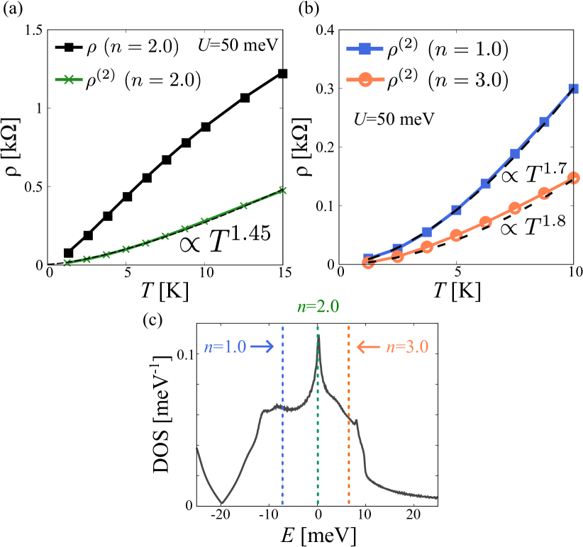
Figure 8: (a) $T$-dependence of $\rho$ obtained by the FLEX approximation with full-order (black line) and that in the self-consistent second-order perturbation theory (green line) for $n=2.0$. (b) $T$-dependence of $\rho$ obtained by the self-consistent second-order perturbation theory for $n=1.0$ (blue line) and $n=3.0$ (orange line). (c) The total DOS, broken lines with blue, green and orange represent the Fermi energy for $n=1.0$, $n=2.0$ and $n=3.0$, respectively.

Here, we discuss the important effect of vHS points on the resistivity $\rho$ in the weak coupling region. In the main text, the obtained power $m$ in $\rho=aT^{m}$ is smaller than about 1.5 for $n=2.0$, even in the case of very weak on-site Coulomb interaction $U$. This result is inconsistent with the expected behavior that the Fermi liquid behavior $\rho\propto T^{2}$ is obtained for the limit $U\rightarrow 0$. To understand this inconsistence, we calculate the resistivity $\rho^{(2)}$, which is given by the self-consistent second-order perturbation theory with respect to $U$. Figure 8 (a) shows $\rho$ with full order (black line) and within second-order perturbation theory (green line) with respect to $U$, and (b) shows $\rho^{(2)}$ for $n=1.0$ (blue line) and $n=3.0$ (orange line). We set $U=50$ meV in Fig. 8. The obtained power $m$ in $\rho^{(2)}=aT^{m}$ for $n=2.0$ is $m=1.45$, and this is almost same with $m$ for $U=12.5$ meV in Fig. 5. In contrast, the power $m$ in $\rho^{(2)}$ for $n=1.0,3.0$ are close to 2. This results suggest that the power $m$ is enhanced by the effect of vHS points and $T$-linear resistivity is easily realized near the vHS points.

IX Appendix C: Filling dependence of $\gamma_{\mathrm{cold}}$

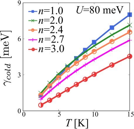
Figure 9: (a) $T$-dependence of the damping rate at cold spot, $\gamma_{\mathrm{cold}}$ for $n=1.0-3.0$.

Figure 9 shows the filling dependence of $\gamma_{\mathrm{cold}}$ for $n=1.0-3.0$. $\gamma_{\mathrm{cold}}$ for $n=2.0-3.0$ get small as the filling is far from $n_{\mathrm{VHS}}\simeq 2.0$. Unexpectedely, the obtained $\gamma_{\mathrm{cold}}$ for $n=1.0$ at $T\gtrsim 10$K takes larger value than it for $n=2.0$ in our calculation. The reason is that the nesting condition on the FS for $n=1.0$ in Fig. 6 (b) is better than that for $n=2.0$ in Fig. 1 (b). Consequently, SU(4) susceptibilities for $n=1.0$ are higher than that for $n=2.0$ by reflecting the good nesting condition of the FS. (FS for $n=1.0$ is shown in Fig. 6 (b).) Thus, $\gamma_{\mathrm{cold}}$ for $n=1.0$ takes the largest value due to the stronger nesting effect, which exceeds the effect of the reduced DOS.

References

- [1] Y. Cao, V. Fatemi, S. Fang, K. Watanabe, T. Taniguchi, E. Kaxiras, and P. Jarillo-Herrero, Unconventional superconductivity in magic-angle graphene superlattices, Nature 556, 43 (2018).
- [2] Y. Cao, V. Fatemi, A. Demir, S. Fang, S. L. Tomarken, J. Y. Luo, J. D. Sanchez-Yamagishi, K. Watanabe, T. Taniguchi, E. Kaxiras, R. C. Ashoori, and P. Jarillo-Herrero, Correlated insulator behaviour at half-filling in magic-angle graphene superlattices, Nature 556, 80 (2018).
- [3] M. Yankowitz, S. Chen, H. Polshyn, Y. Zhang, K. Watanabe, T. Taniguchi, D. Graf, A. F. Young, and C. R. Dean, Tuning superconductivity in twisted bilayer graphene, Science 363, 1059 (2019).
- [4] X. Lu, P. Stepanov, W. Yang, M. Xie, M. A. Aamir, I. Das, C. Urgell, K. Watanabe, T. Taniguchi, G. Zhang, A. Bachtold, A. H. MacDonald, and D. K. Efetov, Superconductors, orbital magnets and correlated states in magic-angle bilayer graphene, Nature 574, 653 (2019).
- [5] A. L. Sharpe, C. L. Tschirhart, H. Polshyn, Y. Zhang, J.Zhu, K. Watanabe, T. Taniguchi, L. Balents, and A. F. Young, Emergent ferromagnetism near three-quarters filling in twisted bilayer graphene, Science 365, 605 (2019).
- [6] M. Serlin, C. L. Tschirhart, H. Polshyn, Y. Zhang, J. Zhu, K. Watanabe, T. Taniguchi, L. Balents, A. F. Young, Intrinsic quantized anomalous Hall effect in a moiré heterostructure, Science 367, 900 (2020).
- [7] A. Kerelsky, L. McGilly, D. M. Kennes, L. Xian, M. Yankowitz, S. Chen, K. Watanabe, T. Taniguchi, J. Hone, C. Dean, A. Rubio, and A. N. Pasupathy, Maximized electron interactions at the magic angle in twisted bilayer graphene, Nature 572, 95 (2019).
- [8] Y. Choi, J. Kemmer, Y. Peng, A. Thomson, H. Arora, R. Polski, Y. Zhang, H. Ren, J. Alicea, G. Refael, F. von Oppen, K. Watanabe, T. Taniguchi, and S. Nadj-Perge, Electronic correlations in twisted bilayer graphene near the magic angle, Nat. Phys. 15, 1174 (2019).
- [9] Y. Jiang, X. Lai, K. Watanabe, T. Taniguchi, K. Haule, J. Mao, and E. Y. Andrei, Charge order and broken rotational symmetry in magic-angle twisted bilayer graphene, Nature 573, 91 (2019).
- [10] Y. Cao, D. R. Legrain, J. M. Park, F. N. Yuan, K. Watanabe, T. Taniguchi, R. M. Fernandes, L. Fu, and P. J. Herrero, Nematicity and competing orders in superconducting magic-angle graphene, Science 372, 264 (2021).
- [11] K. P. Nuckolls, R. L. Lee1, M. Oh, D. Wong1, T. Soejima, J. P. Hong1, D. Călugăru, J. Herzog-Arbeitman, B. A. Bernevig, K. Watanabe, T. Taniguchi, N. Regnault, M. P. Zaletel, and A. Yazdani, Quantum textures of the many-body wavefunctions in magic-angle graphene, Nature 620, 525 (2023).
- [12] H. Kim, Y. Choi, ÁE Lantagne-Hurtubise, C. Lewandowski, A. Thomson, L. Kong, H. Zhou, E. Baum, Y. Zhang, L. Holleis, K. Watanabe, T. Taniguchi, A. F. Young, J. Alicea, and Stevan Nadj-Perge, Imaging inter-valley coherent order in magic-angle twisted trilayer graphene, Nature 623, 942 (2023).
- [13] H. Isobe, N. F. Q. Yuan, and L. Fu, Unconventional Superconductivity and Density Waves in Twisted Bilayer Graphene, Phys. Rev. X 8, 041041 (2018).
- [14] D. V. Chichinadze, L. Classen, and A. V. Chubukov, Nematic superconductivity in twisted bilayer graphene, Phys. Rev. B 101, 224513 (2020).
- [15] S. Onari and H. Kontani, SU(4) Valley + Spin Fluctuation Interference Mechanism for Nematic Order in Magic-Angle Twisted Bilayer Graphene: The Impact of Vertex Corrections, Phys. Rev. Lett. 128, 066401 (2022).
- [16] H. Kontani, R. Tazai, Y. Yamakawa, and S. Onari, Unconventional density waves and superconductivities in Fe-based superconductors and other strongly correlated electron systems, Adv. Phys. 70, 355 (2021).
- [17] R. Tazai, S. Matsubara, Y. Yamakawa, S. Onari, and H. Kontani, Rigorous formalism for unconventional symmetry breaking in Fermi liquid theory and its application to nematicity in FeSe, Phys. Rev. B 107, 035137 (2023).
- [18] S. Onari and H. Kontani, Self-consistent Vertex Correction Analysis for Iron-based Superconductors: Mechanism of Coulomb Interaction-Driven Orbital Fluctuations, Phys. Rev. Lett. 109, 137001 (2012).
- [19] S. Onari, Y. Yamakawa, and H. Kontani, Sign-Reversing Orbital Polarization in the Nematic Phase of FeSe due to the Symmetry Breaking in the Self-Energy, Phys. Rev. Lett. 116, 227001 (2016).
- [20] Y. Yamakawa, S. Onari, and H. Kontani, Nematicity and Magnetism in FeSe and Other Families of Fe-Based Superconductors, Phys. Rev. X 6, 021032 (2016).
- [21] S. Onari and H. Kontani, rigin of diverse nematic orders in Fe-based superconductors: rotated nematicity in Fe2As2 , Phys. Rev. B 100, 020507(R) (2019).
- [22] R. Q. Xing, L. Classen, A. V. Chubukov, Orbital order in FeSe: The case for vertex renormalization, Phys. Rev. B 98, 041108(R) (2018).
- [23] A. V. Chubukov, M. Khodas, and R. M. Fernandes, Magnetism, Superconductivity, and Spontaneous Orbital Order in Iron-Based Superconductors: Which Comes First and Why?, Phys. Rev. X 6, 041045 (2016).
- [24] M. Tsuchiizu, K. Kawaguchi, Y. Yamakawa, and H. Kontani, Multistage electronic nematic transitions in cuprate superconductors: A functional-renormalization-group analysis, Phys. Rev. B 97, 165131 (2018).
- [25] S. Onari and H. Kontani, Strong Bond-Order Instability with Three-Dimensional Nature in Infinite-Layer Nickelates due to Non-Local Quantum Interference Mechanism, arXiv:2212.13784 (2022).
- [26] R. Tazai, Y. Yamakawa, S. Onari, and H. Kontani, Mechanism of exotic density-wave and beyond-Migdal unconventional superconductivity in kagome metal , Sci. Adv. 8, eabl4108 (2022).
- [27] R. Tazai, Y. Yamakawa, and H. Kontani, Charge-loop current order and Z3 nematicity mediated by bond-order fluctuations in kagome metals, Nat. Commun. 14, 7845 (2023).
- [28] R. Tazai, Y. Yamakawa, and H. Kontani, Drastic magnetic-field-induced chiral current order and emergent current-bond-field interplay in kagome metals, accepted for publication in Proceedings of the National Academy of Sciences (PNAS) (available at https://arxiv.org/abs/2303.00623).
- [29] M. Tsuchiizu, Y. Ohno, S. Onari, and H. Kontani, Orbital Nematic Instability in the Two-Orbital Hubbard Model: Renormalization-Group + Constrained RPA Analysis, Phys. Rev. Lett. 111, 057003 (2013).
- [30] E. H. Hwang and S. D. Sarma, Acoustic phonon scattering limited carrier mobility in two-dimensional extrinsic graphene, Phys. Rev. B 77, 115449 (2008).
- [31] F. Wu, E. Hwang, and S. D. Sarma, Phonon-induced giant linear-in-T resistivity in magic angle twisted bilayer graphene: Ordinary strangeness and exotic superconductivity, Phys. Rev. B 99, 165112 (2019).
- [32] R. M. Fernandes and J. W. F. Venderbos, Nematicity with a twist: Rotational symmetry breaking in a moiré superlattice, Sci. Adv. 6, 8834 (2020).
- [33] H. Kontani, K. Kanki, and K. Ueda, Hall effect and resistivity in high- superconductors: The conserving approximation, Phys. Rev. B 59, 14723 (1999).
- [34] Hiroshi Kontani, General formula for the magnetoresistance on the basis of Fermi liquid theory, Phys. Rev. B 64, 054413 (2001).
- [35] H. Kontani, Magnetoresistance in High- Superconductors: The Role of Vertex Corrections, J. Phys. Soc. Jpn. 70, 1873 (2001).
- [36] Hiroshi Kontani, Nernst Coefficient and Magnetoresistance in High- Superconductors: The Role of Superconducting Fluctuations, Phys. Rev. Lett. 89, 237003 (2002).
- [37] H. Kontani, Anomalous transport phenomena in Fermi liquids with strong magnetic fluctuations, Rep. Prog. Phys. 71, 026501 (2008).
- [38] A. Jaoui, I. Das, G. D. Battista, J. Díez-Mérida, X. Lu, K. Watanabe, T. Taniguchi, H. Ishizuka, L. Levitov, and D. K. Efetov, Quantum critical behaviour in magic-angle twisted bilayer graphene, Nat. Phys. 18, 633 (2022).
- [39] H. Polshyn, M. Yankowitz, S. Chen, Y. Zhang, K. Watanabe, T. Taniguchi, C. R. Dean, and A. F. Young, Large linear-in-temperature resistivity in twisted bilayer graphene, Nat. Phys. 15, 1011 (2019).
- [40] J. M. Park, Y. Cao, K. Watanabe, T. Taniguchi, and P. Jarillo-Herrero, Flavour Hund’s coupling, Chern gaps and charge diffusivity in moiré graphene, Nat. Phys. 592, 43 (2021).
- [41] R. Lyu, Z. Tuchfeld, N. Verma, H. Tian, K. Watanabe, T. Taniguchi, C. Ning Lau, M. Randeria, and M. Bockrath, Strange metal behavior of the Hall angle in twisted bilayer graphene, Phys. Rev. B 103, 245424 (2021).
- [42] T. Nakazima, H. Yoshizawa, and Y. Ueda, -site Randomness Effect on Structural and Physical Properties of Ba-based Perovskite Manganites, J. Phys. Soc. Jpn. 73, 5 (2004).
- [43] Y. Nakajima Y. Nakajima, H. Shishido, H. Nakai, T. Shibauchi, K. Behnia, K. Izawa, M. Hedo, Y. Uwatoko, T. Matsumoto, R. Settai, Y. Onuki, H. Kontani, and Y. Matsuda, Non-Fermi Liquid Behavior in the Magnetotransport of CeIn5 (: Co and Rh): Striking Similarity between Quasi Two-Dimensional Heavy Fermion and High- Cuprates, J. Phys. Soc. Jpn. 76, 024703 (2007).
- [44] J. P. Sun, G. Z. Ye, P. Shahi, J.-Q. Yan, K. Matsuura, H. Kontani, G. M. Zhang, Q. Zhou, B. C. Sales, T. Shibauchi, Y. Uwatoko, D. J. Singh, and J.-G. Cheng, High- Superconductivity in FeSe at High Pressure: Dominant Hole Carriers and Enhanced Spin Fluctuations, Phys. Rev. Lett. 118, 147004 (2017).
- [45] W. K. Huang, S. Hosoi, M. ulo, S. Kasahara, Y. Sato, K. Matsuura, Y. Mizukami, M. Berben, N. E. Hussey, H. Kontani, T. Shibauchi, and Y. Matsuda, Non-Fermi liquid transport in the vicinity of the nematic quantum critical point of superconducting , Phys. Rev. Res. 2, 033367 (2020).
- [46] D. Li, B. Y. Wang, K. Lee, S. P. Harvey, M. Osada, B. H. Goodge, L. F. Kourkoutis, and H. Y. Hwang, Superconducting Dome in Infinite Layer Films, Phys. Rev. Lett. 125, 027001 (2020).
- [47] K. Lee, B. Y. Wang, M. Osada, B. H. Goodge, T. C. Wang, Y. Lee, S. Harvey, W. J. Kim, Y. Yu, C. Murthy, S. Raghu, L. F. Kourkoutis, H. Y. Hwang, Character of the ”normal state” of the nickelate superconductors, arXiv:2203.02580 (2022).
- [48] H. Takagi, T. Ido, S. Ishibashi, M. Uota, S. Uchida, and Y. Tokura, Superconductor-to-nonsuperconductor transition in as investigated by transport and magnetic measurements, Phys. Rev. B 40, 2254 (1989).
- [49] R. Daou, N. Doiron-Leyraud, D. LeBoeuf, S.Y. Li, F. Lalibertè, O. Cyr-Choinière, Y.J. Jo, L. Balicas, J.-Q. Yan, J.-S. Zhou,J.B. Goodenough, and L. Taillefer, Linear temperature dependence of resistivity and change in the Fermi surface at the pseudogap critical point of a high-Tc superconductor, Nat. Phys. 5, 31 (2009).
- [50] T. Moriya and K. Ueda, Spin fluctuations and high temperature superconductivity, Adv. Phys. 49, 555 (2000).
- [51] J. A. Hertz, Quantum critical phenomena, Phys. Rev. B 14, 1165 (1976).
- [52] A. J. Millis, Effect of a nonzero temperature on quantum critical points in itinerant fermion systems, Phys. Rev. B 48, 7183 (1993).
- [53] R. Hlubina and T. M. Rice, Resistivity as a function of temperature for models with hot spots on the Fermi surface, Phys. Rev. B 51, 9253 (1995).
- [54] B. P. Stojkovic and D. Pines, Theory of the longitudinal and Hall conductivities of the cuprate superconductors, Phys. Rev. B 55, 8576 (1997).
- [55] A. Abanov, A. V. Chubukov, J. Schmalian, Quantum critical theory of the spin-fermionmodel and its application to cuprates: Normal state analysis, Adv. Phys. 52, 119 (2003).
- [56] N. E. Bickers and S. R. White, Conserving approximations for strongly fluctuating electron systems. II. Numerical results and parquet extension, Phys. Rev. B 43, 8044 (1991).
- [57] T. Dahm and L. Tewordt, Physical quantities in nearly antiferromagnetic and superconducting states of the two-dimensional Hubbard model and comparison with cuprate superconductors, Phys. Rev. B 52, 1297 (1995).
- [58] T. Takimoto and T. Moriya, Theory of Spin Fluctuation-Induced Superconductivity Based on a d- p Model. II. -Superconducting State-, J. Phys. Soc. Jpn. 67, 3570 (1994).
- [59] H. Kontani and M. Ohno, Effect of a nonmagnetic impurity in a nearly antiferromagnetic Fermi liquid: Magnetic correlations and transport phenomena, Phys. Rev. B 74, 014406 (2006).
- [60] M. Koshino, N. F. Q. Yuan, T. Koretsune, M. Ochi, K. Kuroki, and L. Fu, Maximally Localized Wannier Orbitals and the Extended Hubbard Model for Twisted Bilayer Graphene, Phys. Rev. X 8, 031087 (2018).
- [61] M. J. Klug, Charge order and Mott insulating ground states in small-angle twisted bilayer graphene, New J. Phys. 22, 073016 (2020).
- [62] R. Tazai and H. Kontani, Fully gapped -wave superconductivity enhanced by magnetic criticality in heavy-fermion systems, Phys. Rev. B 98, 205107 (2018).
- [63] R. Tazai and H. Kontani, Multipole fluctuation theory for heavy fermion systems: Application to multipole orders in , Phys. Rev. B 100, 241103(R) (2019).
- [64] R. Tazai and H. Kontani, Hexadecapole Fluctuation Mechanism for -wave Heavy Fermion Superconductor : Interplay between Intra- and Inter-Orbital Cooper Pairs, J. Phys. Soc. Jpn. 88, 063701 (2019).
- [65] J. Kang and O. Vafek, Strong Coupling Phases of Partially Filled Twisted Bilayer Graphene Narrow Bands, Phys. Rev. Lett. 122, 246401 (2019).
- [66] G. W. Burg, J. Zhu, T. Taniguchi, K. Watanabe, A. H. MacDonald, and E. Tutuc, Correlated Insulating States in Twisted Double Bilayer Graphene, Phys. Rev. Lett. 123, 197702 (2019).
- [67] X. Liu, Z. Hao, E. Khalaf, J. Y. Lee, Y. Ronen, H. Yoo, D. H. Najafabadi, K. Watanabe, T. Taniguchi, A. Vishwanath, and P. Kim, Tunable spin-polarized correlated states in twisted double bilayer graphene, Nature 583, 221 (2019).
- [68] C. Shen, Y. Chu, Q. Wu, N. Li, S. Wang, Y Zhao, J. Tang, J. Liu, J. Tian, K. Watanabe, T. Taniguchi, R. Yang, Z. Y. Meng, D. Shi, O. V. Yazyev, and G. Zhang, Correlated states in twisted double bilayer graphene, Nat. Phys. 16, 520 (2020).
- [69] M. He, Y. Li, J. Cai, Y. Liu, K. Watanabe, T. Taniguchi, X. Xu, and M. Yankowitz, Symmetry breaking in twisted double bilayer graphene, Nat. Phys. 17, 26 (2021).
- [70] R. Samajdar, M. S Scheurer, S. Turkel, C. Rubio-Verdú, A. N Pasupathy, J. W F Venderbos, and R. M Fernandes, Electric-field-tunable electronic nematic order in twisted double-bilayer graphene, 2D Mater. 8, 034005 (2021).
- [71] H. Zhou1, T. Xie, T. Taniguchi, K. Watanabe, and A. F. Young, Superconductivity in rhombohedral trilayer graphene, Nature 598, 434 (2021).
- [72] T. Takimoto, Orbital fluctuation-induced triplet superconductivity: Mechanism of superconductivity in Phys. Rev. B 62, R14641(R) (2000).
- [73] K. Yada and H. kontani, Origin of Weak Pseudogap Behaviors in : Absence of Small Hole Pockets, J. Phys. Soc. Jpn. 74, 2161 (2005).
- [74] K. Kuroki, S. Onari, R. Arita, H. Usui, Y. Tanaka, H. Kontani, and H. Aoki, Unconventional Pairing Originating from the Disconnected Fermi Surfaces of Superconducting , Phys. Rev. Lett. 101, 087004 (2008).
- [75] H. Kontani and S. Onari, Orbital-Fluctuation-Mediated Superconductivity in Iron Pnictides: Analysis of the Five-Orbital Hubbard-Holstein Model, Phys. Rev. Lett. 104, 157001 (2010).