An extended asymmetric sigmoid with Perceptron(SIGTRON) for imbalanced linear classification

Abstract

This article presents a new polynomial parameterized sigmoid called SIGTRON, which is an extended asymmetric sigmoid with Perceptron, and its companion convex model called SIGTRON-imbalanced classification (SIC) model that employs a virtual SIGTRON-induced convex loss function. In contrast to the conventional $\pi$-weighted cost-sensitive learning model, the SIC model does not have an external $\pi$-weight on the loss function but has internal parameters in the virtual SIGTRON-induced loss function. As a consequence, when the given training dataset is close to the well-balanced condition, we show that the proposed SIC model is more adaptive to variations of the dataset, such as the inconsistency of the scale-class-imbalance ratio between the training and test datasets. This adaptation is achieved by creating a skewed hyperplane equation. Additionally, we present a quasi-Newton optimization(L-BFGS) framework for the virtual convex loss by developing an interval-based bisection line search. Empirically, we have observed that the proposed approach outperforms $\pi$-weighted convex focal loss and balanced classifier LIBLINEAR(logistic regression, SVM, and L2SVM) in terms of test classification accuracy with $51$ two-class and $67$ multi-class datasets. In binary classification problems, where the scale-class-imbalance ratio of the training dataset is not significant but the inconsistency exists, a group of SIC models with the best test accuracy for each dataset (TOP$1$) outperforms LIBSVM(C-SVC with RBF kernel), a well-known kernel-based classifier.

I Introduction

Learning a hyperplane from the given training dataset ${\cal D}=\{(x_{l},y_{l})\in{\mathbb{R}}^{s}\times\{-1,+1\}\;|\;l=1,2,\cdots,d\}$ is the most fundamental process while we characterize the inherent clustered structure of the test dataset. The main hindrance of the process is that the dataset is imbalanced [1, 2, 3] and inconsistent [4]. An example of an imbalanced dataset is when the number of positive instances in dataset ${\cal D}$, denoted by ${\left|\,{\cal N}_{+}\,\right|}$, is not equal to the number of negative instances in dataset ${\cal D}$, denoted by ${\left|\,{\cal N}_{-}\,\right|}$. Here, ${\cal N}_{+}=\{\;l\;|\;y_{l}=+1\;\}$ and ${\cal N}_{-}={\cal D}\setminus{\cal N}_{+}$. To address the class-imbalance issues, one can apply under-sampling or over-sampling techniques while preserving the cluster structure of dataset ${\cal D}$ [5]. In addition to the class imbalance problem, there is another imbalance problem, known as scale imbalance between the positive class of ${\cal D}$, $\{x_{i}\;|\;i\in{\cal N}_{+}\}$ and the negative class of ${\cal D}$, $\{x_{j}\;|\;j\in{\cal N}_{-}\}$ [3]. Considering scale and class imbalance simultaneously, we generalize the class-imbalance ratio $r_{c}=\frac{{\left|\,{\cal N}_{+}\,\right|}}{{\left|\,{\cal N}_{-}\,\right|}}$ to the scale-class-imbalance ratio

$$r_{sc}=r_{c}\sqrt{\frac{\|x_{p}^{c}\|^{2}+1}{\|x_{n}^{c}\|^{2}+1}},$$ (1)

where $x_{p}^{c}=\frac{1}{{\left|\,{\cal N}_{+}\,\right|}}\sum_{i\in{\cal N}_{+}}x_{i}$ is the centroid of the positive class of ${\cal D}$ and $x_{n}^{c}=\frac{1}{{\left|\,{\cal N}_{-}\,\right|}}\sum_{j\in{\cal N}_{-}}x_{j}$ is the centroid of the negative class of ${\cal D}$. When $r_{sc}=1$ and $\|x_{p}^{c}-x_{n}^{c}\|>a$ where $a$ is a positive constant, we say that ${\cal D}$ is well-balanced with respect to $r_{sc}$. See [3, 5] for more details on imbalancedness appearing in classification. It is worth noting that we can improve the scale imbalance through various normalization methods [6, 7]. In our experiments, we use the well-organized datasets in [8]. They are normalized in each feature dimension with mean zero and variance one so that we have ${\left|\,r_{sc}-1\,\right|}\leq{\left|\,r_{c}-1\,\right|}$. Although we could improve $r_{sc}$ of ${\cal D}$ by using mean-zero normalization, there is still $r_{sc}$-inconsistency between the training and test datasets [4].

In cost-sensitive learning [1, 4, 5, 9], we usually use the $\pi$-weighted loss function to learn a stable hyperplane considering $r_{c}$ of the training dataset. For example, [9] uses the $\pi$-weighted focal loss function for imbalanced objection detection. Also, see [10, 11] for designing large-margin loss functions and the corresponding $\pi$-weighted cost-sensitive loss functions based on Bregman-divergence. Although the $\pi$-weighted cost-sensitive loss function is helpful to overcome imbalancedness, because of the inherent external structure of $\pi$-wight on the loss function, it is sensitive to variations of the dataset, such as $r_{sc}$-inconsistency. One of the primary goals of this article is to suggest not a $\pi$-weighted loss function but a new class of adjustable convex loss functions by way of virtualization for novel cost-sensitive learning. For that, we introduce SIGTRON(extended asymmetric sigmoid with Perceptron) and a novel cost-sensitive learning model, the SIGTRON-imbalanced classification (SIC) model. The proposed SIC model has internal polynomial parameters in the virtual SIGTRON-induced loss function instead of the external $\pi$-weight on the loss function. By the inherent internal structure of the parameters, when $r_{sc}$ of the training dataset is not severe, the SIC model is more adaptable to inconsistencies in $r_{sc}$ between training and test datasets. We demonstrate the effectiveness of our model by conducting experiments on $51$ two-class datasets. For more information, refer to Figure 6 (a) in Section V-A.

Before we go further, we present the definition of virtualization. The virtual convex loss function $\ell$ is defined as a function satisfying $\nabla\ell=-p$ for the given probability function $p$. For instance, the gradient of the logistic loss function is the negative canonical sigmoid (probability function) $\nabla\ell(x)=-\sigma(-x)$. Various variants of soft-max function and canonical sigmoid function, such as sparsemax [12], sphericalmax [13], Taylormax [14], high-order sigmoid function [15], and other diverse activation functions [16] are in the category of gradients of virtual loss functions. SIGTRON, which we will introduce in the coming Section II, is also in this category. Although, in this article, we only consider S-shaped probability functions [17, 18] for virtualization, they could be expandable to general functions. A typical example is the quasi-score function, of which the virtual loss function is the negative quasi-likelihood function defined by the mean and variance relation [19, 20, 21]. In addition, virtual loss functions with monotonic gradient function include various ready-made adjustable convex loss functions, such as tunable loss function [22, 23], high-order hinge loss [16, 24, 25, 26], and Logitron [15].

The other main goal of this article is to introduce a quasi-Newton optimization framework for cost-sensitive learning, including the proposed SIC model and $\pi$-weighted convex focal loss [9]. We name the presented optimization framework quasi-Newton(L-BFGS) optimization for virtual convex loss. In quasi-Newton(L-BFGS) optimization, the Hessian matrix is approximated by a rank-two symmetric and positive definite matrix, and its inverse matrix is algorithmically computed by simple two-loop iterations with $m$ recent elements. It generally uses sophisticated cubic-interpolation-based line search to keep positive definiteness. This line search heavily depends on the evaluation of loss function [27, 28]. Instead of the well-known cubic-interpolation-based line search, we propose a relatively simple but accurate line search method, the interval-based bisection line search. With the relatively accurate strong Wolfe stopping criterion, the proposed method performs better than L-BFGS with the cubic-interpolation-based line search regarding test classification accuracy. Please refer to the details in Figure 4. Although we only consider virtual convex loss functions, which are smooth and bounded below, the proposed optimization framework could be extended to deep neural networks where the non-convexity of loss functions is not severe [29]. It is worth mentioning that with the exact line search condition, the nonlinear conjugate gradient utilizes a larger subspace for Hessian matrix approximation [27, 30, 31].

We justify the performance advantage of the proposed approach, the cost-sensitive SIC model and quasi-Newton(L-BFGS) for virtual convex loss, with $118$ various classification datasets [8, 15]. For binary classification problems($51$ datasets) where $r_{sc}$ of training datasets is not severe, the test classification accuracy of TOP$1$(a group of SIC models having the best test accuracy for each dataset) is $83.96\%$, which is $0.74\%$ better than that of kernel-based LIBSVM(C-SVS with RBF kernel) and $0.16\%$ better than that of TOP$1$-FL of $\pi$-weighted convex focal loss. Within linear classifiers, the MaxA$(\alpha_{+}=\frac{7}{8},\alpha_{-}=\frac{8}{7})$ SIC model shows better performance than the $\pi$-weighted convex focal loss [9] and the balanced classifier LIBLINEAR(logistic regression, SVM, and L2SVM) [26, 32] in terms of test classification accuracy with all $118$ datasets. Last but not least, the proposed SIC model with $(\alpha_{+},\alpha_{-})$-matrix parameters is a useful tool for understanding the structure of each dataset. For example, see Figure 3 spectf dataset for $r_{sc}$-inconsistency, i.e., the training dataset of spectf is well-balanced, and the test dataset of it is imbalanced [33]. For the multi-label structure, refer to Figure 8 (e) energy-y1 dataset and (f) energy-y2 dataset. They have the same input but opposite outputs, such as heating load vs cooling load [34].

I-A Notation

We briefly review the extended exponential function [35] and the extended logarithmic function [36]. For information on the Tweedie statistical distribution and beta-divergence based on extended elementary functions, refer to the following citations: [21, 35, 36, 37, 38].

For notational convenience, let ${\mathbb{R}}_{\geq a}=\{x\in{\mathbb{R}}\;|\;x\geq a\}$ and ${\mathbb{R}}_{>a}=\{x\in{\mathbb{R}}\;|\;x>a\}$, where $a\in{\mathbb{R}}$. In the same way, ${\mathbb{R}}_{\leq a}$ and ${\mathbb{R}}_{<a}$ are set. Then the extended logarithmic function $\ln_{\alpha,c}$ [36] and the extended exponential function $\exp_{\alpha,c}$ [35] are defined as follows:

$$\ln_{\alpha,c}(x) = \left\{\begin{array}[]{l}\ln\left(\frac{x}{c}\right),\quad\;\;\hbox{ if }\alpha=1\\ c_{\alpha}-x_{\alpha},\quad\hbox{ otherwise }\end{array}\right.$$ (4)

$$\exp_{\alpha,c}(x) = \left\{\begin{array}[]{l}c\exp(x),\qquad\qquad\;\;\hbox{ if }\alpha=1\\ c(1-\frac{x}{c_{\alpha}})^{1/(1-\alpha)},\quad\hbox{ otherwise }\end{array}\right.$$ (7)

where $c>0$, $\alpha\geq 0$, $x_{\alpha}=\frac{1}{\alpha-1}x^{1-\alpha}$ and $c_{\alpha}=\frac{1}{\alpha-1}c^{1-\alpha}$. In the case where $c=1$, the extended functions $\exp_{\alpha,c}$ and $\ln_{\alpha,c}$ become the generalized exponential and logarithmic functions [23, 38, 39], respectively. For the effective domains of $\ln_{\alpha,c}$ and $\exp_{\alpha,c}$, see [35, 36, 40]. In this article, we only consider restricted domains of $\ln_{\alpha,c}$ and $\exp_{\alpha,c}$ in Table I. Within the restricted domains in Table I, irrespective of $\alpha_{i}$ and $c_{i}$, we have $\ln_{\alpha_{2},c_{2}}(\exp_{\alpha_{1},c_{1}}(x))\in{\mathbb{R}}$ for all $x\in int(\hbox{dom}(\exp_{\alpha_{1},c_{1}}))$. This property defines the extended logistic loss, including high-order sigmoid function [15]. Here, $int(E)$ means the largest open interval contained in an interval $E\subseteq{\mathbb{R}}$. Note that $\left\langle x,\,y\right\rangle=\sum_{l=1}^{s}x_{l}y_{l}$ for $x,y\in{\mathbb{R}}^{s}$, $\|x\|=\sqrt{\left\langle x,\,x\right\rangle}$, and $\|x\|_{\infty}=\max_{l}{\left|\,x_{l}\,\right|}$. Additionally, ${\left|\,\cdot\,\right|}$ means the absolute value or the size of a discrete set, depending on the context in which it is used.

$\alpha=1$ $0\leq\alpha<1$ $\alpha>1$ $\hbox{dom}(\ln_{\alpha,c})$ ${\mathbb{R}}_{>0}$ ${\mathbb{R}}_{\geq 0}$ ${\mathbb{R}}_{>0}$ $\hbox{dom}(\exp_{\alpha,c})$ ${\mathbb{R}}$ ${\mathbb{R}}_{\geq c_{\alpha}}$ ${\mathbb{R}}_{<c_{\alpha}}$ $\hbox{dom}(\sigma_{\alpha,c})$ ${\mathbb{R}}$ ${\mathbb{R}}_{\leq-c_{\alpha}}$ ${\mathbb{R}}_{\geq-c_{\alpha}}$

TABLE I: Restricted domains of the extended logarithmic function $\ln_{\alpha,c}(x)$ (4), the extended exponential function $\exp_{\alpha,c}(x)$ (7), and the extended asymmetric sigmoid function $\sigma_{\alpha,c}(x)$ (12). Here $c>0$. Note that, when $\alpha>1$, $\hbox{dom}(\sigma_{\alpha,c})$ is a closed set ${\mathbb{R}}_{\geq-c_{\alpha}}$ in the sense $\sigma_{\alpha,c}(-c_{\alpha})=\lim_{x\searrow-c_{\alpha}}\frac{c}{c+\exp_{\alpha,c}(-x)}=0\in{\mathbb{R}}$.

I-B Cost-sensitive Learning framework, Skewed hyperplane equation, and Overview

Let us start with the cost-sensitive learning model

$$\min_{h\in{\cal H}}\;\sum_{i\in{\cal N}_{+}}L_{+}(h(x_{i}))+\sum_{j\in{\cal N}_{-}}L_{-}(-h(x_{j}))+\frac{\lambda}{2}Reg(h),$$ (8)

where ${\cal H}=\{\left\langle w,\,\cdot\right\rangle+b\;|\;(w,b)\in{\mathbb{R}}^{s}\times{\mathbb{R}}\}$ and $Reg$ is an appropriate regularizer for $h$, such as $\|w\|^{2}$. Note that $L_{+}$ and $L_{-}$ are virtualized large-margin convex loss functions that are both smooth and lower-bounded. For more information on cost-sensitive learning, please refer to [1, 2, 3, 4, 5, 6, 9].

For simplicity, assume that $x_{i}\approx x_{p}^{c}$ for $i\in{\cal N}_{+}$, $x_{j}\approx x_{n}^{c}$ for $j\in{\cal N}_{-}$, and $\lambda=0$. Then (8) becomes

$$h^{*}=\mathop{\rm arg\,min}_{h\in{\cal H}}r_{c}L_{+}(h(x_{p}^{c}))+L_{-}(-h(x_{n}^{c})).$$

Now, we apply $\left\langle\cdot,\,\nabla h^{*}(x_{p}^{c})\right\rangle$ and $\left\langle\cdot,\,\nabla h^{*}(x_{n}^{c})\right\rangle$ to the first optimal equation $\nabla_{h}(r_{c}L_{+}(h(x_{p}^{c}))+L_{-}(-h(x_{n}^{c})))|_{h^{*}}=0$ and simplify the corresponding equations. Then we have $r_{c}\frac{\|\nabla h^{*}(x_{p}^{c})\|}{\|\nabla h^{*}(x_{n}^{c})\|}{\left|\,\nabla L_{+}(h^{*}(x_{p}^{c}))\,\right|}={\left|\,\nabla L_{-}(-h^{*}(x_{n}^{c}))\,\right|}$, where $\nabla L_{\pm}=-p_{\pm}$ and $p_{\pm}\in(0,1)$ are smooth and monotonic probability functions defined in their respective domains. Hence, the first-order optimal equation for classification is derived as follows:

$$\boxed{r_{sc}p_{+}(h^{*}(x_{p}^{c}))=p_{-}(-h^{*}(x_{n}^{c}))}$$ (9)

Roughly speaking, the goal of imbalanced linear classification is to design $p_{+}$ and $p_{-}$ so that the hyperplane $h^{*}(x)=0$ satisfying (9) separates the given testing dataset as effectively as possible. For instance, by applying Taylor approximation at zero, after simplification, we get the skewed hyperplane equation

$$\left\langle w^{*},\,\frac{r_{sc}\nabla p_{+}(0)x_{p}^{c}+\nabla p_{-}(0)x_{n}^{c}}{r_{sc}\nabla p_{+}(0)+\nabla p_{-}(0)}\right\rangle+b^{*}\approx-\frac{r_{sc}p_{+}(0)-p_{-}(0)}{r_{sc}\nabla p_{+}(0)+\nabla p_{-}(0)}.$$ (10)

where $0<h^{*}(x_{+})\ll 1$ and $0<-h^{*}(x_{-})\ll 1$. When the angle between the hyperplane $h^{*}(x)=0$ and the vector $x_{p}^{c}-x_{n}^{c}$ does not change much, and the skewness of (10) is negligible, the distance of $x_{p}^{c}$ to the hyperplane $h^{*}(x)=0$ is mainly adjusted by $\nabla p_{\pm}(0)$. It is crucial to bear in mind that the internal parameters of the proposed SIC model have a direct impact on $\nabla p_{\pm}(0)$ and not $p_{\pm}(0)$. The details of the SIC model are discussed in Section III, where the virtual SIGTRON-induced loss function is also introduced. In Section II, we study the properties of SIGTRON, such as smoothness, inflection point, probability-half point, and parameterized mirror symmetry of inflection point with respect to the probability-half point. SIGTRON is used to exemplify the probability function $p_{\pm}$ in (9). In Section IV, we demonstrate the usefulness of quasi-Newton optimization(L-BFGS) for virtual convex loss, which includes the interval-based bisection line search. With this optimization method, we solve two different types of cost-sensitive learning models: the SIC model and the $\pi$-weighted convex focal loss. The performance evaluation of the proposed framework, i.e., the SIC model and quasi-Newton optimization(L-BFGS) for virtual convex loss, is done in Section V. We compare the proposed framework with the imbalanced classifier $\pi$-weighted convex focal loss [9], the balanced classifier LIBLINEAR(logistic regression, SVM, and L2SVM) [26, 32], and the nonlinear classifier LIBSVM(C-SVC with RBF kernel) [41]. The conclusion is given in Section VI.

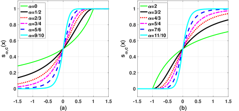
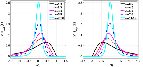
Figure 1: (a) SIGTRON $s_{\alpha,c}(x)$ with $\alpha=\frac{k-1}{k}<1$ ($k=1,2,3,4,6,10$) and $c_{\alpha}=-1$. Note that $s_{\alpha,c}(x)=1$, if $x\geq-c_{\alpha}$. (b) SIGTRON $s_{\alpha,c}(x)$ with $\alpha=\frac{k+1}{k}>1$ ($k=1,2,3,4,6,10$) and $c_{\alpha}=1$. Note that $s_{\alpha,c}(x)=0$, if $x\leq-c_{\alpha}$. (c) $\nabla s_{\alpha,c}(x)$ with $\alpha=\frac{k-1}{k}<1$ ($k=2,3,4,6,10$) and $c_{\alpha}=-1$. Note that $\nabla s_{\alpha,c}(x)=0$, if $x\geq-c_{\alpha}$. The inflection point $x_{ip}$ is getting close to $-c_{\alpha}=1$ as $\alpha\rightarrow 0$. (d) $\nabla s_{\alpha,c}(x)$ with $\alpha=\frac{k+1}{k}>1$ ($k=2,3,4,6,10$) and $c_{\alpha}=1$. Note that $\nabla s_{\alpha,c}(x)=0$, if $x\leq-c_{\alpha}$. The inflection point $x_{ip}$ is getting close to $-c_{\alpha}=-1$ as $\alpha\rightarrow 2$.

II SIGTRON: extended asymmetric sigmoid with Perceptron 

In this Section, we define SIGTRON using the extended exponential function $\exp_{\alpha,c}$ (7). We then study various properties of SIGTRON, such as its smoothness, inflection point, probability-half point, and parameterized mirror symmetry of the inflection point with respect to the probability-half point.

Definition II.1 (SIGTRON).

Let $\alpha\geq 0$, $c>0$, and $x\in{\mathbb{R}}$. Then SIGTRON(extended asymmetric sigmoid with Perceptron) is defined as

$$s_{\alpha,c}(x)=\left\{\begin{array}[]{l}\sigma_{\alpha,c}(x)\qquad\hbox{ if }x\in\hbox{dom}(\sigma_{\alpha,c})\\ \sigma_{P}(x)\qquad\;\;\hbox{ otherwise, }\end{array}\right.$$ (11)

where $\sigma_{\alpha,c}$ is the extended asymmetric sigmoid function

$$\sigma_{\alpha,c}(x)=\frac{c}{c+\exp_{\alpha,c}(-x)}.$$ (12)

Here, $\exp_{\alpha,c}$ is the extended exponential function (7) and $\sigma_{P}$ is the Perceptron function(or Heaviside function): $\sigma_{P}(x)=1$, if $x\geq 0$ and $0$, otherwise. The restricted domains of $\exp_{\alpha,c}$ and $\sigma_{\alpha,c}$ are defined in Table I. Note that $s_{\alpha,c}(x)\in[0,1]$ is a non-decreasing continuous function defined on ${\mathbb{R}}$ with $\lim_{x\rightarrow-\infty}s_{\alpha,c}(x)=0$ and $\lim_{x\rightarrow+\infty}s_{\alpha,c}(x)=1$. Additionally, $s_{\alpha,c}(0)=1/2$, irrespective of $\alpha$ and $c_{\alpha}$. Here $x_{ph}=0$ is denoted as the probability-half point. When $\alpha=1$, $s_{\alpha,c}(x)=\frac{1}{1+\exp(-x)}$ is the canonical sigmoid function, irrespective of $c$.

Note that SIGTRON with $c=1$ becomes the canonical sigmoid function as ${\left|\,\alpha-1\,\right|}\rightarrow 0$, since the extended exponential function with $c=1$ is the generalized exponential function. However, SIGTRON with ${\left|\,c_{\alpha}\,\right|}=1$ becomes a smoothed Perceptron as ${\left|\,\alpha-1\,\right|}\rightarrow 0$ and $\alpha\not=1$. Refer to Figure 1 for additional information.

In the following Theorem II.2, we characterize the smoothness of SIGTRON (11) depending on $\alpha$. The proof of Theorem II.2 is given in Appendix -A.

Theorem II.2.

For $n=1,2,3,\cdots$, when $\alpha\in\left(1-\frac{1}{n},1+\frac{1}{n}\right)$, the $n$-th derivative of $s_{\alpha,c}$ is continuous on ${\mathbb{R}}$ and expressed as

$$\nabla^{n}s_{\alpha,c}(x)=\left\{\begin{array}[]{l}\sum_{k=1}^{n}F_{n,k}(x)\quad\hbox{ if }x\in\hbox{dom}(\sigma_{\alpha,c})\\ \;0\qquad\quad\qquad\quad\;\hbox{ otherwise,}\end{array}\right.$$ (13)

where

$$F_{n,k}(x)=A_{n,k}\left(\frac{1}{1-\alpha}\right)\frac{c\exp^{k-n(1-\alpha)}_{\alpha,c}(-x)}{(c+\exp_{\alpha,c}(-x))^{k+1}},$$ (14)

and

$$A_{n,k}\left(\frac{1}{1-\alpha}\right)=(-1)^{n+k}k!\sum_{l=0}^{n}{\left[n\atop l\right]}{\left\{l\atop k\right\}}(\alpha-1)^{n-l}.$$ (15)

Here, $\left[n\atop l\right]$ is the Stirling number of the first kind  [42] with the recurrence equation $\left[n\atop l\right]=(n-1)\left[n-1\atop l\right]+\left[n-1\atop l-1\right]$, where $n,l\geq 1$. $\left\{l\atop k\right\}$ is the Stirling number of the second kind with the recurrence equation $\left\{l\atop k\right\}=k\left\{l-1\atop k\right\}+\left\{l-1\atop k-1\right\}$, where $l,k\geq 1$.

For the computation of the Stirling number of the first kind and the second kind, we need additional notational conventions: $\left\{0\atop 0\right\}=\left[0\atop 0\right]=1$ and $\left\{a\atop 0\right\}=\left[a\atop 0\right]=0$ for $a\geq 1$. We have $\left\{a\atop 1\right\}=1$ and $\left[a\atop 1\right]=(a-1)!$ with $0!=1$, for $a\geq 1$. Additionally, we note that $\left\{a\atop b\right\}=\left[a\atop b\right]=0$ if $b>a\geq 0$. For more details, refer to [42].

Theorem II.2 states that for any $\alpha\in(0,2)$, the gradient of $s_{\alpha,c}(x)$ is given by $c^{\alpha-1}(1-s_{\alpha,c}(x))^{\alpha}(s_{\alpha,c}(x))^{2-\alpha}$, where $x\in{\mathbb{R}}$. Check Figure 1 (c) and (d) for a visual representation of $\nabla s_{\alpha,c}(x)$. The information regarding the inflection point of $s_{\alpha,c}$ is provided in Corollary II.3. Additionally, we have observed that the function $\nabla s_{\alpha,c}(x)$ takes the form of the beta distribution $\beta_{D}(x;\alpha)=\frac{6}{\Gamma(3-\alpha)\Gamma(1+\alpha)}x^{2-\alpha}(1-x)^{\alpha}$, where $x\in[0,1]$. The cumulant distribution of the beta distribution, which has an adjustable parameter $\alpha$, can also be classified as an S-shaped sigmoid function.

Corollary II.3.

For $\alpha\in(0,2)$, the inflection point $x_{ip}$ of SIGTRON $s_{\alpha,c}$ exists in the interval $int(\hbox{dom}(\sigma_{\alpha,c}))$ and is expressed as

$$x_{ip}=-\ln_{\alpha,c}\left(\frac{c\alpha}{2-\alpha}\right).$$

When $\alpha=1$, the inflection point is the probability-half point, that is, $x_{ip}=x_{hp}=0$.

Proof.

From (13) and Appendix -A, we know that $s_{\alpha,c}\in C^{\infty}(int(\hbox{dom}(\sigma_{\alpha,c})))$ and $\nabla^{2}s_{\alpha,c}(x)=\frac{-\alpha c\exp_{\alpha,c}^{2\alpha-1}(-x)}{(c+\exp_{\alpha,c}(-x))^{2}}+\frac{2c\exp_{\alpha,c}^{2\alpha}(-x)}{(c+\exp_{\alpha,c}(-x))^{3}}.$ Let $\alpha\not=1$, then, since $\exp_{\alpha,c}(-x)\not=0$ for $x\in int(\hbox{dom}(\sigma_{\alpha,c}))$, the inflection point $x_{ip}$ is a point satisfying $x_{ip}=-\ln_{\alpha,c}\left(\frac{c\alpha}{2-\alpha}\right).$ If $\alpha=1$, then $s_{\alpha,c}$ is the canonical sigmoid function. Thus, $x_{ip}=x_{hp}=0$.       

Figure 1 shows $s_{\alpha,c}$ and its derivative for various choices of $\alpha$ satisfying ${\left|\,\alpha-1\,\right|}=\frac{1}{k}$ ($k=1,2,3,4,6,10$) and ${\left|\,c_{\alpha}\,\right|}=1$. Note that $\nabla s_{\alpha,c}$ is not defined at $\alpha=0$ and $\alpha=2$. When $\alpha>1$, the inflection point $x_{ip}$ is getting close to $-1$ as $\alpha\rightarrow 2$. On the other hand, when $\alpha<1$, the inflection point $x_{ip}$ is getting close to $1$ as $\alpha\rightarrow 0$.

Remark II.4.

SIGTRON is a general framework for replacing the S-shaped sigmoid function in diverse machine learning problems requiring adjustability of probability(or inflection point) and fixed probability-half point. For instance, refer to the simplified first-order optimal equation for classification (9) and Example II.5. As canonical sigmoid function $\sigma(x)=\frac{1}{1+\exp(-x)}$ has a symmetric property $\sigma(x)=1-\sigma(-x)$, SIGTRON $s_{\alpha,c}$ also has an extended symmetric property:

$$s_{\alpha,c}(x)=1-s_{2-\alpha,c^{-1}}(-x)$$ (16)

where $\alpha\in[0,2]$. Also, for $\alpha\in(0,2)$, we have $\nabla s_{\alpha,c}(x)=\nabla s_{2-\alpha,c^{-1}}(-x)$, the parameterized mirror symmetry with respect to probability-half point $x_{hp}=0$. See Figure 1 (c) and (d) for examples of parameterized mirror symmetry of $\nabla s_{\alpha,c}$. It is worth commenting that the gradient of Logitron $L_{\alpha,c}$ [15] is also a negative probability function, of which the probability-half point depends on $\alpha$. For $\alpha\in(0,2]$, we have

$$\nabla L_{\alpha,c}(x)=-(s_{2-\alpha,c^{-1}}(-x))^{\alpha}$$ (17)

where the exponent $\alpha$ is an acceleration parameter of SIGTRON $s_{2-\alpha,c^{-1}}(-x)$ and (16) is used.

Example II.5.

It is well-known that it is hard to give a probability for the results of max-margin SVM classifier [43, 44]. In fact, [44] uses the canonical sigmoid function $\sigma(\gamma x+\xi)$ to fit a probability to the classified results of the SVM. Here $\gamma$ and $\xi$ should be estimated [41]. Instead of fitting with the canonical sigmoid function $\sigma(\gamma x+\xi)$, we could use SIGTRON $s_{\alpha,c}$ as a probability estimator for the results of the SVM classifier or any other classifiers having decision boundary, such as hyperplane. For this purpose, there are three steps to follow. First, we must place the probability-half point $x_{hp}$ of $s_{\alpha,c}$ at the decision boundary. Second, we should adjust $c_{\alpha}$ to place the exact probability-one point of $s_{\alpha,c}$ at a specific point, such as the maximum margin point. Finally, we only need to estimate $\alpha$ for the decreasing slope of $s_{\alpha,c}$ based on the distribution of classified results. See [45] for the probability estimation issues in deep neural networks.

III Virtual SIGTRON-induced loss function, SIC(SIGTRON-imbalanced classification) model, and skewed hyperplane equation

This Section studies the SIC model with the virtual SIGTRON-induced loss functions and the skewed hyperplane equation of the SIC model.

Definition III.1.

Let $\alpha\in[0,2]$, $c>0$, and $x\in{\mathbb{R}}$, then the virtual SIGTRON-induced loss function $L_{\alpha,c}^{S}$ is defined by the following gradient equation

$$\nabla L^{S}_{\alpha,c}(x)=s_{\alpha,c}(x)-1,$$ (18)

where $s_{\alpha,c}(x)-1$ is a negative probability function. By the extended symmetric property of SIGTRON in (16), we have $s_{\alpha,c}(x)-1=-s_{2-\alpha,c^{-1}}(-x)$.

We notice that an expansion of the class of Logitron loss (17) via virtualization is easily achieved by $\nabla{L}_{\beta,\alpha,c}(x)=-(s_{2-\alpha,c^{-1}}(-x))^{\beta}$ where $\beta>0$ is a tuning parameter which controls the location of probability-half point $x_{hp}$. Thus, the virtualized Logitron loss contains both the virtual SIGTRON-induced loss (18) and the Logitron loss (17).

Lemma III.2.

Let $\alpha\in[0,1)\cup(1,2]$ and $c>0$. Then the virtual SIGTRON-induced loss function $L^{S}_{\alpha,c}$ satisfying (18) has the following integral formulations:
(1) Case $\alpha\in(1,2]$:

$$L_{\alpha,c}^{S}(x)=\left\{\begin{array}[]{l}-c_{\alpha}F\left(1+\frac{x}{c_{\alpha}};\alpha-1\right)+c_{\alpha}\;\;\hbox{ if }x\geq-c_{\alpha}\\ -x\hskip 115.63243pt\hbox{ otherwise. }\end{array}\right.$$ (19)

(2) Case $\alpha\in[0,1)$:

$$L_{\alpha,c}^{S}(x)=\left\{\begin{array}[]{l}c_{\alpha}F\left(1+\frac{x}{c_{\alpha}};1-\alpha\right)-c_{\alpha}-x\;\;\hbox{ if }x\leq-c_{\alpha}\\ 0\hskip 137.31255pt\hbox{ otherwise. }\end{array}\right.$$ (20)

Here, $F(z;b)=\int_{0}^{z}\frac{1}{1+t^{1/b}}dt$ with $z\in{\mathbb{R}}_{\geq 0}$ and $b>0$.

Proof.

(1) Case $\alpha\in(1,2]$: From (18), we have

$$\nabla L_{\alpha,c}^{S}(x)=\left\{\begin{array}[]{l}-\frac{1}{1+(1+\frac{x}{c_{\alpha}})^{\frac{1}{\alpha-1}}}\;\;\;\;\;\hbox{ if }x\geq-c_{\alpha}\\ -1\qquad\qquad\qquad\;\;\hbox{ otherwise, }\end{array}\right.$$

where $-c_{\alpha}<0$ and $1+\frac{x}{c_{\alpha}}\geq 0$. The integration of $\nabla L^{S}_{\alpha,c}$ becomes

$$L^{S}_{\alpha,c}(a_{1})-L^{S}_{\alpha,c}(a_{0})=\int_{a_{0}}^{a_{1}}\nabla L^{S}_{\alpha,c}(t)dt=\left\{\begin{array}[]{l}-c_{\alpha}F(1+a_{1}/c_{\alpha};\alpha-1)+c_{\alpha}+a_{0},\;\hbox{ if }a_{1}\geq-c_{\alpha}\\ -a_{1}+a_{0},\hskip 120.69077pt\hbox{ otherwise, }\end{array}\right.$$

where we may choose $a_{0}\ll-c_{\alpha}$. Then, we get the virtual SIGTRON-induced loss function (19), after setting $a_{1}=x$ and removing constants.

(2) Case $\alpha\in[0,1)$: We have

$$\nabla L_{\alpha,c}^{S}(x)=\left\{\begin{array}[]{l}\frac{1}{1+(1+\frac{x}{c_{\alpha}})^{\frac{1}{1-\alpha}}}-1\quad\quad\hbox{ if }x\leq-c_{\alpha}\\ 0\hskip 90.3375pt\hbox{ otherwise, }\end{array}\right.$$

where $-c_{\alpha}>0$ and $1+\frac{x}{c_{\alpha}}\geq 0$. Thus, we get

$$L^{S}_{\alpha,c}(a_{0})-L^{S}_{\alpha,c}(a_{1})=\int_{a_{1}}^{a_{0}}\nabla L^{S}_{\alpha,c}(t)dt=\left\{\begin{array}[]{l}-c_{\alpha}F(1+\frac{a_{1}}{c_{\alpha}};1-\alpha)+c_{\alpha}+a_{1}\quad\hbox{ if }a_{1}\leq-c_{\alpha}\\ 0\hskip 151.76744pt\hbox{ otherwise, }\end{array}\right.$$

where $a_{0}>-c_{\alpha}$. Let $a_{1}=x$, then we get the virtual SIGTRON-induced loss function (20).       

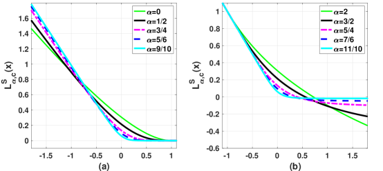
Figure 2: Graphs of the virtual SIGTRON-induced loss function $L^{S}_{\alpha,c}$ for (a) $\alpha=\frac{k-1}{k}$ with $c_{\alpha}=-1$ and (b) $\alpha=\frac{k+1}{k}$ with $c_{\alpha}=1$. Here $k=1,2,4,6$, and $10$. In the case of $k=1,2,4,6$, $L_{\alpha,c}^{S}$ has a closed-form expression. See Example III.3.

In Figure 2, we present the virtual SIGTRON-induced loss $L_{\alpha,c}^{S}(x)$ with ${\left|\,c_{\alpha}\,\right|}=1$ and ${\left|\,\alpha-1\,\right|}=\frac{1}{k}$. Here $k=1,2,4,6$ and $10$ are the polynomial orders of $\exp_{\alpha,c}$. For $k=10$, $L_{\alpha,c}^{S}(x)$ is computed directly by (19) and (20). For $k=1,2,4,6$, $L_{\alpha,c}^{S}(x)$ is expressed in a closed form by virtue of Example III.3. As we increase the polynomial order $k=\frac{1}{{\left|\,\alpha-1\,\right|}}$, i.e. $\alpha\rightarrow 1$ and ${\left|\,c_{\alpha}\,\right|}=1$, $L_{\alpha,c}^{S}(x)$ is getting close to the smoothed Perceptron loss function [46], not to the logistic loss.

Example III.3.

We make a list of $F(a;1/k)$ for $k=1,\cdots,6$.

• $k=1:$ $F(a;1/1)=\ln(1+a)$

• $k=2:$ $F(a;1/2)=\arctan(a)$

• $k=3:$ $F(a;1/3)=\frac{1}{6}\log\left(1+\frac{3a}{a^{2}-a+1}\right)+\frac{1}{\sqrt{3}}\arctan\left(\frac{2a-1}{\sqrt{3}}\right)-\frac{1}{\sqrt{3}}\arctan\left(-\frac{1}{\sqrt{3}}\right)$

• $k=4:$ $F(a;1/4)=\frac{1}{4\sqrt{2}}\log\left(1+\frac{2\sqrt{2}a}{a^{2}-\sqrt{2}a+1}\right)+\frac{1}{2\sqrt{2}}\arctan\left(1+\sqrt{2}a\right)-2\arctan(1-\sqrt{2}a)$

• $k=5:$ $F(a;1/5)=\frac{(\sqrt{5}-1)}{20}\log(2a^{2}+(\sqrt{5}-1)a+2)-\frac{(\sqrt{5}+1)}{20}\log(2a^{2}-(\sqrt{5}+1)a+2)+\frac{\log(1+a)}{5}\\ ~{}~{}~{}~{}~{}~{}~{}~{}~{}~{}~{}~{}~{}~{}~{}~{}~{}~{}~{}~{}~{}~{}~{}~{}~{}~{}~{}~{}-\frac{\sqrt{10-2\sqrt{5}}}{10}\arctan\left(\frac{-4a+\sqrt{5}+1}{\sqrt{10-2\sqrt{5}}}\right)+\frac{\sqrt{10+2\sqrt{5}}}{10}\arctan\left(\frac{4a+\sqrt{5}-1}{\sqrt{10+2\sqrt{5}}}\right)-\frac{(\sqrt{5}-1)\log 2+(\sqrt{5}+1)\log 2}{20}\\ ~{}~{}~{}~{}~{}~{}~{}~{}~{}~{}~{}~{}~{}~{}~{}~{}~{}~{}~{}~{}~{}~{}~{}+\frac{\sqrt{10-2\sqrt{5}}}{10}\arctan\left(\frac{\sqrt{5}+1}{\sqrt{10-2\sqrt{5}}}\right)-\frac{\sqrt{10+2\sqrt{5}}}{10}\arctan\left(\frac{\sqrt{5}-1}{\sqrt{10+2\sqrt{5}}}\right)$

• $k=6:$ $F(a;1/6)=\sqrt{3}\log\left(\frac{a^{2}+\sqrt{3}a+1}{a^{2}-\sqrt{3}a+1}\right)+\arctan(\sqrt{3}+2a)/6-\arctan(\sqrt{3}-2a)/6+\arctan(a)/3$

III-A Learning a hyperplane with SIC model

Let us first consider the cost-sensitive convex minimization model (8) to find a hyperplane $h^{*}(x)=0$ from the given training dataset ${\cal D}$. The following is the reformulation of (8) through the virtual SIGTRON-induced loss function (18) and $\ell_{2}$-regularizer.

$$h^{*}=\mathop{\rm arg\,min}_{h\in{\cal H}}\;{\cal F}(h)$$ (24)

where ${\cal H}=\{\left\langle w,\,\cdot\right\rangle+b\;|\;(w,b)\in{\mathbb{R}}^{s}\times{\mathbb{R}}\}$ and

$${\cal F}(h)=\sum_{i\in{\cal N}_{+}}L^{S}_{\alpha_{+},c_{+}}(h(x_{i}))+\sum_{j\in{\cal N}_{-}}L^{S}_{\alpha_{-},c_{-}}(-h(x_{j}))+\frac{\lambda}{2}\|w\|_{2}^{2}.$$ (25)

This minimization problem (24) with (25) is named as the SIGTRON-imbalanced classification(SIC) model. To demonstrate the merit of SIC model (24), we start with the following simplified first-order optimal equation for classification introduced in (9) with $p_{+}(x)=s_{2-\alpha_{+},c_{+}^{-1}}(-x)$ and $p_{-}(x)=s_{2-\alpha_{-},c_{-}^{-1}}(-x)$.

$$\boxed{r_{sc}s_{2-\alpha_{+},c_{+}^{-1}}(-h^{*}(x_{p}^{c}))=s_{2-\alpha_{-},c_{-}^{-1}}(h^{*}(x_{n}^{c}))}$$ (26)

where $x_{p}^{c}$ is the centroid of the positive training dataset $x_{i}\in{\cal N}_{+}$ and $x_{n}^{c}$ is the centroid of the negative training dataset $x_{j}\in{\cal N}_{-}$. In the following Theorem III.4, the skewed hyperplane equation of the SIC model (24) is derived from a first-order approximation to (26).

Theorem III.4.

Let $\|x_{p}^{c}-x_{n}^{c}\|>a$ for a positive constant $a$, $h^{*}(x_{p}^{c})\in dom(\sigma_{\alpha_{+},c_{+}})$, $0<h^{*}(x_{p}^{c})\ll{\left|\,c_{\alpha_{+}}\,\right|}$, $-h^{*}(x_{n}^{c})\in dom(\sigma_{\alpha_{-},c_{-}})$, and $0<-h^{*}(x_{n}^{c})\ll{\left|\,c_{\alpha_{-}}\,\right|}$. Here, $c_{\alpha_{+}}=c_{+}^{1-\alpha_{+}}/(\alpha_{+}-1)$, $c_{\alpha_{-}}=c_{-}^{1-\alpha_{-}}/(\alpha_{-}-1)$, and $\alpha_{+},\alpha_{-}\in[0,1)\cup(1,2]$. Then, from (26), we have the skewed hyperplane equation

$$\left\langle w^{*},\,\left(\frac{c_{+}^{\alpha_{+}-1}x_{p}^{c}+r_{sc}c_{-}^{\alpha_{-}-1}x_{n}^{c}}{c_{+}^{\alpha_{+}-1}+r_{sc}c_{-}^{\alpha_{-}-1}}\right)\right\rangle+b^{*}\approx\frac{2(r_{sc}-1)}{c_{+}^{\alpha_{+}-1}+r_{sc}c_{-}^{\alpha_{-}-1}},$$ (27)

where $r_{sc}$ is the scale-class-imbalance ratio (1). If $r_{sc}=1$, then the signed distance of $x_{p}^{c}$ to the hyperplane $h^{*}(x)=0$ is approximately given as

$$\frac{h^{*}(x_{p}^{c})}{\|w^{*}\|}\approx\eta\|x_{p}^{c}-x_{n}^{c}\|cos(\theta_{+})$$ (28)

where $\eta=\frac{c_{-}^{\alpha_{-}-1}}{c_{+}^{\alpha_{+}-1}+c_{-}^{\alpha_{-}-1}}\in(0,1)$ and $cos(\theta_{+})=\left\langle\frac{w^{*}}{\|w^{*}\|},\,\frac{x_{p}^{c}-x_{n}^{c}}{\|x_{p}^{c}-x_{n}^{c}\|}\right\rangle>0$. In the same way, for $x_{n}^{c}$, we have $\frac{h^{*}(x_{n}^{c})}{\|w^{*}\|}\approx(\eta-1)\|x_{p}^{c}-x_{n}^{c}\|cos(\theta_{+})$.

Proof.

We get $r_{sc}\left(1+\left(1-\frac{h^{*}(x_{n}^{c})}{c_{\alpha_{-}}}\right)^{\frac{1}{\alpha_{-}-1}}\right)=\left(1+\left(1+\frac{h^{*}(x_{p}^{c})}{c_{\alpha_{+}}}\right)^{\frac{1}{\alpha_{+}-1}}\right)$ from (26). Since $0<{\left|\,\frac{h^{*}(x_{p}^{c})}{c_{\alpha_{+}}}\,\right|}\ll 1$ and $0<{\left|\,\frac{h^{*}(x_{n}^{c})}{c_{\alpha_{-}}}\,\right|}\ll 1$, we have the first order approximation

$$r_{sc}\left(2-\frac{h^{*}(x_{n}^{c})}{c_{-}^{1-\alpha_{-}}}\right)\approx\left(2+\frac{h^{*}(x_{p}^{c})}{c_{+}^{1-{\alpha_{+}}}}\right),$$ (29)

where $(\alpha_{-}-1)c_{\alpha_{-}}=c_{-}^{1-\alpha_{-}}$ and $(\alpha_{+}-1)c_{\alpha_{+}}=c_{+}^{1-\alpha_{+}}$. Note that, when $0\leq\alpha<1$ and ${\left|\,r\,\right|}\ll 1$, we use $(1+r)^{\frac{1}{\alpha-1}}\approx(1-r)^{\frac{1}{1-\alpha}}\approx 1+\frac{1}{\alpha-1}r$. By simplifying (29), we get the skewed hyperplane equation in (27). If $r_{sc}=1$ then $-b^{*}\approx\left\langle w^{*},\,\eta x_{p}^{c}+(1-\eta)x_{n}^{c}\right\rangle$ with $\eta=\frac{c_{-}^{\alpha_{-}-1}}{c_{+}^{\alpha_{+}-1}+c_{-}^{\alpha_{-}-1}}$. Thus, the signed distance of $x_{p}^{c}$ to the hyperplane $h^{*}(x)=0$ in (28) is easily derived.       

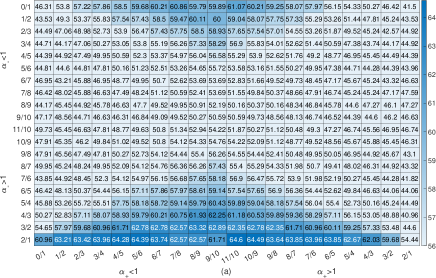
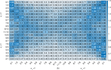
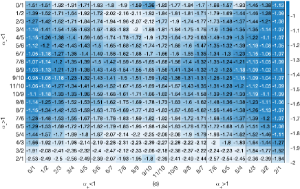
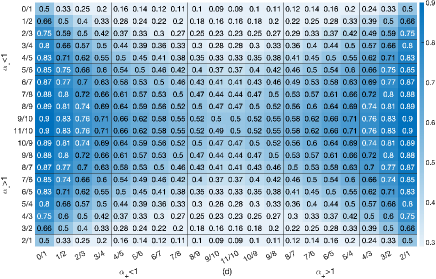
Figure 3: Classification results with the spectf dataset in Table V. The test dataset has $r_{sc}=0.26(r_{c}=0.09)$. However, the training dataset is well-balanced, i.e., $r_{sc}=1$. We have $20\times 20$ hyperplanes $h^{*}_{(\alpha_{+},\alpha_{-})}(x)=0$ by solving $20\times 20$ SIC models (24) with the well-balanced training dataset. (a) The pattern of the test classification accuracy. (b) The pattern of the signed distance of the centroid of the positive test dataset to the hyperplane. (c) The pattern of the signed distance of the centroid of the negative test dataset to the hyperplane. (d) The pattern of $\eta$ in (30). The best test accuracy is achieved at $(\alpha_{+},\alpha_{-})=(\frac{11}{10},2)$. This point is the smallest distance of the centroid of the positive test dataset to the hyperplane. And, it is contained in the group $\left\{(\frac{11}{10},2),(\frac{9}{10},2),(\frac{11}{10},0),(\frac{9}{10},0)\right\}$ having the smallest $\eta=\frac{1}{11}$. See Example III.5 for more details.

In practice, due to computational constraints, we normally choose polynomial functions for $\exp_{\alpha,c}$, i.e., positive integers for $\frac{1}{{\left|\,\alpha_{\pm}-1\,\right|}}$. Assume that ${\left|\,c_{\alpha_{\pm}}\,\right|}$ is a constant, $\frac{1}{{\left|\,\alpha_{+}-1\,\right|}}=k_{+}$, and $\frac{1}{{\left|\,\alpha_{-}-1\,\right|}}=k_{-}$. Here, $k_{\pm}=1,2,3,\cdots$. Then we have

$$\eta=\frac{1/c_{-}^{1-\alpha_{-}}}{1/c_{+}^{1-\alpha_{+}}+1/c_{-}^{1-\alpha_{-}}}=\frac{k_{-}}{k_{+}+k_{-}}$$ (30)

The hyperplane $h^{*}(x)=0$ is tuned by the ratio of polynomial order of SIGTRON if $\cos(\theta_{+})$ does not change much. The following Example III.5 describes the tunable hyperplane through $r_{sc}$-inconsistent dataset having a well-balanced training dataset.

Example III.5.

Let us start with the two-class ‘ spectf ’ dataset in Table V. The training dataset is well-balanced, i.e., $r_{sc}=1$. However, the test dataset has $r_{sc}=0.26$($r_{c}=0.09$). It indicates that the positive class of the test dataset is the minority class. The hyperplane to be learned should be located near the minority class to achieve better test classification accuracy. As observed in (28) and Figure 3 (d), to move the hyperplane to the minority class as close as we can, we need to select the smallest $\eta=1/11$. This $\eta$ corresponds to four $(\alpha_{+},\alpha_{-})$ candidates: $(11/10,2)$,$(9/10,2)$,$(11/10,0)$, and $(9/10,0)$. In fact, at $(\alpha_{+},\alpha_{-})=(11/10,2)$, we obtain the minimum distance of $x_{test,p}^{c}$ (the centroid of the positive class of test dataset) to the hyperplane $h_{(\alpha_{+}=11/10,\alpha_{-}=2)}^{*}(x)=0$ (Figure 3 (b)) and the best test classification accuracy $64.6\%$ (Figure 3 (a)). Note that the pattern of $\eta$ in Figure 3 (d) is similar to the pattern of the distance of $x_{test,p}^{c}$ to the hyperplane in Figure 3 (b). As Figure 3 (a) shows, the region $\alpha_{-}\approx 2$ obtains better test classification accuracy than the region $\alpha_{-}\approx 0$. Additionally, note that $cos(\theta_{test,+})=\left\langle\frac{w_{(\alpha_{+},\alpha_{-})}^{*}}{\|w_{(\alpha_{+},\alpha_{-})}^{*}\|},\,\frac{x_{test,p}^{c}-x_{test,n}^{c}}{\|x_{test,p}^{c}-x_{test,n}^{c}\|}\right\rangle\in[0.52,0.90]$ and ${\bf E}(cos(\theta_{test,+}))=0.71$. As a reference, we obtained $20\times 20$ hyperplanes $h^{*}_{(\alpha_{+},\alpha_{-})}(x)=0$ by solving $20\times 20$ SIC models (24) with the well-balanced training dataset. The cross-validation was used for the best regularization parameter $\lambda$. We set ${\left|\,c_{\alpha_{\pm}}\,\right|}=2$, $\frac{1}{{\left|\,1-\alpha_{+}\,\right|}}=k_{+}=1,2,\cdots,10$, and $\frac{1}{{\left|\,1-\alpha_{-}\,\right|}}=k_{-}=1,2,\cdots,10$.

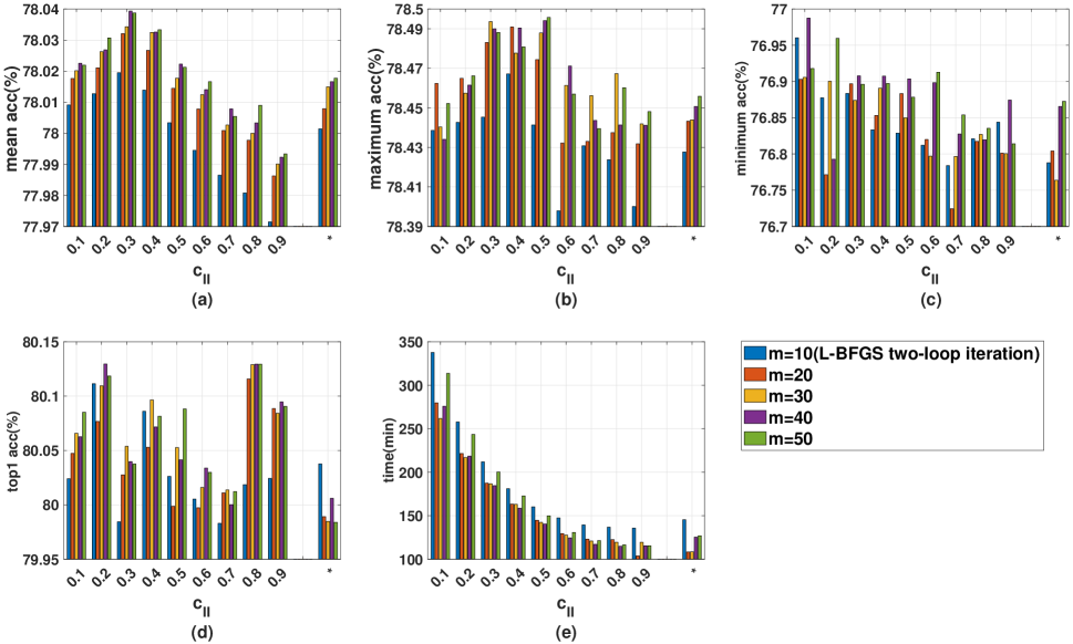
Figure 4: A comparison of performanve between quasi-Newton(L-BFGS) for virtual convex loss, which uses the strong Wolfe condition (36) with $c_{II}\in[0.1,0.9]$, and the classic L-BFGS(*), which uses the strong Wolfe condition (36) with $c_{II}=0.9$ and the Armijo condition (31) with $c_{I}=10^{-4}$. Note that L-BFGS(*) uses the cubic-interpolation-based line search [27, 28]. For our experiments, we use $12\times 12$ SIC models with ${\left|\,c_{\alpha}\,\right|}=1$ and ${\left|\,\alpha_{\pm}-1\,\right|}=\frac{1}{k}$, where $k=1,2,3,4,5,6$. (a) Mean test accuracy of $12\times 12$ SIC models. (b) Maximum test accuracy and (c) minimum test accuracy obtained by an SIC model with fixed $\alpha_{\pm}$ for each $c_{II}$. (d) Test accuracy of TOP$1$ for each $c_{II}$. (e) Total computation time of $12\times 12$ SIC models. Here, we report the average values of five times repeated experiments with all datasets in Table V and VI. For $0.1\leq c_{II}\leq 0.5$, in terms of mean test classification accuracy in (a), quasi-Newton(L-BFGS) for virtual convex loss outperforms L-BFGS(*), for each $m$ of two loop iterations.

Remark III.6.

Lately, [9] has proposed two focal loss functions for imbalanced object detection. The first one is the non-convex focal loss function. It has $L_{+}(h(x))=-\pi(1-p(h(x)))^{\gamma_{g}}\log(p(h(x)))$ and $L_{-}(h(x))=-(1-\pi)p(h(x))^{\gamma_{g}}\log(1-p(h(x)))$ where $p(h(x))\in(0,1)$ is a probability function, like canonical sigmoid $\sigma$ or reduced Sigtron. The second one is the convex focal loss function. It has $L_{+}(h(x))=-\pi\log(\sigma(\gamma h(x)+\xi))$ and $L_{-}(h(x))=-(1-\pi)\log(1-\sigma(\gamma h(x)+\xi))$. Here $\pi\in(0,1)$ is known as a cost-sensitive parameter to be selected depending on $r_{sc}$ of the training dataset. Note that $\gamma\geq 1$ and $\xi\geq 0$ control the stiffness and shift of the convex focal loss, respectively. As [9] mentioned, the performance gap between the two types of focal losses is negligible. Therefore, we exclusively compare the convex focal loss to the SIC model. Unlike the latter, which uses an external $\pi$-weight, the SIC model employs a virtualized convex loss function with internal polynomial parameters. To find additional information, please refer to Section V-A.

IV Quasi-Newton optimization(L-BFGS) for virtual convex loss

This Section presents quasi-Newton optimization(L-BFGS) for virtual convex loss framework. It includes the proposed interval-based bisection line search, which uses gradients of a virtual convex loss function.

Let us discuss the SIC model (24), where ${\cal F}(h)$ is convex, differentiable, and bounded below. It is worth noting that the optimization framework we will be proposing for this model can also be used for cost-sensitive learning model (8), including the $\pi$-weighted convex focal loss. Before we proceed, let us take a moment to review the quasi-Newton optimization framework described in [27]. The iterates $h_{0},h_{1},h_{2},\cdots$ satisfy $h_{t+1}=h_{t}+\rho_{t}z_{t}$ where $\rho_{t}>0$ is a step length and $z_{t}=-B_{t}^{-1}\nabla{\cal F}(h_{t})$ is a descent direction. Here, $B_{t}$ is a symmetric and positive definite rank-two approximation of the Hessian matrix $\nabla^{2}{\cal F}(h_{t})$. Interestingly, L-BFGS directly approximates $B_{t}^{-1}\nabla{\cal F}(h_{t})$ by two-loop iterations with $m$ recent elements. Here, $m$ is the tuning parameter of L-BFGS. The performance comparison of the proposed optimization framework considering $m$ of L-BFGS is shown in Figure 4. For the initial point, we set $h_{0}=0$, corresponding to the probability-half point of SIGTRON in the gradient of the SIC model. It is well known that, to guarantee sufficient descent of ${\cal F}(h)$ and positive definiteness of low-rank matrix $B_{t}$, the step length $\rho_{t}$ of L-BFGS should satisfy the Armijo condition (31) and the Wolfe condition (32):

$${\cal F}(h_{t}+\rho_{t}z_{t})-{\cal F}(h_{t})\leq c_{I}\rho_{t}\left\langle\nabla{\cal F}(h_{t}),\,z_{t}\right\rangle$$ (31)

and

$$\left\langle\nabla{\cal F}(h_{t}+\rho_{t}z_{t}),\,z_{t}\right\rangle\geq c_{II}\left\langle\nabla{\cal F}(h_{t}),\,z_{t}\right\rangle,$$ (32)

where $0<c_{I}<c_{II}<1$. The Armijo condition (31) can be reformulated through the expectation of gradients:

$$\phi(\rho_{t})-\phi(0)=\int_{0}^{\rho_{t}}\phi^{\prime}(\rho)d\rho=\rho_{t}{\bf E}_{[0,\rho_{t}]}(\phi^{\prime}),$$ (33)

where $\phi(\rho_{t})={\cal F}(h_{t}+\rho_{t}z_{t})$ and $\phi^{\prime}(\rho)=\left\langle\nabla{\cal F}(h_{t}+\rho z_{t}),\,z_{t}\right\rangle$. Note that $\phi^{\prime}(0)=\left\langle\nabla{\cal F}(h_{t}),\,z_{t}\right\rangle<0$ where $z_{t}=-B_{t}^{-1}\nabla{\cal F}(h_{t})$. Now, we get the reformulated Armijo condition

$${\bf E}_{[0,\rho_{t}]}(\phi^{\prime})\leq c_{I}\phi^{\prime}(0)$$ (34)

and the Wolfe condition

$$c_{II}\phi^{\prime}(0)\leq\phi^{\prime}(\rho_{t}),$$ (35)

where (35) is also known as the curvature condition [47], which is clearly understood by the reformulation of (35) as ${\bf E}_{[0,\rho_{t}]}(\phi^{\prime\prime})>(c_{II}-1)\rho_{t}\phi^{\prime}(0)>0$. The positive definiteness of $B_{t}$ in L-BFGS is adjusted by $c_{II}\in(0,1)$, normally set as $0.9$. For more details, see [27].

The reformulated Armijo condition (34) has several advantages, compared to the Armijo condition (31). First, it is more intuitive about the descent condition of the loss function. The average slopes of $\phi$ in the interval $[0,\rho_{t}]$ must be less than the initial slope $\phi^{\prime}(0)$. Second, for the SIC model (24), using an approximation of (34) is more practical. That is, ${\bf E}_{[0,\rho_{t}]}(\phi^{\prime})\approx\sum_{i=1}^{n}a_{i}\phi^{\prime}(\tilde{\rho}_{i})$, where $a_{i}\geq 0$, $\sum_{i=1}^{n}a_{i}=1$, and $0\leq\tilde{\rho}_{0}<\tilde{\rho}_{1}<\cdots<\tilde{\rho}_{n}\leq\rho_{t}$. This approach is workable for the general loss function, including virtual non-convex loss function. For a virtual convex loss function, however, we do not need to evaluate a relatively large number of directional derivatives in the interval $[0,\rho_{t}]$. Instead of (34) and (35), we can use the strong Wolf condition, i.e., (relative) strong Wolfe stopping criterion.

$${\left|\,\phi^{\prime}(\rho_{t})\,\right|}\leq-c_{II}\phi^{\prime}(0)$$ (36)

where $c_{II}\in(0,1)$ is a tuning parameter of the proposed quasi-Newton(L-BFGS) optimization for virtual convex loss. See also [30, 31] for related line search algorithms utilizing (36). In this article, for the strong-Wolfe stopping criterion (36), we create a new interval-based bisection line search(Algorithm 2). See [27, 48] for the various characteristics of the interval reduction method in general line search. The overall framework of quasi-Newton(L-BFGS) optimization for virtual convex loss is stated in Algorithm 1, which contains the interval-based bisection line search in Algorithm 2. See also Theorem IV.1 for the convergence of Algorithm 2.

1 Input: $h_{0}=(w_{0},b_{0})=0$, $\epsilon_{tol1}=10^{-2}$, $\epsilon_{tol2}=10^{-4}$, $c_{II}=0.4$, $MaxIter=100$.

2 Output: $h^{*}=(w^{*},b^{*})$.

3 for  $0\leq r\leq MaxIter$ do

4       if $\|\nabla{\cal F}(h_{t})\|_{\infty}\leq\epsilon_{tol1}$ or $\|h_{t+1}-h_{t}\|_{\infty}\leq\epsilon_{tol2}$ then

5            $h^{*}=h_{t}$ and STOP

6      Compute descent direction $z_{t}$ by Quasi-Newton optimization(L-BFGS)

7      

$$z_{t}=\hbox{L-BFGS}(\nabla{\cal F}(h_{t}))$$

Compute step-Length $\rho_{t}$ by Algorithm 2 with strong-Wolfe stopping criterion (36)

8      

$$\rho_{r}=\mathop{\rm arg\,min}_{\rho\in{\mathbb{R}}_{\geq 0}}{\cal F}(h_{t}+\rho z_{t})$$

Update $h_{t+1}=h_{t}+\rho_{t}z_{t}$

$h^{*}=h_{MaxIter+1}$

Algorithm 1 Quasi-Newton optimization(L-BFGS) for virtual convex loss

Theorem IV.1.

Let $\phi$ be convex, differentiable, and bounded below. Then Algorithm 2 with an initial condition $\phi^{\prime}(0)<0$ converges to $\rho^{*}$ satisfying (36), where $c_{II}\in(0,1)$, in finite steps.

Proof.

Let us first consider the case that $\phi$ is a coercive function. Since $\phi^{\prime}(0)<0$ and $\phi^{\prime}$ is a non-decreasing function, there is $\rho_{opt}>0$ such that $\phi^{\prime}(\rho)\geq 0$ for all $\rho\geq\rho_{opt}$. As noticed in line $6-7$ and line $10-11$ of Algorithm 2, there is $i$th iteration such that $\phi^{\prime}(\rho_{i})<\phi^{\prime}(\rho_{opt})=0<\phi^{\prime}(2\rho_{i})$. Therefore, the interval, which includes $\rho_{opt}$, is established as $[\rho_{L},\rho_{U}]=[\rho_{i},2\rho_{i}]$. Then by the bisection algorithm in line $6-9$ and line $13$, $[\rho_{L},\rho_{U}]$ is shrinking to $\rho_{opt}$ and the strong-Wolfe stopping criterion in line $4$ of Algorithm 2 is satisfied within finite steps. Now, we consider the case that $\phi$ is not a coercive function. Since $\phi$ is convex, bounded below, and $\phi^{\prime}(0)<0$, $\lim_{\rho\rightarrow+\infty}\phi^{\prime}(\rho)\rightarrow 0$(line $11$). Therefore, it stops by strong-Wolfe stopping criterion in line $4$.       

1 Input: $c_{II}=0.4$, $itermax=100$, $\rho_{0}$, $\phi^{\prime}(\rho)=\left\langle\nabla{\cal F}(h_{t}+\rho z_{t}),\,z_{t}\right\rangle$, $\phi^{\prime}(0)<0$, $[\rho_{L},\rho_{U}]=[0,\infty]$

2 Output: $\rho^{*}$

3 for $0\leq i\leq$ itermax do

4       if  ${\left|\,\phi^{\prime}(\rho_{i})\,\right|}\leq-c_{II}\phi^{\prime}(0)$  then

5             $\rho^{*}=\rho_{i}$ and STOP

6            

7      if $0<\phi^{\prime}(\rho_{i})$ then

8             $\rho_{U}=\rho_{i}$  

9      else if $\phi^{\prime}(\rho_{i})<0$ then

10             $\rho_{L}=\rho_{i}$  

11      if $\rho_{U}=\infty$ then

12            

13            $\rho_{i+1}=2\rho_{L}$

14      else

15             $\rho_{i+1}=\frac{1}{2}(\rho_{L}+\rho_{U})$

16      

17$\rho^{*}=0$

Algorithm 2 Interval-based bisection line search with (36)

Remark IV.2.

Besides Armijo (31) and Wolfe (32) criteria for line search, there is an additional criterion known as Goldstein condition [27]. By way of (33), it is reformulated as

$$(1-c_{III})\phi^{\prime}(0)\leq{\bf E}_{[0,\rho_{t}]}(\phi^{\prime})\leq c_{III}\phi^{\prime}(0)$$ (37)

where $c_{III}\in(0,1/2)$ and $\phi^{\prime}(0)<0$. Unfortunately, this condition does not always include the solution of $\min_{\rho}\phi(\rho)$. To plug it into the quasi-Newton(L-BFGS) optimization for virtual loss, We need an additional curvature condition (35).

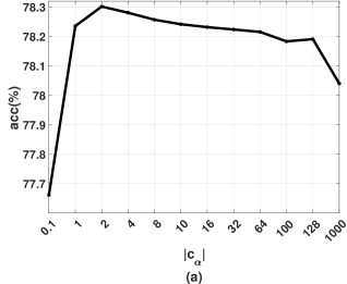
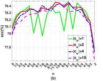
Figure 5: Graphs of classification performance of the SIC model (24) with $\alpha=\alpha_{-}=\alpha_{+}\in[0,2]$. (a) Test accuracy($\%$) vs. ${\left|\,c_{\alpha}\,\right|}$. The test accuracy is the average of all results obtained with $\alpha$ in (39). When ${\left|\,c_{\alpha}\,\right|}=2$, the best performance is achieved. (b) Test accuracy($\%$) vs. $\alpha$. When $\frac{1}{5}\leq{\left|\,\alpha-1\,\right|}\leq 1$, the best performance is achieved with ${\left|\,c_{\alpha}\,\right|}=1$. However, when ${\left|\,\alpha-1\,\right|}<\frac{1}{5}$, the SIC model with ${\left|\,c_{\alpha}\,\right|}\geq 2$ shows better performance.

V Numerical experiments with the $20\times 20$ SIC models

This Section reports the classification results acquired by the SIC model (24) and quasi-Newton(L-BFGS) for virtual convex loss(Algorithm 1 and 2). We compare the proposed methodology with well-known classifiers: $\pi$-weighted convex focal loss [9], LIBLINEAR(logistic regression, SVM, and L2SVM) [26, 32], and LIBSVM(C-SVC with RBF kernel) [41]. Note that Quasi-Newton(L-BFGS) for virtual convex loss is mainly implemented in Matlab(version R2023b) based on [28]. This optimization algorithm is used for the SIC model (24) and the $\pi$-weighted convex focal loss [9]. LIBLINEAR(version 2.4.5) [32] and LIBSVM(version 3.3.2) [41] are mainly implemented in C/C++ language with Matlab interface. All runs are performed on APPLE M2 Ultra with a 24-core CPU and 192GB memory. The operating system is MacOS Sonoma(version 14.1). We use parfor in Matlab for parallel processing of all models, including LIBLINEAR and LIBSVM, in a 24-core CPU. In terms of multi-class datasets, the OVA(one-vs-all) strategy is used for all linear classification models. The OVO(one-vs-one) strategy is used for the kernel-based classification model LIBSVM [41].

Concerning quasi-Newton(L-BFGS) for virtual convex loss, as observed in Figure 4, it is recommended to select $m\in[20,50]$ for two-loop iterations of L-BFGS and $c_{II}\in[0.1,0.5]$ for the interval-based bisection line search(Algorithm 2). We choose $m=40$ and $c_{II}=0.4$ considering performance-computation complexity. For stopping criterions of quasi-Newton(L-BFGS) for virtual convex loss, we use $\|\nabla{\cal F}(h_{t})\|_{\infty}\leq\epsilon_{tol1}$ and $\|h_{t+1}-h_{t}\|_{\infty}\leq\epsilon_{tol2}$ where $\epsilon_{tol1}=10^{-2}$ and $\epsilon_{tol2}=10^{-4}$(Algorithm 1). We could select a smaller $c_{II}$ for exact line search, used in other quasi-Newton optimization, such as nonlinear conjugate gradient [31].

In order to use the $\pi$-weighted convex focal loss [9] discussed in Remark III.6, we need to set three parameters: $\gamma$, $\xi$, and $\pi$. Following the recommendations in [9], we choose $\gamma=1,2,3,4$ and $\xi=0,1$. As for $\pi$, we select $19$ regular points ranging from $0.05$ to $0.95$. This gives us $152$ convex focal losses, expressed as a $(\pi,\gamma:\xi)$-matrix.

We have selected LIBLINEAR [26] and LIBSVM [41] as our standard for balanced linear classification models and non-linear classification models, respectively. For logistic regression, we use logistic loss, hinge-loss for SVM, and squared hinge-loss for L2SVM. To learn an inhomogeneous hyperplane, we set $B=1$. We use the primal formulation ($s=0$) for logistic regression and the dual formulation ($s=3$) for SVM. As for L2SVM, we use the primal formulation ($s=2$). In LIBSVM [41], we use C-SVC(support vector classification) ($s=0$) with the RBF kernel $K(x_{i},x_{j})=\exp(-\nu\|x_{i}-x_{j}\|^{2})$ ($t=2$).

All models have an $\ell_{2}$-regularizer $\frac{\lambda}{2}\|w\|^{2}$. In terms of regularization parameter $\lambda$ for the cost-sensitive learning framework (8), including $20\times 20$ SIC models (24) and $19\times 8$ $\pi$-weighted convex focal loss models in Remark III.6, we use CV(cross-validation) with candidates in (38) as recommended in LIBSVM [41].

$$\lambda=2^{r},\;r=-14,-13,-12,\cdots,5$$ (38)

In LIBLINEAR and LIBSVM, the regularization parameter $\lambda$ is located on the loss function. Therefore, we use $C=\lambda^{-1}$ with (38) for CV. For LIBSVM, in addition to the regularization parameter $C$ on the loss function, the RBF kernel parameter $\nu$ is cross-validated with candidates $\nu=2^{r}$ and $r=-14,..,5$.

Regarding benchmark datasets [8], they are pre-processed and normalized in each feature dimension with mean zero and variance one [7], except for when the variance of the raw data is zero. This process reduces the effect of scale imbalance of datasets. The scale-class-imbalance ratio $r_{sc}$ (1) of two-class and multi-class datasets is presented in Table V and Table VI, respectively. In the case of two-class datasets in Table V, the mean value of $r_{sc}$ of training dataset is ${\bf E}(r_{sc}{\bf T})\approx 1.61$. Also, we have $\min r_{sc}{\bf T}=0.49$ and $\max r_{sc}{\bf T}=7$. Thus, the two-class datasets used in our experiments are roughly well-balanced. However, most of the two-class datasets have variations between $r_{sc}{\bf T}$ and $r_{sc}$ of test dataset ($r_{sc}{\bf Te}$). The raw format of each benchmark dataset is available in the UCI machine learning repository [49]. As commented in [50], we reorganize datasets in [8]. Each dataset is separated into the non-overlapped training and test datasets. The training dataset of each dataset is randomly shuffled for $4$-fold CV [41]. Table V($51$ two-class datasets) and Table VI($67$ multi-class datasets) include all information of datasets such as number of instances, size of training dataset, size of test dataset, feature dimension, number of classes, class-imbalance ratio $r_{c}$ for combined/training/test dataset, and scale-class-imbalance ratio $r_{sc}$ for combined/training/test dataset. The experiments are conducted five times using randomly selected CV datasets, with a fixed initial condition of $(w_{0},b_{0})=(0,0)$. For $\alpha$ and $c_{\alpha}$ of SIC model (24), we conducted a preliminary experiment with the reduced class of SIC model ($\alpha=\alpha_{+}=\alpha_{-}$). We found that the best test classification accuracy is obtainable when ${\left|\,c_{\alpha}\,\right|}=2$. For general purposes, ${\left|\,c_{\alpha}\,\right|}\in[1,10]$ is a possible choice. When $\alpha$ is not close to $1$, the SIC model with ${\left|\,c_{\alpha}\,\right|}=1$ shows the best performance. The detailed information is provided in Figure 5. For the experiments in this Section, we set $c_{\alpha}=2$ for $\alpha>1$ and $c_{\alpha}=-2$ for $\alpha<1$. Thus, $\alpha_{\pm}$ are the only tuning parameters for which we use the following $20$ different values in $[0,2]$:

$$\alpha_{\pm}\in\left\{\;\frac{0}{1},\frac{1}{2},\frac{2}{3},\cdots,\frac{9}{10},\;\frac{11}{10},\frac{10}{9},\frac{9}{8},\cdots,\frac{3}{2},\frac{2}{1}\;\right\}$$ (39)

This gives us $20\times 20$ SIC models. The characteristic of each dataset could be captured by the large class of hyperplanes $h^{*}_{(\alpha_{+},\alpha_{-})}=(w^{*}_{(\alpha_{+},\alpha_{-})},b^{*}_{(\alpha_{+},\alpha_{-})})$ learned via the $20\times 20$ SIC models (24), as noticed in Theorem III.4 and Example III.5. The details are as follows.

MODEL	SIC model(24)				Convex Focal Loss[9]				LIBLINEAR[26]			LIBSVM[41]
SubModel	TOP$1$	MaxA	Max$2$	MaxM	TOP$1$-FL	MaxA-FL	Max$2$-FL	MaxM-FL	Logistic	SVM	L2SVM	C-SVC
$(\alpha_{+},\alpha_{-})$ or $(\pi,\gamma,\xi)$	-	$(\frac{7}{8},\frac{8}{7})$	$(\frac{3}{4},0)$	$(\frac{8}{9},\frac{11}{10})$	-	$(0.5,2,1)$	$(0.5,3,0)$	$(0.6,2,1)$	(primal)	(dual)	(primal)	RBF Kernel
Mean acc($\%$) of Two Class	83.96	82.49	82.51	82.36	83.80	82.14	82.37	81.39	82.11	81.59	82.06	83.22
Mean acc($\%$) of Multi Class	77.30	75.57	75.19	75.57	76.68	75.53	75.36	75.55	74.75	72.94	74.18	79.96
Mean acc($\%$) of All Class	80.18	78.56	78.35	78.50	79.76	78.39	78.39	78.07	77.93	76.68	77.58	81.37
Time of all class	423m	106s	122s	98s	81m	88s	88s	88s	60s	109s	57s	2077m

TABLE II: A comparison of the SIC model (24) with benchmark models: $\pi$-weighted convex focal loss [9], LIBLINEAR [26], and LIBSVM [41]. In this comparison, TOP$1$ refers to a group of SIC models with the best test accuracy for each dataset, while MaxA/Max$2$/MaxM is an SIC model with the best test accuracy for all-, two-, and multi-class. The same notations are used for $\pi$-weighted convex focal loss: TOP$1$-FL, MaxA-FL, Max$2$-FL, and MaxM-FL. In the two-class problems, TOP$1$ performs better than kernel-based LIBSVM and TOP$1$-FL. Max$2$ of the SIC model offers the best test classification accuracy among various linear classifiers. In the multi-class problems, although the SIC model’s TOP$1$ accuracy is less than kernel-based LIBSVM, it still achieves $77.30\%$ accuracy, which is $0.62\%$ better than TOP$1$-FL. When the models’ parameters are fixed, the SIC model performs similarly to the convex focal loss having the external $\pi$-weight parameter.

V-A Performance evaluation of $20\times 20$ SIC models

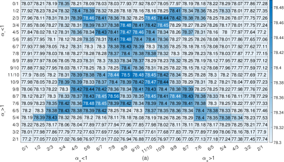
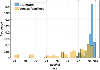
Figure 9: Classification accuracy(%) patterns of all-class are exhibited for (a) $20\times 20$ SIC models and (b) $19\times 8$ convex focal losses. The corresponding histograms are shown in (c). In the case of the SIC model, the best test classification accuracy $78.56\%$ is achieved when $(\alpha_{+},\alpha_{-})=(7/8,8/7)$. On the other hand, the convex focal loss model achieves the best test accuracy $78.39\%$ at $(\pi,\gamma,\xi)=(0.5,3,0),(0.5,2,1)$. Moreover, a histogram comparison between the two models shows that more than half of all SIC models obtain at least $78.20\%$ accuracy, while only $10\%$ of $\pi$-weighted convex focal losses obtain that accuracy.

Table II summarizes the classification accuracy ($\%$) and computation time of all experiments conducted on $118$ datasets. The acronym TOP$1$ refers to a group of SIC models that have the highest test accuracy for each dataset, while MaxA/Max$2$/MaxM refers to an SIC model with the best test accuracy for all-, two-, and multi-class datasets. The same notations are used for $\pi$-weighted convex focal loss: TOP$1$-FL, MaxA-FL, Max$2$-FL, and MaxM-FL. The test classification accuracy of each dataset is reported in Table III for two class datasets and in Table IV for multi-class datasets. Note that MaxA$(\alpha_{+}=\frac{7}{8},\alpha_{-}=\frac{8}{7})$ achieves $78.56\%$. On the other hand, MaxA-FL$(\pi=0.5,\gamma=2,\xi=1)$ obtains $78.39\%$. Over half of all SIC models obtain at least $78.20\%$ accuracy. Out of all the $\pi$-weighted convex focal losses, only $10\%$ can achieve the same level of accuracy as the proposed SIC model. This implies that the SIC model is less sensitive to the parameter than the $\pi$-weighted convex focal loss. Therefore, the SIC model could serve as an alternative cost-sensitive learning framework without external $\pi$-weight. Refer to Figure 9 for additional information. The details are as follows.

In the case of two-class, of which the training dataset is close to the well-balanced condition, TOP$1$ achieves the best results, i.e., $0.74\%$ better than the kernel-based classifier LIBSVM(C-SVC with RBF kernel) and $0.16\%$ better than TOP$1$-FL. When the parameters of the SIC model are fixed, its performance is still better than other linear classifiers, such as $\pi$-weighted convex focal loss and LIBLINEAR. For instance, Max$2$$\left(\alpha_{+}=\frac{3}{4},\alpha_{-}=0\right)$ has $82.51\%$ accuracy, which is $0.14\%$ better than Max$2$-FL and $0.4\%$ better than logistic regression, the best model of LIBLINEAR. As shown in Figure 6 (a), the test accuracy of all SIC models is in the range of $[80.64\%,82.51\%]$. More than $35\%$ of all SIC models achieve at least $82.20\%$ test accuracy. On the other hand, the test accuracy of all convex focal losses is in the range of $[65.93\%,82.37\%]$. Out of all the convex focal loss, only $2\%$ can achieve $82.20\%$ test accuracy. It appears that the SIC models are quite resilient to internal parameter changes. Specifically, Figure 7 (a) shows an ${\bm{X}}$-shaped pattern. This pattern covers a much larger area compared to the best test accuracy area of convex focal losses in Figure 7 (c). The ${\bm{X}}$-shaped pattern relates to the pattern of $\eta$ in Figure 3 (d). It represents a small deviation from the balanced SIC model, which has ${\left|\,\alpha_{+}-1\,\right|}={\left|\,\alpha_{-}-1\,\right|}$. Essentially, the virtual SIGTRON-induced loss functions $L_{\alpha_{+},c_{+}}^{S}$ and $L_{\alpha_{-},c_{-}}^{S}$ of the SIC model have similar polynomial orders, i.e., $k_{+}\approx k_{-}$. Figure 8 (b) horse-colic demonstrates the ${\bm{X}}$-shaped pattern.

It is important to note that spectf dataset in Table V is a typical $r_{sc}$-inconsistent dataset. By using this dataset, the connection between $\eta=\frac{k_{-}}{k_{-}+k_{+}}$ and the movement of the hyperplane $h^{*}_{\alpha_{+},\alpha_{-}}(x)=0$ is empirically demonstrated in Figure 3. Notably, the best test accuracy of the dataset is observed in the region $(\alpha_{+},\alpha_{-})=(-,2)$, which is outside the ${\bm{X}}$-shaped pattern.

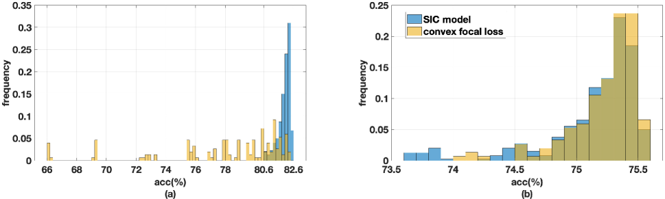
Figure 6: The statistical distributions of $20\times 20$ SIC models and $19\times 8$ convex focal losses with respect to test classification accuracy. (a) The two-class histogram. The SIC models are in the $[80.64\%,82.51\%]$ range, and convex focal losses are in the $[65.93\%,82.37\%]$ range. The SIC model is less sensitive to internal parameters $\alpha_{\pm}$ and outperforms the $\pi$-weighted convex focal losses. (b) The multi-class histogram. The SIC models are in the $[73.64\%,75.57\%]$ range, and convex focal losses are in the $[74.08\%,75.55\%]$ range. Although the SIC models have no external $\pi$-weight parameters, they show comparable performance to $\pi$-weighted convex focal loss. For more information on the matrix pattern of the models, refer to Figure 7.

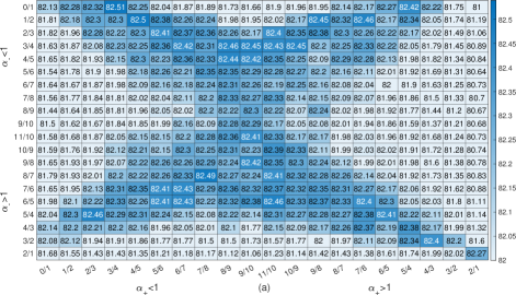
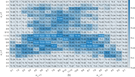
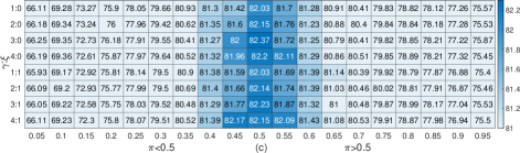
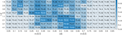
Figure 7: Test accuracy(%) patterns of $20\times 20$ SIC models for (a) two-class and (b) multi-class. Test accuracy(%) patterns of $19\times 8$ convex focal losses for (c) two-class and (d) multi-class. As shown in (a), SIC models exhibit an ${\bm{X}}$-shaped pattern, i.e., ${\left|\,\alpha_{-}-1\,\right|}\approx{\left|\,\alpha_{+}-1\,\right|}$. This indicates that the best-performing SIC models have similar polynomial order between $L_{\alpha_{+},c_{+}}^{S}$ and $L_{\alpha_{-},c_{-}}^{S}$. This ${\bm{X}}$-shaped pattern covers a much larger region than the $\pi$-weighted convex focal losses in (c). For more information and statistical distribution of the models, refer to Figure 6.

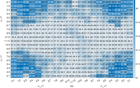
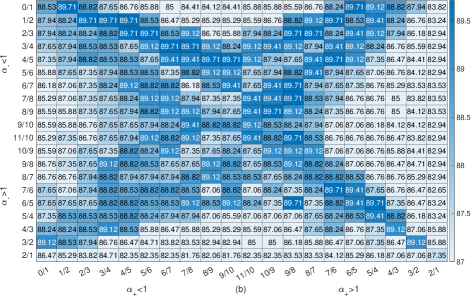
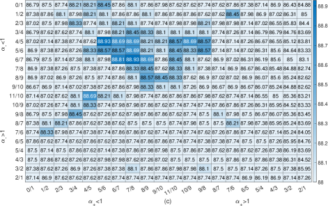
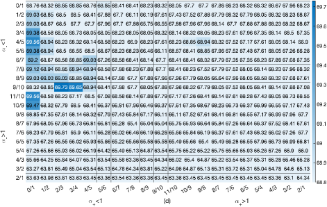
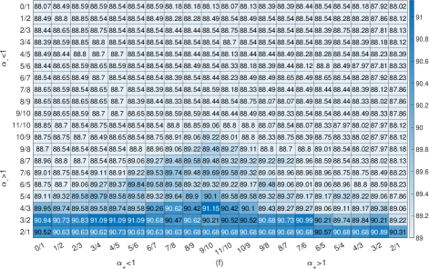
Figure 8: Matrix patterns of the $20\times 20$ SIC models of the test classification accuracy of (a) statlog-australian-credit, (b) horse-colic, (c) ecoli, (d) arrhythmia, (e) energy-y1, and (f) energy-y2. Here statlog-australian-credit and horse-colic are two-class datasets. And ecoli, arrhythmia, energy-y1, and energy-y2 are multi-class datasets. Both energy-y1 and energy-y2 have the same input dataset but look for hyperplanes for opposite outputs, i.e., y1 for the heating load, while y2 for the cooling load [34]. The best performing $(\alpha_{+},\alpha_{-})$ for energy-y1 and energy-y2 exhibit opposite patterns: $(\alpha_{+},\alpha_{-})\approx(2,-)$ for energy-y1, and $(\alpha_{+},\alpha_{-})\approx(-,2)$ for energy-y2. Overall, the best-performing region of multi-class datasets is more localized than that of two-class datasets.

Regarding multi-class datasets, the kernel-based classifier LIBSVM(C-SVC with RBF kernel) achieves the highest test classification accuracy. As presented in Table II, although the test accuracy of TOP$1$ is less than kernel-based LIBSVM, it still achieves a respectable $77.30\%$, which is $0.62\%$ better than TOP$1$-FL. In Figure 6 (b), we observe that the SIC model, which has only internal polynomial order parameters $k_{\pm}=\frac{1}{{\left|\,\alpha_{\pm}-1\,\right|}}$, performs similarly to the convex focal loss, which has the external $\pi$-weight parameter and the internal $\xi$ and $\gamma$ parameters. Note that Figure 7 (b) shows a pattern of the best-performing SIC model in the $(\alpha_{+},\alpha_{-})$-matrix. Compared to two-class, the ${\bm{X}}$-shaped pattern is rounded and biased toward $\alpha_{-}>1$. In the case of convex focal loss in Figure 7 (d), the best-performing region is much larger than the two-class convex focal loss. The region is shifted towards $\pi<0.5$.

Lastly, regarding computation time, L2SVM(primal) and logistic regression(primal) of LIBLINEAR are the fastest models. These models use the truncated Newton method [32] that is based on the unique Hessian structure of the large-margin linear classifier. On the other hand, for both the SIC model and convex focal loss, the proposed Quasi-Newton(L-BFGS) optimization for virtual convex loss is used. As shown in Figure 9 (b) in Appendix -B, the $\pi$-weighted convex focal loss with $\pi=0.5,\gamma=1,\xi=0$, which corresponds to the logistic loss of LIBLINEAR, achieves reasonable performance-computation complexity, resulting in $78.30\%$ test accuracy at $83$ seconds. It is worth noting that the logistic regression of LIBLINEAR only obtains $77.93\%$ test accuracy at $60$ seconds.

Figure 8 demonstrates patterns of test classification accuracy for two-class datasets, statlog-australian-credit and horse-colic and for multi-class datasets, ecoli, arrhythmia, energy-y1, and energy-y2. Overall, the best test accuracy regions of multi-class datasets are more localized than those of two-class datasets. The ${\bm{X}}$-shaped pattern in Figure 7 (a) is also observed in the horse-colic dataset in Figure 8 (b). Both energy-y1 and energy-y2 have the same input dataset but look for hyperplanes for opposite outputs. Specifically, energy-y1 is used to determine the heating load, while energy-y2 is used to determine the cooling load [34]. The best performing $(\alpha_{+},\alpha_{-})$ for energy-y1 and energy-y2 exhibit opposite patterns: $(\alpha_{+},\alpha_{-})\approx(2,-)$ for energy-y1, and $(\alpha_{+},\alpha_{-})\approx(-,2)$ for energy-y2. Refer to Figure 8 (e) and (f) for further details. Understanding the correlation between the pattern of $(\alpha_{+},\alpha_{-})$-matrix and the structure of each dataset can be a valuable tool for multi-label classification and imbalanced classification.

MODEL	SIC model(24)				Convex Focal Loss[9]				LIBLINEAR[26]			LIBSVM[41]
SubModel	TOP$1$	MaxA	Max$2$	MaxM	TOP$1$-FL	MaxA-FL	Max$2$-FL	MaxM-FL	Logistic	SVM	L2SVM	C-SVC
$(\alpha_{+},\alpha_{-})$ or $(\pi,\gamma,\xi)$	-	$(\frac{7}{8},\frac{8}{7})$	$(\frac{3}{4},0)$	$(\frac{8}{9},\frac{11}{10})$	-	$(0.5,2,1)$	$(0.5,3,0)$	$(0.6,2,1)$	(primal)	(dual)	(primal)	RBF Kernel
acute-inflammation	100.00	100.00	100.00	100.00	100.00	100.00	100.00	100.00	100.00	100.00	100.00	100.00
acute-nephritis	100.00	100.00	100.00	100.00	100.00	100.00	100.00	100.00	100.00	100.00	100.00	100.00
adult	84.31	84.24	84.00	84.26	84.38	84.38	84.29	83.73	84.28	84.33	84.05	85.03
balloons	87.50	87.50	87.50	87.50	87.50	87.50	87.50	72.50	87.50	87.50	87.50	87.50
bank	89.00	88.79	88.82	88.81	89.51	88.75	88.81	88.68	88.83	88.19	88.81	88.75
blood	77.17	76.58	76.68	76.15	76.74	75.99	76.20	76.74	76.20	76.20	75.67	76.84
breast-cancer	72.73	72.03	71.61	71.89	73.29	71.61	71.47	72.45	71.05	69.51	70.77	75.66
breast-cancer-wisc	96.85	96.62	96.56	96.62	96.85	96.50	96.33	95.82	96.50	96.62	96.68	95.99
breast-cancer-wisc-diag	98.38	98.17	97.75	98.10	98.31	98.24	98.17	98.24	98.24	97.46	97.96	98.38
breast-cancer-wisc-prog	81.41	79.60	78.59	79.80	82.02	78.79	79.19	79.60	78.38	75.15	79.39	78.38
chess-krvkp	96.93	96.12	96.77	96.46	97.01	96.71	96.53	96.78	96.48	96.33	96.68	98.82
congressional-voting	60.92	58.06	59.17	58.80	61.94	59.26	58.53	60.46	57.70	59.91	57.70	57.33
conn-bench-sonar-mines-rocks	79.23	76.35	75.96	77.88	78.46	75.77	77.12	75.19	75.58	77.50	75.77	84.42
connect-4	75.49	75.45	75.39	75.45	75.50	75.42	75.47	75.38	75.47	75.38	75.41	86.26
credit-approval	89.39	88.58	87.48	89.16	89.62	88.29	88.75	87.36	88.58	87.54	87.88	86.84
cylinder-bands	74.84	73.91	73.28	73.67	74.92	72.42	73.12	71.41	73.83	74.14	73.52	77.34
echocardiogram	86.77	84.92	84.92	84.62	87.38	84.62	84.62	86.15	85.85	87.69	86.15	87.38
fertility	89.60	88.40	88.00	89.60	90.00	84.80	89.60	86.80	85.60	87.20	86.00	86.80
haberman-survival	74.12	73.59	73.59	73.59	74.38	73.59	73.59	72.55	73.86	74.77	73.86	71.63
heart-hungarian	87.89	86.67	86.67	86.67	88.03	85.99	86.53	84.90	86.67	85.03	86.67	86.12
hepatitis	81.04	79.22	77.92	77.66	81.82	75.84	77.40	76.88	77.66	75.06	76.62	81.04
hill-valley	92.08	83.43	92.08	81.39	86.34	81.06	84.75	76.63	80.86	56.70	80.00	65.41
horse-colic	89.71	88.82	87.65	87.35	89.71	88.24	89.41	87.65	87.65	87.06	87.06	85.00
ilpd-indian-liver	73.40	73.40	72.10	72.16	72.58	72.23	71.96	71.55	71.96	71.48	73.06	71.41
ionosphere	88.80	86.29	86.40	86.51	87.09	86.63	86.63	86.97	88.34	87.77	86.74	94.63
magic	79.64	79.12	79.64	79.01	79.45	79.08	79.15	78.20	79.04	78.85	78.97	87.20
miniboone	90.35	90.16	89.77	90.26	90.30	90.30	90.26	90.14	89.79	89.98	89.04	93.50
molec-biol-promoter	84.53	77.36	76.60	76.60	79.25	76.98	77.36	76.60	78.11	76.23	76.23	76.98
mammographic	83.75	83.25	82.96	82.75	83.58	82.87	83.46	83.46	83.50	83.17	83.08	83.21
mushroom	95.24	94.52	95.02	94.60	97.46	95.62	94.58	94.85	94.40	97.64	93.89	100.00
musk-1	84.45	81.93	83.28	82.86	85.46	82.69	82.18	84.87	81.51	83.28	83.19	91.18
musk-2	94.99	94.63	94.56	94.76	95.25	94.80	94.63	95.06	94.67	95.02	94.72	99.19
oocytes-merluccius-nucleus-4d	83.01	82.04	82.04	81.41	82.54	82.07	82.11	81.57	81.80	80.74	82.74	82.07
oocytes-trisopterus-nucleus-2f	81.32	79.91	80.39	79.08	80.88	80.39	78.55	78.42	78.51	78.68	78.73	82.19
ozone	97.22	97.13	97.13	97.08	97.32	97.07	97.11	97.08	97.15	97.10	97.13	96.99
parkinsons	84.12	82.68	82.47	83.09	85.77	83.92	83.09	82.06	82.47	83.51	83.71	91.34
pima	76.98	75.52	75.36	76.61	77.14	76.72	76.61	76.09	76.35	75.31	76.35	73.80
pittsburg-bridges-T-OR-D	89.02	87.84	88.24	88.63	90.20	88.63	88.24	87.84	89.80	86.67	90.20	87.06
planning	70.55	67.47	65.27	67.03	71.43	65.93	67.47	67.91	64.40	70.11	65.27	69.45
ringnorm	77.95	77.37	77.86	77.11	77.87	77.25	76.89	74.16	76.86	77.51	77.11	98.74
spambase	92.88	92.82	92.72	92.44	93.03	92.77	92.45	91.42	92.37	92.78	92.22	93.23
spect	66.67	62.90	62.90	62.26	67.85	61.83	62.04	59.78	64.30	65.16	62.37	60.00
spectf	64.60	56.36	57.86	52.94	61.50	50.48	52.09	46.31	48.98	47.27	49.30	46.84
statlog-australian-credit	68.12	67.13	67.71	66.90	67.94	67.54	67.13	62.55	67.13	67.83	66.96	66.26
statlog-german-credit	77.16	76.96	76.44	76.60	77.40	75.92	76.20	74.96	76.80	76.24	77.16	76.08
statlog-heart	88.59	87.11	86.52	88.00	87.56	87.41	87.26	84.15	86.67	84.59	87.70	84.74
tic-tac-toe	97.91	97.91	97.91	97.91	97.91	97.91	97.91	97.91	97.91	97.91	97.91	98.62
titanic	78.09	77.55	77.55	77.55	78.09	77.55	77.55	77.55	77.55	77.55	77.55	78.42
trains	64.00	60.00	60.00	60.00	60.00	60.00	60.00	60.00	60.00	60.00	60.00	40.00
twonorm	97.66	97.57	97.54	97.56	97.68	97.62	97.44	97.40	97.57	97.49	97.49	97.69
vertebral-column-2clases	85.68	83.23	81.29	82.97	87.61	83.35	83.10	86.06	82.97	81.94	82.32	82.32
Mean	83.96	82.49	82.51	82.36	83.80	82.14	82.37	81.39	82.11	81.59	82.06	83.22

TABLE III: A comparison of two-class test classification accuracy of the SIC model (24) to $\pi$-weighted convex focal loss [9], LIBLINEAR [26], and LIBSVM [41]. Our results indicate that TOP$1$ performs better than kernel-based LIBSVM and the corresponding TOP$1$-FL. Max$2$ offers the best test classification accuracy among various linear classifiers.

MODEL	SIC model(24)				Convex Focal Loss[9]				LIBLINEAR[26]			LIBSVM[41]
SubModel	TOP$1$	MaxA	Max$2$	MaxM	TOP$1$-FL	MaxA-FL	Max$2$-FL	MaxM-FL	Logistic	SVM	L2SVM	C-SVC
$(\alpha_{+},\alpha_{-})$ or $(\pi,\gamma,\xi)$	-	$(\frac{7}{8},\frac{8}{7})$	$(\frac{3}{4},0)$	$(\frac{8}{9},\frac{11}{10})$	-	$(0.5,2,1)$	$(0.5,3,0)$	$(0.6,2,1)$	(primal)	(dual)	(primal)	RBF Kernel
abalone	65.78	65.23	65.43	65.08	65.57	65.31	65.12	65.36	65.18	60.31	65.14	66.22
annealing	87.77	86.27	87.02	86.12	87.12	86.22	85.91	86.97	86.87	87.77	86.97	92.08
arrhythmia	69.73	65.40	68.85	67.88	69.47	68.32	68.76	67.88	68.50	65.93	64.16	67.52
audiology-std	80.00	76.00	78.40	76.00	80.00	72.80	71.20	73.60	70.40	68.80	68.80	65.60
balance-scale	88.46	88.14	88.01	88.27	88.46	88.40	88.14	88.40	88.21	88.21	88.08	98.85
breast-tissue	69.06	66.04	65.28	66.04	66.42	66.42	66.42	66.42	65.28	64.15	66.04	65.66
car	82.64	82.52	81.48	82.41	82.94	82.36	82.36	82.04	82.41	79.93	81.34	98.47
cardiotocography-10clases	79.49	78.46	77.57	78.19	78.74	77.46	77.99	77.84	78.04	73.89	77.38	80.94
cardiotocography-3clases	90.05	89.73	89.56	89.76	90.48	89.78	89.71	89.50	89.84	90.08	89.76	91.95
chess-krvk	28.07	27.83	27.38	27.77	28.10	28.03	27.82	27.96	27.84	17.36	27.59	76.09
conn-bench-vowel-deterding	57.65	52.73	54.24	52.80	55.68	53.26	52.65	54.09	51.89	50.53	54.47	96.06
contrac	51.66	50.98	50.65	50.82	51.22	50.38	50.87	50.49	50.87	46.44	50.03	52.47
dermatology	99.34	97.81	97.38	98.03	98.14	97.60	98.03	98.03	97.81	96.72	97.27	98.14
ecoli	88.93	87.50	88.21	87.74	88.57	88.10	88.21	88.21	87.98	86.07	87.98	85.60
energy-y1	88.85	85.26	85.47	85.57	89.06	85.00	85.57	85.89	86.20	85.16	86.09	94.06
energy-y2	91.15	89.48	88.59	88.85	90.10	88.75	88.23	88.54	89.43	88.85	89.69	92.71
flags	54.85	53.40	53.81	53.40	54.23	52.99	53.20	53.20	52.99	55.05	53.40	53.61
glass	68.22	62.06	63.93	62.80	65.42	64.86	62.80	64.11	63.93	60.00	65.23	70.09
hayes-roth	62.14	53.57	53.57	53.57	57.86	53.57	53.57	53.57	50.71	42.14	45.00	77.14
heart-cleveland	64.11	61.99	62.25	62.52	63.84	62.65	62.65	61.85	61.32	61.19	62.78	59.60
heart-switzerland	41.97	39.34	39.02	39.34	39.67	37.05	38.03	38.03	35.74	37.38	35.74	40.33
heart-va	32.20	29.40	29.40	29.60	32.20	29.60	29.40	29.80	28.20	31.60	27.00	28.00
image-segmentation	91.14	90.13	90.70	90.67	91.30	91.28	90.55	90.89	90.39	90.82	90.18	90.94
iris	97.33	93.33	94.67	94.40	96.00	94.93	94.67	94.67	94.67	91.47	94.40	96.00
led-display	72.12	71.12	70.80	71.56	71.80	70.36	71.32	70.48	70.44	69.16	70.32	69.60
lenses	83.33	75.00	75.00	75.00	75.00	75.00	75.00	75.00	75.00	75.00	75.00	75.00
letter	72.61	72.49	70.06	72.38	72.27	71.95	72.25	72.24	72.22	60.57	70.26	96.53
libras	64.56	61.56	61.78	62.11	65.00	62.56	62.33	62.22	62.67	61.56	61.11	78.22
low-res-spect	89.96	88.15	88.60	88.15	88.83	88.23	87.77	87.55	88.30	88.30	88.23	90.42
lung-cancer	62.50	61.25	57.50	62.50	62.50	62.50	62.50	62.50	57.50	60.00	58.75	56.25
lymphography	84.59	83.24	81.62	83.78	85.14	82.16	82.97	81.89	82.43	82.16	82.43	80.27
molec-biol-splice	84.13	82.98	82.70	82.75	82.81	82.71	82.46	82.62	82.41	81.93	81.98	85.03
nursery	90.64	89.87	89.88	89.84	90.04	89.86	89.86	89.98	89.84	89.51	89.81	99.31
oocytes-merluccius-states-2f	92.41	91.86	92.02	91.94	92.09	91.70	91.74	91.70	91.51	92.02	91.66	91.66
oocytes-trisopterus-states-5b	93.29	92.68	92.85	92.72	92.89	92.76	92.81	92.76	92.50	93.07	92.59	93.60
optical	94.98	94.78	94.64	94.82	95.05	94.92	94.79	94.75	94.74	94.31	94.76	97.28
page-blocks	96.83	96.43	96.21	96.39	96.62	96.24	96.24	96.12	96.29	95.96	96.05	96.64
pendigits	89.86	89.68	89.53	89.38	89.85	89.52	89.54	89.66	89.85	89.47	89.67	97.66
pittsburg-bridges-MATERIAL	88.30	87.92	87.17	86.79	87.55	86.42	86.42	86.79	87.55	88.68	88.68	85.66
pittsburg-bridges-REL-L	69.80	67.45	67.06	67.45	68.63	68.24	63.92	67.84	65.49	66.27	64.31	69.80
pittsburg-bridges-SPAN	79.57	76.09	69.57	74.35	80.00	77.39	74.35	77.39	75.65	74.78	75.22	70.00
pittsburg-bridges-TYPE	65.77	63.85	65.77	62.31	65.38	62.31	62.69	63.46	64.62	58.85	63.46	61.15
plant-margin	78.67	77.70	76.12	77.90	78.53	78.03	78.07	78.00	69.50	58.50	64.80	80.12
plant-shape	55.25	54.22	49.47	54.65	54.62	53.65	53.85	53.40	50.37	40.92	47.10	67.00
plant-texture	80.50	78.15	79.32	78.90	79.77	79.05	78.92	78.97	76.35	70.46	75.02	80.88
post-operative	67.11	66.67	63.56	63.11	66.67	64.89	62.67	64.44	54.67	57.33	55.56	63.11
primary-tumor	49.09	46.55	43.64	45.70	47.76	47.52	45.33	46.55	45.21	41.21	42.42	45.21
seeds	94.29	93.71	93.52	94.29	94.29	93.52	93.71	93.52	92.76	90.48	92.19	91.43
semeion	92.69	92.19	91.56	91.91	92.46	91.48	91.96	91.58	89.12	86.18	85.43	94.65
soybean	86.93	84.84	85.88	85.10	86.80	85.88	84.97	85.62	85.36	88.24	86.67	87.71
statlog-image	93.11	92.28	92.16	92.28	93.65	92.92	92.24	92.31	91.76	91.90	91.26	95.64
statlog-landsat	83.99	82.20	81.30	81.99	81.73	81.58	81.68	81.54	81.91	80.37	81.15	91.89
statlog-shuttle	96.54	93.49	93.41	93.50	94.55	93.88	93.61	93.63	93.12	89.87	92.49	99.90
statlog-vehicle	78.68	77.68	78.53	77.78	79.10	77.73	77.73	77.92	77.78	77.07	77.68	81.89
steel-plates	71.61	71.03	69.75	70.95	71.53	70.76	70.62	70.52	70.47	70.02	70.62	75.03
synthetic-control	97.93	97.27	93.00	97.33	97.73	94.27	96.60	96.07	91.33	87.87	89.20	99.00
teaching	49.60	48.27	46.67	48.53	50.13	48.80	48.80	48.53	48.00	40.80	46.67	52.53
thyroid	96.04	94.75	94.84	94.89	96.06	95.06	95.04	94.99	95.06	95.23	94.46	96.66
vertebral-column-3clases	86.97	85.55	85.16	85.81	86.19	84.52	85.16	83.87	84.00	83.61	84.77	83.35
wall-following	72.85	69.86	69.27	69.77	72.17	69.93	69.52	69.92	69.57	72.89	66.54	90.66
waveform	87.40	86.86	87.09	86.84	87.43	87.08	86.88	87.25	86.66	86.74	86.70	86.92
waveform-noise	86.15	85.86	85.78	85.97	86.06	85.88	86.02	85.86	85.98	85.77	85.90	85.44
wine	98.88	98.43	98.88	98.88	98.88	97.75	98.43	98.20	98.88	98.88	98.65	97.75
wine-quality-red	58.22	57.25	56.52	56.47	58.12	56.42	56.47	56.40	56.85	56.35	56.40	61.20
wine-quality-white	53.87	53.13	53.07	53.32	54.02	53.74	53.51	54.02	53.56	47.10	53.27	60.21
yeast	60.75	59.95	59.65	59.62	61.11	60.49	60.19	60.38	60.16	52.26	59.97	60.75
zoo	96.00	96.00	96.00	96.00	96.00	96.00	96.00	96.00	96.00	95.60	96.00	96.00
Mean	77.30	75.57	75.19	75.57	76.68	75.53	75.36	75.55	74.75	72.94	74.18	79.96

TABLE IV: A comparison of multi-class test classification accuracy of the SIC model (24) to $\pi$-weighted convex focal loss [9], LIBLINEAR [26], and LIBSVM [41]. Although the accuracy of TOP$1$ is less than kernel-based LIBSVM, it still achieves $77.30\%$ accuracy, which is $0.62\%$ better than TOP$1$-FL. Within linear classifiers, the SIC model performs similarly to the convex focal loss having the external $\pi$-weight parameter, i.e., MaxM achieves $75.57\%$ vs. MaxM-FL achieves $75.55\%$.

VI Conclusion

This article introduces SIGTRON, an extended asymmetric sigmoid function with Perceptron, and its virtualized loss function called virtual SIGTRON-induced loss function. Based on this loss function, we propose the SIGTRON-imbalanced classification (SIC) model for cost-sensitive learning. Unlike other models, the SIC model does not use an external $\pi$-weight on the loss function but instead has an internal two-dimensional parameter $(\alpha_{+},\alpha_{-})$-matrix. We show that when a training dataset is close to a well-balanced condition, the SIC model is moderately resilient to variations in the dataset through the skewed hyperplane equation. When $r_{sc}$ is not severe, the proposed SIC model could be used as an alternative cost-sensitive learning model that does not require an external $\pi$-weight parameter. Additionally, we introduce quasi-Newton(L-BFGS) optimization for virtual convex loss with an interval-based bisection line search. This optimization is a competitive framework for a convex minimization problem, compared to conventional L-BFGS with cubic-interpolation-based line search. We utilize the proposed optimization framework for the SIC model and the $\pi$-weighted convex focal loss. Our SIC model has shown better performance in terms of test classification accuracy with 118 diverse datasets compared to the $\pi$-weighted convex focal loss and LIBLINEAR. In binary classification problems, where the severity of $r_{sc}$ is not high, selecting the best SIC model for each dataset(TOP$1$) can lead to better performance than the kernel-based LIBSVM. Specifically, TOP$1$ achieves a test classification accuracy of $83.96\%$, which is $0.74\%$ better than the accuracy of LIBSVM and $0.16\%$ better than the accuracy of TOP$1$-FL of the convex focal loss. In multi-class classification problems, although the test accuracy of TOP$1$ is lower than that of kernel-based LIBSVM, it achieves an accuracy of $77.30\%$, which is $0.62\%$ better than the accuracy of TOP$1$-FL of the convex focal loss. Last but not least, the proposed SIC model, which includes an $(\alpha_{+},\alpha_{-})$-matrix parameter, could be a valuable tool for analyzing various structures of datasets, such as $r_{sc}$-inconsistency and multi-label structures.

-A Proof of Theorem II.2

Let $\alpha=1$, then we have $s_{\alpha,c}(x)=\frac{1}{1+\exp(-x)}\in C^{\infty}({\mathbb{R}})$. Therefore, we only consider the case $\alpha\not=1$. Note that $\nabla^{n}s_{\alpha,c}(x)=0$, for all $x\in{\mathbb{R}}\setminus\hbox{dom}(\sigma_{\alpha,c})$ and $n=1,2,3,\cdots$. Also, for $x\in int(\hbox{dom}(\sigma_{\alpha,c}))$, let $y=1+\frac{x}{c_{\alpha}}>0$ and $a=\frac{1}{1-\alpha}$, then we get $s_{\alpha,c}(c_{\alpha}(y-1))=\frac{1}{1+y^{a}}$. Thus, it is not difficult to see $s_{\alpha,c}(x)=\sigma_{\alpha,c}(x)\in C^{\infty}(int(\hbox{dom}(\sigma_{\alpha,c})))$.

For the continuity of $\nabla^{n}s_{\alpha,c}(x)$ on $x\in{\mathbb{R}}$, we only need to check $s_{\alpha,c}(-c_{\alpha})=0$. Let us assume that (13) is true. (A) When $0\leq\alpha<1$, $\exp_{\alpha,c}(-x)=0$ at $x=-c_{\alpha}$. Thus, we only need to consider numerator of $F_{n,k}(x)$, i.e., $(\exp_{\alpha,c}(-x))^{k-n(1-\alpha)}$. $F_{n,k}(c_{\alpha})=0$, if $k-n(1-\alpha)>0$ for all $k=1,2,\cdots,n$. Now, we get $1>\alpha>1-1/n$. (B) When $\alpha>1$, $\exp_{\alpha,c}(-x)=+\infty$ at $x=-c_{\alpha}$. Thus, we have $F_{n,k}(-c_{\alpha})=\lim_{x\rightarrow-c_{\alpha}}cA_{n,k}\left(\frac{1}{1-\alpha}\right)(\exp_{\alpha,c}(-x))^{-n(1-\alpha)-1}=0$ if $-n(1-\alpha)-1<0$. It means $1<\alpha<1+1/n$. From (A) and (B), we get $\nabla^{n}s_{\alpha,c}(x)\in C^{n}({\mathbb{R}})$ for $\alpha\in\left(1-\frac{1}{n},1+\frac{1}{n}\right)$.

Now, we want to show (13) by induction for $x\in int(\hbox{dom}(\sigma_{\alpha,c}))$. Let $y=1+\frac{x}{c_{\alpha}}$ and $a=\frac{1}{1-\alpha}$, then (13) becomes

$$\frac{d^{n}}{dy^{n}}\frac{1}{1+y^{a}}=\sum_{k=1}^{n}B_{n,k}(a)\frac{y^{ka-n}}{(1+y^{a})^{k+1}}$$ (40)

where $B_{n,k}(a)=(-1)^{n+k}k!\sum_{l=0}^{n}{\left[n\atop l\right]}{\left\{l\atop k\right\}}(-a)^{l}$.

(I) Let $n=1$. Then the left-hand side of (40) is $\frac{d}{dy}\frac{1}{1+y^{a}}=\frac{-ay^{a-1}}{(1+y^{a})^{2}}$. The right-hand side is $B_{1,1}(a)\frac{x^{a-1}}{(1+x^{a})^{2}}$ where $B_{1,1}(a)=\left[1\atop 0\right]\left\{0\atop 1\right\}+\left[1\atop 1\right]\left\{1\atop 1\right\}(-a)=-a$. For the computation of the Stirling number of the first and second kind, we use the following convention and rule in [42]: $\left\{0\atop 0\right\}=\left[0\atop 0\right]=1$ and $\left\{a\atop 0\right\}=\left[a\atop 0\right]=0$ for $a\geq 1$. Also, we have $\left\{a\atop 1\right\}=1$ and $\left[a\atop 1\right]=(a-1)!$ with $0!=1$, for $a\geq 1$. Additionally, $\left\{a\atop b\right\}=\left[a\atop b\right]=0$ if $b>a\geq 0$.

(II) For $n>1$, let (40) be true. Then, for $n+1$, we need to show that

$$\frac{d}{dy}\left(\sum_{k=1}^{n}B_{n,k}(a)\frac{y^{ak-n}}{(1+y^{a})^{k+1}}\right)=\sum_{k=1}^{n+1}B_{n+1,k}(a)\frac{y^{ak-(n+1)}}{(1+y^{a})^{k+1}},$$ (41)

where

$$\frac{d}{dy}\left(\sum_{k=1}^{n}B_{n,k}(a)\frac{y^{ak-n}}{(1+y^{a})^{k+1}}\right)=\sum_{k=1}^{n}B_{n,k}(a)\left(\frac{(ak-n)y^{ak-(n+1)}}{(1+y^{a})^{k+1}}-(k+1)\frac{ay^{a(k+1)-(n+1)}}{(1+y^{a})^{k+2}}\right).$$ (42)

From (41) and (42), we get

$$B_{n+1,k}(a)=(-ka)B_{n,k-1}(a)+(ka-n)B_{n,k}(a)$$ (43)

where $B_{n,0}(a)=B_{n,n+1}(a)=0$. It comes from the rule of the Stirling number in (I). Now, we only need to prove (43). The left-hand side of (43) is

$$B_{n+1,k}(a) = (-1)^{k}k!\sum_{l=0}^{n+1}\left[n+1\atop l\right]\left\{l\atop k\right\}(-1)^{n+1-l}a^{l}$$

$$= (-1)^{k}k!\left(\left\{n+1\atop k\right\}a^{n+1}+\sum_{l=1}^{n}\left(n\left[n\atop l\right]+\left[n\atop l-1\right]\right)\left\{l\atop k\right\}(-1)^{n+1-l}a^{l}\right)$$

where $\left[n+1\atop 0\right]=0$, $\left[n+1\atop n+1\right]=1$, and $\left[n+1\atop l\right]=n\left[n\atop l\right]+\left[n\atop l-1\right]$(see the rule of the Stirling number in (I) and [42]). By using the equivalence $\left\{l+1\atop k\right\}=\left\{l\atop k-1\right\}+k\left\{l\atop k\right\}$ and $\left[n\atop 0\right]=0$, the right-hand side of (43) is simplified to the following equation.

$$(-ka)B_{n,k-1}(a)+(ka-n)B_{n,k}(a)=(-1)^{k}k!\sum_{l=0}^{n}\left(a\left\{l+1\atop k\right\}-n\left\{l\atop k\right\}\right)\left[n\atop l\right](-1)^{n-l}a^{l}.$$

By dividing $(-1)^{k}k!$ and adding $\sum_{l=1}^{n}n\left[n\atop l\right]\left\{l\atop k\right\}(-1)^{n-l}a^{l}$ on both sides, we obtain the equivalence (43).

-B The structure of the dataset and classification results of all-class

We summarize the structure of $118$ datasets used in our experiments and present classification accuracy of the SIC model and $\pi$-weighted convex focal loss of all-class. Table V summarizes two-class datasets. For each dataset, we describe the number of instances, the size of training dataset, the size of test dataset, the size of class, and the feature dimension. Additionally, we show imbalancedness, i.e., $r_{c}/r_{c}{\bf T}/r_{c}{\bf Te}$ for class-imbalance ratio of combined/training/test dataset and $r_{sc}/r_{sc}{\bf T}/r_{sc}{\bf Te}$ for scale-class-imbalance ratio of combined/training/test dataset. Table VI summarizes multi-class datasets. For each dataset, we describe the number of instances, the size of training dataset, the size of test dataset, the feature dimension, and the size of class. Additionally, we show imbalancedness, i.e., minimum and maximum of $r_{c}$ for combined/training dataset: $r_{c}{\bf m}/r_{c}{\bf M}/r_{c}{\bf Tm}/r_{c}{\bf TM}$. Also, minimum and maximum of $r_{sc}$ for combined/training dataset: $r_{sc}{\bf m}/r_{sc}{\bf M}/r_{sc}{\bf Tm}/r_{sc}{\bf TM}$.

Figure 9 presents classification accuracy matrix and the corresponding histogram of all-class for $20\times 20$ SIC models and $19\times 8$ convex focal losses. The test classification accuracy of all SIC models ranges between $76.88\%$ and $78.56\%$. On the other hand, the test classification accuracy of all convex focal losses ranges between $71.04\%$ and $78.39\%$.

	instance	train	test	dim	class	$r_{c}$	$r_{sc}$	$r_{c}$T	$r_{sc}$T	$r_{c}$Te	$r_{sc}$Te
acute-inflammation	120	60	60	6	2	1.03	1.01	1	0.95	1.07	1.06
acute-nephritis	120	60	60	6	2	1.40	1.14	1.40	1.14	1.40	1.14
adult	48842	32561	16281	14	2	3.18	2.10	3.15	2.09	3.23	2.14
balloons	16	8	8	4	2	1.29	1.18	1	0.72	1.67	2.15
bank	4521	2261	2260	16	2	7.68	4.43	7.66	4.38	7.69	4.45
blood	748	374	374	4	2	3.20	2.63	3.20	2.41	3.20	2.80
breast-cancer	286	143	143	9	2	2.36	1.92	2.33	1.91	2.40	1.89
breast-cancer-wisc	699	350	349	9	2	1.90	1.12	1.89	1.13	1.91	1.11
breast-cancer-wisc-diag	569	285	284	30	2	1.68	1.06	1.69	0.99	1.68	1.14
breast-cancer-wisc-prog	198	99	99	33	2	3.21	2.06	3.12	2.42	3.30	1.98
chess-krvkp	3196	1598	1598	36	2	0.91	0.95	0.92	0.97	0.91	0.95
congressional-voting	435	218	217	16	2	1.59	1.53	1.60	1.54	1.58	1.51
conn-bench-sonar-mines-rocks	208	104	104	60	2	1.14	1.04	1.12	1.02	1.17	1.06
connect-4	67557	33779	33778	42	2	3.06	2.94	3.06	2.95	3.06	2.92
credit-approval	690	345	345	15	2	0.80	0.90	0.81	0.99	0.80	0.83
cylinder-bands	512	256	256	35	2	0.64	0.75	0.64	0.79	0.64	0.74
echocardiogram	131	66	65	10	2	2.05	1.47	2	1.52	2.10	1.44
fertility	100	50	50	9	2	7.33	5.47	7.33	4.96	7.33	6.07
haberman-survival	306	153	153	3	2	2.78	2.53	2.73	2.22	2.83	2.79
heart-hungarian	294	147	147	12	2	1.77	1.26	1.77	1.37	1.77	1.17
hepatitis	155	78	77	19	2	0.26	0.52	0.26	0.65	0.26	0.44
hill-valley	606	303	303	100	2	1.03	1.03	1.02	0.84	1.03	0.83
horse-colic	368	300	68	25	2	1.71	1.30	1.75	1.31	1.52	1.22
ilpd-indian-liver	583	292	291	9	2	2.49	2.04	2.48	2.07	2.51	2.06
ionosphere	351	176	175	33	2	0.56	0.81	0.56	0.86	0.56	0.83
magic	19020	9510	9510	10	2	1.84	1.51	1.84	1.51	1.84	1.52
miniboone	130064	65032	65032	50	2	0.39	0.55	0.39	0.55	0.39	0.55
molec-biol-promoter	106	53	53	57	2	1	1	0.96	1.01	1.04	0.99
mammographic	961	481	480	5	2	1.16	1.09	1.16	1.11	1.16	1.06
mushroom	8124	4062	4062	21	2	1.07	1.03	1.07	1.05	1.07	1
musk-1	476	238	238	166	2	1.30	1.07	1.29	1.53	1.31	0.93
musk-2	6598	3299	3299	166	2	5.49	1.74	5.48	1.78	5.49	1.73
oocytes-merluccius-nucleus-4d	1022	511	511	41	2	0.49	0.59	0.49	0.55	0.49	0.62
oocytes-trisopterus-nucleus-2f	912	456	456	25	2	0.73	0.79	0.73	0.85	0.73	0.71
ozone	2536	1268	1268	72	2	33.74	6.98	33.27	7	34.22	7.31
parkinsons	195	98	97	22	2	0.33	0.73	0.32	0.92	0.33	0.56
pima	768	384	384	8	2	1.87	1.53	1.87	1.51	1.87	1.53
pittsburg-bridges-T-OR-D	102	51	51	7	2	6.29	4.10	6.29	4.71	6.29	3.41
planning	182	91	91	12	2	2.50	2.46	2.50	2.39	2.50	2.45
ringnorm	7400	3700	3700	20	2	0.98	0.99	0.98	1	0.98	0.98
spambase	4601	2301	2300	57	2	1.54	1.16	1.54	1.16	1.54	1.17
spect	265	79	186	22	2	1.41	1.21	2.04	1.41	1.21	1.11
spectf	267	80	187	44	2	0.26	0.52	1	1	0.09	0.26
statlog-australian-credit	690	345	345	14	2	0.47	0.49	0.47	0.49	0.47	0.48
statlog-german-credit	1000	500	500	24	2	2.33	1.82	2.33	1.81	2.33	1.84
statlog-heart	270	135	135	13	2	1.25	1.09	1.25	1.15	1.25	1.02
tic-tac-toe	958	479	479	9	2	0.53	0.60	0.53	0.61	0.53	0.59
titanic	2201	1101	1100	3	2	2.10	1.76	2.09	1.75	2.10	1.77
trains	10	5	5	29	2	1	1	0.67	0.70	1.50	1.21
twonorm	7400	3700	3700	20	2	1	1	1	1	1	1
vertebral-column-2clases	310	155	155	6	2	2.10	1.56	2.10	1.51	2.10	1.63

TABLE V: Two-class datasets in [8, 50]. Note that $r_{c}$ is the class-imbalance ratio and $r_{sc}$ is the scale-class-imbalance ratio defined in (1). Additionally, $r_{c}$T and $r_{sc}$T (or $r_{c}$Te and $r_{sc}$Te) are $r_{c}$ and $r_{sc}$ of training dataset (or test dataset).

	inst.	train	test	dim	cls	$r_{c}$m	$r_{c}$M	$r_{sc}$m	$r_{sc}$M	$r_{c}$Tm	$r_{c}$TM	$r_{sc}$Tm	$r_{sc}$TM
abalone	4177	2089	2088	8	3	0.46	0.53	0.53	0.82	0.46	0.53	0.54	0.82
annealing	798	399	399	31	5	0.01	3.20	0.06	2.06	0.01	3.20	0.11	2.12
arrhythmia	452	226	226	262	13	0	1.18	0.05	1.04	0	1.11	0.06	1.02
audiology-std	196	171	25	59	18	0.01	0.32	0.05	0.59	0.01	0.36	0.05	0.59
balance-scale	625	313	312	4	3	0.09	0.85	0.09	0.91	0.09	0.85	0.09	0.94
breast-tissue	106	53	53	9	6	0.15	0.26	0.31	0.71	0.15	0.26	0.27	0.58
car	1728	864	864	6	4	0.04	2.34	0.08	1.77	0.04	2.32	0.08	1.79
cardiotocography-10clases	2126	1063	1063	21	10	0.03	0.37	0.07	0.55	0.03	0.37	0.07	0.54
cardiotocography-3clases	2126	1063	1063	21	3	0.09	3.51	0.34	1.85	0.09	3.50	0.31	1.89
chess-krvk	28056	14028	14028	6	18	0	0.19	0	0.24	0	0.19	0	0.24
conn-bench-vowel-deterding	528	264	264	11	11	0.10	0.10	0.11	0.25	0.10	0.10	0.12	0.26
contrac	1473	737	736	9	3	0.29	0.75	0.37	0.78	0.29	0.74	0.39	0.77
dermatology	366	183	183	34	6	0.06	0.44	0.39	0.90	0.06	0.43	0.40	0.87
ecoli	336	168	168	7	8	0.01	0.74	0.01	0.89	0.01	0.71	0.01	0.84
energy-y1	768	384	384	8	3	0.22	0.88	0.31	0.97	0.22	0.87	0.29	0.99
energy-y2	768	384	384	8	3	0.33	0.99	0.58	1	0.33	0.99	0.60	0.95
flags	194	97	97	28	8	0.02	0.45	0.06	0.68	0.02	0.43	0.05	0.66
glass	214	107	107	9	6	0.04	0.55	0.11	0.60	0.05	0.51	0.10	0.57
hayes-roth	160	132	28	3	3	0.24	0.68	0.40	0.74	0.29	0.63	0.46	0.69
heart-cleveland	303	152	151	13	5	0.04	1.18	0.11	1.07	0.05	1.14	0.14	1.14
heart-switzerland	123	62	61	12	5	0.04	0.64	0.06	0.67	0.05	0.63	0.08	0.66
heart-va	200	100	100	12	5	0.05	0.39	0.10	0.46	0.05	0.37	0.09	0.48
image-segmentation	2310	210	2100	18	7	0.17	0.17	0.27	0.69	0.17	0.17	0.27	0.69
iris	150	75	75	4	3	0.50	0.50	0.58	0.82	0.50	0.50	0.56	0.84
led-display	1000	500	500	7	10	0.09	0.12	0.18	0.30	0.09	0.13	0.19	0.29
lenses	24	12	12	4	3	0.20	1.67	0.35	1.37	0.20	1.40	0.35	1.39
letter	20000	10000	10000	16	26	0.04	0.04	0.06	0.14	0.04	0.04	0.06	0.14
libras	360	180	180	90	15	0.07	0.07	0.12	0.54	0.07	0.07	0.13	0.51
low-res-spect	531	266	265	100	9	0	1.08	0.05	1.01	0	1.06	0.04	0.98
lung-cancer	32	16	16	56	3	0.39	0.68	0.78	0.87	0.45	0.60	0.72	0.87
lymphography	148	74	74	18	4	0.01	1.21	0.08	1.10	0.01	1.18	0.08	1.04
molec-biol-splice	3190	1595	1595	60	3	0.32	1.08	0.51	1.05	0.32	1.08	0.51	1.07
nursery	12960	6480	6480	8	5	0	0.50	0	0.67	0	0.50	0	0.67
oocytes-merluccius-states-2f	1022	511	511	25	3	0.06	2.19	0.37	1.14	0.06	2.17	0.37	1.07
oocytes-trisopterus-states-5b	912	456	456	32	3	0.02	1.36	0.08	1.04	0.02	1.35	0.09	1.08
optical	5620	3823	1797	62	10	0.11	0.11	0.30	0.51	0.11	0.11	0.31	0.53
page-blocks	5473	2737	2736	10	5	0.01	8.77	0.06	4.07	0.01	8.74	0.06	4.01
pendigits	10992	7494	3498	16	10	0.11	0.12	0.23	0.44	0.11	0.12	0.25	0.44
pittsburg-bridges-MATERIAL	106	53	53	7	3	0.12	2.93	0.20	1.67	0.13	2.79	0.29	1.37
pittsburg-bridges-REL-L	103	52	51	7	3	0.17	1.06	0.24	1.04	0.18	1	0.25	1.20
pittsburg-bridges-SPAN	92	46	46	7	3	0.31	1.09	0.45	1.07	0.31	1.09	0.39	1.08
pittsburg-bridges-TYPE	105	53	52	7	6	0.11	0.72	0.14	0.78	0.10	0.66	0.17	0.79
plant-margin	1600	800	800	64	100	0.01	0.01	0.03	0.14	0.01	0.01	0.03	0.14
plant-shape	1600	800	800	64	100	0.01	0.01	0.01	0.25	0.01	0.01	0.01	0.25
plant-texture	1599	800	799	64	100	0.01	0.01	0.03	0.11	0.01	0.01	0.03	0.12
post-operative	90	45	45	8	3	0.02	2.46	0.06	2.31	0.02	2.46	0.06	1.95
primary-tumor	330	165	165	17	15	0.02	0.34	0.04	0.55	0.02	0.32	0.04	0.50
seeds	210	105	105	7	3	0.50	0.50	0.65	0.86	0.50	0.50	0.69	0.87
semeion	1593	797	796	256	10	0.11	0.11	0.52	0.74	0.11	0.11	0.52	0.69
soybean	307	154	153	35	18	0.01	0.15	0.10	0.49	0.01	0.15	0.10	0.49
statlog-image	2310	1155	1155	18	7	0.17	0.17	0.27	0.69	0.17	0.17	0.27	0.68
statlog-landsat	6435	4435	2000	36	6	0.11	0.31	0.26	0.83	0.10	0.32	0.25	0.84
statlog-shuttle	58000	43500	14500	9	7	0	3.67	0	1.67	0	3.63	0	1.67
statlog-vehicle	846	423	423	18	4	0.31	0.35	0.48	0.62	0.31	0.35	0.35	0.72
steel-plates	1941	971	970	27	7	0.03	0.53	0.09	0.76	0.03	0.53	0.10	0.71
synthetic-control	600	300	300	60	6	0.20	0.20	0.28	0.85	0.20	0.20	0.29	0.87
teaching	151	76	75	5	3	0.48	0.53	0.53	0.58	0.49	0.52	0.54	0.54
thyroid	7200	3772	3428	21	3	0.02	12.48	0.08	5.19	0.03	12.28	0.08	4.96
vertebral-column-3clases	310	155	155	6	3	0.24	0.94	0.43	0.98	0.24	0.94	0.43	0.92
wall-following	5456	2728	2728	24	4	0.06	0.68	0.24	0.78	0.06	0.68	0.23	0.80
waveform	5000	2500	2500	21	3	0.49	0.51	0.75	0.85	0.49	0.51	0.74	0.85
waveform-noise	5000	2500	2500	40	3	0.49	0.51	0.76	0.84	0.49	0.51	0.77	0.86
wine	178	89	89	13	3	0.37	0.66	0.78	0.87	0.37	0.65	0.76	0.89
wine-quality-red	1599	800	799	11	6	0.01	0.74	0.02	0.81	0.01	0.74	0.02	0.81
wine-quality-white	4898	2449	2449	11	7	0	0.81	0	0.82	0	0.81	0	0.82
yeast	1484	742	742	8	10	0	0.45	0.03	0.51	0	0.45	0.03	0.51
zoo	101	51	50	16	7	0.04	0.68	0.13	0.93	0.04	0.65	0.13	0.91

TABLE VI: Multi-class datasets in [8, 50]. Here, $0$ means $<0.01$. Note that $r_{c}$m/M is the minimum/maximum class-imbalance ratio of datasets and $r_{sc}$m/M is the minimum/maximum scale-class-imbalance ratio defined in (1). Additionally, $r_{c}$Tm/M and $r_{sc}$Tm/M are the corresponding imbalance ratios for training datasets. OVA strategy is used for $r_{c}$ and $r_{sc}$.

References

- [1] A. Fernández, S. García, M. Galar, R. C. Prati, B. Krawczyk, and F. Herrera, Learning from imbalanced datasets, Springer-Verlag, 2018.
- [2] J. M. Johnson and T. M. Khoshgoftaar, “Survey on deep learning with class imbalance”, Journal of Big Data, vol. 6, pp. 1-54., 2019.
- [3] K. Oksuz, B. C. Cam, S. Kalkan, and E. Akbas, “Imbalance problems in object detection: a review”, IEEE Transactions on Pattern Analysis and Machine Intelligence, vol. 43, pp. 3388-3415, 2021.
- [4] F. R. Bach, D. Heckerman, and E. Horvitz, “Considering cost asymmetry in learning classifiers,”, Journal of Machine Learning Research, vol. 7, pp. 1713-1741, 2006.
- [5] H. He and E. A. Garcia, “Learning from imbalanced data”, IEEE Transactions on Knowledge and Data Engineering, vol. 21, pp. 1263-1284, 2009.
- [6] S. Garcia, J. Luengo, and F. Herrera, Data preprocessing in data mining. Springer-Verlag, 2015.
- [7] S. Ioffe and C. Szegedy, “Batch normalization: Accelerating deep network training by reducing internal covariate shift”, arXiv:1502.03167v3, 2015.
- [8] M. F.-Delgado, E. Cernadas, S. Barro, and D. Amorim, “Do we need hundreds of classifiers to solve real world classification problems?”, Journal of Machine Learning Research, vol. 15, pp. 3133-3181, 2014.
- [9] T.-Y. Lin, P. Goyal, R. Girshick, K. He, and P. Dollár, “Focal loss for dense object detection”, IEEE Transactions on Pattern Analysis and Machine Intelligence, vol. 42, pp. 318-327, 2020.
- [10] H. Masnadi-Shirazi and N. Vasconcelos, “On the design of loss functions for classification: theory, robustness to outliers, and savageboost”, Advances in Neural Information Processing Systems 21, 2008.
- [11] M. D. Reid and R. C. Williamson, “Information, divergence and risk for binary experiments”, Journal of Machine Learning Research, vol. 12, pp. 731-817, 2011.
- [12] A. F. T. Martins and R. F. Astudillo, “From softmax to sparsemax: A sparse model of attention and multi-label classification”, Proceedings of the 33th International Conference on Machine Learning, 2016.
- [13] Y. Ollivier, “Riemannian metrics for neural networks I: feedforward networks”, Information and Inference: A Journal of the IMA, vol. 4. pp. 108-153, 2015.
- [14] A. de Brébisson and P. Vincent, “An exploration of softmax alternatives belonging to the spherical loss family”, arXiv:1511.05042v3, 2016.
- [15] H. Woo, “Logitron: Perceptron-augmented classification model based on an extended logistic loss function”, arXiv:1904.02958v1, 2019.
- [16] S. R. Dubey, S. K. Singh, and B. B. Chaudhuri, “Activation functions in deep learning: A comprehensive survey and benchmark”, arXiv:2109.14545v3, 2022.
- [17] Wikipedia - sigmoid function https://en.wikipedia.org/wiki/Sigmoid_function.
- [18] K. P. Murphy, Machine Learning, MIT Press, 2012.
- [19] P. McCullagh and J. A. Nelder, Generalized Linear Models, Second Edition, Chapman & Hall/CRC, 1989.
- [20] R. Wedderburn, “Quasi-likelihood functions, generalized linear models, and the Gauss-Newton method”, Biometrika, vol. 61, pp. 439-447, 1974.
- [21] H. Woo, “Bregman-divergence-guided Legendre exponential dispersion model with finite cumulants (-LED)”, arXiv: 1910.03025v1, 2019.
- [22] J. Liao, O. Kosut, L. Sankar, F. du Pin Calmon, “Tunable measures for information leakage and applications to privacy-utility tradeoffs”, IEEE Transactions on Information Theory, vol. 65, pp. 8043-8066, 2019.
- [23] T. Sypherd, M. Diaz, J. K. Cava, G. Dasarathy, P. Kairouz, and L. Sankar, “A tunable loss function for robust classification: calibration, landscape, and generalization”, IEEE Transactions on Information Theory, vol. 68, pp. 6021-6051, 2022.
- [24] Y. Lin, “Support Vector Machines and the Bayes rule in classification”, Data Mining and Knowledge Discovery, vol. 6, pp. 259-275, 2002.
- [25] K. Janocha and W. M. Czarnecki, “On loss functions for deep neural networks in classification”, arXiv:1702.05659v1, 2017.
- [26] R.-E. Fan, K.-W. Chang, C.-J. Hsieh, X.-R. Wang, and C.-J. Lin, ”LIBLINEAR: A library for large linear classification”, Journal of Machine Learning Research, vol. 9, pp. 1871-1874, 2008.
- [27] J. Nocedal and S. J. Wright, Numerical Optimization, Second Edition, Springer-Verlag, 2006.
- [28] M. Schmidt, minFunc: unconstrained differentiable multivariate optimization in Matlab, http://www.cs.ubc.ca/~schmidtm/Software/minFunc.html, 2005.
- [29] M. Mutschler and A. Zell, “Parabolic approximation line search for DNNs”, Advances in Neural Information Processing Systems 33, 2020.
- [30] W. W. Hager and H. Zhang, “Algorithm 851: CG_DESCENT, a conjugate gradient method with guaranteed descent”, ACM Transactions on Mathematical Software, vol. 32, pp. 113-137, 2006.
- [31] W. W. Hager and H. Zhang, “A new conjugate gradient method with guaranteed descent and an efficient line search”, SIAM Journal on Optimization, vol. 16, pp. 170-192, 2005.
- [32] L. Galli and C.-J. Lin, “A study on truncated Newton methods for linear classification”, IEEE Transactions on Neural Networks and Learning Systems, vol. 33, pp. 2828-2841, 2022.
- [33] L. A. Kurgan, K. J. Cios, R. Tadeusiewicz, M. Ogiela, L. Goodenday, “Knowledge discovery approach to automated cardiac SPECT diagnosis,”, Artificial Intelligence in Medicine, vol. 23, pp. 149-169, 2001.
- [34] A. Tsanas and A. Xifara, “Accurate quantitative estimation of energy performance of residential building using statistical machine learning tools,”, Energy Buildings, vol. 49, pp. 560-567, 2012.
- [35] H. Woo, “The Bregman-Tweedie classification model”, arXiv: 1907.06923v1, 2019.
- [36] H. Woo, “A characterization of the domain of Beta-divergence and its connection to Bregman variational model”, Entropy, vol. 19, 482, 2017.
- [37] B. Jorgensen, The Theory of Dispersion Models, Chapman & Hall, 1997.
- [38] S. Amari, Information geometry and its applications, Springer, 2016.
- [39] N. Ding and S.V.N. Vishwanathan, ”t-logistic regression”, Advances in Neural Information Processing Systems 23, 2010.
- [40] R. T. Rockafellar, Convex Analysis, Princeton University Press, Princeton, 1970.
- [41] C.-C. Chang and C.-J. Lin, “LIBSVM : a library for support vector machines”, ACM Transactions on Intelligent Systems and Technology, vol. 2, pp. 27:1-27:27, 2011.
- [42] R. Graham, D. Knuth, and O. Patashnik, Concrete Mathematics: A foundation for computer science, Second Edition, Addison-Wesley, 1994.
- [43] H.-T. Lin, C.-J. Lin, R. C. Weng, “A note on Platt’s probabilistic outputs for support vector machines”, Mach. Learn., 68 (2007), pp. 267-276.
- [44] J. C. Platt, “Probabilistic outputs for support vector machines and comparisons to regularized likelihood methods”, in Advances in Large Margin Classifiers, A.J. Smola, P. Bartlett, B. Schölkopf, D, Schuurmans eds, MIT Press., 1999.
- [45] C. Guo, G. Pleiss, Y. Sun, and K. Q. Weinberger, “On calibration of modern neural networks”, Proceedings of the 34th International Conference on Machine Learning, 2017.
- [46] S. Vaswani, F. Bach, M. Schmidt, ”Fast and faster convergence of SGD for over-parameterized models (and an accelerated Perceptron)”, Proceedings of the 22nd International Conference on Artificial Intelligence and Statistics, 2019.
- [47] J. J. Moré and D. J. Thuente, “Line search algorithm with guaranteed sufficient decrease”, ACM Transactions on Mathematical Software vol. 20, pp. 286-307, 1994.
- [48] J.-B. Hiriart-Urruty and C. Lemarechal, Convex Analysis and Minimization Algorithms I. Springer-Verlag, 1996.
- [49] M. Kelly, R. Longjohn, and K. Nottingham, The UCI Machine Learning Repository, https://archive.ics.uci.edu
- [50] M. Wainberg, B. Alipanahi, and B. J. Frey, “Are random forests truly the best classifiers?”, Journal of Machine Learning Research, vol. 17, pp. 1-5, 2016.