Stochastic models of memristive behavior

Abstract

Under normal operations, memristive devices undergo variability in time and space and have internal dynamics. Interplay of memory and stochastic signal processing in memristive devices makes them candidates for performing bio-inspired tasks of information transduction and transformation, where intrinsic random behavior can be harnessed for high performance of circuits built up of individual memory storing elements. The paper discusses models of single memristive devices exhibiting both - dynamic hysteresis and Stochastic Resonance, addressing also the cooperative effect of correlated noises acting on the system and occurrence of dirty hysteretic rounding.

The memristor, or the resistor with a memory, was first proposed by Chua in 1971 Chua (1971) as a “missing circuit element”. The original idea has been further extended Chua and Kang (1976) to memristive systems (otherwise named resistance switching memory cells) and had gradually attracted interest from researchers and engineers, until the first actual memristor was constructed in 2008 in HP Labs Strukov et al. (2008). That incident brought about explosion of attention in the field of theoretical frameworks and fabrication techniques, both intended to devise and construct electronic memory structures. Usually memristors and memristive devices are described in terms of deterministic mathematical models in which a key element is the existence of a pinched hysteresis loop Pershin and Di Ventra (2011); Chua (2014). This feature of new components exhibiting memory storage captured special interest of the communities focused on information and communication technologies and found applications in areas such as unconventional, neuromorphic computing Pershin and Di Ventra (2018); Pershin et al. (2022), machine learning, models of the brain and many others; see Ref. Caravelli and Carbajal (2018); Radwan and Fouda (2015); Battistoni et al. (2022); Alonso et al. (2021).

I Introduction

Memristive devices are resistors exhibiting the effect of "memory" or hysteretic behavior in response to external field or driving, and have been shown to emulate well functions of biological synapses. An intriguing concept in the field is neuron-like synchrony and performance of circuits built of elementary memristive units. Significant progress in understanding networks of memristive elements has been achieved recently in Ref. Caravelli, Traversa, and Di Ventra (2017). In addition, it has been strengthened that real (physical) memristive systems may significantly differ from their model counterparts; see Ref. Roldán et al. (2023); Wan and Shi (2022); Hwang (2015) for a comprehensive review.

The generic model of a memristive system is Caravelli and Carbajal (2018)

$$\frac{d\mathbf{x}}{dt} = F(\mathbf{x},u)$$ (1a)

$$y = H(\mathbf{x},u)\cdot u\,.$$ (1b)

Here $\mathbf{x}$ is a vector of internal states. The system has a memory, as the present-time values of $y$ depend, via $\mathbf{x}$, on past values of $u$. If the pair $(y,u)$ is interpreted as current-voltage, we have a voltage-driven memristive system.

All the memristive systems discussed so far are assumed to be clean, or free of random perturbations. In reality, all systems are perturbed and can be modelled in terms of stochastic processes, representing the inner fluctuations in the systems or in their outer environments. These fluctuations are termed noise and traditionally are described by Gaussian White Noise (GWN) if they represent equilibrium fluctuations. Usually the effects of fluctuations are destructive as they blur or altogether destroy a coherent response of a system. However, sometimes fluctuations, or noises, can act constructively. Stochastic Resonance (SR) is the best known phenomenon of this kind. In SR noise and a dynamical system act together to reinforce a periodic signal Benzi, Sutera, and Vulpiani (1981); Nicolis and Nicolis (1981); Gammaitoni et al. (1998). The SR seems to be ubiquitous and has been claimed “an inherent property of rate-modulated series of events” Bezrukov and Vodyanoy (1997); Dybiec and Gudowska-Nowak (2009). Several measures to quantify SR have been proposed Evstigneev et al. (2005); we are going to use the most popular one, namely, the Signal-To-Noise Ratio (SNR) throughout this paper:

$$\mathrm{SNR}=10\log_{10}\frac{P_{\text{peak}}}{P_{\text{background}}}$$ (2)

Here $P_{\text{peak}}$ stands for the power spectrum at the peak corresponding to the external signal, and $P_{\text{background}}$ is the extrapolated background. The interest in SR has now largely weaned, but it still remains an important feature of many noise-perturbed systems. And surely enough, in memristors first a phenomenon of memory enhancement due to noise akin to SR has been reported in Ref. Stotland and Di Ventra (2012) and later a genuine SR in metal-dioxide memristors has been investigated in Ref. Mikhaylov et al. (2021). In addition, a model of stochastic resistance jumps in memristor devices, not leading to SR, has been recently discussed in Ref. Slipko and Pershin (2023).

Interestingly, similar effect have been observed in voltage-activated ion channels Gudowska-Nowak, Dybiec, and Flyvbjerg (2004); Flyvbjerg et al. (2012); Bezrukov and Vodyanoy (1997); Rappaport et al. (2015). Ion channels, while not quite equivalent to memristors, share many their features: the current passing through an ion channel may depend on history and display hysteretic behavior, and gating dynamics governed by low and high conductance states have been shown to exhibit stochastic resonance Bezrukov and Vodyanoy (1997). Hysteresis and memory effects are also important in such diverse contexts as social systems Sznajd-Weron, Jedrzejewski, and Kamińska (2023), security devices Carboni and Ielmini (2019) and many others that are too numerous to cite them here.

Notwithstanding previous works on constructive role of noises in nonlinear memristive systems Roldán et al. (2023); Mikhaylov et al. (2021); Stotland and Di Ventra (2012), here we aim to discuss two model systems in which a particle relaxing in a potential well displays a stochastic memristive behavior. One is an asymmetric double-well potential and the other involves monostable wells subjected to the influence of two correlated noises. These two models belong to the general (1) class, with the internal parameter $\mathbf{x}$ being the dynamic conductance of the system, dubbed memductance in this context. In both models the presence of fluctuations enhances current passing thorough the memristor, thus showing a typical for the SR scenario, amplification of a (weak) signal by noise.

II A time-delay model

Consider a deterministic model of a particle performing an overdamped motion in a harmonic potential well. We assume that the position of the particle within the well represents the history-dependent conductance, called memductance, of the memristor. The memristor is additionally polarized by a constant voltage, $V_{0}$, and by an external harmonic signal. Thus the memductance satisfies the equation

$$\dot{G}=-aG+V_{0}+V_{1}\cos(\omega t)\,,$$ (3)

where $a>0$ and $V_{0}$ are parameters of the model. The asymptotic ($t\gg 0$) solution is

$$G(t)=\frac{V_{0}}{a}+\frac{V_{1}}{\sqrt{a^{2}+\omega^{2}}}\cos(\omega(t-T))\,,$$ (4)

where $T=\frac{1}{\omega}\mathrm{arc\,tg}\,\frac{\omega}{a}$ is a time delay. To avoid negative memductances, we must have

$$V_{1}<V_{0}\sqrt{1+(\omega/a)^{2}}\,.$$ (5)

With the current

$$I(t)=G(t)\cdot V_{1}\cos(\omega t)$$ (6)

the system (3)–(6) displays a pinched hysteresis loop, i.e. represents a typical memristive behavior. A system with a time delay is, perhaps, one of the conceptually easiest systems to represent this feature. It is nice to see that this behavior results from a very simple model (3).

If there is no external periodic signal, $V_{1}=0$, the memductance asymptotically goes to a constant value, and the system (3) behaves like a normal resistor. This should come as no surprise as without the external periodic voltage, there is no “history” of the passing current.

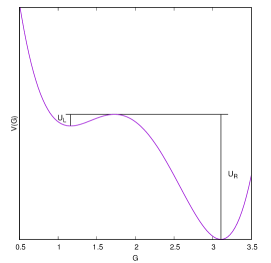
Figure 1: An asymmetric double-well potential

III An asymmetric double-well

Our first model is that of an overdamped motion in an asymmetric (tilted) double-well potential, possessing two minima, with respective depths $U_{L},U_{R}$. The particular shape of the potential is of a lesser importance, but for the purpose of this research the following potential has been used:

$$V(G)=\frac{1}{4}(G-2)^{4}-\frac{1}{2}(G-2)^{2}-\frac{1}{8}(G-2)\,,$$ (7)

where $G$ is the memductance of the system. Such a configuration may be achieved by carefully doping a semiconductor. The equation of motion is

$$\dot{G}=-\frac{dV}{dG}+V_{1}\cos{\omega t}+\sigma\,\xi(t)\,,$$ (8)

where $\xi$ is a Gaussian White Noise and $\sigma$ represents its intentsity. The amplitude $V_{1}$ is too small to drive the particle over the barrier. In this research, $V_{1}=0.2$ and $\omega=2\pi$. In the absence of the external voltage, $V_{1}=0$, the escape from a potential well forms a classic Kramers problem. Therefore, the ratio of dwelling times in the right and left potential wells is

$$\tau_{R}/\tau_{L}\sim\exp\left(\frac{U_{R}-U_{L}}{\sigma}\right).$$ (9)

The system starts in the left potential well. Without the noise, the memductance would always remain there, but thanks to the noise, it may cross the barrier and increase the current (6) transmitted by the system. Once in the right well and provided the noise is not very large, the system has a tendency to stay there and perform noisy oscillation around the deeper minimum.

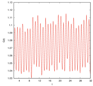
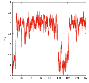
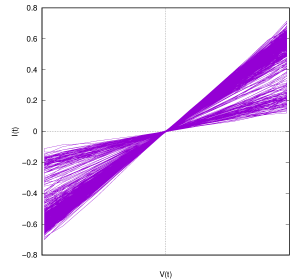
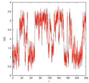
Figure 2: Example trajectories (left column) and their corresponding hysteresis loops (right column) for the system (8). Noise intensities are, top to bottom, $\sigma=0.01$, $\sigma=0.5$, and $\sigma=0.75$.

System (8) has been solved numerically with the Euler-Maruyama method and a timestep $\Delta t=1/256$. For the purpose of calculating SNR, trajectories have been averaged over 512 realizations for every single value of $\sigma$. For a very weak noise, $\sigma=0.01$, the memductance displays oscillations in the left potential well. However, consecutive minima and maxima are shifted due to the noise, and instead of a clear hysteresis loop, we can see a collection of overlapping loops. For larger noise intensities, $\sigma=0.5$, and $\sigma=0.75$ the system crosses to the right potential well and spends most of its time there. This means an increase of the memductance, but instead of a clear hysteresis loop, we obtain a combination of many overlapping, individual loops, bearing the impression of a “dirty hysteresis”, see Fig. 2. For even larger intensities of the noise, the system (8) ceases to see the fine structure of the potential and the memductance performs a random walk over all accessible range. This leads to a peculiar behavior of the SNR, see Fig. 3. For very small noises the system performs nearly perfect oscillations in the left potential well and the SNR is large. As the noise increases, it gradually destroys the oscillations and the SNR decreases, finally reaching a minimum. After that, the constructive role of noise kicks in, helping the memductance to cross to the right potential well in phase with the external voltage. The SNR reaches a maximum and a Stochastic Resonance is observed. However, for even larger values of the noise, the SNR displays a rather strange behavior: unlike in the regular SR, the SNR does not drop to zero, but reaches a plateau that extends up to unphysically large intensities of the noise.

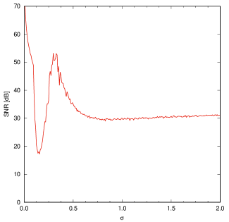
Figure 3: The Signal-To-Noise Ratio in the system (8) as a function of the GWN intensity.

This last phenomenon requires, perhaps, some attention. The power spectrum of the current (6) is related through the Wiener-Khinchin theorem to the autocorrelation $\left\langle I(t)I(t+t^{\prime})\right\rangle=\left\langle G(t)G(t+t^{\prime})\right\rangle\cos\omega t\,\cos\omega(t+t^{\prime})$. If the noise is very large, the memductance $G(t)$ discontinues to see details of the potential and is smeared over all accessible range. We may represent $G(t)$ in this regime as a random variable $\gamma(t)+\tilde{G}$, where $\left\langle\gamma(t)\right\rangle=0$, the existence of $\left\langle\gamma(t)\gamma(t+t^{\prime})\right\rangle$ is guaranteed by the fact that GWN is the driving process, and $\tilde{G}\not=0$ due to the asymmetry of the potential with respect to sign reversal. Therefore,

$$\left\langle G(t)G(t+t^{\prime})\right\rangle=\left\langle\gamma(t)\gamma(t+t^{\prime})\right\rangle+{\tilde{G}}^{2}\,.$$ (10)

The presence of ${\tilde{G}}^{2}\not=0$ is responsible for the plateau in the SNR.

Similar results, not reported here, have been obtained for a tilted triple-well potential.

IV Harmonic well with correlated noises

The other model discussed in this paper relates to the Linear Stochastic Resonance (LSR) Góra (2004). LSR is a kind of SR where signal-enhancing effect arises from cooperation between a linear transmitter and two GWNs acting on it, one multiplicative, or parametric, the other additive. Instead of (7) we take

$$V(G)=\frac{1}{2}aG^{2}-V_{0}G\,.$$ (11)

With the absence of any noises, this system leads to a time-delay behavior discussed at the beginning of the paper. We now perturb the model by two GWNs: A multiplicative, $\xi(t)$, and an additive, $\xi_{a}(t)$, noises. The evolution equation for the memductance is

$$\dot{G}(t)=-(a+p\xi(t))G+V_{0}+q\xi_{a}(t)+V_{1}\cos(\omega t+\phi)\,,$$ (12)

where $\phi$ is a random initial phase of the signal. The noises are correlated

$$\left\langle\xi(t)\xi_{a}(t^{\prime})\right\rangle=c\,\delta(t-t^{\prime})\,,\quad-1\leqslant c\leqslant 1\,.$$ (13)

We may thus represent the additive noise $\xi_{a}(t)$ as a combination of two independent GWNs

$$\xi_{a}(t)=c\,\xi(t)+\sqrt{1-c^{2}}\,\eta(t)\,,$$ (14)

with $\left\langle\xi(t)\eta(t^{\prime})\right\rangle=0$, leading to

$$\dot{G} = -(a+p\xi(t))G+V_{0}+qc\xi(t)+q\sqrt{1-c^{2}}\,\eta(t)$$ (15)

$${}+V_{1}\cos(\omega t+\phi)\,.$$

The system (15) has been discussed in Ref. Góra (2004). The formal solution with $G(0)=0$ is

$$G(t)=\int\limits_{0}^{t}e^{-a(t-t^{\prime})}\,\exp\left[-p\int\limits_{t^{\prime}}^{t}\xi(t^{\prime\prime})dt^{\prime\prime}\right]\times{}$$

$$\left(V_{0}+qc\xi(t^{\prime})+q\sqrt{1-c^{2}}\eta(t^{\prime})+V_{1}\cos(\omega t^{\prime}+\phi)\right)dt^{\prime}\,.$$ (16)

This solution has a well-defined mean if

$$a-\frac{1}{2}p^{2}>0$$ (17)

and a variance if a stronger condition

$$a-p^{2}>0$$ (18)

holds. In this case, for $V_{1}=0$, the solution is

$$\left\langle G(t)\right\rangle\mathop{\longrightarrow}\limits_{t\to\infty}G_{\infty}=\frac{V_{0}-\frac{1}{2}cpq}{a-\frac{1}{2}p^{2}}$$ (19)

and the variance asymptotically takes the form

$$\left\langle G^{2}(t)\right\rangle-\left\langle G(t)\right\rangle^{2}\mathop{\longrightarrow}\limits_{t\to\infty}$$

$$D=\frac{4V_{0}^{2}p^{2}-8aV_{0}cpq{+}(4a^{2}{-}4a(1{-}c^{2})p^{2}{+}(1{-}c^{2})p^{4})q^{2}}{2(a{-}p^{2})(p^{2}{-}2a)^{2}}\,.$$ (20)

For $V_{1}\not=0$ we can calculate the correlation function

$$\left\langle G(t)G(t+\tau)\right\rangle-\left\langle G(t)\right\rangle^{2}\mathop{\longrightarrow}\limits_{t\to\infty}\frac{V_{1}^{2}\cos(\omega\tau)}{2\left[(a-\frac{1}{2}p^{2})^{2}+\omega^{2}\right]}+\left[\frac{V_{1}^{2}p^{2}}{4(a-p^{2})\left[(a-\frac{1}{2}p^{2})^{2}+\omega^{2}\right]}+D\right]e^{-(a-\frac{1}{2}p^{2})\tau}$$ (21)

where now the braces additionally represent averaging over the initial phase of the signal.

Figure 4: Broken life — the noisy hysteresis loop for $p=0.25$, $c=1$ and with the condition (22) satisfied. The other parameters are $V_{0}=1$, $a=1$, $V_{1}=4$, $\omega=2\pi$. The colored line shows the clean hysteresis loop corresponding to the same set of parameters.

The most interesting feature of the above solution is that if

$$V_{0}p-acq=0$$ (22)

for $c\not=0$ the variance $D$ reaches a minimum. This is so because with the condition (22) satisfied, Eq. (15) can be written as

$$\dot{G} = -(a+p\xi(t))(G-V_{0}/a)+q\sqrt{1-c^{2}}\,\eta(t)$$ (23)

$${}+V_{1}\cos(\omega t+\phi)\,.$$

As we can see, part of the additive noise translates only to a shift in the equilibrium solution and $G_{\infty}=V_{0}/a$, as in the deterministic case. Furthermore, if $c=\pm 1$, the additive noise is eliminated altogether. For $D=0$ and without the external signal, $V_{1}=0$, the memristor behaves as a noise-free resistor. When $V_{1}\not=0$, $c=\pm 1$ and the condition (22) satisfied, the solution is still noisy, but minimally so for a given amplitude of the multiplicative noise, $p$, see Fig. 4.

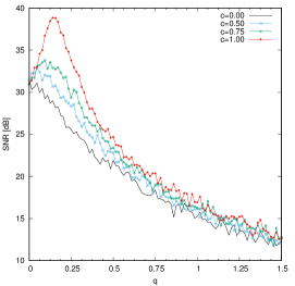
Figure 5: Numerically obtained Signal-To-Noise ratio as a function of the intensity of the additive noise, $q$, for different values of the correlation coefficient, $c$ The multiplicative noise intensity $p=0.15$. All other parameters as in Fig. 4.

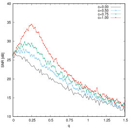
Figure 6: Same as Fig. 5, but with the multiplicative noise intensity $p=0.25$.

Because $D$ enters the expression for the correlation function (21), minimizing $D$ corresponds to optimizing the current (6) with respect to the external signal with amplitude of the multiplicative noise, $p$, fixed. We have solved Eq. (15) numerically with the Euler-Maryuama scheme with a timestep $\Delta t=1/256$. Numerical power spectra have been averaged over 128 realizations of the noises. Results for the model (15) are presented in Fig. 5. For $c=1$, a clear stochastic resonance is visible. Stochastic resonance persists for all $c\not=0$, but for small values of $c$, SR is drowned by numerical fluctuations. For uncorrelated additive and multiplicative noises, $c=0$, the stochastic resonance vanishes altogether and the resulting hysteresis loop becomes much more irregular due to the maximization of the additive noise. Trajectories representing negative memductances are clearly visible, as shown in Fig. 7.

Figure 7: Same as in Fig. 4, but for $c=0$ and $p=q=0.25$.

Interestingly, for both amplitudes of the noises, $p$ and $q$, fixed, for $c\not=0$ the resonance condition (22) can still be reached by changing $V_{0}$. This, however, means changing the shape of the noise-free hysteresis as well.

V Higher-order monostable wells

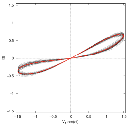
Figure 8: Broken life — the noisy hysteresis loop for the quartic well, (24) with $n=2$. $c=1$ and the condition (22) is satisfied. Parameters are $V_{0}=1$, $a=1$, $p=0.15$, $V_{1}=1.5$, $\omega=2\pi$. The colored line shows the clean hysteresis loop corresponding to the same set of parameters. (Note a different scale as compared to Fig. 4.)

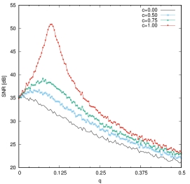
Figure 9: Numerically obtained Signal-To-Noise Ratio as a function of the intensity of the additive noise, $q$, in the model (24), for different values of the correlation coefficient, $c$. Other parameters as in Fig. 8.

Results for the LSR can be generalized to higher order monostable potential wells. Suppose that instead of relaxing in a harmonic well, the particle whose position represents the memductance relaxes in a potential $\frac{1}{2n}G^{2n}\,,n=2,3,\dots$. We now have

$$\dot{G} = -(a+p\xi(t))G^{2n-1}+V_{0}+qc\xi(t)+q\sqrt{1-c^{2}}\eta(t)$$ (24)

$${}+V_{1}\cos(\omega t+\phi)$$

and for $c\not=0$, with the condition (22) satisfied,

$$\dot{G} = -(a+p\xi(t))\left(G^{2n-1}-V_{0}/a\right)+q\sqrt{1-c^{2}}\eta(t)$$ (25)

$${}+V_{1}\cos(\omega t+\phi)\,.$$

Substituting $y=G-(V_{0}/a)^{1/(2n-1)}$ we get

$$\dot{y}=-(a+p\xi(t))yW(y)+q\sqrt{1-c^{2}}\eta(t)+V_{1}\cos(\omega t+\phi)\,,$$ (26)

where

$$W(y)=\sum\limits_{l=0}^{2(n-1)}\genfrac{(}{)}{0.0pt}{0}{2n-1}{l+1}y^{l}(V_{0}/a)^{1-\frac{l+1}{2n-1}}$$ (27)

is a polynomial of order $2(n-1)$. As we can see, correlations between the multiplicative and additive noises again result in shifting of the equilibrium solution and reducing of the additive noise. If $c=\pm 1$ and the resonance condition (22) is satisfied, the additive noise is eliminated completely.

If there is no external signal, $V_{1}=0$, and the additive noise is eliminated, Eq. (26) is formally solved as

$$\int\frac{dy}{y\,W(y)}=-at-p\int\limits_{0}^{t}\xi(t^{\prime})\,dt^{\prime}\,.$$ (28)

For $n=2$, the integral on the left-hand of Eq. (28) can be carried out analytically, but even then the resulting expression cannot be solved for $y$ explicitly. In general, Eq. (24) can be solved only numerically. Because of the nonlinear character of Eqns. (24),(26), a solution for $V_{1}\not=0$ cannot be represented as a convolution of the free solution and the external forcing, as in the linear case discussed above. However, as the integral in (28) contains a logarithmic term, we expect that the condition (18) needs to be satisfied for the variance of the solution to exist. Numerical experiments confirm this intuition.

We have solved Eq. (24) numerically for the quartic $(n=2)$ potential. The solutions display a hysteresis loop, as expected. It turns out that the nonlinearity significantly reduces the range of parameters for which negative memductances do not appear. Fig. 8 shows a hysteresis loop in a resonant case. Because with the amplitude of the multiplicative noise equal $p=0.25$ as in Fig. 4 leads to negative memductances, we have used a smaller value of $p=0.15$ and the noisy hysteresis is less blurred. Fig. 9 shows the SNR. In a quatric well stochastic resonance is even stronger than in the LSR. SR is present for all $c\not=0$, but for small values of $c$ it is hardly visible.

VI Conclusions

In this paper we have addressed the effect of noise on signal transmission in model memristive devices. On one hand side miniaturization of electronic processors allows for integration of many circuit elements per unit area and lowers the driving voltage, on the other hand, it naturally makes the systems vulnerable to thermal, $1/f$, shot and external, environmental noises. At the same time, based on theoretical approaches and experimental considerations, it has been documented that better endurance of signal transmission in natural and artificial systems can be achieved by understanding the source and making use of inherent temporal fluctuations in resistive devices. Contemporary methods used in design of artificial signal transferring systems try to mimick information processing mechanisms of living organisms and to emulate states of conductance of neuron synapses by analyzing stochastic response of neuron-like units and networks. Taken from that perspective, the Stochastic Resonance phenomenon may serve as an event optimizing performance of a system in the presence of noise, alike hearing or visual sensations have been shown to be amplified Schilling et al. (2021); Simonotto et al. (1997); Gammaitoni et al. (1998); Chialvo, Longtin, and Müller-Gerking (1997) by interference of weak signals and temporal fluctuations.

Our research shows that a conceptually very simple system of a particle relaxing in a potential well can model the memristive behavior under the influence of noise. We have discussed two kinds of models which, in addition to the memristive behavior, display a Stochastic Resonance. In the model involving a tilted double-well potential we observe a “dirty hysteresis” consisting of multiple overlapping hysteresis loops, reminiscent of hysteretic rounding observed in plastic or disordered materials. In the model involving a monostable well subject to correlated multiplicative and additive noises – a harmonic well that can be solved analytically and its generalisations to higher-order wells – a blurred hysteresis is observed, much as in the case of hysteresis loops observed in voltage-activated ion channels Gudowska-Nowak, Dybiec, and Flyvbjerg (2004); Flyvbjerg et al. (2012); Rappaport et al. (2015). This highlights a previously unexpected connection between memristive systems and ion channels. The question remains how integration of such units in neuromorphic architecture will influence properties of the circuit and its performance in signal transduction.

References

References

- Chua (1971) L. Chua, “Memristor, the missing circuit element,” IEEE Trans. Circuit Theor. 5, 507 (1971).
- Chua and Kang (1976) L. Chua and S. M. Kang, “Memristive devices and systems,” Proceedings of the IEEE 64, 209–223 (1976).
- Strukov et al. (2008) D. B. Strukov, G. S. Snider, D. R. Stewart, and R. S. Williams, “The missing memristor found,” Nature 453, 80–83 (2008).
- Pershin and Di Ventra (2011) Y. V. Pershin and M. Di Ventra, “Memory effects in complex materials and nanoscale systems,” Advances in Physics 60, 145–227 (2011).
- Chua (2014) L. Chua, “If it’s pinched it’s a memristor,” Semiconductor Science and Technology 29, 104001 (2014).
- Pershin and Di Ventra (2018) Y. Pershin and M. Di Ventra, “A simple test for ideal memristors,” Journal of Physics D: Applied Physics 52, 01LT01 (2018).
- Pershin et al. (2022) Y. V. Pershin, J. Kim, T. Datta, and M. Di Ventra, “An experimental demonstration of the memristor test,” Physica E: Low-dimensional Systems and Nanostructures 142, 115290 (2022).
- Caravelli and Carbajal (2018) F. Caravelli and J. P. Carbajal, “Memristors for the curious outsiders,” Technologies 6, 118 (2018).
- Radwan and Fouda (2015) A. G. Radwan and M. E. Fouda, On the mathematical modeling of memristor, memcapacitor and meminductor (Springer International Publishing Cham, Heidelberg, 2015).
- Battistoni et al. (2022) S. Battistoni, M. Cocuzza, S. L. Marasso, A. Verna, and V. Erokhin, “The role of the internal capacitance in organic memristive device for neuromorphic and sensing applications,” Advanced Electronic Materials 8, 2101319 (2022).
- Alonso et al. (2021) F. J. Alonso, D. Maldonado, A. M. Aguilera, and J. B. Roldán, “Memristor variability and stochastic physical properties modeling from a multivariate time series approach,” Chaos, Solitons and Fractals 143, 110461 (2021).
- Caravelli, Traversa, and Di Ventra (2017) F. Caravelli, F. L. Traversa, and M. Di Ventra, “The complex dynamics of memristive circuits: analytical results and universal slow relaxation,” Physical Review E 95, 022140 (2017).
- Roldán et al. (2023) J. B. Roldán, E. Miranda, D. Maldonado, A. N. Mikhaylov, N. V. Agudov, A. A. Dubkov, M. N. Koryazhkina, M. B. González, M. A. Villena, S. Poblador, M. Saludes-Tapia, R. Picos, F. Jiménez-Molinos, S. G. Stavrinides, E. Salvador, F. J. Alonso, F. Campabadal, B. Spagnolo, M. Lanza, and L. O. Chua, “Variability in resistive memories,” Advanced Intelligent Systems 5, 2200338 (2023).
- Wan and Shi (2022) Q. Wan and Y. Shi, Neuromorphic Devices for Brain-Inspired Computing: Artificial Intelligence, Perception and Robotics (Wiley-VCH GmbH, Hoboken, 2022).
- Hwang (2015) C. S. Hwang, “Prospective of semiconductor memory devices: from memory system to materials,” Advanced Electronic Materials 1, 1400056 (2015).
- Benzi, Sutera, and Vulpiani (1981) R. Benzi, A. Sutera, and A. Vulpiani, “The mechanism of stochastic resonance,” Journal of Physics A: Mathematical and General 14, L453 (1981).
- Nicolis and Nicolis (1981) C. Nicolis and G. Nicolis, “Stochastic aspects of climatic transitions–additive fluctuations,” Tellus 33, 225–234 (1981).
- Gammaitoni et al. (1998) L. Gammaitoni, P. Hänggi, P. Jung, and F. Marchesoni, “Stochastic resonance,” Rev. Mod. Phys. 70, 223–287 (1998).
- Bezrukov and Vodyanoy (1997) S. M. Bezrukov and I. Vodyanoy, “Stochastic resonance in non-dynamical systems without response thresholds,” Nature 385, 319–321 (1997).
- Dybiec and Gudowska-Nowak (2009) B. Dybiec and E. Gudowska-Nowak, “Lévy stable noise induced transitions: Stochastic resonance, resonant activation and dynamic hysteresis,” J. Stat. Mech.: Theory and Exp. , 05004–05020 (2009).
- Evstigneev et al. (2005) M. Evstigneev, P. Reimann, C. Schmitt, and C. Bechinger, “Quantifying stochastic resonance: theory versus experiment,” Journal of Physics: Condensed Matter 17, S3795 (2005).
- Stotland and Di Ventra (2012) A. Stotland and M. Di Ventra, “Stochastic memory: Memory enhancement due to noise,” Phys. Rev. E 85, 011116 (2012).
- Mikhaylov et al. (2021) A. Mikhaylov, D. Guseinov, A. Belov, D. Korolev, M. Shishmakova, M. Koryazhkina, D. Filatov, O. Gorshkov, D. Maldonado, F. Alonso, J. Roldán, A. Krichigin, N. Agudov, A. Dubkov, A. Carollo, and B. Spagnolo, “Stochastic resonance in a metal-oxide memristive device,” Chaos, Solitons & Fractals 144, 110723 (2021).
- Slipko and Pershin (2023) V. A. Slipko and Y. V. Pershin, “Probabilistic model of resistance jumps in memristive devices,” Phys. Rev. E 107, 064117 (2023).
- Gudowska-Nowak, Dybiec, and Flyvbjerg (2004) E. Gudowska-Nowak, B. Dybiec, and H. Flyvbjerg, “Resonant effects in a voltage-activated channel gating,” SPIE Proc. Series 5467, 223–234 (2004).
- Flyvbjerg et al. (2012) H. Flyvbjerg, E. Gudowska-Nowak, P. Christophersen, and P. Bennekou, “Modeling hysteresis observed in the human erythrocyte voltage-dependent cation channel,” Acta Phys. Pol. B 43, 2117–2140 (2012).
- Rappaport et al. (2015) S. M. Rappaport, O. Teijido, D. P. Hoogerheide, T. K. Rostovtseva, A. M. Berezhkovskii, and S. M. Bezrukov, “Conductance hysteresis in the voltage dependent anion-selective channel,” European Biophysics Journal 44, 465–472 (2015).
- Sznajd-Weron, Jedrzejewski, and Kamińska (2023) K. Sznajd-Weron, A. Jedrzejewski, and B. Kamińska, “Toward understanding of the social hysteresis: Insights from agent-based modeling,” Perspectives on Psychological Science 2023, 1–11 (2023).
- Carboni and Ielmini (2019) R. Carboni and D. Ielmini, “Stochastic memory devices for security and computing,” Advanced Electronic Materials 5, 1900198 (2019).
- Góra (2004) P. F. Góra, “The logistic equation and a linear stochastic resonance,” Acta Phys. Pol. B 35, 1583 (2004).
- Schilling et al. (2021) A. Schilling, K. Tziridis, S. H., and P. Krauss, “The stochastic resonance model of auditory perception: A unified explanation of tinnitus development, Zwicker tone illusion, and residual inhibition.” Prog Brain Res. 262, 139–157 (2021).
- Simonotto et al. (1997) E. Simonotto, M. Riani, C. Seife, M. Roberts, J. Twitty, and F. Moss, “Visual perception of stochastic resonance,” Phys. Rev. Lett. 78, 1186–1189 (1997).
- Chialvo, Longtin, and Müller-Gerking (1997) D. R. Chialvo, A. Longtin, and J. Müller-Gerking, “Stochastic resonance in models of neuronal ensembles,” Phys. Rev. E 55, 1798–1808 (1997).