MACE-OFF23: Transferable Machine Learning
Force Fields for Organic Molecules

Abstract

Classical empirical force fields have dominated biomolecular simulation for over 50 years. Although widely used in drug discovery, crystal structure prediction, and biomolecular dynamics, they generally lack the accuracy and transferability required for predictive modelling. In this paper, we introduce MACE-OFF23, a transferable force field for organic molecules created using state-of-the-art machine learning technology and first-principles reference data computed with a high level of quantum mechanical theory. MACE-OFF23 demonstrates the remarkable capabilities of local, short-range models by accurately predicting a wide variety of gas and condensed phase properties of molecular systems. It produces accurate, easy-to-converge dihedral torsion scans of unseen molecules, as well as reliable descriptions of molecular crystals and liquids, including quantum nuclear effects. We further demonstrate the capabilities of MACE-OFF23 by determining free energy surfaces in explicit solvent, as well as the folding dynamics of peptides. Finally, we simulate a fully solvated small protein, observing accurate secondary structure and vibrational spectrum. These developments enable first-principles simulations of molecular systems for the broader chemistry community at high accuracy and low computational cost.

I Introduction

Machine learning (ML) force fields have recently undergone major improvements in accuracy, robustness, and computational speed [1, 2, 3, 4, 5, 6, 7, 8, 9, 10, 11, 12, 13]. They are now routinely used in materials chemistry contexts where density functional theory was previously the method of choice. In these applications, available empirical force fields, such as the embedded-atom method [14], do not provide sufficient accuracy and transferability to describe many scientifically interesting and challenging phenomena. Successful applications of ML potentials include simulation of quenching of amorphous silicon [15], determination of the phase diagrams of inorganic perovskites [16] and alloys [17], and device-scale simulation of phase-change memory materials [18].

In contrast, simulating bio-organic systems entails a different set of trade-offs, with greater emphasis on simulating systems over long timescales. This means that empirical force fields, which sacrifice accuracy for computational speed, continue to be used routinely to study molecular liquids, crystals, biological systems, and drug-like molecules [19, 20, 21, 22].

Two alternatives to empirical force fields are available. The first is semi-empirical quantum mechanics, such as the series of extended tight-binding models [23], which represents a low-cost solution for small molecules. The method is limited by its moderate accuracy compared to quantum chemistry methods, its restriction to modelling non-periodic systems, and its cubic scaling with system size.

Secondly, a number of transferable machine learning force fields have also been developed for organic chemistry. The most notable are the series of ANI [24, 25, 26, 27] and AIMNet potentials [28, 29, 8]. ANI potentials pioneered the use of local symmetry function-based feedforward neural networks [30] trained on a large dataset of organic molecular geometries [31, 32] to create transferable force fields. The ANI-2x model became the most widely adopted ML force field and therefore serves as one of the primary points of comparison in this paper. The ANI-2x model was recently combined with a polarizable electrostatic model [33] in a hybrid ML/MM simulation setting, and also with a neural network based dispersion correction [34]. The AIMNet models apply a message passing architecture [35], where the initial embeddings are the ANI symmetry functions. They have also extended the applicability of the models to a larger set of chemical elements, as well as to charged species. These models relax the locality assumptions by incorporating electrostatic and dispersion interactions. The PhysNet model uses a message passing architecture [35] and in addition to the semi-local terms also includes long-range electrostatic and dispersion interactions [36].

Further recent bio-organic force fields include the FENNIX model, which combines a local equivariant machine learning model with a physical long-range functional form for electrostatics and dispersion [37]. The model was trained to reproduce the CCSD(T)/CBS energies of small molecules and molecular dimers. It was shown that FENNIX can be used to run stable dynamics of liquid water, solvated alanine dipeptides, and an entire protein in the gas phase. However, wider benchmarking of this model is required to assess the accuracy of the intramolecular potential outside the training set and of condensed phase molecular dynamics simulations.

Similarly, the ANA2B potential employs a short-ranged ML potential, with long-ranged, classical multipolar electrostatics, polarization and dispersion interactions [38]. Although this long-ranged model shows promising accuracy for condensed phase properties and crystal structure ranking, its accuracy and computational performance has not yet been demonstrated for larger biomolecules. Finally, the GEMS model [39], built on the SpookyNet architecture [40], is another recent ML force field for biomolecular simulations. Although SpookyNet has demonstrated application to more challenging condensed phase simulations, including protein dynamics, these required a significant number of reference quantum chemistry calculations on relevant large peptide fragments for each new simulation to obtain a stable model and is therefore not transferable in the sense that the previously discussed force fields are.

In this paper, we introduce a series of three purely local transferable bio-organic machine learning force fields called MACE-OFF23. The force fields are parameterized for the ten most important chemical elements for organic chemistry H, C, N, O, F, P, S, Cl, Br, and I. They are capable of accurately describing intra- and intermolecular interactions of neutral closed-shell systems. This enables the simulation of a wide range of chemical systems, from molecular liquids and crystals to drug-like molecules and biopolymers.

The models were validated on a number of tasks, including the prediction of small molecule torsion barriers, geometry optimizations, calculations of lattice parameters and enthalpies of formation of molecular crystals, and the calculation of the Raman spectra of molecular crystals, including nuclear quantum effects. We have also validated the models for predicting the densities and heats of vaporization of a range of molecular liquids. In particular, we study how well MACE-OFF23 reproduces the basic properties of water, including density and radial distribution functions. To further showcase the capabilities of the model, we computed the free energy surface of the alanine tripeptide (Ala₃) in vacuum and explicit water, and simulated the folding of Ala₁₅ at different temperatures. We also carried out an all-atom simulation of the protein crambin in explicit water (18 000 atoms), where we observed the expected secondary structure and computed its vibrational spectrum finding good agreement with previously reported experimental data. Finally, we tested the computational speed of the current implementation in the LAMMPS and OpenMM simulation packages.

II Methods

II.1 The MACE architecture

The MACE model [2] is a force field that maps the positions and chemical elements of atoms to the system’s potential energy. Linear scaling with system size is achieved by decomposing the total energy into atomic site energies. First, a graph is defined by connecting two nodes (atoms) by an edge if they are in each other’s local environment. The local environment $\mathcal{N}(i)$ is the set of all atoms $j$ around the central atom $i$ for which $\|\bm{r}_{ij}\|\leq r_{\text{cut}}$, where $\bm{r}_{ij}$ is the vector from atom $i$ to atom $j$ and $r_{\text{cut}}$ is the cutoff hyperparameter. The array of features of node $i$ is denoted by ${\bm{h}}_{i}^{(t)}$ and is expressed in the spherical harmonic basis, with its elements indexed by $l$ and $m$. The superscript in $t$ indicates the iteration steps (corresponding to “layers” of message passing in the language of graph neural networks). All MACE-OFF23 models are made up of two layers. The ${\bm{h}}^{(t)}_{i}$ features depend on the chemical environment of the atoms.

The node features ${\bm{h}}^{(0)}_{i}$ are initialized as a (learnable) embedding of the chemical elements with atomic numbers $z_{i}$ into $k$ channels:

$$h_{i,k00}^{(0)}=\sum_{z}W_{kz}\delta_{zz_{i}}$$ (1)

The superscript $(0)$ in this case indicates the initial (0-th) layer. This type of mapping has been widely applied to graph neural networks [41, 42, 43] and other models [44, 45].

Next, for each atom, the features of its neighbours are combined with the interatomic displacement vectors, $\bm{r}_{ij}$, to form the one-particle basis $\phi_{ij,k\eta_{1}l_{3}m_{3}}^{(t)}$. The radial distance is used as an input into a learnable radial function $R(r_{ij})$ with several outputs that correspond to the different ways in which the displacement vector and the node features can be combined while preserving equivariance [46]:

$$\phi_{ij,k\eta_{1}l_{3}m_{3}}^{(t)} =\sum_{l_{1}l_{2}m_{1}m_{2}}C_{\eta_{1},l_{1}m_{1}l_{2}m_{2}}^{l_{3}m_{3}}R_{k\eta_{1}l_{1}l_{2}l_{3}}^{(t)}(r_{ij})\,\,\times$$

$$\qquad\qquad\times Y^{m_{1}}_{l_{1}}(\bm{\hat{r}}_{ij})h^{(t)}_{j,kl_{2}m_{2}}$$ (2)

where $Y_{l}^{m}$ are the spherical harmonics, and $C_{\eta_{1},l_{1}m_{1}l_{2}m_{2}}^{l_{3}m_{3}}$ denotes the Clebsch-Gordan coefficients. There are multiple ways of constructing an equivariant combination with a given symmetry $(l_{3},m_{3})$, and these multiplicities are enumerated by the path index $\eta_{1}$ [47, 2].

The one-particle basis $\phi$ is summed over the neighborhood and expanded in a linear combination of $k$ channels with learnable weights to form the permutation invariant atomic basis $A_{i}$:

$$A_{i,kl_{3}m_{3}}^{(t)}=\sum_{\tilde{k},\eta_{1}}W_{k\tilde{k}\eta_{1}l_{3}}^{(t)}\sum_{j\in\mathcal{N}(i)}\phi_{ij,\tilde{k}\eta_{1}l_{3}m_{3}}^{(t)}$$ (3)

Higher-order (many-body) symmetric features are created on each atom by taking products of the atomic basis, $A$, with itself $\nu$ times, resulting in the “product basis”. The product basis is then contracted with the generalised Clebsch-Gordan coefficients $\mathcal{C}^{LM}_{\eta_{\nu}\bm{l}\bm{m}}$ to obtain the equivariant higher-order basis, $\bm{B}_{i}$ [47, 2]. The maximum body-order is controlled by the parameter $\nu$ and is fixed at 3 (corresponding to 4-body terms, which includes the central atom) for all MACE-OFF23 models:

$${\bm{B}}^{(t),\nu}_{i,\eta_{\nu}kLM}=\sum_{{\bm{l}}{\bm{m}}}\mathcal{C}^{LM}_{\eta_{\nu}\bm{l}\bm{m}}\prod_{\xi=1}^{\nu}A_{i,kl_{\xi}m_{\xi}}^{(t)}$$ (4)

where bold $\bm{l}\bm{m}$ denostes the $\nu$-tuple of $l$ and $m$ values and similarly to Equation (II.1), $\eta_{\nu}$ enumerates the number of possible couplings to create the features with equivariance $LM$.

Finally, a “message” $m_{i}$ is created on each atom as a learnable linear combination of the equivariant many-body features:

$$m_{i,kLM}^{(t)}=\sum_{\nu}\sum_{\eta_{\nu}}W_{z_{i}\eta_{\nu}kL}^{(t),\nu}{\bm{B}}^{(t),\nu}_{i,\eta_{\nu}kLM}$$ (5)

The recursive update of the node features ($t:0\rightarrow 2$) is obtained by adding the message to the atoms’ features from the previous iteration, with weights that depend on the chemical element ($z_{i}$) that are also responsible for the mixing of the chemical embedding $k$ channels:

$$h^{(t+1)}_{i,kLM}=\sum_{\tilde{k}}W_{kL,\tilde{k}}^{(t)}m_{i,\tilde{k}LM}^{(t)}+\sum_{\tilde{k}}W_{kz_{i}L,\tilde{k}}^{(t)}h^{(t)}_{i,\tilde{k}LM}$$ (6)

Since the initial node features ${\bm{h}}^{(0)}$ are only dependent on the chemical element of the node, the second term of Eq. (6) is not included in the first layer. This makes it possible to set the energy of the isolated atoms (that is, those with no neighbours) exactly [48], which is often desirable [49, 37].

The MACE models in this article have an effective receptive field of $2\times r_{\text{cut}}$ due to the two message-passing layers used in each model.

The site energy is a sum of read-out functions applied to node features from the first and second layers. The read-out function is defined as a linear combination of rotationally invariant node features for the first layer, and as multi-layer perceptron (MLP) for the second layer.

$$E_{i}=\sum_{t=1}^{2}E_{i}^{(t)}=\sum_{t=1}^{2}\mathcal{R}^{(t)}\left({\bm{h}}_{i}^{(t)}\right),$$ (7)

$$\mathcal{R}^{(t)}\left(\bm{h}_{i}^{(t)}\right)=\begin{cases}\sum_{k}W^{(t)}_{k}h^{(t)}_{i,k00}&\text{for}\;\;t=1\\[13.0pt] {\rm MLP}\left(\left\{h^{(t)}_{i,k00}\right\}_{k}\right)&\text{for}\;\;t=2\end{cases}$$ (8)

The forces and stresses on the atoms are calculated by taking analytical derivatives of the total potential energy with respect to the positions of the atoms.

II.2 Training data

The core of the training set is the SPICE dataset [50]. 95% of the data were used for training and validation, and 5% for testing. Table 1 summarizes the training and test sets. The MACE-OFF23 model is trained to reproduce the energies and forces computed at the B97M-D3(BJ)/def2-TZVPPD level of quantum mechanics [51, 52, 53, 54, 55], as implemented in the PSI4 software [56]. We have used a subset of SPICE that contains the ten chemical elements H, C, N, O, F, P, S, Cl, Br, and I, and has a neutral formal charge. We have also removed the ion pairs subset. Overall, we used about 85% of the full SPICE dataset. The geometries in the SPICE dataset have been generated by running molecular dynamics simulations using classical force fields [57] and sampling maximally different conformations from the trajectories [50].

Table 1: Summary of training and test sets The columns PubChem to Solvated Amino Acids correspond to the SPICE dataset [50].

	PubChem	DES370K Monomers	DES370K Dimers [58]	Dipeptides	Solvated Amino Acids	Water	QMugs [59]	Tripeptides
Chemical elements	H, C, N, O, F, P, S, Cl, Br, I	H, C, N, O, F, P, S, Cl, Br, I	H, C, N, O, F, P, S, Cl, Br, I	H, C, N, O, S	H, C, N, O, S	H, O	H, C, N, O, F, P, S, Cl, Br, I	H, C, N, O
System size	3-50	3-22	4-34	26-60	79-96	3-150	51-90	30-69
# Train	646821	16861	263065	19773	948	1597	2748	0
# Test	33884	889	13896	1025	52	84	144	898

The SPICE dataset only contains small molecules of up to 50 atoms. To facilitate the learning of intramolecular non-bonded interactions, we augmented SPICE with larger 50–90 atom molecules randomly selected from the QMugs dataset [59]. The geometries were generated by running molecular dynamics simulations using GFN2-xTB [23] similarly to the protocol described in Ref. [60]. The energies and forces were re-evaluated at the level of QM theory used in SPICE. Finally, to obtain a better description of water, the dataset was further augmented with a number of water clusters carved out of molecular dynamics simulations of liquid water [61], with sizes of up to 50 water molecules.

In addition to the 5% of each subset, part of the COMP6 tripeptide geometry dataset [25] was also recomputed at the SPICE level of theory and used as part of the test evaluation, but not for training.

After training the small MACE model (see Section II.3) and observing the training errors, we noticed the presence of outliers in the dataset. This is probably caused by errors in the underlying electronic structure calculations, some of which have been documented on the SPICE GitHub repository. To confirm this, we also re-evaluated a selection of the configurations that had the highest error, using the level of DFT used in SPICE, and found that for about a third of the configurations, the recomputed energies and forces agreed well with the MACE prediction and not with the original DFT labels. To purify the dataset, we removed from the training set the configurations that had a maximum force error greater than 2 eV/Å. This meant the removal of just 808 configurations, many of which contained heavy elements, in particular phosphorus and iodine, that might have a more challenging electronic structure.

II.3 Training details

The MACE model has parameters that enable systematic control of model expressivity (accuracy) against computational cost. In this paper, we present three variants of the MACE-OFF23 model, a small, a medium, and a large one, denoted in the text as MACE-OFF23(S), MACE-OFF23(M) and MACE-OFF23(L) respectively. The models get more accurate with size, but also have an increasing computational cost. The small model is well suited for large-scale simulations, the medium model offers a good balance of speed and accuracy, and the large model is best used for small systems or when the highest possible accuracy is desirable.

Table 2: Hyperparameters of the three MACE-OFF23 models

	Small	Medium	Large
Cutoff radius (Å)	4.5	5.0	5.0
Chemical channels	96	128	192
$k$ (Eq. (1))
max L (Eq. (5))	0	1	2

The hyperparameters of the models are displayed in Table 2. The MACE-OFF23(S) model has 96 channels, $L=0$ invariant messages, and a cutoff of 4.5 Å. The MACE-OFF23(M) model has 128 channels and $L=1$ messages, and finally the MACE-OFF23(L) has 192 channels and $L=2$ equivariant messages. Medium and large models have a cutoff of 5.0 Å in each layer. All models used two layers and a body order of 4 in each layer. The models were trained using the PyTorch [62] implementation of MACE, available on https://github.com/ACEsuit/mace. For more information about the training, please refer to the SI.

III Results

III.1 Extended SPICE Test Set

First, we look at the pointwise errors of the energy and force predictions on a held-out test set for each of the three MACE-OFF models. Figure 1 shows the per-atom energy, force and intermolecular force root-mean-square errors (full statistics are provided in SI Table 3). As the size of the model increases, the models gradually become more accurate, with the large model generally achieving errors of around 0.5–1.0 meV/atom and 15–20 meV/Å, well below the 1 kcal/mol (43 meV) chemical accuracy limit for the drug-like organic molecules studied here.

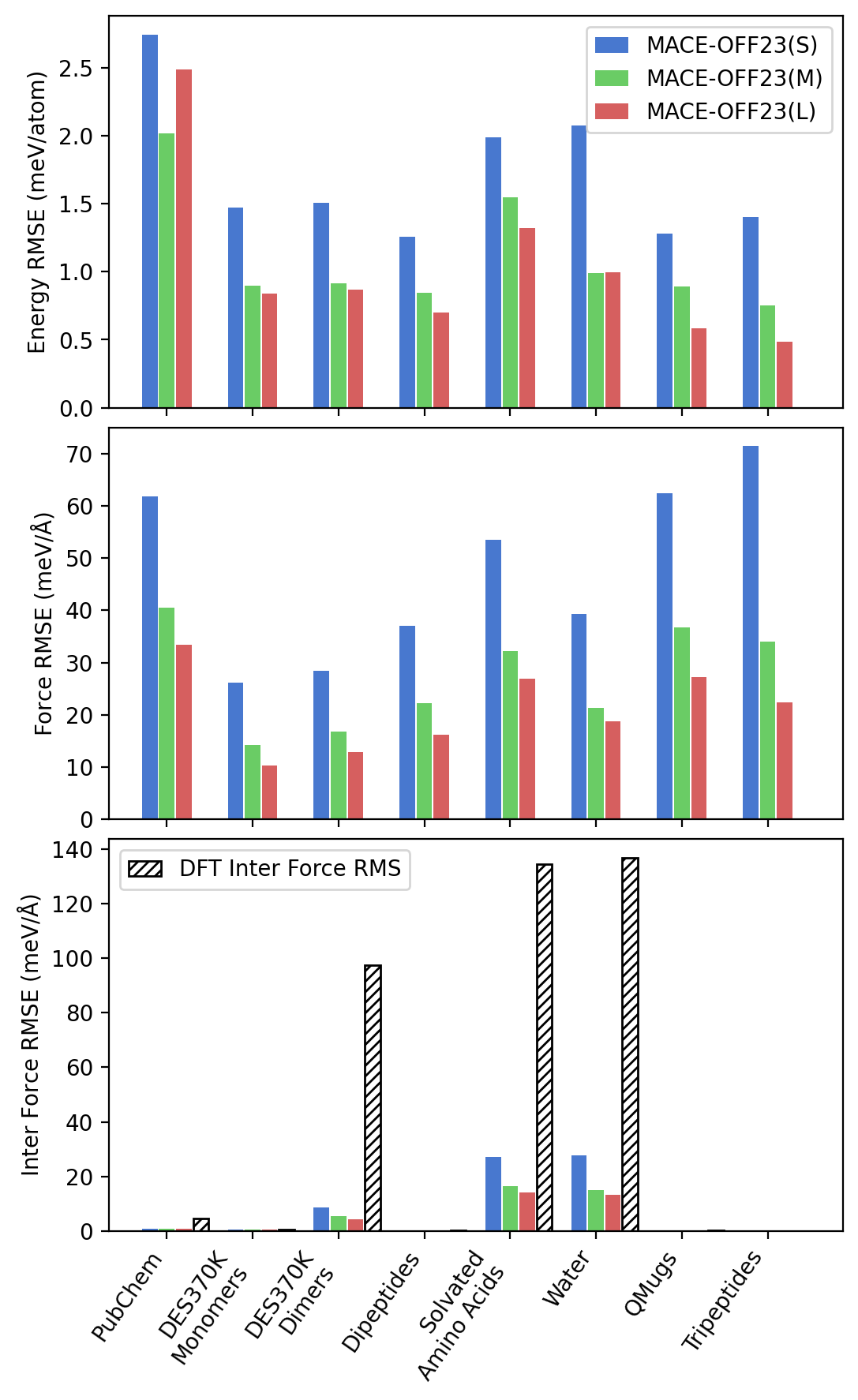
Figure 1: Test set root mean square errors (RMSE). Errors in the MACE-OFF23 models compared to the underlying DFT reference data, highlighting the relative accuracy of the three models. Bottom panels show specifically inter-molecular force errors compared to overall DFT inter-molecular force magnitudes (RMS).

The last column looks at an extrapolation task, the training set contains only dipeptides, and this test set looks at tripeptides, indicating that the models are able to extrapolate to larger fragments with more complex interactions, with no degradation of accuracy.

The bottom panel of Figure 1 shows specifically the intermolecular force errors, which were obtained by separating the force contributions to molecular translations and rotations (see SI and Ref. [63] for details). These interactions are crucially important as they underpin the thermodynamics and transport properties in the organic condensed phase. MACE medium and large models yield similar errors of around 5–15 meV/Å, which are about 1.5–3 times smaller than total force errors, and about 5–10% of the typical DFT intermolecular force magnitude (RMS). For context, relative intramolecular force errors, which are roughly equivalent to total force errors, are around 1–2%. The latter are routinely used across the literature to benchmark ML models, however, we advocate that intermolecular RMSE errors are a more appropriate metric to assess model accuracy for organic condensed phase applications. The results here demonstrate the remarkable accuracy of MACE models in predicting these subtle but crucial interactions.

III.2 Dihedral scans

Next, we evaluate the performance of the MACE-OFF23 models on dihedral scans of drug-like molecules. This task is routinely carried out using quantum mechanical methods to create reference data for parameterizing classical empirical force field dihedral terms [64]. The task is particularly challenging, as constrained geometry optimisations can be difficult to converge if the potential energy surface is not smooth, as has been observed in particular for the ANI family of potentials [65].

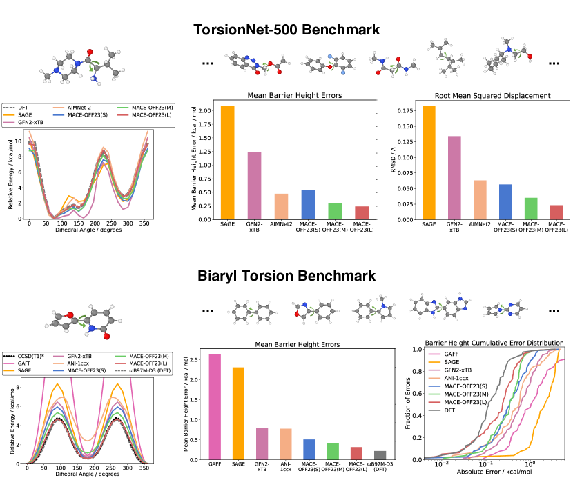
Figure 2: Dihedral benchmark scans. The top panel shows torsion drive data for the TorsionNet-500 dataset, which has a wide chemical diversity (five example molecules are shown). The bottom panel focuses on the torsion angle between two aromatic rings in the biaryl torsion benchmark [66] which contains 78 molecules (five examples are shown).

III.2.1 TorsionNet-500

The top panel of Figure 2 summarises the results for the TorsionNet-500 dataset [67]. This dataset contains torsion drives of 500 different molecules, selected to cover a wide range of pharmaceutically relevant chemical space. The original data set was reported at the B3LYP/6-31G(d) level of DFT theory. For consistency with the SPICE dataset, we recreated the torsion profiles using the DFT setting of SPICE, which is a higher level of theory (SI Section C).

The first panel shows an example of a torsion drive, indicating the complex energy profile that the MACE models are able to capture closely, including geometries far from equilibrium. The centre panel shows the mean barrier height error of a number of representative models, comparing the Sage classical empirical force field [21], a semi-empirical quantum mechanical method GFN2-xTB [23], a recent transferable machine learning force field AIMNet-2 [8], and the three MACE-OFF23 models. Again, systematic improvements in accuracy with MACE model size are observed, with medium and large models, in particular, achieving errors of around 0.25 kcal/mol compared to the reference method. The AIMNet-2 model achieves comparable accuracy to the small MACE-OFF23 model. A similar conclusion can be drawn from the comparison of the molecular geometries by looking at the root mean squared deviation of the atomic positions averaged over the full torsion scans, as indicated by the top right panel of Figure 2. It shows that MACE-optimised geometries have a deviation of about 0.025 Å, meaning they are almost indistinguishable from DFT-optimised structures. It is important to note that the different models were trained to different levels of DFT, which might also contribute to the observed differences.

III.2.2 Biaryl fragments

The biaryl torsion benchmark investigates the torsional profiles of about 100 different biaryl fragments computed at the coupled cluster level of theory [66]. In these molecules, the rotatable bond is between two aromatic rings. Such chemistry frequently occurs in drug-like molecules, and the profiles are typically challenging to model accurately using empirical classical force fields. Following previous studies, we used a subset of 78 molecules to facilitate comparisons with the ANI-1ccx model, which is only parameterized for H, C, N, and O chemical elements [66].

In the bottom panel of Figure 2, we compare the results of torsion drives of empirical force fields, semi-empirical QM methods, and the ANI-1ccx machine learning force field [26] with the MACE-OFF23 models. We also compare the DFT potential energy surfaces (using the SPICE level of theory) with the published gold standard coupled cluster data.

The DFT torsion drives achieve a mean barrier height error of 0.2 kcal/mol with respect to coupled cluster data, and is therefore the best result theoretically possible for MACE-OFF23 models which were trained on the same DFT level of theory. We find that the large model comes close to this, with a mean absolute error of 0.3 kcal/mol. The medium and small MACE models have barrier height errors of 0.4 and 0.5 kcal/mol, respectively. Remarkably, the small MACE model is significantly more accurate than the next-best non-DFT methods, ANI-1ccx and GFN2-xTB, as illustrated in the bottom-center plot of Figure 2. In particular, unlike MACE-OFF23, coupled cluster reference calculations were used to parameterize the ANI-1ccx and GFN2 models. In the bottom right, we also show the cumulative error distributions to verify that the MACE-OFF23 barrier height errors are not only accurate on average but are also robust, having essentially no outliers.

III.3 Molecular crystals

In the following, we demonstrate the ability of the MACE-OFF23 force fields to simulate the vibrational and thermal properties of molecular crystals.

III.3.1 Vibrational spectroscopy of paracetamol

Raman spectroscopy is one of the most widely used techniques for characterizing molecular crystals. Unlike IR spectroscopy, which only detects vibrational modes that distort dipoles, Raman spectroscopy is more sensitive to collective modes governed by weak, non-bonded interactions in a broad range of molecular materials. The low-frequency region of the Raman spectrum (e.g., the THz regime) gives a vibrational fingerprint of the intermolecular interactions. Thus, it is widely used to differentiate between polymorphs of molecular crystals. Meanwhile, the high-frequency Raman spectrum probes intramolecular modes and their coupling to low-frequency modes.

Here, we test the ability of the MACE-OFF23(S) model to predict the Raman spectrum of the “Form II” polymorph of paracetamol. To compare MACE-OFF23(S) directly with experiments, we rigorously incorporate quantum nuclear and non-Condon effects using our ML-aided framework [68]. We incorporate quantum nuclear effects by fitting an effective potential energy surface [69] (using MACE) to calculate quantum nuclear corrections to the MACE-OFF23(S) model within the path-integral coarse-grained simulations (PIGS) method. To incorporate non-Condon effects, we fit a separate equivariant MACE model to the first-principles polarizability of paracetamol polymorphs (data taken from Refs. 70, 71). The remaining steps of our quantum nuclear simulations mimic an entirely classical calculation involving a $NVE$ molecular dynamics simulation, prediction of the isotropic and anisotropic components of the polarizability tensor, and calculation of their time correlation functions. For further details we refer the reader to Ref. 68.

As shown in Figure 3, we predict both the high- and low-frequency regions of the Raman spectrum of paracetamol form II with an overall good agreement with the experimental band positions [72]. Since the experiment captures the Raman spectra along different crystal directions while we estimate the “powder” Raman spectrum [71], we do not compare band intensities. We find that the classical predictions (based on MACE classical MD) are consistently shifted with respect to the experiment. At the same time, quantum nuclear predictions (encoded by the PIGS method) play an essential role in improving the agreement between theory and experiments. Moreover, we note that a broad band at around 3300 $\text{cm}^{-1}$ is only captured at the level incorporating quantum nuclear effects. The low-frequency modes also agree semi-quantitatively with the experiments and do not require a quantum nuclear description. The 2–3 % overall shift in the vibrational frequencies notwithstanding, the MACE-OFF23(S) combined with quantum nuclear effects and non-Condon effects shows promising capabilities for the characterization of molecular crystals.

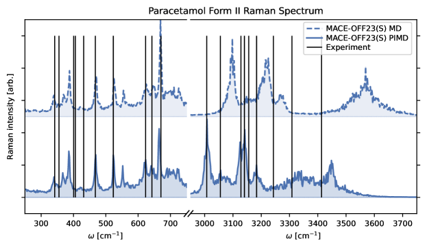
Figure 3: Powder Raman spectrum of paracetamol form II [73]. Spectrum computed at ambient conditions using the MACE-OFF23(S) model for the potential energy surface, a MACE model of the polarizability, and a MACE model that incorporates quantum nuclear effects on the potential energy surface using the PIGS approach [69]. The black lines represent experimentally determined band positions [72], scaled by 3% to aid visual comparison with the predicted spectra.

III.3.2 Lattice enthalphies

Next, we assess the ability of the MACE-OFF23 force fields to describe the stability of molecular crystals. We computed the enthalpies of sublimation of a range of 23 representative small molecular crystals [74] following the protocol of Ref. [75].

Figure 4 compares the predicted sublimation enthalpies with the experimentally measured ones. This task is often used to test various DFT functionals. Since the B97M-D3(BJ) functional used to parameterize MACE-OFF23 does not have a periodic implementation, an estimate of the highest achievable accuracy is not available. The figure shows that the three MACE models are able to capture trends and improve significantly compared to the ANI-2x model. The large MACE-OFF23 model achieves a mean error of just 1.7 kcal/mol, which is comparable to the errors of several different dispersion-corrected density functionals for a fraction of the computational cost [74].

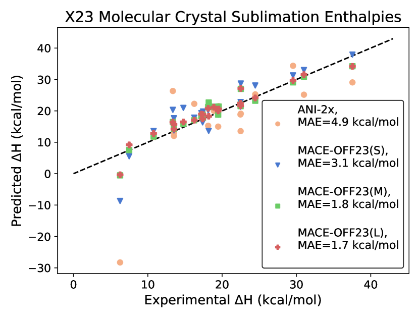
Figure 4: Sublimation enthalphies of molecular crystals. Comparison between predicted sublimation enthalphies of the MACE and ANI models and experiment.

We have also compared the relaxed unit cell vectors of the MACE-OFF23 models with the experimentally measured values and found that they have a relative error as low as 5% with the MACE-OFF23(L) model as shown in the supporting Table 8.

III.4 Water structure and dynamics

A key requirement for bio-organic force fields is a good description of water. Several empirical water models have been developed for this purpose, the most common for all-atom biomolecular simulations being TIP3P. Figure 5 shows that both MACE-OFF23(S) and MACE-OFF23(M) correctly predict the radial distribution function (RDF) of water, performing comparably with both TIP3P and the highly accurate MB-pol water model [76]. These interactions are modelled in a purely local way by MACE, having been trained on small water clusters containing up to 50 water molecules. This result further emphasizes the ability of the model to generalize to bulk simulations, even though the training data only contained non-periodic clusters. In contrast, ANI-2X shows a significant over-structuring of the RDF, likely due to the lack of dispersion correction in the underlying quantum mechanical method used to label the training set.

We further calculated the temperature dependence of the density using NPT molecular dynamics simulations, as shown in Supplementary Figure 11. This is a highly sensitive test for the accuracy of intermolecular interactions [63]. Both the small and medium models over-predict the density to a small extent, which likely originates from the underlying DFT functional or the lack of periodic training data.

Next, we characterize the dynamical properties of water by computing the vibrational density of states, including the IR and Raman spectra selection rules, using MACE models of dipoles and polarizabilities [68]. Given the significant impact of quantum nuclear motion on the dynamics of water [69], we incorporate quantum nuclear effects using the PIGS approach [69] (discussed in Section III.3.1), which has a classical cost and has recently been shown to describe quantum nuclear effects in water accurately [77]. As shown in Figure 5, after incorporating quantum nuclear effects, the MACE-OFF23(S) predictions agree with the experiments across the entire frequency range. We note the presence of an overall 2-3 % blue shift with respect to the experiments, consistent with the spectra for paracetamol form II (see Section III.3.1). MACE-OFF23(S) even qualitatively captures subtle features of the spectra, including the 0 – 1000 $\text{cm}^{-1}$ hydrogen bonding fingerprints in the anisotropic Raman spectrum, and the bimodal nature of the isotropic Raman stretching band arising from the presence of hydrogen-bonded defects in room temperature water.

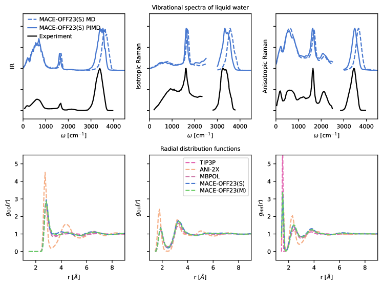
Figure 5: Water structure and dynamics. Top: IR, isotropic Raman and anisotropic Raman spectra of water at ambient temperature and density using the MACE-OFF23(S) model for the potential energy surface and a single MACE model of water’s dipole and polarizability [68]. The black curve represents the experiment [78]. The dashed blue curve is obtained from standard (classical) MD, while the solid curve incorporates quantum effects using the PIGS method [69]. Bottom: Radial distribution function of MACE, ANI and TIP3P models. MB-pol traces are reproduced from Ref. [76]

.

III.5 Condensed phase properties of organic liquids

Small molecule empirical force fields are fitted to reproduce experimental condensed phase properties including densities and heats of vaporization. For machine learning force fields, this task represents a greater challenge, since the potential is typically trained only using QM reference data for isolated molecules and molecular dimers. From these ab initio data, the models infer the long-range interactions necessary to reproduce bulk properties without ever fitting to them.

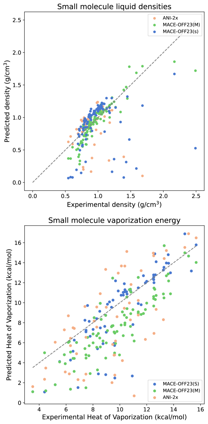
Figure 6: Molecular liquids. Comparison between MACE-OFF23(M) and ANI-2x with experiment for densities (top) and heats of vaporization (bottom) of condensed phase organic liquids.

To investigate the performance of the MACE-OFF23 models in the condensed phase, we selected a benchmark set of 109 molecules from Ref. [79], containing a representative set of functional groups relevant to medicinal chemistry and biology. The medium MACE-OFF23 model has a larger receptive field and is therefore better suited for reproducing experimental observables most affected by intermolecular interactions. In general, we found that the small model gave a reasonable description in the NVT ensemble, while the medium model is also able to accurately model liquids in NPT simulations, as detailed below. For the liquid boxes containing approx. 1000 atoms, MACE-OFF23(S) achieved a throughput of $2.1\pm 1.2\mathrm{x}10^{6}$ steps/day, whilst the medium model achieved a throughput of $1.4\pm 1.1\mathrm{x}10^{6}$ steps/day.

First, we investigate the predictions of molecular liquid densities under ambient conditions using the medium MACE model shown on the top panel of Figure 6. The MACE-OFF23(M) model achieves a MAE of 0.09 g/cm³, indicating that it can generalize from the intermolecular interactions between molecular dimers in the training set to the condensed phase, retaining a good correlation with experiment. In contrast, the ANI-2x potential has significantly higher errors, with MAE and RMSE errors twice as large as MACE-OFF23(M).

Most of the outliers predicted by MACE-OFF23(M) sit at the extreme ends of the spectrum. We found that the densities of low boiling point ether-containing compounds were under-predicted, likely because they begin to boil off at the simulation temperature, since the potential marginally under-predicts their boiling points. At the top end of the density range, the dibromo compounds were also under-predicted. This is perhaps unsurprising since there are only 84 configurations in the training set containing dimers of dibromo compounds.

Interestingly, we found that MACE-OFF23(S) systematically overpredicts the experimental densities (SI Table 4) with a MAE of 0.23 g/cm³. This is likely the result of the slightly higher energy error and the shorter cutoff radius. In particular, the contribution of the intermolecular interactions to the overall energy is much smaller than the intramolecular interactions making the fractional error in them much larger. This is demonstrated in SI Table 3, where the test errors are decomposed into inter- and intramolecular contributions. We find that the medium and large models have significantly lower intermolecular force errors.

We further investigate the performance of MACE-OFF23(M) on heats of vaporization. The predictions correlate strongly with the experimental data ($r^{2}$=0.88), however there is a systematic offset of approximately 2 kcal/mol. This may result from an under-prediction of the total intermolecular interactions originating from two sources: those that appear in molecular dynamics simulations outside the effective cutoff of the MACE model (c.f. classical simulations, which typically employ long-range corrections to the total energy [80]), and those that the model has not learned from the limited set of intermolecular interactions in the training set.

Interestingly, for MACE-OFF23(S), this offset disappears (see SI Table 5), however this is likely due to the unphysically high predicted densities, resulting in a cancellation of errors through overprediction of the magnitude of intermolecular interactions. Nevertheless, these data indicate that, given a reasonable receptive field and a sufficiently expressive model, it is possible to fit a local force field that captures the interactions required to recover experimental properties.

III.6 Peptide Simulations

In the following section, we benchmark the performance of MACE-OFF23(S) on several well-studied large-scale biomolecular systems. We selected the small model since it is capable of accurately reproducing the properties of bulk water (Section III.4), while also having the computational speed required to simulate large systems over long timescales. This particular application area is of key interest, and state-of-the-art classical protein force fields have been carefully parameterized over many decades to reproduce key quantum mechanical and thermodynamic properties. However, this extensive parameterization process makes it difficult to extend classical force fields, and overall accuracy and transferability remain fundamentally limited by their functional form, which typically becomes apparent only when each generation of advancing hardware enables sufficiently long simulations to identify issues.

III.6.1 Ala₃ Free Energy Surface

We first studied the ability of MACE to reproduce the free energy surface of the Ala₃ tripeptide. Using the MACE-OFF23(S) force field, we observed computational performance of 7.5 ns/day for the vacuum system, and 2.2 ns/day for the solvated system, using a 1 fs timestep. Although this remains significantly more expensive than the MM simulation (around 300 ns/day with a 2 fs timestep), it nevertheless enables sufficient sampling of the potential energy surface in a reasonable compute time.

Figure 7 shows the free energy surface of Ala₃ in water, modelled by AMBER14/TIP3P and MACE, respectively, sampled along the central $\phi$ and $\psi$ backbone angles. The AMBER14 simulations identify several local minima, corresponding to the anti-parallel $\beta$-sheet ($\phi<-120^{\circ},\psi>120^{\circ}$), a right-handed $\alpha$-helix ($\phi=-60^{\circ},\psi>-60^{\circ}$), the corresponding left-handed $\alpha$-helix ($\phi=60^{\circ},\psi>60^{\circ}$), and a polyproline II (PPII)-type structure ($\phi=-60^{\circ},\psi>120^{\circ}$). Compared to experimental fits of the NMR J-coupling constants [81], the AMBER14 simulation is generally in good agreement, with a slight overpopulation of both $\alpha$-helical structures and underpopulation of the PPII mesostate.

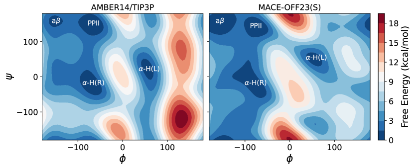
Figure 7: Free energy surfaces of Ala₃ in explicit solvent. Free energies have been normalized to zero at the minimum to aid visual comparison.

The corresponding MACE simulations show a very similar free energy surface to AMBER14/TIP3P, with the same four local minima identified. Whilst the relative depths of the -helical conformations are in agreement, AMBER predicts the free energy of the anti-parallel -sheet to be 1 kcal/mol higher than the PPII minimum, compared to 0.1 kcal/mol for MACE.

III.6.2 Folding dynamics of Ala₁₅

Having confirmed that MACE is capable of constructing the free energy surface of a small peptide, we next investigated the folding of the longer helical peptide Ala₁₅. Since this is a significantly larger system size than the dipeptide configurations that the model was trained on, this represents a nontrivial test of the extrapolation capability of the potential, including its ability to capture complex hydrogen bonding patterns required to stabilize the secondary structure. Such simulations are believed to be particularly difficult with purely local models such as MACE-OFF23.

As an initial test, the fully extended Ala₁₅ structure was prepared and simulated in vacuo with MACE-OFF23(S). The top right panel of Figure 8 shows the assignment of the secondary structure during the simulation. The peptide rapidly folded into a stable helical structure, which was confirmed using hydrogen bonding counts.

We also measured the secondary structure of the peptide during trajectories collected at three higher temperatures. This analysis confirmed that the helical secondary structure is stable up to around 700 K, while at 800 K the hydrogen bond count significantly decreases, consistent with the experimental unfolding temperature of 725 K as shown in the two bottom panels of Figure 8.

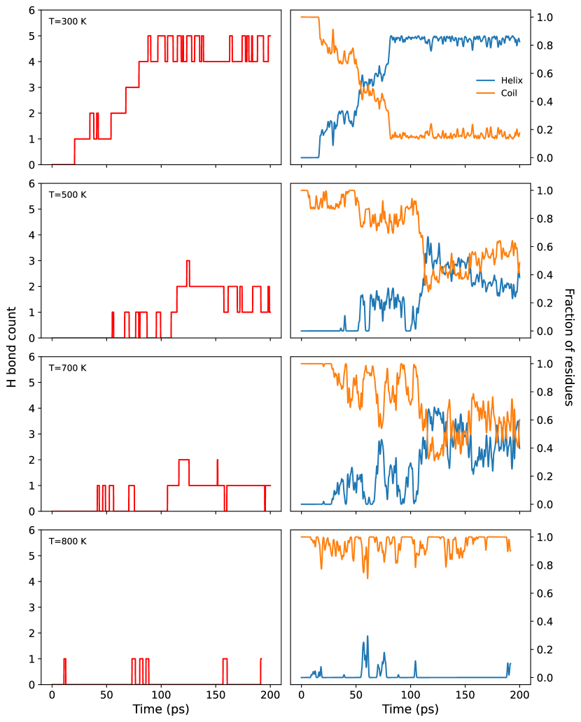
Figure 8: Ala₁₅ folding dynamics. Left: Hydrogen bond count using the DSSP algorithm [82] along the Ala₁₅ trajectory at four different temperatures. Right: Secondary structure of Ala₁₅ during the folding trajectory.

III.6.3 Protein simulation in explicit solvent

Finally, we investigated the simulation of a fully solvated protein with MACE-OFF23. As a test case, we chose crambin, a 42 residue threonin storage protein containing four charged residues. This test goes well beyond what can typically be expected from a short-ranged force field trained on neutral species only.

Using the MACE-OFF23(S) model, we first confirmed that the force field was indeed capable of simulating a large biomolecular system containing charged residues. In particular, it has recently been shown that the FENNIX potential fails to simulate a solvated 28 residue peptide due to unphysical proton transfers involving charged residues [37]. We confirmed that the protein backbone root-mean-square fluctuations relative to the minimized structure remained below 1 Å for the duration of a 125 ps simulation, no bond breaking occurred, and secondary structure motifs remained intact.

We then probed the ability of MACE-OFF23(S) to capture the key vibrational modes of the system. To this end, we prepared a simulation box containing crambin in the high hydration state, i.e. fully solvated in explicit water, for a total of approximately 18,000 atoms. The power spectrum was calculated from a 125 ps simulation recorded at 1 fs resolution. Experimentally, this system has been well studied, and key THz-region vibrational modes have been assigned [83]. This system has also been investigated with the AMBER classical force field and the GEMS machine learning potential [40, 84], where in the latter case a bespoke model was trained to simulate crambin by augmenting a training set of small molecules with large fragments of the solvated protein taken from classical MD simulation and evaluated using DFT.

Despite the lack of such system-specific “top-down” training data, Figure 9 shows that MACE-OFF23(S) is able to reproduce the key elements of the power spectrum, including the bending and stretching modes of water (1600 cm^-1 and 3600 cm^-1 respectively), further demonstrating the ability of MACE to accurately describe bulk water. In the low wavenumber region, the key internal motions of the protein and interactions with water are also captured. In particular Figure 9 shows a peak at 60 cm^-1, which has been attributed to localized internal side chain fluctuations [83]. This peak is captured by all three force fields, with only small deviations in the peak position.

On the contrary, the prominent band located at around 220 cm^-1 is clearly defined only in the GEMS and MACE simulations, whilst this appears as a shoulder in the AMBER simulation. This is thought to correspond to a stretching mode of the water molecules present in the solvation shell, and agrees with the experimental spectrum (inset) [83]. This is intriguing, as it suggests that both ML potentials, including the strictly local one presented here, are capable of reproducing complex interactions between the protein and structured solvation shells, whilst the AMBER classical force field does not predict a distinct peak here.

The results of this sections III.5 and III.6 highlight the most significant difference between previous transferable organic ML potentials and the MACE-OFF23 models. These are, to our knowledge, the first ML potentials capable of reproducing experimental properties of condensed phase molecular systems, as well as large-scale, all-atom, explicit solvent biomolecular simulations without relying on augmented, system-specific training data.

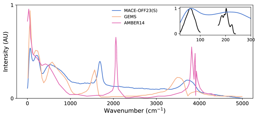
Figure 9: Protein in explicit solvent. Power spectrum of the high hydration state of crambin computed from 125 ps simulation. Inset shows correspondence of the MACE-OFF23(S) spectrum with the experimental spectrum for low wavenumber regions. GEMS and AMBER spectra are reproduced from Ref. [84].

III.7 Computational performance

To evaluate the computational performance of MACE-OFF23, we perform NVT molecular dynamics for water using the LAMMPS software, with simulation sizes ranging from $10^{2}$ to $10^{5}$ atoms. The results are summarized in Figure 10; all simulations were performed with the MACE-OFF23(S) model and utilized NVIDIA A100 GPUs. The LAMMPS evaluator relies on LibTorch (the C++ interface for PyTorch) and the Kokkos performance portability libraries.

The black curve in Figure 10 shows the computational performance as a function of system size for single-GPU evaluation, where performance is measured in units of millions of timesteps per day (equivalent to ns/day if the timestep is 1 fs). The model achieved 6.5 ns/day peak performance for roughly 200 atoms and 2.5 ns/day for roughly 1000 atoms, which is competitive with other machine learning force fields such as ANI [27] or AIMNet [8].

The three colored curves demonstrate the performance when multiple GPUs are employed to access larger systems with domain decomposition. Each has a dashed part which connects the single-GPU result (on the black curve) to the two-GPU result; the notable decrease in performance is explained by a different treatment of “ghost” atoms (those atoms which lie outside a given subdomain, but sufficiently near the boundary to influence “local” atoms). Without domain decomposition (assuming periodic boundary conditions), each ghost atom is a translation of a local atom—or, put differently, the full structure comprises a periodic graph—allowing for efficient reuse of intermediate calculations and better performance. Once the full domain is split across GPUs, it becomes more challenging to reuse intermediate results efficiently and, at present, some redundant calculations are performed. (The isolated colored dots show the single-GPU performance without efficient handling of ghost atoms). Finally, the solid colored lines demonstrate perfect weak scaling, where each subdomain belongs to one GPU, and the simulation speed is now independent of the system size.

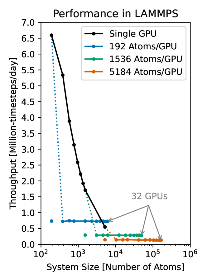
Figure 10: Computational performance. Performance of molecular dynamics with LAMMPS for liquid water in the NVT ensemble at 1 g/cm³ and 300 K with a 1 fs timestep. All simulations used the MACE-OFF23(S) model and one or more A100 GPUs. Single-GPU (the black line) refers to a “no domain decomposition” mode, where each configuration is provided to the MACE evaluator as a periodic graph (requiring custom processing of the LAMMPS neighbor list). Otherwise, domain decomposition is employed (colored lines), with one subdomain per GPU. The dashed parts of the colored lines reflect the transition between modes, and the isolated colored dots show the single-GPU performance without the more efficient “no domain decomposition” mode.

IV Outlook

In this paper, we presented the series of MACE-OFF23 models, demonstrating the broad applicability, transferability and capability of purely short-range machine learning potentials for organic (bio)molecular simulations. We have shown that models, based on the MACE higher order equivariant message passing architecture, can improve on the pioneering ANI models [27] that served as the only widely applicable machine learning force fields for molecules for a number of years. We have demonstrated significant improvements both in terms of accuracy and extrapolation combined with high computational speed.

The lack of explicit long-range interactions limits the domain of applicability of the present model to neutral, non-radical, and non-reactive systems. This is something that the recently published AIMNet-2 model aims to address by extending the ANI models to include charged species and long-range interactions [8]. We are currently working on a next-generation MACE-OFF model that will similarly include an explicit description of charges, enabling the description of amino acids with different protonation states, charged nucleic acids, and counter-ions. This will pave the way towards obtaining an accurate quantum mechanical transferable machine learning force field for simulating the full range of biologically relevant systems.

Contributions

DPK conceived the project, curated the training data, trained and evaluated the models, ran parts of the torsion drive tests, the molecular crystal tests, fitted the dipole and polarizability models, and wrote the initial draft. DPK and JHM implemented the OpenMM interface. JHM performed experiments on molecular liquids, peptides and proteins and wrote the initial draft. JTH implemented the MACE-torsion drive interfaces, and ran the DFT and force field torsion drives. VK ran the MD and PIMD simulations of water and molecular crystals and produced the IR and Raman spectra. IB and NJB implemented the accelerated custom kernels. WCW implemented the MACE-LAMMPS interface and benchmarked the model performance. IBM developed the intermolecular error analysis and evaluated the models. DJC and GC supervised the project. All authors discussed the results and edited the final manuscript.

V Supporting Information

V.1 Training details

Initially, the force weight in the loss was set to 1000 and the energy weight to 40. The learning rate was 0.01 and Adam optimizer with Amsgrad was used. The exponential moving average of the weights was taken in each training step. When the force error converged, the second phase of the training was started with force weight 10 and energy weight 1000 and the learning rate was reduced to 0.00025. Finally, the training was terminated when the energy error also stopped decreasing significantly. All models were trained on a single Nvidia A100 GPU. Training the small model took about 6 days, the medium about 10 days and the large model 14 days.

V.2 Test set errors

The numerical values of the test set errors are displayed in Table 3. Intermolecular force errors were obtained as RMSEs between DFT intermolecular forces and MACE predictions. The intermolecular forces were computed by summing over the translational and rotational components for each atom as shown in Ref. [63]. The algorithm can be summarized as follows:

Table 3: Summary of test set errors including inter-molecular force errors

			PubChem	DES370K Monomers	DES370K Dimers	Dipeptides	Solvated Amino Acids	Water	QMugs	Tripeptide
MAE	$\rm E$ $(\rm meV/at)$	Small	myblue!90 1.41	myblue!90 1.04	myblue!90 0.98	myblue!90 0.84	myblue!90 1.60	myblue!90 1.67	myblue!90 1.03	myblue!90 1.05
		Medium	mygreen!100 0.91	mygreen!100 0.63	mygreen!100 0.58	mygreen!100 0.52	mygreen!100 1.21	mygreen!100 0.76	mygreen!100 0.69	mygreen!100 0.57
		Large	myred!90 0.88	myred!90 0.59	myred!90 0.54	myred!90 0.42	myred!90 0.98	myred!90 0.83	myred!90 0.45	myred!90 0.38
	$\rm F_{total}$ $(\rm meV/\AA)$	Small	myblue!90 35.68	myblue!90 17.63	myblue!90 16.31	myblue!90 25.07	myblue!90 38.56	myblue!90 28.53	myblue!90 41.45	myblue!90 32.88
		Medium	mygreen!100 20.57	mygreen!100 9.36	mygreen!100 9.02	mygreen!100 14.27	mygreen!100 23.26	mygreen!100 15.27	mygreen!100 23.58	mygreen!100 18.74
		Large	myred!90 14.75	myred!90 6.58	myred!90 6.62	myred!90 10.19	myred!90 19.43	myred!90 13.57	myred!90 16.93	myred!90 13.20
	$\rm F_{inter}$ $(\rm meV/\AA)$	Small	myblue!90 0.13	myblue!90 0.18	myblue!90 3.01	myblue!90 0.07	myblue!90 16.98	myblue!90 19.03	myblue!90 0.09	myblue!90 0.07
		Medium	mygreen!100 0.13	mygreen!100 0.18	mygreen!100 1.79	mygreen!100 0.07	mygreen!100 10.30	mygreen!100 10.03	mygreen!100 0.09	mygreen!100 0.07
		Large	myred!90 0.13	myred!90 0.18	myred!90 1.44	myred!90 0.07	myred!90 8.85	myred!90 8.97	myred!90 0.09	myred!90 0.07
Relative MAE	$\rm E\leavevmode\nobreak\ (\%)$	Small	myblue!90 0.00	myblue!90 0.00	myblue!90 0.00	myblue!90 0.00	myblue!90 0.01	myblue!90 8.44	myblue!90 0.00	myblue!90 0.00
		Medium	mygreen!100 0.00	mygreen!100 0.00	mygreen!100 0.00	mygreen!100 0.00	mygreen!100 0.00	mygreen!100 3.84	mygreen!100 0.00	mygreen!100 0.00
		Large	myred!90 0.00	myred!90 0.00	myred!90 0.00	myred!90 0.00	myred!90 0.00	myred!90 4.18	myred!90 0.00	myred!90 0.00
	$\rm F_{total}\leavevmode\nobreak\ (\%)$	Small	myblue!90 4.65	myblue!90 2.72	myblue!90 3.46	myblue!90 3.55	myblue!90 3.16	myblue!90 4.50	myblue!90 4.12	myblue!90 3.66
		Medium	mygreen!100 2.68	mygreen!100 1.45	mygreen!100 1.91	mygreen!100 2.02	mygreen!100 1.90	mygreen!100 2.41	mygreen!100 2.35	mygreen!100 2.09
		Large	myred!90 1.92	myred!90 1.02	myred!90 1.40	myred!90 1.44	myred!90 1.59	myred!90 2.14	myred!90 1.68	myred!90 1.47
	$\rm F_{inter}\leavevmode\nobreak\ (\%)$	Small	myblue!90 nan	myblue!90 nan	myblue!90 15.52	myblue!90 nan	myblue!90 21.66	myblue!90 21.19	myblue!90 nan	myblue!90 nan
		Medium	mygreen!100 nan	mygreen!100 nan	mygreen!100 9.25	mygreen!100 nan	mygreen!100 13.14	mygreen!100 11.17	mygreen!100 nan	mygreen!100 nan
		Large	myred!90 nan	myred!90 nan	myred!90 7.44	myred!90 nan	myred!90 11.29	myred!90 9.99	myred!90 nan	myred!90 nan
RMSE	$\rm E$ $(\rm meV/at)$	Small	myblue!90 2.74	myblue!90 1.47	myblue!90 1.51	myblue!90 1.26	myblue!90 1.98	myblue!90 2.07	myblue!90 1.28	myblue!90 1.40
		Medium	mygreen!100 2.02	mygreen!100 0.90	mygreen!100 0.91	mygreen!100 0.85	mygreen!100 1.55	mygreen!100 0.99	mygreen!100 0.89	mygreen!100 0.75
		Large	myred!90 2.48	myred!90 0.84	myred!90 0.87	myred!90 0.70	myred!90 1.32	myred!90 0.99	myred!90 0.58	myred!90 0.49
	$\rm F_{total}$ $(\rm meV/\AA)$	Small	myblue!90 61.83	myblue!90 26.15	myblue!90 28.48	myblue!90 36.97	myblue!90 53.55	myblue!90 39.33	myblue!90 62.46	myblue!90 71.41
		Medium	mygreen!100 40.51	mygreen!100 14.31	mygreen!100 16.81	mygreen!100 22.25	mygreen!100 32.19	mygreen!100 21.40	mygreen!100 36.73	mygreen!100 33.94
		Large	myred!90 33.34	myred!90 10.27	myred!90 12.81	myred!90 16.19	myred!90 26.91	myred!90 18.78	myred!90 27.17	myred!90 22.46
	$\rm F_{inter}$ $(\rm meV/\AA)$	Small	myblue!90 0.78	myblue!90 0.44	myblue!90 8.70	myblue!90 0.13	myblue!90 27.11	myblue!90 27.59	myblue!90 0.17	myblue!90 0.12
		Medium	mygreen!100 0.79	mygreen!100 0.44	mygreen!100 5.54	mygreen!100 0.13	mygreen!100 16.46	mygreen!100 15.05	mygreen!100 0.17	mygreen!100 0.12
		Large	myred!90 0.76	myred!90 0.44	myred!90 4.34	myred!90 0.13	myred!90 14.24	myred!90 13.39	myred!90 0.17	myred!90 0.12
Relative RMSE	$\rm E\leavevmode\nobreak\ (\%)$	Small	myblue!90 0.00	myblue!90 0.00	myblue!90 0.00	myblue!90 0.00	myblue!90 0.01	myblue!90 8.30	myblue!90 0.00	myblue!90 0.00
		Medium	mygreen!100 0.00	mygreen!100 0.00	mygreen!100 0.00	mygreen!100 0.00	mygreen!100 0.00	mygreen!100 3.96	mygreen!100 0.00	mygreen!100 0.00
		Large	myred!90 0.00	myred!90 0.00	myred!90 0.00	myred!90 0.00	myred!90 0.00	myred!90 3.98	myred!90 0.00	myred!90 0.00
	$\rm F_{total}\leavevmode\nobreak\ (\%)$	Small	myblue!90 5.56	myblue!90 2.79	myblue!90 4.13	myblue!90 3.63	myblue!90 3.47	myblue!90 4.58	myblue!90 4.66	myblue!90 5.45
		Medium	mygreen!100 3.64	mygreen!100 1.52	mygreen!100 2.44	mygreen!100 2.19	mygreen!100 2.09	mygreen!100 2.49	mygreen!100 2.74	mygreen!100 2.59
		Large	myred!90 3.00	myred!90 1.09	myred!90 1.86	myred!90 1.59	myred!90 1.74	myred!90 2.19	myred!90 2.03	myred!90 1.71
	$\rm F_{inter}\leavevmode\nobreak\ (\%)$	Small	myblue!90 nan	myblue!90 nan	myblue!90 8.95	myblue!90 nan	myblue!90 20.17	myblue!90 20.18	myblue!90 nan	myblue!90 nan
		Medium	mygreen!100 nan	mygreen!100 nan	mygreen!100 5.70	mygreen!100 nan	mygreen!100 12.25	mygreen!100 11.00	mygreen!100 nan	mygreen!100 nan
		Large	myred!90 nan	myred!90 nan	myred!90 4.46	myred!90 nan	myred!90 10.60	myred!90 9.79	myred!90 nan	myred!90 nan

1. identify molecules (labeled $j$)

2. within each molecule $j$ sum over all atomic forces (labeled $k$) to obtain the translational component:

   $$F^{\rm trans}_{j}=\sum_{k\in j}f_{k}$$ (9)

3. redistribute the molecular translational force onto individual atoms (labeled $i$) to obtain the atomic translational contributions:

   $$f^{\rm trans}_{i}=\frac{m_{i}}{M_{j}}F^{\rm trans}_{j}$$ (10)

   where $m_{i}$ are atomic masses and $M_{j}$ are molecular masses

4. similarly, compute the torque on the entire molecule:

   $$T_{j}=\sum_{k\in j}f_{k}\times\left(r_{k}-R^{\rm com}_{j}\right)$$ (11)

5. compute the rotational atomic force contributions that give rise to the given molecular torque:

   $$f^{\rm rot}_{i}=m_{i}\left(r_{i}-R^{\rm com}_{j}\right)\times(I_{j}^{\alpha\beta})^{-1}T_{j}$$ (12)

   where $I_{j}^{\alpha\beta}$ are the molecular moments of inertia

6. compute the vibrational contribution as the difference:

   $$f^{\rm vib}_{i}=f_{i}-f^{\rm trans}_{i}-f^{\rm rot}_{i}$$ (13)

7. the intermolecular force is calculated as the sum of the translational and rotational contributions.

Relative errors were obtained by dividing the absolute errors by the typical DFT force magnitudes:

$$\mathrm{Rel\leavevmode\nobreak\ MAE}=\frac{\sum_{i}|f^{DFT}_{i}-f^{MACE}_{i}|}{\sum_{i}|f^{DFT}_{i}-{\bar{f}^{DFT}}|}$$ (14)

$$\mathrm{Rel\leavevmode\nobreak\ RMSE}=\sqrt{\frac{\sum_{i}(f^{DFT}_{i}-f^{MACE}_{i})^{2}}{\sum_{i}(f^{DFT}_{i}-{\bar{f}^{DFT}})^{2}}}$$ (15)

where $\bar{f}^{DFT}=\sum_{i}f_{i}^{DFT}$/N is the average DFT force (often zero).

Table 3 shows these errors computed for all three MACE models on each category of atomic configurations found in the test set. Interestingly, even though PubChem, DES370K Monomers, Dipeptides, QMugs and Tripeptides comprise only isolated molecule configurations, we find a small error that is incorrectly attributed to intermolecular interactions. This issue arises because DFT forces in these test data to not obey translational and rotational symmetry, i.e. total molecular force and torque do not sum to zero, even though a single molecule is present in each simulation box. Meanwhile, MACE forces do obey these symmetries, and therefore the difference shows up as an intermolecular error which is identical for all three MACE models.

The code used for this analysis is made available on https://github.com/imagdau/aseMolec.git.

V.3 Computational experiment details

V.3.1 Torsion angle scanning calculations

The TorsionNet-500 [67] and biaryl torsion [66] benchmark datasets were recomputed at the SPICE [50] level of QM theory (B97M-D3(BJ)/def2-TZVPPD [51, 52, 53, 54, 55]) to assess the accuracy of the MACE models in predicting the potential energy surfaces of rotatable bonds commonly found in drug-like molecules. Starting from the published optimized geometries, a torsion scan was performed using TorsionDrive [85] via its interface with QCEngine [86]. The dihedral angles were scanned in 15^∘ increments and each constrained geometry optimization was carried out with geomeTRIC [87], using PSI4 [56] to calculate the DFT energies and forces. For each of the assessed force field models, a separate constrained geometry optimization was performed starting from the DFT reference geometries and holding the target torsion fixed at each grid point value. The final RMSD between the optimized and reference geometry was recorded, along with the energy to calculate the potential energy surfaces.

V.3.2 Paracetamol spectra

To compute the vibrational spectrum for the paracetamol form II polymorph, we first performed a 20 ps path-integral MD simulation using the MACE-OFF23(S) model at 500 K, following the prescriptions of the Path Integral coarse-Grained Simulations (PIGS) approach [68, 69]. The path-integral MD simulations are performed with a 0.50 fs timestep using the BAOAB integration scheme extended to path-integral MD [88] using the path-integral Langevin equation thermostats [89] with a time constant of 100 fs.

To generate a potential energy surface that effectively encodes quantum nuclear effects, we followed the PIGS technique. We used the positions and forces on the centroid of the path-integral to fit a MACE model that represents the difference between the potential energy surface and the potential of mean force on the centroid at an elevated temperature of 500 K. The sum of MACE-OFF23(S) and the PIGS model gives a transferable effective potential energy surface that encodes quantum nuclear effects.

To generate a trajectory with quantum nuclear motion, we run MD with the sum of MACE-OFF23(S) and the PIGS model using the i-PI [90] software to propagate the equations of motion and the ASE calculator as the force-provider. The MD simulations were performed with a 0.50 fs timestep using a weak global stochastic velocity rescaling thermostat. To generate classical trajectories we perform MD with the same setup but without the PIGS potential.

We predicted the $L=0$ and $L=2$ spherical harmonic components of polarizability tensors on the trajectories and computed their time correlation functions to obtain the isotropic and anisotropic Raman spectra [68]. We estimate the powder Raman spectrum as a linear combination of the isotropic and the anisotropic Raman spectra [91].

V.3.3 Condensed phase simulations

Initial PDB files were taken from Ref. [79] and periodic boxes were generated using packmol [92]. Boxes were prepared containing 64 molecules, with box vectors determined such that the initial density was 80% of the experimental density. Structures were minimized with the L-BFGS algorithm prior to MD. Molecular dynamics were performed with OpenMM, using a custom fork of the openmm-ml package to interface MACE models to the MD code. Simulations were performed in the NPT ensemble. The Langevin equations of motion were integrated with a timestep of 1 fs and a Monte Carlo barostat was used to maintain pressure at 1 atm. Temperatures were maintained at 298 K except for those compounds whose boiling point was below this value, for which a value of 10 K below the experimental boiling point was used. Dynamics were propagated for 300 ps, and the final density was calculated by averaging over the final 500 frames of the simulation.

Heat of vaporization calculations additionally required simulation of the isolated molecule in the vacuum phase, which was carried out on a nonperiodic molecule. Final energies for both condensed and vacuum phases were calculated by averaging over the final 500 frames of each trajectory.

The computational details for simulating the classical and quantum dynamical properties of water are the same as the setup for paracetamol (see the previous section).

	MAE	RMSE	$r^{2}$
MACE-OFF23(S)	0.23	0.38	-0.86
MACE-OFF23(M)	0.09	0.15	0.73
ANI-2x	0.21	0.36	-2.13

Table 4: Summary of density errors

	MAE	RMSE	$r^{2}$
MACE-OFF23(S)	1.48	2.19	0.86
MACE-OFF23(M)	2.18	2.53	0.87
ANI-2x	2.75	3.45	0.66

Table 5: Summary of $\Delta H_{vap}$ errors

Figure 11 shows the variation of the density of water as a function of temperature.

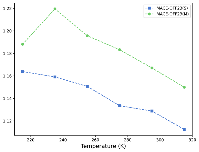
Figure 11: Water density / temperature curves for MACE-OFF23(S) and MACE-OFF23(M).

V.3.4 Ala₃ Free Energy Surface

Molecular dynamics simulations were performed with OpenMM, as in the previous section. Enhanced sampling simulations were performed with metadynamics. Two collective variables were defined by the two torsion angles on the backbone of the central alanine residue. A 1 ns simulation was performed with a temperature bias factor of 10, a barrier height of 1 kJ/mol and a frequency of 100 steps.

V.3.5 Crambin in explicit solvent

Crambin was prepared from the PDB structure 1EJG. The initial structure was prepared using pdbfixer [93] and solvated in an orthorombic box with padding between solute and the box edge set to 1.2 nm. Dynamics were performed in the NPT emsemble, with pressure maintained at 1 atm with a Monte Carlo barostat, as implemented in OpenMM. A 1 fs timestep was used both for integrating the Langevin equations of motion and for writing the trajectory to disk for post processing. The power spectrum was calculated as the fourier transform of the velocity autocorrelation function using the Travis program with default settings [94, 95, 96, 97].

V.4 Equivariant dielectric fitting

To produce the paracetamol and water spectra we used a MACE model to predict the dipoles and polarizabilities along the MACE-OFF23 generated MD trajectories. The model architecture was identical to the MACE architecture described above, with the only difference being the readout function producing a vector and a tensor (dipole and polarisability) for each atom, instead of the atomic site energies. A relatively small MACE model is already capable of achieving high accuracy predictions, and the selected models used the hyperparameters displayed in Table 6.

Table 6: Hyperparameters of the MACE models for dipoles and polarizabilities

	Paracetamol	Water
Cutoff radius (Å)	5.0	6.0
Chemical channels	16	32
$k$ (Eq. (1))
max L (Eq. (5))	2	2

V.5 Lattice enthalpies

First, the internal energy of the crystalline form was computed under the harmonic approximation:

$$U(T) =\left(\frac{\partial\ln{Z}}{\partial\frac{1}{k_{B}T}}\right)$$ (16)

$$=E_{\text{MACE}}+\int_{0}^{\infty}\left[\frac{\epsilon}{e^{\frac{\epsilon}{k_{B}T}}-1}+\frac{\epsilon}{2}\right]\sigma(\epsilon)\text{d}\epsilon$$

where $Z$ denotes the partition function of the system, and $\sigma(\epsilon)$ represents the degeneracy or phonon density of states as a function of vibrational energy. The above expression contains an electronic contribution, computed using MACE, a zero point energy contribution, and a contribution from finite-temperature vibrational energy. To compute the vibrational contribution, we used a $3\times 3\times 3$ supercell for all the molecules considered. For the gaseous form of the molecules, we employed the ideal gas approximation to compute the enthalpies of the gas as:

$$U(T)=e_{\text{MACE}}+E_{\text{ZPE}}+\int_{0}^{T}C_{p}\text{d}T$$ (17)

where we used the ideal gas value to evaluate the last term, giving $4RT$ for all system except for the linear carbon-dioxide, where the value is $3.5RT$.

Combining the above two expressions, we can compute the sublimation enthalpies as:

$$\Delta H_{\text{subm}} =U_{\text{gas}}(T)-U_{\text{cryst}}(T)$$ (18)

$$=E_{\text{latt}}+\Delta E_{\text{vib}}+4RT$$

To assess the accuracy of the MACE model we used the X23 set of molecular crystals [74]. We first relaxed the cells, followed by phonon and normal mode calculations to obtain the finite temperature vibrational as well as zero point contributions to the enthalpies, following the protocol above. It is important to note that for the ANI-2x force field it was not possible to fully relax the crystal geometries, because the model cannot predict stresses. Hence, we kept the cell fixed at the DFT equilibrium values from Ref. [74]. The results are summarized in Table 7.

Table 7: Sublimation enthalphy in kJ/mol

System	$\Delta H_{\text{sub}}^{0}$ exp.	$\Delta H_{\text{sub}}^{0}$ MACE-OFF23(L)	$\Delta H_{\text{sub}}^{0}$ ANI-2x
1,4-Cyclohexanedione	81.1	85.1	59.7
Acetic acid	67.7	70.3	90.7
Adamantane	61.6	69.2	67.1
Ammonia	31.2	26.8	23.0
Anthracene	101.9	106.3	98.9
Benzene	44.9	58.4	48.3
Carbon dioxide	26.1	4.1	-117.9
Cyanamide	75.5	87.3	36.9
Cytosine	156.4	143.2	118.6
Ethyl carbamate	78.8	91.4	77.0
Formamide	71.7	80.1	67.3
Hexamine	75.8	62.3	83.5
Imidazole	81.4	86.3	86.6
Naphthalene	72.6	83.6	72.4
Oxalic acid	93.7	89.7	44.1
Oxalic acid	93.6	93.5	45.4
Pyrazine	56.3	69.7	53.7
Pyrazole	72.4	73.0	75.4
s-Triazine	55.7	75.6	112.1
s-Trioxane	56.3	53.9	51.7
Succinic acid	123.1	123.5	141.7
Uracil	129.2	131.8	98.9
Urea	93.8	112.5	78.2

V.6 Crystal structure geometries

In Table 8 we compare the MACE-OFF23(L) relaxed crystal structure lattice parameters with the experimental ones reported in Ref. [75]. We confirm that MACE is able to accurately reproduce the lattice constant of molecular crystals purely trained on molecular dimers. Additional trimer training data, or a higher level of reference theory, such as coupled cluster, could probably further improve the agreement with experiments.

Table 8: Crystal structure geometries

Molecule	$T_{\text{exp}}$		Experiment	MACE-OFF23(L)
Acetic acid	40	$a$	13.151	13.359
		$b$	3.923	3.809
		$c$	5.762	5.542
		$V$	297.27	282.01
Ammonia	2	$a$	5.048	4.946
		$V$	128.63	120.98
Benzene	4	$a$	7.351	6.59
		$b$	9.364	9.303
		$c$	6.695	6.851
		$V$	460.84	420.51
Naphthalene	10	$a$	8.0846	7.821
		$b$	5.9375	5.836
		$c$	8.6335	8.430
		$\beta$	124.67	125.26
		$V$	340.83	314.23
Pyrazine	184	$a$	9.325	9.351
		$b$	5.850	5.508
		$c$	3.733	3.545
		$V$	203.64	182.57
Urea	40	$a$	5.565	5.330
		$c$	4.684	4.670
		$V$	145.06	123.68

References

- Lysogorskiy et al. [2021] Y. Lysogorskiy, C. v. d. Oord, A. Bochkarev, S. Menon, M. Rinaldi, T. Hammerschmidt, M. Mrovec, A. Thompson, G. Csányi, C. Ortner, et al., Performant implementation of the atomic cluster expansion (pace) and application to copper and silicon, npj computational materials 7, 97 (2021).
- Batatia et al. [2022a] I. Batatia, D. P. Kovacs, G. Simm, C. Ortner, and G. Csányi, Mace: Higher order equivariant message passing neural networks for fast and accurate force fields, Advances in Neural Information Processing Systems 35, 11423 (2022a).
- Kovács et al. [2023] D. P. Kovács, I. Batatia, E. S. Arany, and G. Csányi, Evaluation of the MACE force field architecture: From medicinal chemistry to materials science, The Journal of Chemical Physics 159, 044118 (2023).
- Batzner et al. [2022] S. Batzner, A. Musaelian, L. Sun, M. Geiger, J. P. Mailoa, M. Kornbluth, N. Molinari, T. E. Smidt, and B. Kozinsky, E (3)-equivariant graph neural networks for data-efficient and accurate interatomic potentials, Nature communications 13, 2453 (2022).
- Zaverkin et al. [2023] V. Zaverkin, D. Holzmüller, L. Bonfirraro, and J. Kästner, Transfer learning for chemically accurate interatomic neural network potentials, Physical Chemistry Chemical Physics 25, 5383 (2023).
- Haghighatlari et al. [2022] M. Haghighatlari, J. Li, X. Guan, O. Zhang, A. Das, C. J. Stein, F. Heidar-Zadeh, M. Liu, M. Head-Gordon, L. Bertels, et al., Newtonnet: A newtonian message passing network for deep learning of interatomic potentials and forces, Digital Discovery 1, 333 (2022).
- Shapeev [2016] A. V. Shapeev, Moment tensor potentials: A class of systematically improvable interatomic potentials, Multiscale Modeling & Simulation 14, 1153 (2016).
- Anstine et al. [2023] D. Anstine, R. Zubatyuk, and O. Isayev, Aimnet2: A neural network potential to meet your neutral, charged, organic, and elemental-organic needs, ChemRxiv 10.26434/chemrxiv-2023-296ch (2023).
- Kabylda et al. [2023] A. Kabylda, V. Vassilev-Galindo, S. Chmiela, I. Poltavsky, and A. Tkatchenko, Efficient interatomic descriptors for accurate machine learning force fields of extended molecules, Nature Communications 14, 3562 (2023).
- Behler [2021] J. Behler, Four generations of high-dimensional neural network potentials, Chemical Reviews 121, 10037 (2021).
- Musil et al. [2021] F. Musil, A. Grisafi, A. P. Bartók, C. Ortner, G. Csányi, and M. Ceriotti, Physics-inspired structural representations for molecules and materials, Chemical Reviews 121, 9759 (2021).
- Deringer et al. [2021a] V. L. Deringer, A. P. Bartók, N. Bernstein, D. M. Wilkins, M. Ceriotti, and G. Csányi, Gaussian process regression for materials and molecules, Chemical Reviews 121, 10073 (2021a).
- Huang and Von Lilienfeld [2021] B. Huang and O. A. Von Lilienfeld, Ab initio machine learning in chemical compound space, Chemical reviews 121, 10001 (2021).
- Daw and Baskes [1984] M. S. Daw and M. I. Baskes, Embedded-atom method: Derivation and application to impurities, surfaces, and other defects in metals, Physical Review B 29, 6443 (1984).
- Deringer et al. [2021b] V. L. Deringer, N. Bernstein, G. Csányi, C. Ben Mahmoud, M. Ceriotti, M. Wilson, D. A. Drabold, and S. R. Elliott, Origins of structural and electronic transitions in disordered silicon, Nature 589, 59 (2021b).
- Baldwin et al. [2023] W. J. Baldwin, X. Liang, J. Klarbring, M. Dubajic, D. Dell’Angelo, C. Sutton, C. Caddeo, S. D. Stranks, A. Mattoni, A. Walsh, et al., Dynamic local structure in caesium lead iodide: Spatial correlation and transient domains, Small , 2303565 (2023).
- Rosenbrock et al. [2021] C. W. Rosenbrock, K. Gubaev, A. V. Shapeev, L. B. Pártay, N. Bernstein, G. Csányi, and G. L. Hart, Machine-learned interatomic potentials for alloys and alloy phase diagrams, npj Computational Materials 7, 24 (2021).
- Zhou et al. [2023] Y. Zhou, W. Zhang, E. Ma, and V. L. Deringer, Device-scale atomistic modelling of phase-change memory materials, Nature Electronics , 1 (2023).
- Dauber-Osguthorpe and Hagler [2019] P. Dauber-Osguthorpe and A. T. Hagler, Biomolecular force fields: where have we been, where are we now, where do we need to go and how do we get there?, J Comput Aided Mol Des 33, 133–203 (2019).
- Hagler [2019] A. T. Hagler, Force field development phase ii: Relaxation of physics-based criteria… or inclusion of more rigorous physics into the representation of molecular energetics, J Comput Aided Mol Des 33, 205–264 (2019).
- Boothroyd et al. [2023] S. Boothroyd, P. K. Behara, O. C. Madin, D. F. Hahn, H. Jang, V. Gapsys, J. R. Wagner, J. T. Horton, D. L. Dotson, M. W. Thompson, J. Maat, T. Gokey, L.-P. Wang, D. J. Cole, M. K. Gilson, J. D. Chodera, C. I. Bayly, M. R. Shirts, and D. L. Mobley, Development and benchmarking of open force field 2.0.0: The sage small molecule force field, J. Chem. Theory Comput. 0, null (2023), pMID: 37167319.
- Gapsys et al. [2020] V. Gapsys, L. Pérez-Benito, M. Aldeghi, D. Seeliger, H. Van Vlijmen, G. Tresadern, and B. L. De Groot, Large scale relative protein ligand binding affinities using non-equilibrium alchemy, Chem. Sci. 11, 1140 (2020).
- Bannwarth et al. [2019] C. Bannwarth, S. Ehlert, and S. Grimme, Gfn2-xtb—an accurate and broadly parametrized self-consistent tight-binding quantum chemical method with multipole electrostatics and density-dependent dispersion contributions, Journal of chemical theory and computation 15, 1652 (2019).
- Smith et al. [2017a] J. S. Smith, O. Isayev, and A. E. Roitberg, Ani-1: an extensible neural network potential with dft accuracy at force field computational cost, Chemical science 8, 3192 (2017a).
- Smith et al. [2018] J. S. Smith, B. Nebgen, N. Lubbers, O. Isayev, and A. E. Roitberg, Less is more: Sampling chemical space with active learning, The Journal of chemical physics 148, 241733 (2018).
- Smith et al. [2019] J. S. Smith, B. T. Nebgen, R. Zubatyuk, N. Lubbers, C. Devereux, K. Barros, S. Tretiak, O. Isayev, and A. E. Roitberg, Approaching coupled cluster accuracy with a general-purpose neural network potential through transfer learning, Nature communications 10, 1 (2019).
- Devereux et al. [2020] C. Devereux, J. S. Smith, K. K. Huddleston, K. Barros, R. Zubatyuk, O. Isayev, and A. E. Roitberg, Extending the applicability of the ani deep learning molecular potential to sulfur and halogens, Journal of Chemical Theory and Computation 16, 4192 (2020).
- Zubatyuk et al. [2019] R. Zubatyuk, J. S. Smith, J. Leszczynski, and O. Isayev, Accurate and transferable multitask prediction of chemical properties with an atoms-in-molecules neural network, Science advances 5, eaav6490 (2019).
- Zubatyuk et al. [2021] R. Zubatyuk, J. S. Smith, B. T. Nebgen, S. Tretiak, and O. Isayev, Teaching a neural network to attach and detach electrons from molecules, Nature Communications 12, 4870 (2021).
- Behler and Parrinello [2007] J. Behler and M. Parrinello, Generalized neural-network representation of high-dimensional potential-energy surfaces, Physical review letters 98, 146401 (2007).
- Smith et al. [2017b] J. S. Smith, O. Isayev, and A. E. Roitberg, Ani-1, a data set of 20 million calculated off-equilibrium conformations for organic molecules, Scientific data 4, 1 (2017b).
- Smith et al. [2020a] J. S. Smith, R. Zubatyuk, B. Nebgen, N. Lubbers, K. Barros, A. E. Roitberg, O. Isayev, and S. Tretiak, The ani-1ccx and ani-1x data sets, coupled-cluster and density functional theory properties for molecules, Scientific data 7, 134 (2020a).
- Inizan et al. [2023] T. J. Inizan, T. Plé, O. Adjoua, P. Ren, H. Gökcan, O. Isayev, L. Lagardère, and J.-P. Piquemal, Scalable hybrid deep neural networks/polarizable potentials biomolecular simulations including long-range effects, Chemical Science 14, 5438 (2023).
- Tu et al. [2023] N. T. P. Tu, N. Rezajooei, E. R. Johnson, and C. Rowley, A neural network potential with rigorous treatment of long-range dispersion, Digital Discovery (2023).
- Gilmer et al. [2017] J. Gilmer, S. S. Schoenholz, P. F. Riley, O. Vinyals, and G. E. Dahl, Neural message passing for quantum chemistry, in International conference on machine learning (PMLR, 2017) pp. 1263–1272.
- Unke and Meuwly [2019] O. T. Unke and M. Meuwly, Physnet: A neural network for predicting energies, forces, dipole moments, and partial charges, Journal of chemical theory and computation 15, 3678 (2019).
- Plé et al. [2023] T. Plé , L. Lagardère, and J.-P. Piquemal, Force-field-enhanced neural network interactions: from local equivariant embedding to atom-in-molecule properties and long-range effects, Chemical Science 10.1039/d3sc02581k (2023).
- Thürlemann and Riniker [2023] M. Thürlemann and S. Riniker, Hybrid classical/machine-learning force fields for the accurate description of molecular condensed-phase systems, Chemical Science 14, 12661 (2023).
- Unke et al. [2022a] O. T. Unke, M. Stöhr, S. Ganscha, T. Unterthiner, H. Maennel, S. Kashubin, D. Ahlin, M. Gastegger, L. M. Sandonas, A. Tkatchenko, and K.-R. Müller, Accurate machine learned quantum-mechanical force fields for biomolecular simulations (2022a), arXiv:2205.08306 .
- Unke et al. [2021] O. T. Unke, S. Chmiela, M. Gastegger, K. T. Schütt, H. E. Sauceda, and K.-R. Müller, Spookynet: Learning force fields with electronic degrees of freedom and nonlocal effects, Nature communications 12, 7273 (2021).
- Schütt et al. [2017] K. Schütt, P.-J. Kindermans, H. E. Sauceda Felix, S. Chmiela, A. Tkatchenko, and K.-R. Müller, Schnet: A continuous-filter convolutional neural network for modeling quantum interactions, Advances in neural information processing systems 30 (2017).
- Schütt et al. [2021] K. Schütt, O. Unke, and M. Gastegger, Equivariant message passing for the prediction of tensorial properties and molecular spectra, in International Conference on Machine Learning (PMLR, 2021) pp. 9377–9388.
- Gasteiger et al. [2021] J. Gasteiger, F. Becker, and S. Günnemann, Gemnet: Universal directional graph neural networks for molecules, Advances in Neural Information Processing Systems 34, 6790 (2021).
- Willatt et al. [2018] M. J. Willatt, F. Musil, and M. Ceriotti, Feature optimization for atomistic machine learning yields a data-driven construction of the periodic table of the elements, Physical Chemistry Chemical Physics 20, 29661 (2018).
- Darby et al. [2023a] J. P. Darby, D. P. Kovács, I. Batatia, M. A. Caro, G. L. Hart, C. Ortner, and G. Csányi, Tensor-reduced atomic density representations, Physical Review Letters 131, 028001 (2023a).
- Wigner [2012] E. Wigner, Group theory: and its application to the quantum mechanics of atomic spectra, Vol. 5 (Elsevier, 2012).
- Dusson et al. [2022] G. Dusson, M. Bachmayr, G. Csányi, R. Drautz, S. Etter, C. van der Oord, and C. Ortner, Atomic cluster expansion: Completeness, efficiency and stability, Journal of Computational Physics 454, 110946 (2022).
- Batatia et al. [2022b] I. Batatia, S. Batzner, D. P. Kovács, A. Musaelian, G. N. Simm, R. Drautz, C. Ortner, B. Kozinsky, and G. Csányi, The design space of e (3)-equivariant atom-centered interatomic potentials, arXiv preprint arXiv:2205.06643 (2022b).
- Kovács et al. [2021] D. P. Kovács, C. v. d. Oord, J. Kucera, A. E. Allen, D. J. Cole, C. Ortner, and G. Csányi, Linear atomic cluster expansion force fields for organic molecules: beyond rmse, Journal of chemical theory and computation 17, 7696 (2021).
- Eastman et al. [2023] P. Eastman, P. K. Behara, D. L. Dotson, R. Galvelis, J. E. Herr, J. T. Horton, Y. Mao, J. D. Chodera, B. P. Pritchard, Y. Wang, et al., Spice, a dataset of drug-like molecules and peptides for training machine learning potentials, Scientific Data 10, 11 (2023).
- Najibi and Goerigk [2018] A. Najibi and L. Goerigk, The nonlocal kernel in van der waals density functionals as an additive correction: An extensive analysis with special emphasis on the b97m-v and b97m-v approaches, Journal of Chemical Theory and Computation 14, 5725 (2018).
- Weigend and Ahlrichs [2005] F. Weigend and R. Ahlrichs, Balanced basis sets of split valence, triple zeta valence and quadruple zeta valence quality for h to rn: Design and assessment of accuracy, Physical Chemistry Chemical Physics 7, 3297 (2005).
- Rappoport and Furche [2010] D. Rappoport and F. Furche, Property-optimized gaussian basis sets for molecular response calculations, The Journal of chemical physics 133 (2010).
- Grimme et al. [2011] S. Grimme, S. Ehrlich, and L. Goerigk, Effect of the damping function in dispersion corrected density functional theory, Journal of computational chemistry 32, 1456 (2011).
- Grimme et al. [2010] S. Grimme, J. Antony, S. Ehrlich, and H. Krieg, A consistent and accurate ab initio parametrization of density functional dispersion correction (dft-d) for the 94 elements h-pu, The Journal of chemical physics 132 (2010).
- Smith et al. [2020b] D. G. Smith, L. A. Burns, A. C. Simmonett, R. M. Parrish, M. C. Schieber, R. Galvelis, P. Kraus, H. Kruse, R. Di Remigio, A. Alenaizan, et al., Psi4 1.4: Open-source software for high-throughput quantum chemistry, The Journal of chemical physics 152 (2020b).
- Maier et al. [2015] J. A. Maier, C. Martinez, K. Kasavajhala, L. Wickstrom, K. E. Hauser, and C. Simmerling, ff14sb: improving the accuracy of protein side chain and backbone parameters from ff99sb, Journal of chemical theory and computation 11, 3696 (2015).
- Donchev et al. [2021] A. G. Donchev, A. G. Taube, E. Decolvenaere, C. Hargus, R. T. McGibbon, K.-H. Law, B. A. Gregersen, J.-L. Li, K. Palmo, K. Siva, et al., Quantum chemical benchmark databases of gold-standard dimer interaction energies, Scientific data 8, 55 (2021).
- Isert et al. [2022] C. Isert, K. Atz, J. Jiménez-Luna, and G. Schneider, Qmugs, quantum mechanical properties of drug-like molecules, Scientific Data 9, 273 (2022).
- Darby et al. [2023b] J. P. Darby, D. P. Kovács, I. Batatia, M. A. Caro, G. L. Hart, C. Ortner, and G. Csányi, Tensor-reduced atomic density representations, Physical Review Letters 131, 028001 (2023b).
- Schran et al. [2021] C. Schran, F. L. Thiemann, P. Rowe, E. A. Müller, O. Marsalek, and A. Michaelides, Machine learning potentials for complex aqueous systems made simple, Proceedings of the National Academy of Sciences 118, e2110077118 (2021).
- Paszke et al. [2019] A. Paszke, S. Gross, F. Massa, A. Lerer, J. Bradbury, G. Chanan, T. Killeen, Z. Lin, N. Gimelshein, L. Antiga, A. Desmaison, A. Köpf, E. Yang, Z. DeVito, M. Raison, A. Tejani, S. Chilamkurthy, B. Steiner, L. Fang, J. Bai, and S. Chintala, Pytorch: An imperative style, high-performance deep learning library, in Neural Information Processing Systems (2019).
- Magdău et al. [2023] I.-B. Magdău, D. J. Arismendi-Arrieta, H. E. Smith, C. P. Grey, K. Hermansson, and G. Csányi, Machine learning force fields for molecular liquids: Ethylene carbonate/ethyl methyl carbonate binary solvent, npj Computational Materials 9, 146 (2023).
- Horton et al. [2022] J. T. Horton, S. Boothroyd, J. Wagner, J. A. Mitchell, T. Gokey, D. L. Dotson, P. K. Behara, V. K. Ramaswamy, M. Mackey, J. D. Chodera, et al., Open force field bespokefit: Automating bespoke torsion parametrization at scale, Journal of Chemical Information and Modeling 62, 5622 (2022).
- Hao et al. [2022] D. Hao, X. He, A. E. Roitberg, S. Zhang, and J. Wang, Development and evaluation of geometry optimization algorithms in conjunction with ani potentials, Journal of Chemical Theory and Computation 18, 978 (2022).
- Lahey et al. [2020] S.-L. J. Lahey, T. N. Thien Phuc, and C. N. Rowley, Benchmarking force field and the ani neural network potentials for the torsional potential energy surface of biaryl drug fragments, Journal of Chemical Information and Modeling 60, 6258 (2020).
- Rai et al. [2022] B. K. Rai, V. Sresht, Q. Yang, R. Unwalla, M. Tu, A. M. Mathiowetz, and G. A. Bakken, Torsionnet: A deep neural network to rapidly predict small-molecule torsional energy profiles with the accuracy of quantum mechanics, Journal of Chemical Information and Modeling 62, 785 (2022).
- Kapil et al. [2023] V. Kapil, D. P. Kovács, G. Csányi, and A. Michaelides, First-principles spectroscopy of aqueous interfaces using machine-learned electronic and quantum nuclear effects, Faraday Discussions 10.1039/d3fd00113j (2023).
- Musil et al. [2022] F. Musil, I. Zaporozhets, F. Noé, C. Clementi, and V. Kapil, Quantum dynamics using path integral coarse-graining, The Journal of Chemical Physics 157, 10.1063/5.0120386 (2022).
- Raimbault et al. [2019a] N. Raimbault, A. Grisafi, M. Ceriotti, and M. Rossi, Using gaussian process regression to simulate the vibrational raman spectra of molecular crystals, New Journal of Physics 21, 105001 (2019a).
- Raimbault et al. [2019b] N. Raimbault, A. Grisafi, M. Ceriotti, and M. Rossi, Using gaussian process regression to simulate the vibrational raman spectra of molecular crystals, New Journal of Physics 21, 105001 (2019b).
- Kolesov et al. [2011] B. A. Kolesov, M. A. Mikhailenko, and E. V. Boldyreva, Dynamics of the intermolecular hydrogen bonds in the polymorphs of paracetamol in relation to crystal packing and conformational transitions: a variable-temperature polarized raman spectroscopy study, Physical Chemistry Chemical Physics 13, 14243 (2011).
- Raimbault et al. [2019c] N. Raimbault, V. Athavale, and M. Rossi, Anharmonic effects in the low-frequency vibrational modes of aspirin and paracetamol crystals, Physical Review Materials 3, 10.1103/physrevmaterials.3.053605 (2019c).
- Reilly and Tkatchenko [2013] A. M. Reilly and A. Tkatchenko, Understanding the role of vibrations, exact exchange, and many-body van der waals interactions in the cohesive properties of molecular crystals, The Journal of chemical physics 139, 024705 (2013).
- Dolgonos et al. [2019] G. A. Dolgonos, J. Hoja, and A. D. Boese, Revised values for the x23 benchmark set of molecular crystals, Physical Chemistry Chemical Physics 21, 24333 (2019).
- Medders et al. [2014] G. R. Medders, V. Babin, and F. Paesani, Development of a “First-Principles” Water Potential with Flexible Monomers. III. Liquid Phase Properties, Journal of Chemical Theory and Computation 10, 2906 (2014).
- Ceriotti et al. [2016] M. Ceriotti, W. Fang, P. G. Kusalik, R. H. McKenzie, A. Michaelides, M. A. Morales, and T. E. Markland, Nuclear quantum effects in water and aqueous systems: Experiment, theory, and current challenges, Chemical Reviews 116, 7529–7550 (2016).
- Soper [2013] A. K. Soper, The radial distribution functions of water as derived from radiation total scattering experiments: Is there anything we can say for sure?, ISRN Physical Chemistry 2013, 1–67 (2013).
- Horton et al. [2019] J. T. Horton, A. E. Allen, L. S. Dodda, and D. J. Cole, Qubekit: Automating the derivation of force field parameters from quantum mechanics, Journal of chemical information and modeling 59, 1366 (2019).
- Shirts et al. [2007] M. R. Shirts, D. L. Mobley, J. D. Chodera, and V. S. Pande, Accurate and efficient corrections for missing dispersion interactions in molecular simulations, The Journal of Physical Chemistry B 111, 13052 (2007).
- Zhang et al. [2020] S. Zhang, R. Schweitzer-Stenner, and B. Urbanc, Do Molecular Dynamics Force Fields Capture Conformational Dynamics of Alanine in Water?, Journal of Chemical Theory and Computation 16, 510 (2020).
- Zhang and Sagui [2015] Y. Zhang and C. Sagui, Secondary structure assignment for conformationally irregular peptides: Comparison between dssp, stride and kaksi, Journal of Molecular Graphics and Modelling 55, 72 (2015).
- Woods [2014] K. N. Woods, The glassy state of crambin and the THz time scale protein-solvent fluctuations possibly related to protein function, BMC Biophysics 7, 8 (2014).
- Unke et al. [2022b] O. T. Unke, M. Stöhr, S. Ganscha, T. Unterthiner, H. Maennel, S. Kashubin, D. Ahlin, M. Gastegger, L. M. Sandonas, A. Tkatchenko, et al., Accurate machine learned quantum-mechanical force fields for biomolecular simulations, arXiv preprint arXiv:2205.08306 (2022b).
- Qiu et al. [2020] Y. Qiu, D. G. Smith, C. D. Stern, M. Feng, H. Jang, and L.-P. Wang, Driving torsion scans with wavefront propagation, The Journal of chemical physics 152 (2020).
- Smith et al. [2021] D. G. Smith, A. T. Lolinco, Z. L. Glick, J. Lee, A. Alenaizan, T. A. Barnes, C. H. Borca, R. Di Remigio, D. L. Dotson, S. Ehlert, et al., Quantum chemistry common driver and databases (qcdb) and quantum chemistry engine (qcengine): Automation and interoperability among computational chemistry programs, The Journal of chemical physics 155 (2021).
- Wang and Song [2016] L.-P. Wang and C. Song, Geometry optimization made simple with translation and rotation coordinates, The Journal of chemical physics 144 (2016).
- Kapil et al. [2019a] V. Kapil, J. Wieme, S. Vandenbrande, A. Lamaire, V. Van Speybroeck, and M. Ceriotti, Modeling the structural and thermal properties of loaded metal–organic frameworks. an interplay of quantum and anharmonic fluctuations, Journal of Chemical Theory and Computation 15, 3237–3249 (2019a).
- Ceriotti et al. [2010] M. Ceriotti, M. Parrinello, T. E. Markland, and D. E. Manolopoulos, Efficient stochastic thermostatting of path integral molecular dynamics, The Journal of Chemical Physics 133, 10.1063/1.3489925 (2010).
- Kapil et al. [2019b] V. Kapil, M. Rossi, O. Marsalek, R. Petraglia, Y. Litman, T. Spura, B. Cheng, A. Cuzzocrea, R. H. Meißner, D. M. Wilkins, B. A. Helfrecht, P. Juda, S. P. Bienvenue, W. Fang, J. Kessler, I. Poltavsky, S. Vandenbrande, J. Wieme, C. Corminboeuf, T. D. Kühne, D. E. Manolopoulos, T. E. Markland, J. O. Richardson, A. Tkatchenko, G. A. Tribello, V. Van Speybroeck, and M. Ceriotti, i-pi 2.0: A universal force engine for advanced molecular simulations, Computer Physics Communications 236, 214–223 (2019b).
- Raimbault et al. [2019d] N. Raimbault, V. Athavale, and M. Rossi, Anharmonic effects in the low-frequency vibrational modes of aspirin and paracetamol crystals, Physical Review Materials 3, 053605 (2019d).
- Martínez et al. [2009] L. Martínez, R. Andrade, E. G. Birgin, and J. M. Martínez, PACKMOL: A package for building initial configurations for molecular dynamics simulations, Journal of Computational Chemistry 30, 2157 (2009).
- Eastman et al. [2017] P. Eastman, J. Swails, J. D. Chodera, R. T. McGibbon, Y. Zhao, K. A. Beauchamp, L.-P. Wang, A. C. Simmonett, M. P. Harrigan, C. D. Stern, R. P. Wiewiora, B. R. Brooks, and V. S. Pande, OpenMM 7: Rapid development of high performance algorithms for molecular dynamics, PLOS Computational Biology 13, e1005659 (2017).
- Brehm and Kirchner [2011] M. Brehm and B. Kirchner, TRAVIS - A Free Analyzer and Visualizer for Monte Carlo and Molecular Dynamics Trajectories, Journal of Chemical Information and Modeling 51, 2007 (2011).
- Brehm et al. [2020] M. Brehm, M. Thomas, S. Gehrke, and B. Kirchner, TRAVIS—A free analyzer for trajectories from molecular simulation, The Journal of Chemical Physics 152, 164105 (2020).
- Thomas et al. [2013] M. Thomas, M. Brehm, R. Fligg, P. Vöhringer, and B. Kirchner, Computing vibrational spectra from ab initio molecular dynamics, Physical Chemistry Chemical Physics 15, 6608 (2013).
- Thomas et al. [2015] M. Thomas, M. Brehm, and B. Kirchner, Voronoi dipole moments for the simulation of bulk phase vibrational spectra, Physical Chemistry Chemical Physics 17, 3207 (2015).