Comparing machine learning potentials for water:
Kernel-based regression and Behler-Parrinello neural networks

Abstract

In this paper we investigate the performance of different machine learning potentials (MLPs) in predicting key thermodynamic properties of water using RPBE+D3. Specifically, we scrutinize kernel-based regression and high-dimensional neural networks trained on a highly accurate dataset consisting of about 1,500 structures, as well as a smaller data set, about half the size, obtained using only on-the-fly learning. The study reveals that despite minor differences between the MLPs, their agreement on observables such as the diffusion constant and pair-correlation functions is excellent, especially for the large training dataset. Variations in the predicted density isobars, albeit somewhat larger, are also acceptable, particularly given the errors inherent to approximate density functional theory. Overall, the study emphasizes the relevance of the database over the fitting method. Finally, the study underscores the limitations of root mean square errors and the need for comprehensive testing, advocating the use of multiple MLPs for enhanced certainty, particularly when simulating complex thermodynamic properties that may not be fully captured by simpler tests.

^∗pablo.montero.de.hijes@univie.ac.at

I Introduction

Computer simulations have significantly contributed to our understanding of water, starting in the late 1960s and early 1970s, when Barker and Watts through Monte Carlo simulations barker1969structure and Rahman and Stillinger via molecular dynamics simulations rahman1971molecular provided the first microscopic insights into water from a computational perspective. These pioneering studies were based on empirical potentials, where the interactions are designed to reproduce some physical behavior that is known in advance. Electronic structure calculations for water were introduced in the 1990s laasonen1992water ; laasonen1993ab ; sprik1996ab ; xantheas1995ab and were gradually adopted grossman2004towards ; chen2017ab ; ruiz2018quest ; gillan2016perspective ; gaiduk2015density ; schmidt2009isobaric ; wang2011density ; miceli2015isobaric ; ceriotti2013nuclear ; baer2011re ; lin2012structure ; vandevondele2005influence ; zheng2018structural ; zen2015ab , further increasing our understanding of the molecular mechanisms governing the behavior of water. However, first principles calculations were, and still are highly demanding computationally, becoming prohibitively expensive for large system sizes and long time scales. For this reason, empirical models with different levels of approximation are still widely used and very popular molinero2009water ; dyer2009site ; jorgensen1981quantum ; berendsen1981interaction ; jorgensen1983comparison ; berendsen1987missing ; horn2004development ; abascal2005potential ; abascal2005general ; izadi2014building ; piana2015water ; gonzalez2011flexible ; habershon2009competing ; stillinger1974improved ; mahoney2000five ; rick2004reoptimization ; nada2016anisotropy ; izadi2016accuracy ; wang2014building ; fuentes2014non ; kiss2013systematic ; reimers1982intermolecular ; tainter2011robust ; yu2003development ; fanourgakis2006flexible ; jiang2016hydrogen ; pinnick2012predicting . In recent years, machine learning based approaches have been established enabling us to perform calculations with first-principles accuracy but approaching the cost of much simpler force fields.

In 1997, No et al. no1997description described the potential energy surface of the water dimer with MP2 accuracy using a single feed-forward neural network. It took ten years, however, until Behler and Parrinello cleared the path towards high dimensional neural networks behler2007generalized (BPNNP), which were first applied to the water dimer in 2012 morawietz2012neural and to bulk water in 2016 morawietz2016van . Subsequently, many other contributions for liquid water and ice followed singraber2018density ; montero2023kinetics ; cheng2016nuclear ; kapil2016high ; kapil2020inexpensive ; cheng2019ab ; morawietz2018interplay ; reinhardt2021quantum ; cheng2021phase ; wohlfahrt2020ab . Other machine learning methods that have been applied to water include permutation invariant polynomials (PIP) braams2009permutationally ; yu2022q ; zhu2023mb , Gaussian processes regression based on kernel ridge regression (GAP) bartok2013machine , support vector regression (SVR) bose2018machine , deep neural network potentials (DP) zhang2021phase ; torres2021using ; lu202186 ; tisi2021heat ; xu2023accurate ; malosso2022viscosity ; xu2020isotope ; gartner2020signatures ; gartner2022liquid ; piaggi2022homogeneous , Gaussian-moment neural networksP6274 , and, more recently, equivariant neural networksbatzner20223 ; musaelian2023learning ; mace ; fu2022forces .

The selection and choice of a suitable machine learning approach is not always a simple matter. Generally, there are two key issues to address: accuracy — how well does the machine learning approach approximate the ground truth, and speed – how time-consuming are the calculations? Computational cost is trivial to address and easy to evaluate for different MLPs. It is much more difficult though to determine the accuracy of an MLP. One very common and widely adopted approach is to compare to test data obtained using the first-principles approach. Commonly, the test data are of the same nature as the original training data (such as energies and forces), potentially obtained at different temperatures. However, this metric will only be reliable if the reference data covers all relevant regions of the potential energy surface. Furthermore, such a comparison does not consider whether the MLP yields stable trajectories during actual simulations. Finally, it is hard to determine what an acceptable accuracy is, how does a force error of say 30 meV/Å translate into errors for physically relevant observables? Thus, the most meaningful approach to benchmark an MLP is to compare to physically relevant observables that are ideally also available from the first-principles calculations or experiments. This is one of the main goals of the present work.

Here, we focus on water at ambient conditions and two substantially different MLP approaches. In 2018, Nguyen et al. compared the representations of two-body and three-body interaction energies in small water clusters by means of GAP, BPNNP, and PIP finding similar accuracy nguyen2018comparison . In the present work, we will push the comparison towards physically relevant observables. Specifically, we compare BPNNP with the machine learning force field (MLFF) approach implemented in VASP kresse1996efficient ; kresse1996efficiency . The MLPs in VASP are based on Gaussian process regression using Bayesian regression jinnouchi2019phase ; jinnouchi2019fly ; jinnouchi2020descriptors or kernel-ridge regression. Independent of the type of the regression, similar two and three-body descriptors are used jinnouchi2020descriptors . For brevity, we will denote them as kernel-based potentials (KbP). In particular, we compare the predicted pair-correlation functions and diffusion constants, as well as density isobars at zero pressure for a wide range of temperatures. The crucial question we pose is, whether the use of MLPs does introduce a significant error in the observables. We conclusively show that this is not the case, i.e., the errors introduced by the two very different MLPs are virtually identical and very small for all calculated observables. This bodes well for the future use of MLPs in materials sciences and condensed matter physics.

The remainder of this work is organized as follows. First, in Sec. II, we explain how our datasets are produced. In Sec. III the accuracy of training and computational cost of the models is studied. Then, in Sec. IV we compare both methods for actual observables, including the density maximum of water, the melting temperature, the radial distribution functions, and the self-diffusion coefficient. Finally, we highlight the main conclusions of this work in Sec. VI.

II Data acquisition

The first part of this work consists of acquiring data from first principles calculations. For this purpose, we use projector-augmented-wave (PAW) potentials blochl1994projector ; kresse1999ultrasoft as implemented in VASPkresse1996efficient ; kresse1996efficiency . Regarding the density functional, we select the RPBE hammer1999improved +D3 grimme2010consistent functional with standard damping (no Becke-Johnson damping, often referred to as zero damping). This has been shown to reproduce the behavior of water fairly well morawietz2016van . During this stage, all simulations are performed for 64 water molecules. To avoid errors, hard potentials (H$\_$h and O$\_$h) were used and the energy cutoff was set to 1100 eV. The Brillouin zone was sampled at the $\Gamma$-point only. We also performed test calculations using more k-points, however, this changed the forces by less than 0.5 meV/Å, which is entirely negligible. Despite this seemingly high cutoff, a Pulay stress of $\sim-0.75$ to $-0.85$ kbar is observed when comparing the pressure at 1100 eV with that at 2000 eV cutoff (that is, at 1100 eV, VASP will predict a volume that is too small). For water, this error is unacceptably large. To compensate for the basis set error introduced by the 1100 eV cutoff, we imposed an external pressure of $-0.85$ kBar using the Parrinello-Rahman barostat during training (in VASP, the pressure convention is such that this corresponds to a tensile stress increasing the volume during the NPT simulations). A Langevin thermostat was used with a friction constant for both, the ionic and lattice degrees of freedom, set to 10 ps^-1. Moreover, a timestep of 1.5 fs was adopted to speed up the exploration of configuration space. If not noted otherwise, for production runs, the timestep was set to 0.5 fs.

The Bayesian regression as implemented in VASP was used for data acquisition at this stage. For the on-the-fly MLPs a radial cutoff of 6 Å and 8 basis functions were used for the pair descriptors, and for the three-body descriptors a cutoff of 4 Å with 6 basis functions and a maximum angular $l$-quantum number of 2 was employed. These parameters were found to be optimal in an extensive hyperparameter search jinnouchi2023proton . The predicted Bayesian variance for the forces was used to decide whether first-principles calculations were performed or not. Based on this setup, a total of 473 first-principles calculations were performed and stored in a database. The trajectory started by first heating cubic ice, Ic, until it melted at around 400 K, then equilibrating the structure at high temperature. Most training data were acquired during this initial phase briefly after melting. During cooling and annealing at various temperatures, very little additional data were added. Note that we cooled below the onset of vitrification several times to add low-temperature structures. The exact protocol including the selected Bayesian thresholds for the on-the-fly learning are compiled in Table 1. We note that the Bayesian threshold only correlates to the error that is related to the lack of data, and it does not account for systematic errors caused by the model (e.g. finite interaction range or too few descriptors). The required threshold needs to be continuously lowered as training continues if additional structures in the training database are desired. However, increasing the number of training structures has no impact on systematic errors. This means that, at some point, adding more training structures does not improve the accuracy of the KbP noticeably.

Building on this preliminary KbP, we produce two different production-level datasets. First, to make a highly accurate dataset, we refitted the database using the fast kernel-ridge-based approach in VASP (forgoing the Bayesian regression) and performed a parallel tempering (PT) simulation using VASP and this KbP. The PT run was performed at an external pressure of $-0.85$ kBar and involved 20 replicas and a temperature range of 210–315 K. From the trajectories, a total of 10,000 structures were selected. All of these structures were fed into VASP, the Bayesian error was evaluated and when above a threshold of 0.012 meV/Å, a first-principles calculation was performed and the structure was added to the database. This increased the number of training structures to 1,053. The KbP was then updated, and the procedure was repeated a second time (including a second PT simulation), now using a Bayesian threshold of 0.01 meV/ Å increasing the number of training structures to 1,495. Then, the energies, forces, and stress tensor for all the 1,495 structures were re-evaluated using a cutoff of 2000 eV producing our final first training set. Originally, we tried to avoid this last recalculation at an increased cutoff but we found that without re-calculation inconsistencies in the predicted volumes of about 2-3 $\%$ were observed depending on whether the stress was fitted or not. We also note that the recalculation required less than one day on a 128 core AMD two-socket machine, thus it adds very little extra cost and avoids inconsistencies caused by the Pulay stress.

Table 1: Temperature (T) protocol during the first stage of data acquisition. Also shown is the total number of training structures. The three 200,000 step simulations are used to make sure that no relevant ”holes” are present in the potential energy surface. They add very little training data. The sets marked with an asterisk are only part of the second training set.

Bayesian threshold [eV/Å]	T [K]	steps	structures
0.030	270-420	50,000	385
0.035	420-370	50,000	459
0.035	390-270	70,000	460
0.035	270-370	50,000	460
0.030	260-250	200,000	463
0.035	350-350	200,000	469
0.030	275-235	200,000	473
0.025	350-250	200,000	523
0.020	320-250	200,000	662

The second dataset also builds on the initial 473 structures. However, we do not use parallel tempering for additional data acquisition. Instead, two additional temperature ramps with on-the-fly learning are performed. In the first one, the Bayesian force-threshold is decreased from 0.04 eV/ Å to 0.025 eV/ Å and the temperature is varied between 350 K and 250 K. Then, by further decreasing the threshold to 0.02 eV/ Å and performing a second ramp between 320 K and 250 K, we gathered in total 662 structures. Again, the dataset was post-processed with a plane-wave (PW) cutoff of 2000 eV to avoid Pulay stress errors. This smaller dataset allows us to assess whether on-the-fly learning is sufficient for data acquisition.

We stress that the setting we have used is of the highest possible quality. Neither an increase in the cutoff (2000 eV) nor an increase in the k-point set will change the values in our database noticeably. By iteratively refining the initial database through calculations in a production-like setting (parallel tempering), we maximize the dataset quality for the intended purpose. The only potentially debatable aspect is the cell size (64 molecules). However, given that the typical cell sizes are around 13 Å during training — more than double the cutoff we applied for the MLPs — it seems improbable that finite size errors related to periodic boundary conditions can affect the MLPs. In fact, it has been suggested recently that reference data from small water clusters are sufficient to train MLPs for bulk water P5870 ; P6647 ; P6274 .

A description of the datasets based on averaged Steinhardt local bond order parameters lechner2008accurate , $\overline{q}_{4}$ and $\overline{q}_{6}$ with 3.5  Å cutoff, is shown in Fig. 1. There, the probability densities are shown, where the left peak corresponds to liquid-like structures and the right one to ice Icsanz2013homogeneous . In the case of the larger dataset, the global distribution is strongly biased toward liquid-like structures. However, in the smaller dataset, there are more ice Ic structures than liquid ones according to $\overline{q}_{4}$, whereas $\overline{q}_{6}$ suggests the opposite. Therefore, the smaller dataset is rather equally distributed between ice Ic, partially melted ice Ic, and liquid water. Although liquid structures already contain the reference building blocks for modeling ice phases through BPNNP monserrat2020liquid ; guidarelli2023neural , this does not apply the other way around. Thus, the second dataset contains, in principle, fewer relevant structures.

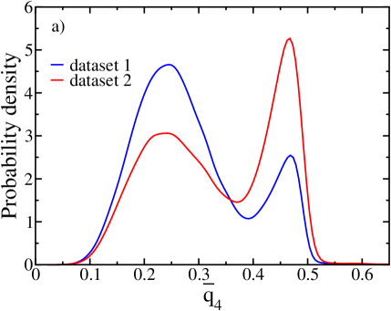
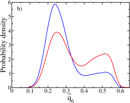
Figure 1: Probability densities of averaged local bond-order parameters $\overline{q}_{4}$ (a) and $\overline{q}_{6}$ (b) for dataset 1 (blue) and dataset 2 (red).

III Accuracy and performance

First, we compare the accuracy of our models by using the standard procedure, i.e., by computing the root mean square error (RMSE) for forces, energies, and in the case of the KbP also the stress tensor. We note that this sort of metric is sensitive to different factors. For example, a reduced RMSE does not necessarily indicate a universally superior model. If the database contains correlated data, the RMSE might decrease due to highly correlated data but this tells little about the stability of the MLFF. Consequently, one could obtain a smaller error even when the model is not reliable and robust. In essence, as the model has to tackle more of the relevant configurational space, the challenge increases, and the RMSE may rise despite the model becoming more robust. As explained above, we have produced two different datasets with varying sizes and data acquisition approaches. The differences in the RMSE of energy and forces of these sets are small, but nevertheless, we will see that stability issues appear later when observables are computed.

Table 2: Comparison of the accuracy of the KbP and BPNNP models trained on the highly accurate dataset 1 and on the on-the-fly dataset 2. The root mean square errors (RMSE) are given for (from left to right) energy (meV/atom), forces (meV/Å), and stress tensor (kbar).

method/software	dataset	ERMSE	FRMSE	SRMSE
	1	0.30	27	0.16
KbP/VASP	2	0.30	27	0.16
	1	0.26	28	-
BPNNP/n2p2	2	0.30	27	-

Results of this error analysis are shown in Table 2. The root mean square error in the KbP approach is $\sim$27 meV/Å in the force components, $\sim$0.30 meV/atom in the energy, and $\sim$0.16 kBar in the stress tensor for both data sets. As an additional test, we picked 40 configurations with 128 molecules from two KbP parallel tempering (PT) simulations (see Sec. IV.1). These span a temperature range from 210 to 330 K. For these structures, first-principles calculations were performed and compared to the KbP for the large training set. The average errors are in line with the 64 molecule training set error, e.g. 27 meV/Å for the force error, 0.2 meV/atom for energies, and 0.1 kbar (errors per atom and pressure errors decrease like one over the square root of the number of atoms, if there are no relevant long-range correlation effects). This suggests that finite-size errors related to the training set can be neglected.

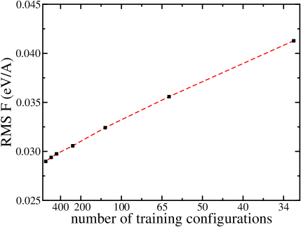
Figure 2: Learning curve for the KbP approach, trained on a subset of the large data set and evaluated on an independent test set (see text for details). As the error does not approach 0, log-log plots do not convey a concise message and therefore we chose a reciprocal representation for the $x$-axis. The error appears to be inversely proportional to the number of training structures.

In Fig. 2, learning curves are shown for the KbP. Here we have used subsets of the large training set, ranging from 32 structures up to the full dataset. The force errors were evaluated for the about 200 structures only present in the small data set (marked with “*” in Table 1). We see fairly fast convergence with respect to the number of training structures with diminishing improvements above about 500 structures. However, we also see that the learning curve levels off at about 28 meV/Å (the 200 test structures contain only a few ice-like structures and relatively more high-temperature structures than the training set).

Regarding the training of the Behler-Parrinello-Neural-Network (BPNNP) model, the network architecture consists of 2 hidden layers with 25 nodes each. Softplus is used as activation function and the RMSE as loss function. The cutoff is set to 6.36 Å. The symmetry functions are the same as in Morawietz at al. morawietz2016van leading to 2827 parameters (weights and biases) per BPNNP. We train and simulate our BPNNP with the n2p2 interface singraber2019parallel for LAMMPS thompson2022lammps . In particular, four different BPNNPs were trained on each of the two datasets. Again, we find negligible differences in the RMSE for forces and energies for a given dataset. However, small differences appear between the two sets. The first one results in better accuracy for the energy but it is slightly worse for the forces than the second. The tiny differences between the two datasets are not entirely surprising. The small difference between the BPNNP and KbP approach is, however, to some extent remarkable. As a matter of fact, both approaches are based on two- and three-body correlation functions and similar radial cutoffs. They also share a lack of explicit modeling of four-body correlations and long-range electrostatic effects.

At this point, we can conclude that the two approaches yield overall similar accuracy in the standard evaluation procedures. Since the BPNNP cannot learn the stress tensor whereas the KbP does, it is useful to predict the pressure for test structures using the BPNNP. The results are shown in Fig. 3. Clearly, the BPNNP is capable of providing a good pressure prediction through the learning of forces and energies without explicitly learning the stress tensor. Interestingly, when the training set data is not re-calculated at 2000 eV, that is, when we use the initial data at 1100 eV, the average deviation in pressure is about $-1$ kbar. The first-principles calculations however indicate a difference of $-0.75$ to $-0.85$ kBar between 1100 eV and 2000 eV. This discrepancy relates to the already mentioned issue that results are less robust and reliable if the original on-the-fly database is learned. We add here that during molecular dynamics simulations, VASP does not change the basis set. As the volume fluctuates, this causes slight changes in the effective plane wave cutoff, and this in turn slightly affects the energies and the stress tensor. This problem is eliminated by recalculating the entire database at the end. We emphasize that this problem is specific to molecular liquids, as we have never observed differences between learning the on-the-fly database or a recalculated database for solid-state systems.

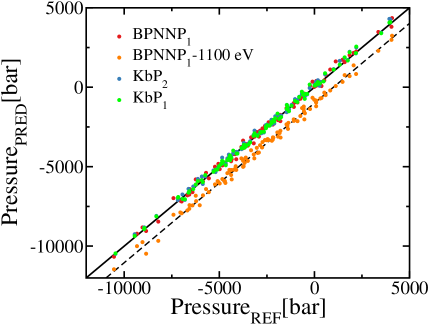
Figure 3: Predicted (PRED) vs. reference (REF) pressure for KbP, which learns the stress tensor, and BPNNP, which does not learn it. Also shown are results obtained with a BPNNP trained on a database without re-calculation at 2000 eV, i.e. trained on the original 1100 eV cutoff dataset. The offset in this case is $-1$ kbar, which is not in full agreement with the expected $\approx-0.8$ kbar. The coefficients (c₀, c₁) of the linear regression $y=c_{0}+c_{1}\cdot x$ are (0.051 kbar, 1.010) for BPNNP₁, ($-$1.00 kbar, 0.997) for BPNNP₁-1100 eV, (0.066 kbar, 1.007) for KbP₁, and (0.102 kbar, 1.007) for KbP₂.

Let us now assess the computational cost associated with each machine-learning method for the same computational resources. In both cases, the machine learning codes are optimized to run on CPUs. Specifically, we use a dual-socket AMD 7713 node (64 cores per socket). We cover system sizes from 384 atoms up to 384,000 atoms and run the simulations in the NVT ensemble. The summary of the computational cost is shown in Table 3. For VASP, we note that these calculations were performed in the kernel-based fast mode using ridge regression, forgoing Bayesian regression. No uncertainty predictions are possible in this mode, but the computational time is reduced by roughly a factor of 30. As can be seen in the table, the total run time (wall clock) is slightly lower for the BPNNP. We note that the KbP shows improved timings when reducing the number of cores for few atoms, whereas the BPNNP yields the best timings for the largest number of cores independently of the system size. We believe this is related to the huge bandwidth requirements for the evaluation of the kernels. VASP allows to sparsify the angular descriptors jinnouchi2020descriptors . This reduces the bandwidth requirements, improves the strong scaling, and is particularly beneficial for small systems, as shown by the numbers in parenthesis for KbP.

Table 3: Computational cost of energy and force prediction using a dual socket AMD 7713 node (64 core/socket). Smaller systems optimally require less cores for the KbP running VASP, whereas for the BPNNP running with n2p2 in LAMMPS using all cores provides better performance. Values in parentheses for KbP use only 30 % of the angular descriptors and 64 cores (128 cores for 24,576 and 384,000 atoms). Compute time depends to some extent on compilers, libraries, and MPI versions.

method/software	atoms	cores	$\mu$s/(atom$\cdot$step)
	384	128	9.2
	3,072	128	4.6
BPNNP/n2p2	24,576	128	4.1
	384,000	128	4.7
384	16	13.7 (3.8)
3,072	64	7.2 (4.6)
KbP/VASP	24,576	128	5.1 (4.2)
	384,000	128	5.3 (4.7)

We have also tested dataset 1 with the recent machine learning approach Allegro, a local equivariant deep neural network interatomic potentialmusaelian2023learning . A comparison of different methods is not straightforward in this case as Allegro is optimized to run on GPUs. Using a single Nvidia A100 GPU, an Allegro model with comparable accuracy to our models, unfortunately, requires 10 times longer than the 2 socket AMD nodes using KbP and BPNNP. In addition, Allegro can not yet predict the stress tensor and the use of NPT simulations is still under development. Therefore we have not included the Allegro model in further comparisons. Since better scaling with increasing GPU resources is expected for Allegro, the optimal ML approach for a given application may still depend on the available resources and the number of atoms in the simulation.

IV Physical properties

In this section, we apply both of our machine-learning potentials to obtain structural, thermodynamic, and dynamical properties of water with first-principles accuracy. We start by inspecting the density maximum and the melting temperature, followed by the partial radial distribution functions, and finally the self-diffusion coefficient. For compactness, we use the notation BPNNP₁ and KbP₁ for MLPs trained on the first larger dataset and BPNNP₂ and KbP₂ for MLPs trained on the second smaller on-the-fly dataset.

IV.1 Density maximum and melting temperature

To determine the density maximum of liquid water, we performed PT simulations for 128 molecules with temperatures ranging from 200 K up to 335 K at 1 bar. For all BPNNP, the duration of the simulations is 1 ns in each of the 32 replicas (2 million steps each). Four PT runs are launched for each of the four BPNNP that were trained for each of the two training sets. The first half of each trajectory is discarded as equilibration. In fact, we find that some lower-temperature replicas get kinetically trapped due to vitrification and stop to exchange Therefore, values for temperatures below 227 K are not shown in the plots. In the case of the KbP, we used only 20 replicas spanning a temperature range between 210 and 330 K. The spacing was roughly exponential. To make the simulations using the KbP more effective, the mass of hydrogen was increased to 8 a.m.u. and the timestep was set to 1.5 fs. Here only a single run was performed but using 10 million time steps giving a total simulation time of 15 ns for each replica. Additionally, a 7 ns parallel tempering run was performed for equilibration. As for training, Langevin thermostats were used for the atoms and the cell volume, but with a friction coefficient of 2 ps^-1. Likely because of the use of Langevin thermostats, we require longer simulation times to obtain good statistics in VASP.

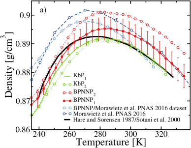
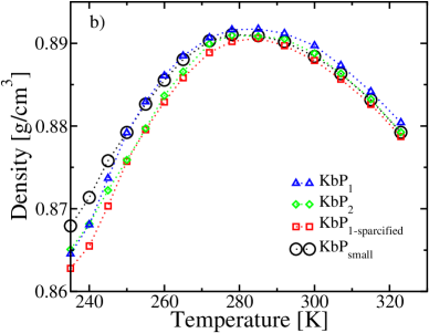
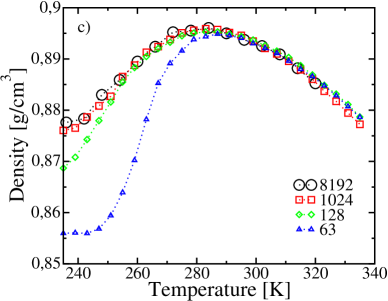
Figure 4: a) Density as a function of temperature at a pressure of 1 bar. The error bars for BPNNP₁ (solid red circles) are determined from the standard deviation over the four different BPNNP trained on dataset 1. For BPNNP₂ (empty red circles) only one run was stable and therefore no error bars are shown. KbP results are shown in green (solid for dataset 1 and empty for dataset 2); error bars for kbP₁ are determined using block averaging. The solid black line corresponds to experimental measurements hare1987density ; sotani2000volumetric ; holten2012thermodynamics and has been shifted down by 0.1075 g/cm³ to facilitate the comparison. Empty dark blue circles show results from Morawietz et al. morawietz2016van . Empty light blue circles correspond to the result of a parallel tempering simulation for a BPNNP trained here on the dataset of Morawietz et al. morawietz2016van . b) Comparison of various KbPs, including one trained only on 250 structures and one where the descriptors have been sparsified. c) Density versus temperature for different system sizes ranging from 63 to 8,192 molecules computed on the same BPNNP.

The results of these PT simulations are shown in Fig. 4. In the case of the BPNNP for the small second training set we encountered some issues: for three out of four trained potentials the simulations became unstable, and only for one, the four trajectories were completed without errors. Note that our RMSEs were almost the same as those for the BPNNP trained on the first, larger training set. This instability was never observed for the KbP trained on the same data, suggesting that BPNNPs require larger input data sets to become stable and robust. Moreover, we find an intrinsic error of about 1$\%$ in the density as obtained from the different runs on BPNNP as indicated by the error bars. This sort of uncertainty cannot be assessed for a KbP, because it is largely a deterministic approach. In any case, the difference between KbP₁ and KbP₂ which were trained on different datasets is very small.

Also shown in Fig. 4 are the results of Morawietz et al. morawietz2016van who used a BPNNP trained on data obtained using the same density functional but computed with FHI aims. This dataset was also refitted here, and parallel tempering simulations analogous to the other BPNNPs were performed. The difference to the original publication is about of the same order as the discrepancies between different BPNNPs fitted to the datasets generated in the present work. As can be seen in the figure, our results are in fairly good agreement with the previous results, for the present training data, however, the maximum is shifted to slightly higher temperatures. We find the density maximum for the RPBE+D3 functional at approximately 284 K using the BPNNP and 283 K using the KbP. We also compute the melting temperature. First, by running several trajectories for about 10 ns in the anisotropic NpT ensemble at standard pressure and different temperatures around the expected melting. Once, we find two consecutive temperatures in which ice barely grows or melts, we extract one of these configurations and continue the run in the NpH ensemble until the system converges to the melting temperature. For the BPNNP, the value obtained is 277 $\pm$ 1 K and for KbP 279 $\pm$ 1 K. Therefore, the difference between the melting and density maximum temperatures are 7 °C for the BPNNP and 4°C for the KbP, being in good agreement with experiments, where value for the temperature of maximum density is 4°C. Although the RPBE+D3 functional underestimates the density giving almost 10$\%$ smaller densities, the theoretical and experimental curves are very similar as shown in Fig. 4, where the experimental curve hare1987density ; sotani2000volumetric ; holten2012thermodynamics is shifted down by 0.1075 g/cm³. The shape of the maximum in the density is well reproduced.

Two more results for KbP are shown in Fig. 4 b) to assess whether further computational savings are possible without compromising quality. Both force fields result in force errors around 31 meV/Å, only slightly larger than for the other MLPs. The circles indicate results obtained using only 250 training structures from the large training set (compare also Fig. 2). Although the results are still very good, we see an increase in the density at low temperatures, which might be due to an insufficient number of training structures in the strongly supercooled regime. Furthermore, we report results for a KbP using only 30 % of the angular descriptors (compare Table 3), which speeds up the calculations by up to a factor of 2. Results are again in very good agreement with the other KbPs. Inspecting the four different curves for the KbP it is hard to make out systematic trends. It rather seems that these are similar in nature, but smaller than the variations for the BPNNPs, and hence a measure of the residual errors of the force fields. We note that the variations increase towards the supercooled liquid state, which might be related to a lack of training structures and thus increased uncertainty in that regime.

In the present work, we have also investigated how different system sizes affect the results. We have restricted this analysis to the BPNNPs, but expect similar results for the KbP. Figure 4 c) clearly indicates that 128 molecules are required to obtain technically converged results. Vitrification occurs very often in the smaller ensembles with 63 molecules. We also see that there are considerable system size dependencies below 250 K, where glassy states set in. This likely indicates that our data below 250 K should be considered with some caution and would require a more careful system size analysis, ideally with longer equilibration. Around the density maximum though the size effects are insignificant if at least 128 molecules are used.

IV.2 Radial distribution functions

Here, we compare the partial radial distribution functions (pRDF) for hydrogen-hydrogen (HH), oxygen-hydrogen (OH), and oxygen-oxygen (OO) at 300K. To do so, we run NpT simulations. In this case, the agreement between different MLPs is practically perfect, smaller than the line-width as can be seen in Fig. 5. Therefore, we decided to study the effect of temperature in the pRDF using only the KbP₁. The different pRDFs are depicted in Fig. 6, for 270 K, 300 K, 325 K, and 350 K. As expected, at lower temperatures water becomes more structured.

To conclude this section, we comment on the comparison to experimental results. Clearly, agreement between the present simulations and experiment is excellent, in particular, considering that quantum effects are disregarded in the present work. The inclusion of quantum effects would lower and broaden the first peak in the pRDF. It is not uncommon to approximate the effect of quantum effects by increasing the temperature: indeed the pRDFs at 325 K improve upon the already good agreement at 300 K.

Figure 5: Radial distribution functions for KbP₁ (dark-solid lines), KbP₂ (solid circles), and BPNNP₁ (light-dashed lines and circles) at 300K for the RPBE+D3 functional. Experimental results soper2013radial are shown in black. Hydrogen-hydrogen pRDFs are shown in blue a), oxygen-oxygen pRDFs in green b), and oxygen-hydrogen pRDFs in red c).

Figure 6: Effect of temperature on the partial radial distribution functions for a) hydrogen-hydrogen, b) oxygen-oxygen, and c) oxygen-hydrogen computed with the KbP.

IV.3 Self-diffusion coefficient

Finally, we compare the MLPs for the self-diffusion coefficient $D$. To make sure that the dynamics is not affected by the use of a thermostat, we equilibrated the system first in the NpT ensemble and then performed a production run in the NVE ensemble using 3,546 molecules and a simulation time of 0.5 ns (1 million timesteps). The same volume and starting structures were used for all MLPs. As usual, the diffusion coefficient is determined from the mean square displacement using the relation:

$$\langle|\vec{r}(t)-\vec{r}(0)|^{2}\rangle=6Dt.$$ (1)

Again, the agreement between the methods is excellent, in particular considering the statistical uncertainties. The KbP, based on the larger dataset yields slightly larger self-diffusion coefficients than the BPNNP based on the same dataset. Generally, the self-diffusion coefficients are slightly lower than those obtained by Morawietz et al. morawietz2016van and by Montero et al.montero2023kinetics . Over the available temperature range, agreement with experimentsgillen1972self ; holz2000temperature is also excellent.

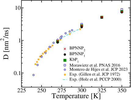
Figure 7: Self-diffusion coefficient $D$ as a function of temperature obtained from simulations with different MLPs. Also shown are experimental results.

V Discussion

In this work, we have compared two well-established machine-learning approaches that permit to transfer the accuracy of first-principles calculations to molecular simulations approaching the cost of simple force-field models. These approaches are the kernel-based method as implemented in VASP and the Behler-Parrinello neural network method implemented in n2p2. For the first principles calculations, we use RPBE+D3 with zero damping, which has previously been shown to reproduce fairly well both structural and dynamical properties of water. We have taken great care to make our first-principles dataset technically as accurate as possible: for instance, increasing the k-point density yields negligible (i.e., sub meV/Å) changes, and the cutoff was set to 2000 eV to minimize basis-set errors. Specifically, we emphasize that the use of a PW-cutoff of 1100 eV results in a Pulay stress error of about $-0.8$ kbar. This leads to an underestimation of the volume of about 5 % at zero pressure, which is hardly acceptable.

We prepared two distinct first-principles datasets. Both start out from 450 structures obtained from on-the-fly learning by melting cubic ice, equilibrating just below the boiling point, followed by several simulated annealing steps. The first set is extended by adding 1,000 structures from two parallel tempering runs covering the desired temperature range. The second set is based exclusively on on-the-fly learning adding 200 more structures generated again by simulated annealing. The first set is more diverse and expected to yield ”better” MLPs.

For the KbP approach, we find that the results do not depend very significantly on the chosen database. Pair correlation functions are practically indistinguishable for the two KpP. Slight differences are found for the isobars at low temperatures where vitrification occurs. This however has no noticeable impact on the liquid state and, in particular, on the density maximum. Results are less clear for the BPNNP. For the small training set, three out of four BPNNPs yield non-stable trajectories during parallel tempering, indicating that the neural network potentials require more training data and are more prone to instabilities when performing long simulations. For the large dataset, however, results from the BPNNP and the KbP simulations are very similar. Specifically, the radial distribution functions agree perfectly, within the line width of the shown plots. Also, there are no noteworthy differences in the self-diffusion coefficient. Furthermore, agreement with the experiment is very good for both BPNNP and KbP.

Despite the virtually perfect agreement for the pair correlation function and self-diffusion constant, slight but statistically significant differences are found for the density isobars. As mentioned, the KbP approach shows very consistent results for the two datasets as well as different settings. The BPNNPs show a more pronounced variation. When trained on the large dataset, we observe differences of about 1 % in the predicted densities for four different MLPs. Furthermore, the average density is about 0.5 % larger than for the KbP. The density maximum is also shifted slightly to higher temperatures. For the smaller training set — as mentioned, only one out of four BPNNPs was stable — the density for this single MLP was slightly higher than for the large database. It is not entirely trivial to explain this slight difference, but one possible explanation is that the BPNNP for technical reasons can not be trained on the pressure (to be precise the stress tensor). Recall that the pressure averaged over structures drawn from an NVT ensemble corresponds to the first derivative of the free energy. So if the pressure is not used for learning, potential errors for the equilibrium volume might be slightly larger. This in combination with the larger instability of the BPNNP potentials, might explain the slightly larger density that we obtain using BPNNPs. On the other hand, the predicted pressures using the BPNNP show no systematic error, so the previous arguments are not entirely conclusive. Unfortunately, we cannot even tell with certainty which of the two MLPs is more accurate. A full NPT first principles calculation at 2000 eV close to the density maximum is not feasible, as the dynamics of water is extremely slow. We estimate that at least 0.2 ns (100,000 steps) first principles calculations would be required to make sufficiently accurate predictions on the density of water to determine which potential yields a result closer to the RPBE+D3 ground truth. Also reweighting of MLP-created ensembles using first-principles calculations did not yield a conclusive result.

VI Summary and Conclusions

In summary, the differences between the different MLPs are, in fact, small. Specifically for the larger training dataset, the agreement between two entirely different MLPs is excellent, and no difference is noticeable for simple observables such as the diffusion constant or the pair-correlation function. The small discrepancies in the predicted density isobars are acceptable, at least for the large dataset. Recall that the difference in the density is only about 0.5 % which translates into a lattice constant difference of only about $0.15~{}\%$. Such a difference is negligible, if we consider that the errors introduced by approximate density functionals are usually considered to be at least $0.5~{}\%$ for lattice constants, but often reach 3 % for vdW or weakly interacting fragments. As a matter of fact, the density is underestimated by 10 % using RPBE+D3. The claim that the fitting errors are acceptable, is also supported by the observation that results obtained by fitting to an older dataset, based on the same density functional but computed with FHI AIMS, show a larger difference to the present work than the difference between the different MLPs fitted to the first-principles datasets obtained here. This indicates that the database is more relevant than how the database is fitted.

We finish with a word of caution. Root mean square errors for test datasets do not always convey the complete story. They are not indicative of stability, and even simple tests on say pair correlation functions might not be able to predict how large the differences might be for thermodynamic properties. It seems expedient to test at least two MLPs if some degree of certainty is desired, in particular, if it is not straightforward to simulate or check the observable using the full first-principles machinery.

VII Acknowledgments

The authors acknowledge the support from the SFB TACO (project nr. F81-N) funded by Austrian Science Fund FWF as well as the computer resources and technical assistance provided by the Vienna Scientific Cluster (VSC).

VIII Author declarations

VIII.1 Conflict of Interest

The authors have no conflicts to disclose.

References

- (1) J. Barker and R. Watts, “Structure of water; a monte carlo calculation,” Chemical Physics Letters, vol. 3, no. 3, pp. 144–145, 1969.
- (2) A. Rahman and F. H. Stillinger, “Molecular dynamics study of liquid water,” The Journal of Chemical Physics, vol. 55, no. 7, pp. 3336–3359, 1971.
- (3) K. Laasonen, F. Csajka, and M. Parrinello, “Water dimer properties in the gradient-corrected density functional theory,” Chemical Physics Letters, vol. 194, no. 3, pp. 172–174, 1992.
- (4) K. Laasonen, M. Sprik, M. Parrinello, and R. Car, ““ab initio”liquid water,” The Journal of Chemical Physics, vol. 99, no. 11, pp. 9080–9089, 1993.
- (5) M. Sprik, J. Hutter, and M. Parrinello, “Ab initio molecular dynamics simulation of liquid water: Comparison of three gradient-corrected density functionals,” The Journal of Chemical Physics, vol. 105, no. 3, pp. 1142–1152, 1996.
- (6) S. S. Xantheas, “Ab initio studies of cyclic water clusters (h2o) n, n= 1–6. iii. comparison of density functional with mp2 results,” The Journal of Chemical Physics, vol. 102, no. 11, pp. 4505–4517, 1995.
- (7) J. C. Grossman, E. Schwegler, E. W. Draeger, F. Gygi, and G. Galli, “Towards an assessment of the accuracy of density functional theory for first principles simulations of water,” The Journal of Chemical Physics, vol. 120, no. 1, pp. 300–311, 2004.
- (8) M. Chen, H.-Y. Ko, R. C. Remsing, M. F. Calegari Andrade, B. Santra, Z. Sun, A. Selloni, R. Car, M. L. Klein, J. P. Perdew, et al., “Ab initio theory and modeling of water,” Proceedings of the National Academy of Sciences, vol. 114, no. 41, pp. 10846–10851, 2017.
- (9) L. Ruiz Pestana, O. Marsalek, T. E. Markland, and T. Head-Gordon, “The quest for accurate liquid water properties from first principles,” The Journal of Physical Chemistry Letters, vol. 9, no. 17, pp. 5009–5016, 2018.
- (10) M. J. Gillan, D. Alfe, and A. Michaelides, “Perspective: How good is dft for water?,” The Journal of Chemical Physics, vol. 144, no. 13, 2016.
- (11) A. P. Gaiduk, F. Gygi, and G. Galli, “Density and compressibility of liquid water and ice from first-principles simulations with hybrid functionals,” The Journal of Physical Chemistry Letters, vol. 6, no. 15, pp. 2902–2908, 2015.
- (12) J. Schmidt, J. VandeVondele, I.-F. W. Kuo, D. Sebastiani, J. I. Siepmann, J. Hutter, and C. J. Mundy, “Isobaric- isothermal molecular dynamics simulations utilizing density functional theory: an assessment of the structure and density of water at near-ambient conditions,” The Journal of Physical Chemistry B, vol. 113, no. 35, pp. 11959–11964, 2009.
- (13) J. Wang, G. Román-Pérez, J. M. Soler, E. Artacho, and M.-V. Fernández-Serra, “Density, structure, and dynamics of water: The effect of van der waals interactions,” The Journal of Chemical Physics, vol. 134, no. 2, 2011.
- (14) G. Miceli, S. de Gironcoli, and A. Pasquarello, “Isobaric first-principles molecular dynamics of liquid water with nonlocal van der waals interactions,” The Journal of Chemical Physics, vol. 142, no. 3, 2015.
- (15) M. Ceriotti, J. Cuny, M. Parrinello, and D. E. Manolopoulos, “Nuclear quantum effects and hydrogen bond fluctuations in water,” Proceedings of the National Academy of Sciences, vol. 110, no. 39, pp. 15591–15596, 2013.
- (16) M. D. Baer, C. J. Mundy, M. J. McGrath, I.-F. W. Kuo, J. I. Siepmann, and D. J. Tobias, “Re-examining the properties of the aqueous vapor–liquid interface using dispersion corrected density functional theory,” The Journal of Chemical Physics, vol. 135, no. 12, 2011.
- (17) I.-C. Lin, A. P. Seitsonen, I. Tavernelli, and U. Rothlisberger, “Structure and dynamics of liquid water from ab initio molecular dynamics: Comparison of blyp, pbe, and revpbe density functionals with and without van der waals corrections,” Journal of Chemical Theory and Computation, vol. 8, no. 10, pp. 3902–3910, 2012.
- (18) J. VandeVondele, F. Mohamed, M. Krack, J. Hutter, M. Sprik, and M. Parrinello, “The influence of temperature and density functional models in ab initio molecular dynamics simulation of liquid water,” The Journal of Chemical Physics, vol. 122, no. 1, 2005.
- (19) L. Zheng, M. Chen, Z. Sun, H.-Y. Ko, B. Santra, P. Dhuvad, and X. Wu, “Structural, electronic, and dynamical properties of liquid water by ab initio molecular dynamics based on scan functional within the canonical ensemble,” The Journal of Chemical Physics, vol. 148, no. 16, 2018.
- (20) A. Zen, Y. Luo, G. Mazzola, L. Guidoni, and S. Sorella, “Ab initio molecular dynamics simulation of liquid water by quantum monte carlo,” The Journal of Chemical Physics, vol. 142, no. 14, 2015.
- (21) V. Molinero and E. B. Moore, “Water modeled as an intermediate element between carbon and silicon,” The Journal of Physical Chemistry B, vol. 113, no. 13, pp. 4008–4016, 2009.
- (22) K. M. Dyer, J. S. Perkyns, G. Stell, and B. Montgomery Pettitt, “Site-renormalised molecular fluid theory: on the utility of a two-site model of water,” Molecular Physics, vol. 107, no. 4-6, pp. 423–431, 2009.
- (23) W. L. Jorgensen, “Quantum and statistical mechanical studies of liquids. 10. transferable intermolecular potential functions for water, alcohols, and ethers. application to liquid water,” Journal of the American Chemical Society, vol. 103, no. 2, pp. 335–340, 1981.
- (24) H. J. Berendsen, J. P. Postma, W. F. van Gunsteren, and J. Hermans, “Interaction models for water in relation to protein hydration,” in Intermolecular forces: proceedings of the fourteenth Jerusalem symposium on quantum chemistry and biochemistry held in jerusalem, israel, april 13–16, 1981, pp. 331–342, Springer, 1981.
- (25) W. L. Jorgensen, J. Chandrasekhar, J. D. Madura, R. W. Impey, and M. L. Klein, “Comparison of simple potential functions for simulating liquid water,” The Journal of Chemical Physics, vol. 79, no. 2, pp. 926–935, 1983.
- (26) H. J. Berendsen, J. R. Grigera, and T. P. Straatsma, “The missing term in effective pair potentials,” Journal of Physical Chemistry, vol. 91, no. 24, pp. 6269–6271, 1987.
- (27) H. W. Horn, W. C. Swope, J. W. Pitera, J. D. Madura, T. J. Dick, G. L. Hura, and T. Head-Gordon, “Development of an improved four-site water model for biomolecular simulations: Tip4p-ew,” The Journal of Chemical Physics, vol. 120, no. 20, pp. 9665–9678, 2004.
- (28) J. Abascal, E. Sanz, R. García Fernández, and C. Vega, “A potential model for the study of ices and amorphous water: Tip4p/ice,” The Journal of Chemical Physics, vol. 122, no. 23, 2005.
- (29) J. L. Abascal and C. Vega, “A general purpose model for the condensed phases of water: Tip4p/2005,” The Journal of Chemical Physics, vol. 123, no. 23, 2005.
- (30) S. Izadi, R. Anandakrishnan, and A. V. Onufriev, “Building water models: a different approach,” The Journal of Physical Chemistry Letters, vol. 5, no. 21, pp. 3863–3871, 2014.
- (31) S. Piana, A. G. Donchev, P. Robustelli, and D. E. Shaw, “Water dispersion interactions strongly influence simulated structural properties of disordered protein states,” The Journal of Physical Chemistry B, vol. 119, no. 16, pp. 5113–5123, 2015.
- (32) M. A. González and J. L. Abascal, “A flexible model for water based on tip4p/2005,” The Journal of Chemical Physics, vol. 135, no. 22, 2011.
- (33) S. Habershon, T. E. Markland, and D. E. Manolopoulos, “Competing quantum effects in the dynamics of a flexible water model,” The Journal of Chemical Physics, vol. 131, no. 2, 2009.
- (34) F. H. Stillinger and A. Rahman, “Improved simulation of liquid water by molecular dynamics,” The Journal of Chemical Physics, vol. 60, no. 4, pp. 1545–1557, 1974.
- (35) M. W. Mahoney and W. L. Jorgensen, “A five-site model for liquid water and the reproduction of the density anomaly by rigid, nonpolarizable potential functions,” The Journal of Chemical Physics, vol. 112, no. 20, pp. 8910–8922, 2000.
- (36) S. W. Rick, “A reoptimization of the five-site water potential (tip5p) for use with ewald sums,” The Journal of Chemical Physics, vol. 120, no. 13, pp. 6085–6093, 2004.
- (37) H. Nada, “Anisotropy in geometrically rough structure of ice prismatic plane interface during growth: Development of a modified six-site model of h2o and a molecular dynamics simulation,” The Journal of Chemical Physics, vol. 145, no. 24, 2016.
- (38) S. Izadi and A. V. Onufriev, “Accuracy limit of rigid 3-point water models,” The Journal of Chemical Physics, vol. 145, no. 7, 2016.
- (39) L.-P. Wang, T. J. Martinez, and V. S. Pande, “Building force fields: An automatic, systematic, and reproducible approach,” The Journal of Physical Chemistry Letters, vol. 5, no. 11, pp. 1885–1891, 2014.
- (40) R. Fuentes-Azcatl and J. Alejandre, “Non-polarizable force field of water based on the dielectric constant: Tip4p/,” The Journal of Physical Chemistry B, vol. 118, no. 5, pp. 1263–1272, 2014.
- (41) P. T. Kiss and A. Baranyai, “A systematic development of a polarizable potential of water,” The Journal of Chemical Physics, vol. 138, no. 20, 2013.
- (42) J. Reimers, R. Watts, and M. Klein, “Intermolecular potential functions and the properties of water,” Chemical Physics, vol. 64, no. 1, pp. 95–114, 1982.
- (43) C. Tainter, P. A. Pieniazek, Y.-S. Lin, and J. L. Skinner, “Robust three-body water simulation model,” The Journal of Chemical Physics, vol. 134, no. 18, 2011.
- (44) H. Yu, T. Hansson, and W. F. van Gunsteren, “Development of a simple, self-consistent polarizable model for liquid water,” The Journal of Chemical Physics, vol. 118, no. 1, pp. 221–234, 2003.
- (45) G. S. Fanourgakis and S. S. Xantheas, “The flexible, polarizable, thole-type interaction potential for water (ttm2-f) revisited,” The Journal of Physical Chemistry A, vol. 110, no. 11, pp. 4100–4106, 2006.
- (46) H. Jiang, O. A. Moultos, I. G. Economou, and A. Z. Panagiotopoulos, “Hydrogen-bonding polarizable intermolecular potential model for water,” The Journal of Physical Chemistry B, vol. 120, no. 48, pp. 12358–12370, 2016.
- (47) E. R. Pinnick, S. Erramilli, and F. Wang, “Predicting the melting temperature of ice-ih with only electronic structure information as input,” The Journal of Chemical Physics, vol. 137, no. 1, 2012.
- (48) K. T. No, B. H. Chang, S. Y. Kim, M. S. Jhon, and H. A. Scheraga, “Description of the potential energy surface of the water dimer with an artificial neural network,” Chemical Physics Letters, vol. 271, no. 1-3, pp. 152–156, 1997.
- (49) J. Behler and M. Parrinello, “Generalized neural-network representation of high-dimensional potential-energy surfaces,” Physical Review Letters, vol. 98, no. 14, p. 146401, 2007.
- (50) T. Morawietz, V. Sharma, and J. Behler, “A neural network potential-energy surface for the water dimer based on environment-dependent atomic energies and charges,” The Journal of Chemical Physics, vol. 136, no. 6, 2012.
- (51) T. Morawietz, A. Singraber, C. Dellago, and J. Behler, “How van der waals interactions determine the unique properties of water,” Proceedings of the National Academy of Sciences, vol. 113, no. 30, pp. 8368–8373, 2016.
- (52) A. Singraber, T. Morawietz, J. Behler, and C. Dellago, “Density anomaly of water at negative pressures from first principles,” Journal of Physics: Condensed Matter, vol. 30, no. 25, p. 254005, 2018.
- (53) P. Montero de Hijes, S. Romano, A. Gorfer, and C. Dellago, “The kinetics of the ice–water interface from ab initio machine learning simulations,” The Journal of Chemical Physics, vol. 158, no. 20, 2023.
- (54) B. Cheng, J. Behler, and M. Ceriotti, “Nuclear quantum effects in water at the triple point: Using theory as a link between experiments,” The Journal of Physical Chemistry Letters, vol. 7, no. 12, pp. 2210–2215, 2016.
- (55) V. Kapil, J. Behler, and M. Ceriotti, “High order path integrals made easy,” The Journal of Chemical Physics, vol. 145, no. 23, 2016.
- (56) V. Kapil, D. M. Wilkins, J. Lan, and M. Ceriotti, “Inexpensive modeling of quantum dynamics using path integral generalized langevin equation thermostats,” The Journal of Chemical Physics, vol. 152, no. 12, 2020.
- (57) B. Cheng, E. A. Engel, J. Behler, C. Dellago, and M. Ceriotti, “Ab initio thermodynamics of liquid and solid water,” Proceedings of the National Academy of Sciences, vol. 116, no. 4, pp. 1110–1115, 2019.
- (58) T. Morawietz, O. Marsalek, S. R. Pattenaude, L. M. Streacker, D. Ben-Amotz, and T. E. Markland, “The interplay of structure and dynamics in the raman spectrum of liquid water over the full frequency and temperature range,” The Journal of Physical Chemistry Letters, vol. 9, no. 4, pp. 851–857, 2018.
- (59) A. Reinhardt and B. Cheng, “Quantum-mechanical exploration of the phase diagram of water,” Nature Communications, vol. 12, no. 1, p. 588, 2021.
- (60) B. Cheng, M. Bethkenhagen, C. J. Pickard, and S. Hamel, “Phase behaviours of superionic water at planetary conditions,” Nature Physics, vol. 17, no. 11, pp. 1228–1232, 2021.
- (61) O. Wohlfahrt, C. Dellago, and M. Sega, “Ab initio structure and thermodynamics of the rpbe-d3 water/vapor interface by neural-network molecular dynamics,” The Journal of Chemical Physics, vol. 153, no. 14, 2020.
- (62) B. J. Braams and J. M. Bowman, “Permutationally invariant potential energy surfaces in high dimensionality,” International Reviews in Physical Chemistry, vol. 28, no. 4, pp. 577–606, 2009.
- (63) Q. Yu, C. Qu, P. L. Houston, R. Conte, A. Nandi, and J. M. Bowman, “q-aqua: A many-body ccsd (t) water potential, including four-body interactions, demonstrates the quantum nature of water from clusters to the liquid phase,” The Journal of Physical Chemistry Letters, vol. 13, no. 22, pp. 5068–5074, 2022.
- (64) X. Zhu, M. Riera, E. F. Bull-Vulpe, and F. Paesani, “Mb-pol (2023): Sub-chemical accuracy for water simulations from the gas to the liquid phase,” Journal of Chemical Theory and Computation, 2023.
- (65) A. P. Bartók, M. J. Gillan, F. R. Manby, and G. Csányi, “Machine-learning approach for one-and two-body corrections to density functional theory: Applications to molecular and condensed water,” Physical Review B, vol. 88, no. 5, p. 054104, 2013.
- (66) S. Bose, D. Dhawan, S. Nandi, R. R. Sarkar, and D. Ghosh, “Machine learning prediction of interaction energies in rigid water clusters,” Physical Chemistry Chemical Physics, vol. 20, no. 35, pp. 22987–22996, 2018.
- (67) L. Zhang, H. Wang, R. Car, and E. Weinan, “Phase diagram of a deep potential water model,” Physical Review Letters, vol. 126, no. 23, p. 236001, 2021.
- (68) A. Torres, L. S. Pedroza, M. Fernandez-Serra, and A. R. Rocha, “Using neural network force fields to ascertain the quality of ab initio simulations of liquid water,” The Journal of Physical Chemistry B, vol. 125, no. 38, pp. 10772–10778, 2021.
- (69) D. Lu, H. Wang, M. Chen, L. Lin, R. Car, E. Weinan, W. Jia, and L. Zhang, “86 pflops deep potential molecular dynamics simulation of 100 million atoms with ab initio accuracy,” Computer Physics Communications, vol. 259, p. 107624, 2021.
- (70) D. Tisi, L. Zhang, R. Bertossa, H. Wang, R. Car, and S. Baroni, “Heat transport in liquid water from first-principles and deep neural network simulations,” Physical Review B, vol. 104, no. 22, p. 224202, 2021.
- (71) K. Xu, Y. Hao, T. Liang, P. Ying, J. Xu, J. Wu, and Z. Fan, “Accurate prediction of heat conductivity of water by a neuroevolution potential,” The Journal of Chemical Physics, vol. 158, no. 20, 2023.
- (72) C. Malosso, L. Zhang, R. Car, S. Baroni, and D. Tisi, “Viscosity in water from first-principles and deep-neural-network simulations,” npj Computational Materials, vol. 8, no. 1, p. 139, 2022.
- (73) J. Xu, C. Zhang, L. Zhang, M. Chen, B. Santra, and X. Wu, “Isotope effects in molecular structures and electronic properties of liquid water via deep potential molecular dynamics based on the scan functional,” Physical Review B, vol. 102, no. 21, p. 214113, 2020.
- (74) T. E. Gartner III, L. Zhang, P. M. Piaggi, R. Car, A. Z. Panagiotopoulos, and P. G. Debenedetti, “Signatures of a liquid–liquid transition in an ab initio deep neural network model for water,” Proceedings of the National Academy of Sciences, vol. 117, no. 42, pp. 26040–26046, 2020.
- (75) T. E. Gartner III, P. M. Piaggi, R. Car, A. Z. Panagiotopoulos, and P. G. Debenedetti, “Liquid-liquid transition in water from first principles,” Physical Review Letters, vol. 129, no. 25, p. 255702, 2022.
- (76) P. M. Piaggi, J. Weis, A. Z. Panagiotopoulos, P. G. Debenedetti, and R. Car, “Homogeneous ice nucleation in an ab initio machine-learning model of water,” Proceedings of the National Academy of Sciences, vol. 119, no. 33, p. e2207294119, 2022.
- (77) V. Zaverkin, D. Holzmüller, R. Schuldt, and J. Kästner, “Predicting properties of periodic systems from cluster data: A case study of liquid water,” The Journal of Chemical Physics, vol. 156, p. 114103, 2022.
- (78) S. Batzner, A. Musaelian, L. Sun, M. Geiger, J. P. Mailoa, M. Kornbluth, N. Molinari, T. E. Smidt, and B. Kozinsky, “E (3)-equivariant graph neural networks for data-efficient and accurate interatomic potentials,” Nature Communications, vol. 13, no. 1, p. 2453, 2022.
- (79) A. Musaelian, S. Batzner, A. Johansson, L. Sun, C. J. Owen, M. Kornbluth, and B. Kozinsky, “Learning local equivariant representations for large-scale atomistic dynamics,” Nature Communications, vol. 14, no. 1, p. 579, 2023.
- (80) D. P. Kovács, I. Batatia, E. S. Arany, and G. Csányi, “Evaluation of the MACE force field architecture: From medicinal chemistry to materials science,” The Journal of Chemical Physics, vol. 159, p. 044118, 07 2023.
- (81) X. Fu, Z. Wu, W. Wang, T. Xie, S. Keten, R. Gomez-Bombarelli, and T. Jaakkola, “Forces are not enough: Benchmark and critical evaluation for machine learning force fields with molecular simulations,” arXiv preprint arXiv:2210.07237, 2022.
- (82) T. T. Nguyen, E. Székely, G. Imbalzano, J. Behler, G. Csányi, M. Ceriotti, A. W. Götz, and F. Paesani, “Comparison of permutationally invariant polynomials, neural networks, and gaussian approximation potentials in representing water interactions through many-body expansions,” The Journal of Chemical Physics, vol. 148, no. 24, 2018.
- (83) G. Kresse and J. Furthmüller, “Efficient iterative schemes for ab initio total-energy calculations using a plane-wave basis set,” Physical review B, vol. 54, no. 16, p. 11169, 1996.
- (84) G. Kresse and J. Furthmüller, “Efficiency of ab-initio total energy calculations for metals and semiconductors using a plane-wave basis set,” Computational materials science, vol. 6, no. 1, pp. 15–50, 1996.
- (85) R. Jinnouchi, J. Lahnsteiner, F. Karsai, G. Kresse, and M. Bokdam, “Phase transitions of hybrid perovskites simulated by machine-learning force fields trained on the fly with bayesian inference,” Physical Review Letters, vol. 122, no. 22, p. 225701, 2019.
- (86) R. Jinnouchi, F. Karsai, and G. Kresse, “On-the-fly machine learning force field generation: Application to melting points,” Physical Review B, vol. 100, no. 1, p. 014105, 2019.
- (87) R. Jinnouchi, F. Karsai, C. Verdi, R. Asahi, and G. Kresse, “Descriptors representing two-and three-body atomic distributions and their effects on the accuracy of machine-learned inter-atomic potentials,” The Journal of Chemical Physics, vol. 152, no. 23, 2020.
- (88) P. E. Blöchl, “Projector augmented-wave method,” Physical review B, vol. 50, no. 24, p. 17953, 1994.
- (89) G. Kresse and D. Joubert, “From ultrasoft pseudopotentials to the projector augmented-wave method,” Physical review b, vol. 59, no. 3, p. 1758, 1999.
- (90) B. Hammer, L. B. Hansen, and J. K. Nørskov, “Improved adsorption energetics within density-functional theory using revised perdew-burke-ernzerhof functionals,” Physical review B, vol. 59, no. 11, p. 7413, 1999.
- (91) S. Grimme, J. Antony, S. Ehrlich, and H. Krieg, “A consistent and accurate ab initio parametrization of density functional dispersion correction (dft-d) for the 94 elements h-pu,” The Journal of Chemical Physics, vol. 132, no. 15, 2010.
- (92) R. Jinnouchi, S. Minami, F. Karsai, C. Verdi, and G. Kresse, “Proton transport in perfluorinated ionomer simulated by machine-learned interatomic potential,” The Journal of Physical Chemistry Letters, vol. 14, no. 14, pp. 3581–3588, 2023.
- (93) H. Wang and W. Yang, “Force field for water based on neural network,” The Journal of Physical Chemistry Letters, vol. 9, pp. 3232–3240, 2018.
- (94) L. Yang, J. Li, F. Chen, and K. Yu, “A transferrable range-separated force field for water: Combining the power of both physically-motivated models and machine learning techniques,” The Journal of Chemical Physics, vol. 157, no. 21, 2022.
- (95) W. Lechner and C. Dellago, “Accurate determination of crystal structures based on averaged local bond order parameters,” The Journal of Chemical Physics, vol. 129, no. 11, 2008.
- (96) E. Sanz, C. Vega, J. Espinosa, R. Caballero-Bernal, J. Abascal, and C. Valeriani, “Homogeneous ice nucleation at moderate supercooling from molecular simulation,” Journal of the American Chemical Society, vol. 135, no. 40, pp. 15008–15017, 2013.
- (97) B. Monserrat, J. G. Brandenburg, E. A. Engel, and B. Cheng, “Liquid water contains the building blocks of diverse ice phases,” Nature Communications, vol. 11, no. 1, p. 5757, 2020.
- (98) F. Guidarelli Mattioli, F. Sciortino, and J. Russo, “Are neural network potentials trained on liquid states transferable to crystal nucleation? a test on ice nucleation in the mw water model,” The Journal of Physical Chemistry B, vol. 127, no. 17, pp. 3894–3901, 2023.
- (99) A. Singraber, T. Morawietz, J. Behler, and C. Dellago, “Parallel multistream training of high-dimensional neural network potentials,” Journal of Chemical Theory and Computation, vol. 15, no. 5, pp. 3075–3092, 2019.
- (100) A. P. Thompson, H. M. Aktulga, R. Berger, D. S. Bolintineanu, W. M. Brown, P. S. Crozier, P. J. in’t Veld, A. Kohlmeyer, S. G. Moore, T. D. Nguyen, et al., “Lammps-a flexible simulation tool for particle-based materials modeling at the atomic, meso, and continuum scales,” Computer Physics Communications, vol. 271, p. 108171, 2022.
- (101) D. Hare and C. Sorensen, “The density of supercooled water. ii. bulk samples cooled to the homogeneous nucleation limit,” The Journal of Chemical Physics, vol. 87, no. 8, pp. 4840–4845, 1987.
- (102) T. Sotani, J. Arabas, H. Kubota, M. Kijima, and S. Asada, “Volumetric behaviour of water under high pressure at subzero temperature,” HIGH TEMPERATURES HIGH PRESSURES, vol. 32, no. 4, pp. 433–440, 2000.
- (103) V. Holten, C. Bertrand, M. Anisimov, and J. Sengers, “Thermodynamics of supercooled water,” The Journal of Chemical Physics, vol. 136, no. 9, 2012.
- (104) A. K. Soper, “The radial distribution functions of water as derived from radiation total scattering experiments: Is there anything we can say for sure?,” International Scholarly Research Notices, vol. 2013, 2013.
- (105) K. T. Gillen, D. Douglass, and M. Hoch, “Self-diffusion in liquid water to- 31 c,” The Journal of Chemical Physics, vol. 57, no. 12, pp. 5117–5119, 1972.
- (106) M. Holz, S. R. Heil, and A. Sacco, “Temperature-dependent self-diffusion coefficients of water and six selected molecular liquids for calibration in accurate 1h nmr pfg measurements,” Physical Chemistry Chemical Physics, vol. 2, no. 20, pp. 4740–4742, 2000.