Anisotropic cold plasma modes in the chiral vector MCFJ electrodynamics

Abstract

In this work, we study the propagation and absorption of plasma waves in the context of the Maxwell-Carroll-Field-Jackiw (MCFJ) electrodynamics, with a purely spacelike background playing the role of the anomalous Hall conductivity. The Maxwell equations are rewritten for a cold, uniform and collisionless fluid plasma model, allowing us to determine the new refractive indices and propagating modes. The analysis begins for the propagation along the magnetic axis, being examined the cases of chiral vector parallel and orthogonal to the magnetic field. Two distinct refractive indices (associated with RCP and LCP waves) are attained, with the associated propagation and absorption zones determines. The low frequency regime is discussed, with the attainment of RCP and LCP helicons. Optical effects, as birefringence and dichroism, are scrutinized, being observed rotatory power sign reversion, a property of chiral MCFJ plasmas. The case of transversal propagation to the direction orthogonal of the magnetic field is also examined, providing much more involved results.

I Introduction

The propagation properties of electromagnetic waves in a cold magnetized plasma was based on the standard Maxwell equations to describe radio wave propagation in the ionosphere [1, 2, 3, 4, 5, 6]. The interaction of electromagnetic waves and atmosphere has attracted the attention of researchers over the years, including new investigations on reflection, absorption, and transmission in in topical plasma cenarios [7]. The cold plasma limit is adopted to study the fluid plasma behavior under the action of a constant external magnetic field [8, 9, 11, 10, 12, 13], being defined when the excitation energies are small, so that the thermal and collisional effects can be neglected. In this regime, the ions can be taken as infinitely massive, in such a way they do not answer to electromagnetic oscillations, especially to high-frequency waves. The cold plasma behavior is then described considering first-order differential equations written for the electron number density, $n$, and the electron fluid velocity, $\mathbf{u}$, namely

$$\frac{\partial n}{\partial t}+\mathbf{\nabla}\cdot\left(n\mathbf{u}\right)=0,$$ (1)

$$\frac{\partial\mathbf{u}}{\partial t}+\mathbf{u}\cdot\mathbf{\nabla u}=\frac{q}{m}\left(\mathbf{E}+\mathbf{u}\times\mathbf{B}_{0}\right),$$ (2)

where $\mathbf{B}_{0}$ represents the average magnetic field, $q$ and $m$ stand for the (electron) charge and mass. The linearized version of the magnetized cold plasmas considers fluctuations around average quantities, $n_{0}$ and $\mathbf{B}_{0}$, which are constant in space and time. Following the usual procedure, assuming $\mathbf{B}_{0}=B_{0}\hat{z}$, the corresponding plasma dielectric tensor is

$$\varepsilon_{ij}(\omega)=\varepsilon_{0}\begin{bmatrix}S&-iD&0\\ iD&S&0\\ 0&0&P\end{bmatrix},$$ (3)

where $\varepsilon_{0}$ is the vacuum electric permittivity, and

$$S=1-\frac{\omega_{p}^{2}}{\left(\omega^{2}-\omega_{c}^{2}\right)},\ D=\frac{\omega_{c}\omega_{p}^{2}}{\omega\left(\omega^{2}-\omega_{c}^{2}\right)},\ P=1-\frac{\omega_{p}^{2}}{\omega^{2}},$$ (4)

with $\omega_{p}=n_{0}q^{2}/(m\epsilon_{0})$, $\omega_{c}=|q|B_{0}/m$ being the plasma and cyclotron frequencies, respectively.

From the Maxwell theory, two distinct refractive indices are obtained for longitudinal propagation to the magnetic field, $\mathbf{k}\parallel\mathbf{B}_{0}$,

$$n_{\pm}=\sqrt{1-\frac{\omega_{p}^{2}}{\omega\left(\omega\pm\omega_{c}\right)}},$$ (5)

which provide right-handed circularly polarized (RCP) and left-handed circularly polarized (LCP) modes [1].

This is the standard result of wave propagation in the usual magnetized cold plasma. The refractive indices (5) present the following cutoff frequencies $\omega_{\pm}$:

$$\omega_{\pm} =\frac{1}{2}\left(\sqrt{\omega_{c}^{2}+4\omega_{p}^{2}}\mp\omega_{c}\right),$$ (6)

which define limits of the propagation and absorption zones. For propagation orthogonal to the magnetic field, $\mathbf{k}\perp\mathbf{B}_{0}$, $\mathbf{k}=(k_{x},k_{y},0)$, it is found that the corresponding transversal mode, $\delta\mathbf{E}=(0,0,\delta E_{z})$, is associated with the refractive index

$$n_{T}=\sqrt{1-\frac{\omega_{p}^{2}}{\omega^{2}}},$$ (7)

while the extraordinary longitudinal mode, $\delta\mathbf{E}=(\delta E_{x},\delta E_{y},0)$ is related to [13],

$$n_{O}=\sqrt{\frac{\left(S+D\right)\left(S-D\right)}{S}},$$ (8)

with $P$, $S$ and $D$ given in Eq. (4). The refractive index $n_{T}$ provides a linearly polarized propagating mode, whereas $n_{O}$, in general, is related to an elliptically polarized mode.

In condensed matter systems, chiral media are endowed with optical activity [14] stemming from parity-odd models, as bi-isotropic [15] and bi-anisotropic electrodynamics [16, 17, 18, 19, 20, 21], where circularly polarized waves propagate at distinct phase velocities, yielding birefringence and optical rotation [22]. Such an optical activity is due anisotropies of the matter structure or can be implied by external fields (Faraday effect [23, 24, 25]), being measured in terms of rotatory power (RP) [26]. Magneto-optical effects constitute a useful tool to investigate new materials, such as topological insulators [27, 28, 29, 30, 31, 32, 33] and graphene compounds [34].

In the context of modified electrodynamics, the Maxwell-Carroll-Field-Jackiw (MCFJ) electrodynamics was initially proposed to examine the possibility of CPT and Lorentz violation (LV) in free space, establishing severe constraints on the magnitude of the LV coefficients [35]. This model also represents the CPT-odd piece of the U(1) gauge sector of the broad Standard Model Extension (SME) [36]. The SME has been extensively examined by many authors, in a variety of scenarios, for instance, in radiative evaluations [37, 38], topological defects solutions [39], supersymmetry [40], and classical and quantum aspects [41]. The MCFJ electrodynamics is also relevant due to its connection with the axion Lagrangian [42, 43],

$$\mathrm{{\mathcal{L}}}=-\frac{1}{4}F^{\mu\nu}F_{\mu\nu}+\theta(\mathbf{E}\cdot\mathbf{B)},$$ (9)

where $F_{\mu\nu}=\partial_{\mu}A_{\nu}-\partial_{\nu}A_{\mu}$ is the field strength and the axion term, $\theta\,\tilde{F}^{\alpha\beta}F_{\alpha\beta}$, implies

$$\mathrm{{\mathcal{L}}}=-\frac{1}{4}F^{\mu\nu}F_{\mu\nu}+\frac{1}{4}\epsilon^{\mu\nu\alpha\beta}\left(\partial_{\mu}\theta\right)A_{\nu}F_{\alpha\beta}.$$ (10)

with the dual tensor, $\tilde{F}^{\mu\nu}=(1/2)\epsilon^{\mu\nu\alpha\beta}F_{\alpha\beta}$. In the case the axion derivative is a constant vector, $\partial_{\mu}\theta=(k_{AF})_{\mu}$, Lagrangian (10) recovers the MCFJ one,

$$\mathrm{{\mathcal{L}}}=-\frac{1}{4}G^{\mu\nu}F_{\mu\nu}+\frac{1}{4}\epsilon^{\mu\nu\alpha\beta}\left(k_{AF}\right)_{\mu}A_{\nu}F_{\alpha\beta}-A_{\mu}J^{\mu},$$ (11)

with $\left(k_{AF}\right)_{\mu}$ being the LV 4-vector background and $G^{\mu\nu}=\frac{1}{2}\chi^{\mu\nu\alpha\beta}F_{\alpha\beta}$ the continuous matter field strength. Such a Lagrangian provides the modified electrodynamics in matter, described by the inhomogeneous Maxwell equations,

$$\nabla\cdot\mathbf{D} =J^{0}-\mathbf{k}_{AF}\cdot\mathbf{B},$$ (12)

$$\nabla\times\mathbf{H}-\frac{\partial\mathbf{D}}{\partial t} =\mathbf{J}-k_{AF}^{0}\mathbf{B}+\mathbf{k}_{AF}\times\mathbf{E},$$ (13)

where $G^{i0}=D^{i}$, $G^{ij}=-\epsilon_{ijk}H^{k}$, and $\quad(k_{AF})^{\mu}=(k_{AF}^{0},\mathbf{k}_{AF})$. These must be considered together with the homogeneous Maxwell equations, obtained from the Bianchi identity $\partial_{\mu}\tilde{F}^{\mu\nu}=0$, and suitable constitutive relations.

The timelike CFJ component, $k_{AF}^{0}$, appears in the modified Ampère’s law (13) composing the chiral magnetic current, $\mathbf{J}_{B}=k_{AF}^{0}\mathbf{B}$, which has been used to investigate electromagnetic properties of matter endowed with the Chiral Magnetic Effect (CME) [44]. The CME [45, 46] consists of a macroscopic linear magnetic current law, ${\bf J}={\sigma}_{B}{\bf B}$, stemming from an asymmetry between the number density of left- and right-handed chiral fermions. Such an effect has been much investigated in a plethora of distinct contexts [48, 47, 49, 52, 50, 51, 52], including Weyl semimetals (WSMs) [53], where the chiral current may be different from the usual CME linear relation when electric and magnetic fields are applied, yielding a current effectively proportional to $B^{2}$, that is, ${\bf J}={\sigma}({\bf E}\cdot{\bf B}){\bf B}$ [31, 55, 54].

The spacelike vector, $\mathbf{k}_{AF}$, describes an anomalous charge density in the Gauss’s law (12) and contributes to the current density, $\mathbf{J}_{AH}=\mathbf{k}_{AF}\times\mathbf{E}$, in the Ampère’s law (13), associated to the anomalous Hall effect (AHE), with $\mathbf{k}_{AF}$ playing the role of anomalous Hall conductivity [44]. The AHE engenders an electric current in the presence of an electric field, due to the separation between the energy-crossing points in momentum space for right-handed and left-handed fermions [57, 58, 59, 56]. It has been investigated in distinct contexts, such as non-collinear antiferromagnets [60, 61], chiral spin-liquids [62], and WSMs [63]. Optical effects of a WSM with broken time-reversal and inversion symmetries governed by the axion and the AHE terms were recently examined in WSM systems, with focus on magneto-optical (Faraday, Kerr, and Voigt) effects [63, 64]. The AHE term has also been considered in the propagation of surface plasmon polaritons in WSMs [65]. Optical effects induced by the current term $\mathbf{k}_{AF}\times\mathbf{E}$ were also examined in the context of the MCFJ electrodynamics in continuous media [66].

In a recent investigation [67], the chiral effects of the CFJ timelike (pseudoscalar) chiral component, $k_{AF}^{0}$, on the electromagnetic modes in magnetized cold plasmas have been addressed. The electromagnetic and optical properties of the propagating modes, such as birefringence, absorption, and optical rotation have been discussed, with careful comparisons with the usual cold plasma features allowing the identification of the role played by the chiral factor.

In this work, we study wave propagation in a magnetized cold plasma governed by the Maxwell equations (12) and (13) modified by the AHE current term, $\mathbf{J}_{AH}=\mathbf{k}_{AF}\times\mathbf{E}$, which, using plane wave ansatz, read

$$i\varepsilon_{ij}{k^{i}}{{E^{j}}}+\mathbf{k}_{AF}\cdot\mathbf{{B}} =0,$$ (14a)

$$i\mathbf{k}\times\mathbf{{B}}+i\mu_{0}\omega\varepsilon_{ij}{k^{i}}{{E^{j}}}-\mu_{0}\mathbf{k}_{AF}\times\mathbf{{E}} =0.$$ (14b)

We also consider anisotropic constitutive relations (in the electric polarization sector),

$$D^{i}=\varepsilon_{ij}(\omega)E^{j},\ \ \ B^{i}=\mu_{0}H^{i}.$$ (15)

where $\varepsilon_{ij}$ is the cold plasma permittivity Eq. (3) and $\mu_{0}$ is the vacuum permeability. The modified wave equation for the electric field,

$$M_{ij}{E}^{j}=0,$$ (16)

with

$$M_{ij}=n^{2}\delta_{ij}-n_{i}n_{j}-\frac{\varepsilon_{ij}}{\varepsilon_{0}}-\frac{i}{\omega}\epsilon_{ikj}V^{k},$$ (17)

written in terms of the refractive index, $\mathbf{n}=\mathbf{k}/\omega$, and $V^{k}=k_{AF}^{k}/\varepsilon_{0}$ appearing as the redefined components of the chiral vector (which breaks the time-reversal symmetry and preserves space inversion). In this scenario, the wave equation (16) becomes

$$\left[n^{2}\delta_{ij}-n^{i}n^{j}-\frac{{\varepsilon}_{ij}}{\varepsilon_{0}}-i\frac{V^{k}}{\omega}\epsilon_{ikj}\right]{E}^{j}=0,$$ (18)

from which arise the dispersion relations that describe the wave propagation in the medium (by setting $\det M_{ij}=0$). To obtain the electromagnetic collective modes of a cold plasma modified by the anomalous Hall current-like term, one implements the plasma permittivity tensor (3) in the wave equation (18), yielding the linear homogeneous system,

$$\begin{bmatrix}n^{2}-n_{x}^{2}-S&-n_{x}n_{y}+iD+i\left(V_{z}/\omega\right)&-n_{x}n_{z}-i\left(V_{y}/\omega\right)\\ -n_{x}n_{y}-iD-i\left(V_{z}/\omega\right)&n^{2}-n_{y}^{2}-S&-n_{y}n_{z}+i\left(V_{x}/\omega\right)\\ -n_{x}n_{z}+i\left(V_{y}/\omega\right)&-n_{y}n_{z}-i\left(V_{x}/\omega\right)&n^{2}-n^{2}_{z}-P\end{bmatrix}\begin{bmatrix}\delta E_{x}\\ \delta E_{y}\\ \delta E_{z}\end{bmatrix}=0.$$ (19)

The refractive indices and associated propagating modes are also obtained, allowing the examination of the optical effects of birefringence and dichroism. Each scenario will be analyzed in the cases of propagation along the magnetic field and orthogonal to the magnetic field, also known as Faraday and Voigt configurations, respectively [68].

This paper is outlined as follows. In Sec. II, we obtain the general dispersion relation for a cold magnetized plasma in the presence of the anomalous Hall current, considering Faraday configuration. In Sec. III, we discuss the general properties of the cold plasma modes in the Voigt configuration. The dispersion relations, refractive indices, and optical properties, such as birefringence and absorption, are carried out in all cases examined. Finally, we summarize our results in Sec. IV.

II Wave propagation along the magnetic field axis

In this section, we analyze the wave propagation along the magnetic field direction, that is, $\mathbf{n}=n\hat{z}$. Then it holds

$$\begin{bmatrix}n^{2}-S&+iD+i\left(\left|\mathbf{V}\right|/\omega\right)\cos\beta&-i\left(\lvert\mathbf{V}\rvert/\omega\right)\sin\phi\sin\beta\\ -iD-i\left(\left|\mathbf{V}\right|/\omega\right)\cos\beta&n^{2}-S&+i\left(\left|\mathbf{V}\right|/\omega\right)\sin\beta\cos\phi\\ i\left(\lvert\mathbf{V}\rvert/\omega\right)\sin\phi\sin\beta&-i\left(\left|\mathbf{V}\right|/\omega\right)\sin\beta\cos\phi&-P\end{bmatrix}\begin{bmatrix}\delta E_{x}\\ \delta E_{y}\\ \delta E_{z}\end{bmatrix}=0\,,$$ (20)

where we have used, without loss of generality, the spherical parametrization

$$\mathbf{V}=\lvert\mathbf{V}\rvert\left(\sin\beta\cos\phi,\sin\beta\sin\phi,\cos\beta\right),$$ (21)

with the angle $\beta$ defined between the external magnetic $\mathbf{B}_{0}$ field and the background vector $\mathbf{V}$. Requiring $\mathrm{det}[M_{ij}]=0$ in Eq. (20), the dispersion relations are given by

$$2P\left[D^{2}-\left(n^{2}-S\right)^{2}\right]+\frac{\left|\mathbf{V}\right|^{2}}{\omega^{2}}\left(P+S-n^{2}\right)+\Gamma_{\beta}=0,$$ (22)

where

$$\Gamma_{\beta}=\frac{\left|\mathbf{V}\right|^{2}}{\omega^{2}}\cos(2\beta)\left(n^{2}+P-S\right)+4DP\frac{\left|\mathbf{V}\right|}{\omega}\cos(\beta).$$ (23)

We note that the dispersion relation (22) depends only on the $\beta$ angle. Thus we can organize the analysis of the dispersion relation (22) considering two main scenarios: (i) chiral vector parallel to the magnetic field, and (ii) chiral vector orthogonal to the magnetic field.

II.1 Chiral vector parallel to the magnetic field

For chiral vector parallel to the magnetic field, $\mathbf{V}\parallel\mathbf{B}$, one sets $\beta\to 0$ in Eq. (22), impliying

$$P\left(\left(n^{2}-S\right)^{2}-\left(D+\lvert\mathbf{V}\lvert/\omega\right)^{2}\right)=0.$$ (24)

Longitudinal waves, with $\mathbf{n}\parallel\delta\mathbf{E}$ or $\delta\mathbf{E}=(0,0,\delta E_{z})$, may occur when $P=0$, with non propagating vibration at the plasma frequency, $\omega=\omega_{p}$.

For transverse waves, $\mathbf{n}\perp\delta\mathbf{E}$ or $\delta\mathbf{E}=(\delta E_{x},\delta E_{y},0)$, the dispersion relation (24) simplifies

$$\left(n^{2}-S\right)^{2}-\left(D+\lvert\mathbf{V}\lvert/\omega\right)^{2}=0.$$ (25)

which, with the relations (4), provides the following refractive indices:

$$\left(n_{R}\right)^{2}=1-\frac{\omega_{p}^{2}}{\omega\left(\omega-\omega_{c}\right)}-\frac{\lvert\mathbf{V}\lvert}{\omega},$$ (26)

$$\left(n_{L}\right)^{2}=1-\frac{\omega_{p}^{2}}{\omega\left(\omega+\omega_{c}\right)}+\frac{\lvert\mathbf{V}\lvert}{\omega}.$$ (27)

The indices $n_{R}$ and $n_{L}$ may be real or complex in some frequency ranges, enriching their behavior in comparison to the usual cold plasma one. The propagation and absorption zones are modified by the presence of the chiral vector $\mathbf{V}$, as will be shown ahead.

The propagating modes associated with the refractive indices, given in Eq. (26) and Eq. (27), are obtained as the corresponding eigenvectors (with a null eigenvalue) of Eq. (20)). The resulting electric fields are the LCP and RCP modes, namely

$$n_{L}\quad \rightarrow\quad\ \mathbf{{E}}_{LCP}=\frac{1}{\sqrt{2}}\begin{bmatrix}1\\ +\.{i}\\ 0\end{bmatrix},$$ (28)

$$n_{R}\quad \rightarrow\quad\ \mathbf{{E}}_{RCP}=\frac{1}{\sqrt{2}}\begin{bmatrix}1\\ -i\\ 0\end{bmatrix}.$$ (29)

There are two cutoff frequencies for the refractive index $n_{R}$ in (26),

$$\omega_{R}^{\pm}=(1/2)\left(\left(\omega_{c}+\lvert\mathbf{V}\rvert\right)\pm\sqrt{\left(\omega_{c}-\lvert\mathbf{V}\rvert\right)^{2}+4\omega_{p}^{2}}\right).$$ (30)

While the cutoff frequency $\omega_{R}^{+}$ is always positive, $\omega_{R}^{-}$ is positive only under the following condition:

$$\lvert\mathbf{V}\rvert>\omega_{p}^{2}/\omega_{c},$$ (31)

for which the index $n_{R}$ presents two (positive) roots. The refractive index $n_{L}$ (27) has a single cutoff frequency,

$$\omega_{L} =-\frac{1}{2}\omega_{c}-\frac{1}{2}\lvert\mathbf{V}\rvert+\frac{1}{2}\sqrt{\left(\omega_{c}-\lvert\mathbf{V}\rvert\right)^{2}+4\omega_{p}^{2}},$$ (32)

which is positive for the condition,

$$\lvert\mathbf{V}\rvert<\omega_{p}^{2}/\omega_{c}.$$ (33)

To examine the behavior of the refractive indices (26) and (27), we consider two distinct scenarios, following the conditions (31) and (33):

1. For $\lvert\mathbf{V}\rvert>\omega_{p}^{2}/\omega_{c}$, the index $n_{L}$ presents no positive root (no cutoff), while the index $n_{R}$ has two positive roots.

2. For $\lvert\mathbf{V}\rvert<\omega_{p}^{2}/\omega_{c}$, both indices $n_{L}$ and $n_{R}$ have one positive cutoff.

II.1.1 About the index $n_{R}$

The general behavior of the index $n_{R}$ is represented in Fig. 1 in terms of the dimensionless parameter $\omega/\omega_{c}$ and under the condition (31), as detailed below.

1. For $\omega\rightarrow 0$, it occurs $n_{R}\rightarrow+i\infty$, being complex and divergent in this limit, differing from the behavior of the usual magnetized plasma index $n_{-}$, which provides $n\rightarrow\infty$ near the origin.

2. For $0<\omega<\omega_{R}^{-}$, it appears an absorption zone, where $\mathrm{Im}\left[n_{R}\right]\neq 0$. This characteristic does not manifest in the usual cold plasma index $n_{-}$, which is real and positive in this range. See the black line in this frequency zone in Fig. 1.

3. For $\omega_{R}^{-}<\omega<\omega_{c}$, $n_{R}$ is real, with $\mathrm{Re}\left[n_{R}\right]>0$, revealing a propagation zone.

4. For $\omega\rightarrow\omega_{c}$, $n_{R}\rightarrow\infty$, there occurs a resonance at the cyclotron frequency.

5. For $\omega_{c}<\omega<\omega_{R}^{+}$, there is an absorption zone, where $n_{R}$ is imaginary, $\mathrm{Im}\left[n_{R}\right]\neq 0$. Such an absorption zone is larger than the usual zone shown in the black-dashed line in Fig. 1, since $\omega_{R}^{+}>\omega_{-}$.

6. For $\omega>\omega_{R}^{+}$, the index $n_{R}$ is real and positive, yielding a attenuation-free propagating zone, and recovering $n_{R}\rightarrow 1$ in the high-frequency limit.

On the other hand, under condition (33), it occurs $\omega_{R}^{-}<0$, so that there is only one cutoff frequency and a single absorption zone, defined for $\omega_{c}<\omega<\omega_{R}^{+}$. The first absorption zone is replaced by a propagation region, now defined for $0<\omega<\omega_{c}$, similar to the usual case. For $\omega>\omega_{c}$, the behavior is similar to what is pointed out in the items $(v)$ and $(vi)$ above. This scenario for $n_{R}$ is illustrated in Fig. 2.

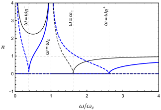
Figure 1: Index of refraction $n_{R}$, under the condition (31). The dashed blue (black) line corresponds to the imaginary piece of $n_{R}$ ($n_{-}$), while the solid blue (black) line represents the real piece of $n_{R}$ ($n_{-}$). Note that the chiral factor opens a new lossy window near the origin and enlarges the second absorption zone. Here, $\omega_{c}=\omega_{p}$, $\lvert\mathbf{V}\rvert=2\omega_{p}$, and $\omega_{c}=1$ $\mathrm{rad}$ $s^{-1}$.

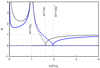
Figure 2: Index of refraction $n_{R}$, under the condition (33). The dashed blue (black) line corresponds to the imaginary piece of $n_{R}$ ($n_{-}$), while the solid blue (black) line represents the real piece of $n_{R}$ ($n_{-}$). The chiral factor increases the absorption zone near resonance. Here, $\omega_{c}=\omega_{p}$, $\lvert\mathbf{V}\rvert=0.5\omega_{p}$, and $\omega_{c}=1$ $\mathrm{rad}$ $s^{-1}$.

II.1.2 About the index $n_{L}$

The index $n_{L}$, given in Eq. (27), has no positive root under the condition (31) (no cutoff frequency) and one cutoff frequency under the condition (33). Its features are described below.

1. For $\omega\rightarrow 0$, under the condition (31), the presence of $\lvert\mathbf{V}\rvert$ renders the refractive index real and positively divergent at the origin, $n_{L}\rightarrow+\infty$, differing from the usual index $n_{+}$ (5), which is complex and divergent, $\mathrm{Im}[n_{+}]\rightarrow\infty$, at the origin. This behavior is similar to what is observed in the index $n_{L}$ of the chiral MCFJ model examined in Ref. [67].

2. For $\omega>0$, the index $n_{L}$ is always real, $\mathrm{Im}[n_{L}]=0$. Thus wave propagation occurs for any frequency. The real and imaginary parts of $n_{L}$ are represented in Fig. 3.

3. Under the condition (33), $n_{L}$ presents a cutoff frequency, $\omega_{L}$, given by Eq. (32). Therefore, an absorption zone appears for $0<\omega<\omega_{L}$, where $\mathrm{Im}\left[n_{L}\right]\neq 0$, as depicted in Fig. 4.

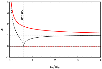
Figure 3: Refractive index $n_{L}$ (red lines) for condition (31) and index $n_{+}$ (black lines) of Eq. (5). The dashed (solid) lines correspond to the imaginary (real) pieces of $n_{L}$ and $n_{+}$. The chiral factor suppresses the absorption window. Here, $\omega_{c}=\omega_{p}$, $\lvert\mathbf{V}\rvert=2\omega_{p}$, and $\omega_{c}=1$ $\mathrm{rad}$ $s^{-1}$.

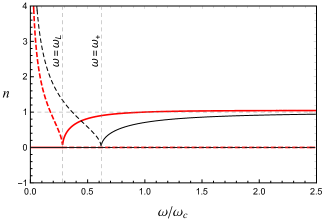
Figure 4: Refractive index $n_{L}$ (red lines) for condition (33). Refractive index $n_{+}$ (black lines) of Eq. (5). The dashed (solid) lines correspond to the imaginary (real) pieces of $n_{L}$ and $n_{+}$. The chiral factor narrows the absorption zone and enhances the attenuation-free propagation regime. Here, $\omega_{c}=\omega_{p}$, $\lvert\mathbf{V}\rvert=0.5\omega_{p}$, and $\omega_{c}=1$ $\mathrm{rad}$ $s^{-1}$.

We observe that the indices $n_{R}$ and $n_{L}$ are always positive, implying the inexistence of negative refraction, a phenomenon that was reported in the context of the MCFJ cold plasmas in the presence of the chiral timelike background factor.

The results of this Sec. II.1 may be compared with the case of wave propagation along the magnetic field with the MCFJ timelike background, examined in Sec. IV of Ref [67], whose scenario was richer by the attainment of four distinct indices and negative refraction, which typically occurs in bi-isotropic media as well [69, 70]. In the present case, however, there appear only two positive indices (no negative refraction). Nevertheless, regarding the propagation and absorption properties, the present chiral vector case is more involved since two absorption zones are opened under the condition (31), while in the analogous situation of Ref. [67] only one absorption zone was reported.

II.1.3 Dispersion relations behavior

The behavior of the dispersion relations can be visualized in plots $\omega\times k$. In this section, the dispersion relations associated with the circular modes, connected to the indices $n_{R}$ and $n_{L}$, are presented in dimensionless plots, $\left(\omega/\omega_{c}\right)\times\left(k/\omega_{c}\right)$. The dispersion relation associated with $\pm n_{R}$, under the condition (31), is depicted in Fig. 5. The propagation occurs for $\omega_{R}^{-}<\omega<\omega_{c}$ and $\omega>\omega_{R}^{+}$, while two absorption windows appear: $\omega_{c}<\omega<\omega_{R}^{+}$ and $0<\omega<\omega_{R}^{-}$. On the other hand, for the condition (33), the behavior is showed in Fig. 6, where the propagation occurs for $0<\omega<\omega_{c}$ and $\omega>\omega_{R}^{+}$, and the absorption happens for $\omega_{c}<\omega<\omega_{R}^{+}$. Both Figs. 5 and 6 illustrate enhanced absorption zones.

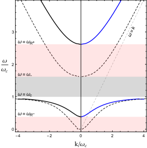
Figure 5: Dispersion relations related to refractive indices $n_{R}$ (solid blue line) and $-n_{R}$ (solid black line), under the condition (31). The dashed black line represents the indices of the standard case, $\pm n_{-}$. The highlighted area in red indicates the enlargement of the absorption zone for $n_{R}$ in relation to the gray absorption zone of the usual indices ($\pm n_{-}$). Here, we have used $\omega_{c}=\omega_{p}$ and $\lvert\mathbf{V}\rvert=2\omega_{p}$, with $\omega_{c}=1$ $\mathrm{rad}$ $s^{-1}$.

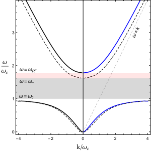
Figure 6: Plot of the dispersion relations related to refractive indices $n_{R}$ (solid blue line) and $-n_{R}$ (solid black line), under the condition (33). The dashed black line corresponds to the indices of the usual case ($\pm n_{-}$). The highlighted area in red indicates the absorption zone amplification for $n_{R}$ in comparison with the one of $\pm n_{-}$. Here, we have used $\omega_{c}=\omega_{p}$ and $\lvert\mathbf{V}\rvert=0.5\omega_{p}$, with $\omega_{c}=1$ $\mathrm{rad}$ $s^{-1}$.

Figure 7 illustrates the dispersion relations associated with $\pm n_{L}$ for condition (31), where the propagation occurs for $\omega>0$, being compatible with the absence of absorption zone, see Fig. 3. Considering the condition (33), the dispersion relation is depicted in Fig. 8, where there is an unusual absorption zone in $0<\omega<\omega_{L}$, while the propagation appears for $\omega>\omega_{L}$. In these two latter cases, the absorption zone is reduced in comparison to the zone of the usual indices, $\pm n_{+}$, $0<\omega<\omega_{+}$.

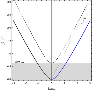
Figure 7: Dispersion relations associated with the refractive indices $n_{L}$ (solid blue line) and $-n_{L}$ (solid black line), under the condition (31). The dashed black line corresponds to the indices of the usual case ($\pm n_{+}$). The highlighted area in gray indicates the absorption zone for the indices $\pm n_{+}$, where one notices the absence of absorption for $n_{L}$. Here, we have used $\omega_{c}=\omega_{p}$ and $\lvert\mathbf{V}\rvert=2\omega_{p}$, with $\omega_{c}=1$ $\mathrm{rad}$ $s^{-1}$.

An interesting point is that the refractive indices $n_{R,L}$, represented by blue lines in Figs. 5, 6, 7, 8, do not become negative under influence of the chiral vector $\mathbf{V}$, allowing the plots $\omega\times k$ to remain centered at $k=0$. This is not the case for cold plasmas under the timelike CFJ electrodynamics [67], where the scalar chiral parameter $V_{0}$ induces zones of negative refraction (negative refractive indices), decentralizing the curves $\omega\times k$. See Ref. [67].

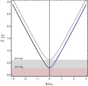
Figure 8: Dispersion relations associated with the refractive indices $n_{L}$ (solid blue line) and $-n_{L}$ (solid black line), under the condition (33). The dashed black line corresponds to the indices of the usual case ($\pm n_{+}$). The highlighted area in red indicates the absorption zone for $n_{L}$, narrowed in comparison to the absorption zone associated with $\pm n_{+}$. Here, we have used $\omega_{c}=\omega_{p}$ and $\lvert\mathbf{V}\rvert=0.5\omega_{p}$, with $\omega_{c}=1$ $\mathrm{rad}$ $s^{-1}$.

II.1.4 Low-frequency helicon modes

There are low-frequency plasma modes that propagate along the magnetic field axis, called helicons. In a usual magnetized plasma, there exists only RCP helicon modes, for which the refractive index (5) yields

$$n_{-} =\omega_{p}\sqrt{\frac{1}{\omega\omega_{c}}},$$ (34)

in the low-frequency regime,

$$\omega\ll\omega_{p},\quad\omega_{c}\ll\omega_{p},\quad\omega\ll\omega_{c}.$$ (35)

Considering the circular electromagnetic modes associated with the indices (26) and (27), the corresponding helicons indices are

$$\bar{n}_{R} =\sqrt{\frac{\omega_{p}^{2}}{\omega\omega_{c}}-\frac{\lvert\mathbf{V}\rvert}{\omega}},$$ (36a)

$$\bar{n}_{L} =\sqrt{\frac{\lvert\mathbf{V}\rvert}{\omega}-\frac{\omega_{p}^{2}}{\omega\omega_{c}}},$$ (36b)

where we have used the “bar” notation to indicate the helicons quantities. Due to the chiral vector, $\lvert\mathbf{V}\rvert$, one obtains expressions for both RCP and LCP helicons. As $\bar{n}_{R}^{2}=-\bar{n}_{L}^{2}$, one of these indices is imaginary when the other is real. In fact, $\bar{n}_{R}$ becomes imaginary for $\lvert\mathbf{V}\rvert>\omega_{p}^{2}/\omega_{c}$, while $\bar{n}_{L}$ is imaginary for $\lvert\mathbf{V}\rvert<\omega_{p}^{2}/\omega_{c}$. It means that RCP and LCP helicons do not propagate simultaneously. Indeed, only one of the modes in Eq. (36) can propagate for each value of $\lvert\mathbf{V}\rvert$ adopted. In this context, note that the usual cold plasma helicon mode is recovered in the limit $\lvert\mathbf{V}\rvert\rightarrow 0$, for which the helicon index $\bar{n}_{R}$ yields the usual result of Eq. (34), while $\bar{n}_{L}$ becomes purely imaginary, indicating the absence of propagation.

II.1.5 Rotatory power

Chiral media are featured by optical activity, usually described in terms of the rotation of the polarization (birefringence) that takes place when RCP and LCP modes propagate at different phase velocities. Such a rotation is measured in terms of the rotatory power, useful to performing optical characterization of multiple systems, as crystals [71, 72], organic compounds [74, 73], graphene phenomena at terahertz band [75], gas of fast-spinning molecules [76], chiral metamaterials [77, 78, 79], chiral semimetals [80, 81], in the determination of the rotation direction of pulsars [82]. The RP may be dispersive (depend on the frequency) [85, 84, 83]. The RP is defined as

$$\delta=-\frac{\omega}{2}\left(\mathrm{Re}[n_{L}]-\mathrm{Re}[n_{R}]\right),$$ (37)

where $n_{L}$ and $n_{R}$ are the refractive indices for different circular polarizations. For the case the background vector is parallel to the magnetic field, see Sec. II.1, the refractive indices, given by Eqs. (26) and (27), yield

$$\delta=-\frac{\omega}{2}\mathrm{Re}\left[\sqrt{R_{+}}-\sqrt{R_{-}}\right],$$ (38)

where $R_{\pm}$ is given by

$$R_{\pm}=1-\frac{\omega_{p}^{2}}{\omega\left(\omega\pm\omega_{c}\right)}\pm\frac{\lvert\mathbf{V}\lvert}{\omega}.$$ (39)

The behavior of the RP (38) is depited in Fig. 9, being negative for the interval $0<\omega<\hat{\omega}$ and positive for $\hat{\omega}<\omega<\omega_{c}$. For $\omega>\omega_{c}$, the RP is always negative, exhibiting a sharp behavior at $\omega=\omega_{R}$, the point at which the real piece of $n_{R}$ assumes non-zero values again (see Fig. 1). The frequency $\hat{\omega}$,

$$\hat{\omega}=\sqrt{\omega_{c}\left(\omega_{c}-\omega_{p}^{2}/\lvert\mathbf{V}\rvert\right)},$$ (40)

obtained from the expressions (38) and (39), indicates where the RP changes sign, as shown in Fig. 9. Note that $\hat{\omega}$ is real only for the condition (31). Hence the RP reversion only occurs in this case, as confirmed in Fig. 9. In fact, under the condition (33), the corresponding RP depicted in Fig. 10 is not endowed with sign reversal, in a close behavior to the standard RP.

It is worthy to remark that the RP reversion is observed in graphene systems [75], Weyl metals and semimetals with low electron density with chiral conductivity [80, 81], and bi-isotropic dielectrics with magnetic chiral conductivity [87]. Such a reversion does not occurs in conventional cold plasma, but it takes places in rotating plasmas [86] and in the MCJF plasma with chiral pseudoscalar factor [67]. Therefore, RP reversion may be considered a signature of chiral MCFJ nonrotating cold plasmas.

Furthermore, it is important to pay attention to the intervals $0<\omega<\omega_{R}^{-}$ and $\omega_{c}<\omega<\omega_{R}^{+}$, where the refractive index $n_{R}$ is imaginary and the RP receives contribution only from the index $n_{L}$, exhibiting an approximately linear increasing magnitude, the opposite of the $n_{L}$ profile. For $\omega>\omega_{R}^{+}$, the modes associated with the $n_{L}$ and $n_{R}$ propagate and contribute to the RP, whose magnitude diminishes monotonically with $\omega$, tending to the asymptotic value, $-|{\bf{V}}|/2$, as shown in Fig. 9. In fact, in the high-frequency limit, $\omega>>\omega_{p},\omega_{c}$, the refractive indices $n_{L}$ and $n_{R}$ provide (at first order)

$$n_{L,R}\simeq\,1\pm\frac{\lvert\mathbf{V}\rvert}{2\omega},$$ (41)

so that the rotatory power asymptotic value is

$$\delta\simeq-\frac{\lvert\mathbf{V}\rvert}{2},$$ (42)

a result that holds even in the absence of the magnetic field. This asymptotic limit differs from the behavior of a cold usual plasma, whose RP decays as $1/\omega^{2}$ for high frequencies, tending to zero for $\omega>>\omega_{p},\omega_{c}$. See the dashed line in Fig. 9.

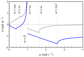
Figure 9: The solid blue line represents the rotatory power (38) defined by the refractive index $n_{L}$ and $n_{R}$, for the condition (31). The dashed black line corresponds to the usual rotatory power for a conventional cold plasma. The chiral factor determines the RP sign reversion at $\omega<\hat{\omega}$ and a constant asymptotic value, $-|\mathbf{V}|/2$, for high frequencies. Here, we have used $\omega_{c}=\omega_{p}$, $\lvert\mathbf{V}\rvert=2\omega_{p}$, and $\omega_{c}=1$ $\mathrm{rad}$ $s^{-1}$.

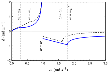
Figure 10: Solid blue lines: rotatory power (38) associated with the refractive indices $n_{L}$ and $n_{R}$ for the condition (33). The dashed line represents the usual rotatory power for a usual cold plasma. Small deviations of RP are originated from the chiral factor. The main difference in comparison with the usual case is the non-null asymptotical value, $-|\mathbf{V}|/2$, for high frequencies. Here, we have used $\omega_{c}=\omega_{p}$, $\lvert\mathbf{V}\rvert=0.5\omega_{p}$, and $\omega_{c}=1$ $\mathrm{rad}$ $s^{-1}$.

II.1.6 Dichroism coefficients

In the zones where the indices are complex, there occurs absorption. When circularly polarized modes undergo absorption at different degrees, dichroism takes place, working as another parameter for optical characterization. It could be used to distinguish between Dirac and Weyl semimetals [88], perform enantiomeric discrimination [89, 90], and for developing graphene-based devices at terahertz frequencies [91]. Dichroism for LCP and RCP waves is expressed in terms of the coefficient,

$$\delta_{d}=-\frac{\omega}{2}\left(\mathrm{Im}[n_{L}]-\mathrm{Im}[n_{R}]\right).$$ (43)

For the condition (31), $n_{R}$ has non-null imaginary parts in the intervals $0<\omega<\omega_{R}^{-}$ and $\omega_{c}<\omega<\omega_{R}^{+}$, while $n_{L}$ is always real (for $\omega>0$). In this case, the dichroism coefficient is written as

$$\delta_{d}=\begin{cases}\text{$\frac{\omega}{2}\sqrt{R_{-}},$}&\quad\text{for $0<\omega<\omega_{R}^{-},$}\\ \text{$0,$}&\quad\text{for $\omega_{R}^{-}<\omega<\omega_{c},$}\\ \text{$\frac{\omega}{2}\sqrt{R_{-}},$}&\quad\text{for $\omega_{c}<\omega<\omega_{R}^{+},$}\\ \text{$0,$}&\quad\text{for $\omega>\omega_{R}^{+},$}\end{cases}$$ (44)

with $R_{-}$ of Eq. (39). Such a coefficient is depicted in Fig. 11.

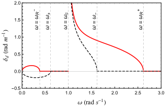
Figure 11: Dichroism coefficient of Eq. (44)) (red solid lines) associated with $n_{L}$ and $n_{R}$, under the condition (31). The black dashed line represents the dichroism coefficient of a usual cold plasma. Here, $\omega_{c}=\omega_{p}$, $\lvert\mathbf{V}\rvert=2\omega_{p}$, and $\omega_{c}=1$ $\mathrm{rad}$ $s^{-1}$.

Considering the condition (33), both $n_{R}$ and $n_{L}$ have non-null imaginary parts in the intervals $\omega_{c}<\omega<\omega_{R}^{+}$ and $0<\omega<\omega_{L}$, respectively, in which the dichroism coefficient is non-null,

$$\delta_{d}=\begin{cases}\text{$-\frac{\omega}{2}\sqrt{R_{+}}$},&\quad\text{for $0<\omega<\omega_{L}$},\\ \text{$+\frac{\omega}{2}\sqrt{R_{-}}$},&\quad\text{for $\omega_{c}<\omega<\omega_{R}^{+}$}.\\ \end{cases}$$ (45)

The general behavior of (45) is exhibited in Fig. 12.

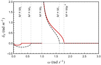
Figure 12: Dichroism coefficient of Eq. (45) (solid red lines) associated with $n_{L}$ and $n_{R}$, under the condition (33). The dashed line represents the dichroism coefficient for a conventional cold plasma. Here, we have set $\omega_{c}=\omega_{p}$, $\lvert\mathbf{V}\rvert=0.5\omega_{p}$, and $\omega_{c}=1$ $\mathrm{rad}$ $s^{-1}$.

II.2 Chiral vector orthogonal to the magnetic field

In the scenario where the background vector is orthogonal to the magnetic field, $\beta\to\pi/2$, and the dispersion relation (22) reads

$$P\left[D^{2}-\left(n^{2}-S\right)^{2}\right]+\left(\lvert\mathbf{V}\rvert^{2}/\omega^{2}\right)\left(S-n^{2}\right)=0,$$ (46)

yielding two refractive indices:

$$\left(n_{A}\right)^{2}=S-\frac{\lvert\mathbf{V}\rvert^{2}}{2P\omega^{2}}+\frac{1}{P}\sqrt{P^{2}D^{2}+\frac{\lvert\mathbf{V}\rvert^{4}}{4\omega^{4}}},$$ (47)

$$\left(n_{B}\right)^{2}=S-\frac{\lvert\mathbf{V}\rvert^{2}}{2P\omega^{2}}-\frac{1}{P}\sqrt{P^{2}D^{2}+\frac{\lvert\mathbf{V}\rvert^{4}}{4\omega^{4}}}.$$ (48)

From Eq. (20), mixed elliptical polarizations are evaluated for the propagating modes,

$$n_{A,B}\quad\rightarrow\quad\mathbf{E}_{A,B}=C\begin{bmatrix}-\zeta\\ 1\\ -i\lvert\mathbf{V}\rvert\left(n_{A,B}^{2}-S\right)/(\omega\bar{\kappa}P)\end{bmatrix},$$ (49a)

where

$$C=\frac{\lvert\bar{\kappa}\rvert}{\sqrt{\left(n^{2}-S\right)^{2}\left[\left(\lvert\mathbf{V}\rvert/\omega P\right)^{2}+\sin^{2}\phi\right]+D^{2}\cos^{2}\phi+\lvert\bar{\kappa}\rvert^{2}}},$$ (49b)

$$\zeta=\frac{\left(\left(n^{2}-S\right)^{2}-D^{2}\right)\cos\phi\sin\phi+iD\left(n^{2}-S\right)}{\left|\bar{\kappa}\right|^{2}},$$ (49c)

$$\bar{\kappa}=\left(n^{2}-S\right)\cos\phi-iD\sin\phi.$$ (49d)

In Eq. (49a), one notices a longitudinal imaginary component. The transversal sector is, in general, elliptically polarized since $\zeta$ is a complex quantity. Starting from Eq. (49a) and setting $\lvert\mathbf{V}\rvert\rightarrow 0$, the usual RCP and LCP modes are recovered, which is an expected correspondence.

The refractive indices given in (47) and (48) have real positive roots given by

$$\omega_{A1,B} =\frac{1}{6}\sqrt{8\omega_{c}^{2}\mp 2\sqrt[3]{\frac{\mp 2}{U}}f_{1}+(\mp 2)^{2/3}\sqrt[3]{U}+2\left|\mathbf{V}\right|^{2}},$$ (50)

$$\omega_{A2} =\frac{1}{6}\sqrt{8\omega_{c}^{2}+\frac{(2)^{4/3}(-1)^{2/3}f_{1}}{\sqrt[3]{U}}-f_{4}},$$ (51)

where

$$U =11\omega_{c}^{6}+f_{2}+3\sqrt{3}\sqrt{-c^{4}\left(5\omega_{c}^{8}+f_{3}\right)},$$ (52a)

$$f_{1} =4\omega_{c}^{4}+2\omega_{c}^{2}\left|\mathbf{V}\right|^{2}+\left|\mathbf{V}\right|^{4},$$ (52b)

$$f_{2} =-12\omega_{c}^{4}\left|\mathbf{V}\right|^{2}+6\omega_{c}^{2}\left|\mathbf{V}\right|^{4}+2\left|\mathbf{V}\right|^{6},$$ (52c)

$$f_{3} =24\omega_{c}^{6}\left|\mathbf{V}\right|^{2}+4\omega_{c}^{4}\left|\mathbf{V}\right|^{4}+12\omega_{c}^{2}\left|\mathbf{V}\right|^{6}+4\left|\mathbf{V}\right|^{8},$$ (52d)

$$f_{4} =\sqrt[3]{-1}\left(2\right)^{2/3}\sqrt[3]{U}+2\left|\mathbf{V}\right|^{2},$$ (52e)

being $\omega_{A1,2}$ associated to $n_{A}$ and $\omega_{B}$ associated to $n_{B}$.

II.2.1 About the index $n_{A}$

The refractive index $n_{A}$, given in Eq. (47), has two positive roots, $\omega_{A1}$ and $\omega_{A2}$, as illustrated in Fig. 13, where we observe:

1. For $\omega\rightarrow 0$, the index is imaginary and tends to infinity, $n_{A}\rightarrow+i\infty$, the same behavior of the usual magnetized plasma index $n_{+}$ near the origin.

2. For $0<\omega<\omega_{A1}$, it holds $\mathrm{Re}\left[n_{A}\right]=0$, $\mathrm{Im}\left[n_{A}\right]\neq 0$, defining an absorption zone.

3. For $\omega_{A1}<\omega<\omega_{c}$, $n_{A}$ is real, $\mathrm{Re}\left[n_{A}\right]>0$ and $\mathrm{Im}\left[n_{A}\right]=0$, opening an intermediary propagation zone that does not appear in the usual case. Compare the black and red lines in Fig. 13.

4. For $\omega\rightarrow\omega_{c}$, there occurs a resonance, $n_{A}\rightarrow\infty$, at the cyclotron frequency, behavior not reported in the standard case. For $\omega_{c}<\omega<\omega_{A2}$, $n_{A}$ is imaginary, that is, $\mathrm{Im}\left[n_{A}\right]\neq 0$, $\mathrm{Re}\left[n_{A}\right]=0$, thus another absorption zone is allowed.

5. For $\omega>\omega_{A2}$, there is a propagating zone, in which the index $n_{A}$ is always positive and real, with $n_{A}\rightarrow 1$ in the high-frequency limit. See Fig. 13.

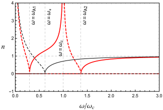
Figure 13: Refractive index $n_{A}$ (red lines) and $n_{+}$ (black lines) of Eq. (5). The dashed (solid) lines correspond to the imaginary (real) pieces of $n_{A}$ and $n_{+}$. There is an intermediary propagation zone in the range $\omega_{A1}<\omega<\omega_{c}$ and a new absorption interval defined for $\omega_{c}<\omega<\omega_{A2}$. Here, $\omega_{c}=\omega_{p}$, $\lvert\mathbf{V}\rvert=2\omega_{p}$, and $\omega_{c}=1$ $\mathrm{rad}$ $s^{-1}$.

II.2.2 About the index $n_{B}$

The index $n_{B}$ in Eq. (48) has only one cutoff frequency, represented by $\omega_{B}$. Its real and imaginary parts are illustrated in Fig. 14.

1. In the limit $\omega\rightarrow 0$, the index $n_{B}$ is real and tends to infinity, $n_{B}\rightarrow+\infty$. For $0<\omega<\omega_{c}$, the index $n_{B}$ is real, with $\mathrm{Im}[n_{B}]=0$, a behavior close to one of standard magnetized plasmas.

2. For $\omega\rightarrow\omega_{c}$, $n_{B}\rightarrow\infty$, and there is a resonance at the cyclotron frequency. This behavior also occurs in the usual case. For $\omega_{c}<\omega<\omega_{B}$, the index is imaginary, $\mathrm{Re}[n_{B}]=0$, $\mathrm{Im}[n_{B}]\neq 0$, describing an absorption zone, that is larger than the usual one, since $\omega_{B}>\omega_{-}$. See Fig. 14.

3. For $\omega>\omega_{B}$, one has a propagating zone, where $n_{B}$ is always real and positive, with $n_{B}\rightarrow 1$ in the high-frequency limit.

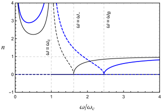
Figure 14: Refractive index $n_{B}$ (blue lines) and $n_{-}$ (black lines) of Eq. (5). The dashed (solid) lines correspond to the imaginary (real) pieces of $n_{B}$ and $n_{-}$. The intermediary absorption zone, $\omega_{c}<\omega<\omega_{B}$, has now amplified length. Here, $\omega_{c}=\omega_{p}$, $\lvert\mathbf{V}\rvert=2\omega_{p}$, and $\omega_{c}=1$ $\mathrm{rad}$ $s^{-1}$.

The results of the present section can not be compared with the ones of Ref. [67], since the defining condition of this section – a chiral vector orthogonal to the magnetic field – is not accomplishable in the scenario of a scalar chiral factor [67].

II.2.3 Optical effects

Considering the configuration of the background vector orthogonal to the magnetic field, the refractive indices (47) and (48) are not associated with circularly polarized modes [see Eq. (49a)]. In this panorama, the birefringence is better characterized in terms of the phase shift per unit length, given by

$$\frac{\Delta}{d}=\frac{2\pi}{\lambda_{0}}\left(\mathrm{Re}[n_{A}]-\mathrm{Re}[n_{B}]\right),$$ (53)

or explicitly

$$\frac{\Delta}{d}=\frac{2\pi}{\lambda_{0}}\left(\sqrt{S-\frac{\lvert\mathbf{V}\rvert^{2}}{2P\omega^{2}}+\Xi_{AB}}-\sqrt{S-\frac{\lvert\mathbf{V}\rvert^{2}}{2P\omega^{2}}-\Xi_{AB}}\right),$$ (54)

where

$$\Xi_{AB}\left(\omega,\lvert\mathbf{V}\rvert\right)=\sqrt{D^{2}+\frac{\lvert\mathbf{V}\rvert^{4}}{4P^{2}\omega^{4}}}.$$ (55)

In the high-frequency limit $\omega>>\left(\omega_{c},\omega_{p}\right)$, the phase shift is

$$\frac{\Delta}{d}\simeq\,-\frac{2\pi}{\lambda_{0}}\sqrt{\frac{2\omega_{c}\omega_{p}^{2}}{\left(2\omega^{2}-\lvert\mathbf{V}\rvert^{2}\right)\omega}}.$$ (56)

As for absorption effect for non-circularly propagating modes, one can define the difference of absorption between the two modes per unit length, written as

$$\frac{\Delta_{Im}}{d}=\frac{2\pi}{\lambda_{0}}\left(\mathrm{Im}[n_{A}]-\mathrm{Im}[n_{B}]\right).$$ (57)

For $\omega_{c}<\omega<\omega_{A2}$, the indices $n_{A}$ and $n_{B}$ are purely imaginary, see the corresponding dashed lines in Fig. 13 and 14. In this range, the absorption factor (57) is

$$\frac{\Delta_{Im}}{d}=\frac{2\pi}{\lambda_{0}}\left[\sqrt{\frac{\lvert\mathbf{V}\rvert^{2}}{2P\omega^{2}}-\Xi_{AB}-S}-\sqrt{\frac{\lvert\mathbf{V}\rvert^{2}}{2P\omega^{2}}+\Xi_{AB}-S}\right].$$ (58)

For $\omega<\omega_{A1}$, only the mode associated whit $n_{A}$ is absorbed. In this case, we can write the absorption coefficient, $\gamma=2\omega\mathrm{Im}[n]$, explicitly given by

$$\gamma=2\omega\sqrt{\frac{\lvert\mathbf{V}\rvert^{2}}{2P\omega^{2}}-\Xi_{AB}-S}.$$ (59)

III WAVE PROPAGATION ORTHOGONAL TO THE MAGNETIC FIELD

For propagation orthogonal to the magnetic field, we can implement $\mathbf{n}=\left(n_{x},n_{y},0\right)$ in Eq. (19). Furthermore, we propose a parameterization for the wave propagation in the plane orthogonal to the magnetic field in terms of the angle $\alpha$ between the propagation direction and the $x$-axis,

$$\mathbf{n}=n\left(\cos\alpha,\sin\alpha,0\right).$$ (60)

Thus, Eq. (18) now reads

$$\begin{bmatrix}n^{2}-n^{2}\cos^{2}\alpha-S&-n^{2}\cos\alpha\sin\alpha+iD+i\left(\lvert\mathbf{V}\rvert/\omega\right)\cos\beta&-i\left(\lvert\mathbf{V}\rvert/\omega\right)\sin\phi\sin\beta\\ -n^{2}\cos\alpha\sin\alpha-iD-i\left(\lvert\mathbf{V}\rvert/\omega\right)\cos\beta&{n^{2}-n^{2}\sin^{2}\alpha-S}&+i\left(\lvert\mathbf{V}\rvert/\omega\right)\cos\phi\sin\beta\\ +i\left(\lvert\mathbf{V}\rvert/\omega\right)\sin\phi\sin\beta&-i\left(\lvert\mathbf{V}\rvert/\omega\right)\cos\phi\sin\beta&n^{2}-P\end{bmatrix}\begin{bmatrix}\delta E_{x}\\ \delta E_{y}\\ \delta E_{z}\end{bmatrix}=0.$$ (61)

The null determinant condition provides the following dispersion relation:

$$\left(n^{2}-P\right)\left[D^{2}+S\left(n^{2}-S\right)\right)]-\left(\lvert\mathbf{V}\rvert/2\omega\right)^{2}\Theta=0,$$ (62)

where

$$\Theta =\left[2(P+S)-3n^{2}\right]+8D\omega\left(P-n^{2}\right)\cos\beta/\lvert\mathbf{V}\rvert$$

$$-\left(n^{2}-2P+2S\right)\cos(2\beta)+2n^{2}\sin^{2}(\beta)\cos(2(\alpha-\phi)).$$ (63)

III.1 Chiral vector parallel to the magnetic field

A chiral vector parallel to the magnetic field, $\mathbf{V}\parallel\mathbf{B_{0}}$, implies $\beta=0$, whose replacement in Eq. (62), yields the index $n_{T}^{2}$,

$$n_{T}^{2}=1-\frac{\omega_{p}^{2}}{\omega^{2}},$$ (64)

also given in Eq. (7), being associated with the same usual linear transversal mode.

It also provides a modified refractive index,

$$n_{\chi}^{2}=\frac{S^{2}-D^{2}}{S}-\frac{\lvert\mathbf{V}\rvert^{2}+2D\lvert\mathbf{V}\rvert\omega}{S\omega^{2}},$$ (65)

associated with the elliptical propagating mode,

$$n_{\chi}\quad\rightarrow\quad\mathbf{E}=C_{\chi}\begin{bmatrix}-\zeta_{\chi}\\ 1\\ 0\end{bmatrix},$$ (66)

where

$$C_{\chi} =\frac{1}{\sqrt{\lvert\zeta_{\chi}\rvert^{2}+1}},$$ (67a)

$$\zeta_{\chi} =\frac{i\left[D+\left(\left|\mathbf{V}\right|/\omega\right)\right]-n^{2}\cos\alpha\sin\alpha}{n^{2}\sin^{2}\alpha-S}.$$ (67b)

The refractive index $n_{\chi}$ has three cutoff frequencies, $\omega_{R}^{\pm}$ and $\omega_{L}$, given in Eq. (30) and Eq. (32).

III.1.1 About the index $n_{\chi}$

The refractive index $n_{\chi}$ has the refractive index $n_{O}$ as the conventional cold plasma counterpart, given in (8), sharing with it the same resonance frequency

$$\omega_{cp}=\sqrt{\omega_{c}^{2}+\omega_{p}^{2}}.$$ (68)

Under the condition (33), $n_{\chi}$ shows two cutoff frequencies, $\omega_{R}^{+}$ and $\omega_{L}$, the same ones of Eqs. (30) and (32), respectively. These frequencies are marked in Fig. 15. Moreover, we point out:

1. For $0<\omega<\omega_{L}$, $n_{\chi}$ is imaginary, corresponding to an absorption zone smaller than the usual one, $0<\omega<\omega_{+}$, since $\omega_{L}<\omega_{+}$. See the black dashed line in Fig. 15.

2. For $\omega_{L}<\omega<\omega_{cp}$, there occurs $\mathrm{Re}[n_{\chi}]\neq 0$ and $\mathrm{Im}[n_{\chi}]=0$, defining a propagation zone larger than the standard case one ($\omega_{+}<\omega<\omega_{cp}$).

3. For $\omega\rightarrow\omega_{cp}$, there occurs a resonance, $n_{\chi}\rightarrow+\infty$, the same behavior of the usual case. For $\omega_{cp}<\omega<\omega_{R}^{+}$, $\mathrm{Re}[n_{\chi}]=0$ and $\mathrm{Im}[n_{\chi}]\neq 0$, and another absorption zone is allowed.

4. For $\omega>\omega_{R}^{+}$, the quantity $n_{\chi}$ is always positive, corresponding to a propagation zone, which in the usual case begins at $\omega=\omega_{-}$.

Under the condition (31), $n_{\chi}$ has two roots, $\omega_{R}^{\pm}$, and similar characteristics to those described above, as shown in Fig. 16.

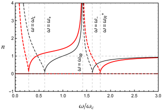
Figure 15: Red line: index $n_{\chi}$ under the condition (33). Black line: index $n_{O}$. Dashed (solid) lines represent the imaginary (real) pieces of $n_{\chi}$ and $n_{O}$. Note that the chiral vector factor shortens the first absorption zone and slightly augments the second one. Here, we have used: $\omega_{c}=\omega_{p}$, $\lvert\mathbf{V}\rvert=0.5\omega_{p}$, and $\omega_{c}=1$ $\mathrm{rad}$ $s^{-1}$.

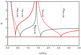
Figure 16: Red line: plot of the index $n_{\chi}$ under the condition (31). Black line: plot of the index $n_{O}$. Dashed (solid) lines represent the imaginary (real) pieces of $n_{\chi}$ and $n_{O}$. The chiral vector reduces the first absorption frequency window and enhances the second one. Here, we have used: $\omega_{c}=\omega_{p}$, $\lvert\mathbf{V}\rvert=2\omega_{p}$, and $\omega_{c}=1$ $\mathrm{rad}$ $s^{-1}$.

III.1.2 Optical effects

For the configuration of a background vector parallel to the magnetic field, the propagating modes obtained were described by elliptical and linear polarized vectors, associated with the refractive indices $n_{T}$ and $n_{\chi}$, respectively. In this case, the birefringence is evaluated employing the phase shift per unit length,

$$\frac{\Delta}{d}=\frac{2\pi}{\lambda_{0}}\left(\mathrm{Re}[n_{T}]-\mathrm{Re}[n_{\chi}]\right),$$ (69)

which for the indices (64) and (65), read

$$\frac{\Delta}{d}=\frac{2\pi}{\lambda_{0}}\left(\sqrt{P}-\sqrt{\frac{S^{2}-D^{2}}{S}-\frac{\lvert\mathbf{V}\rvert^{2}+2D\lvert\mathbf{V}\rvert\omega}{S\omega^{2}}}\right).$$ (70)

In the limit $\omega>>(\omega_{p},\omega_{c})$, using the parameters $S$, $D$, $P$ given in (4), such a phase shift reduces to:

$$\frac{\Delta}{d}=\frac{2\pi}{\lambda_{0}}\left(1-\sqrt{\frac{\omega^{2}-\lvert\mathbf{V}\rvert^{2}}{\omega^{2}}}\right).$$ (71)

In the usual case, where $\Delta/d\propto(n_{T}-n_{O})$, the phase shift is null in the high-frequency limit, a result recovered for $\lvert\mathbf{V}\rvert\rightarrow 0$ in (71). Thus, the chiral vector is responsible for an unusual dispersive birefringence in the high-frequency domain.

Concerning the absorption for non-circularly propagating modes, the difference of absorption between the two modes per unit length,

$$\frac{\Delta_{Im}}{d}=\frac{2\pi}{\lambda_{0}}\left(\mathrm{Im}[n_{T}]-\mathrm{Im}[n_{\chi}]\right),$$ (72)

which yields

$$\frac{\Delta_{Im}}{d}=\frac{2\pi}{\lambda_{0}}\left(\sqrt{P}-\sqrt{\frac{\lvert\mathbf{V}\rvert^{2}+2D\lvert\mathbf{V}\rvert\omega}{S\omega^{2}}-\frac{S^{2}-D^{2}}{S}}\right),$$ (73)

for the indices in Eqs. (64) and (65). It is non-null for $0<\omega<\omega_{L,R^{-}}$ and $\omega_{cp}<\omega<\omega_{R^{+}}$, under the condition (31) or (33), as showed in Figs. 15 and 16, respectively.

III.2 Background vector orthogonal to the magnetic field

Considering the chiral vector orthogonal to the magnetic field, $\mathbf{V}\perp\mathbf{B}_{0}$, we take $\beta\rightarrow\pi/2$ in Eq. (62), yielding two refractive indices

$$(n^{2}_{\Upsilon})_{\pm}=\frac{S(P+S)-D^{2}}{2S}-\frac{\lvert\mathbf{V}\rvert^{2}\sin^{2}(\alpha-\phi)}{2S\omega^{2}}\pm\frac{\eta}{4S\omega^{2}},$$ (74)

where

$$\eta =\sqrt{\Lambda^{2}-16S\omega^{2}\left(P\omega^{2}\left(S^{2}-D^{2}\right)-S\lvert\mathbf{V}\rvert^{2}\right)},$$ (75a)

$$\Lambda =2\left(D^{2}-S^{2}-PS\right)\omega^{2}-\lvert\mathbf{V}\rvert^{2}\cos\left(2\left(\alpha-\phi\right)\right)+\lvert\mathbf{V}\rvert^{2}.$$ (75b)

The indices $(n^{2}_{\Upsilon})_{\pm}$ are related to the following electromagnetic modes

$$(n_{\Upsilon})_{\pm}\quad\rightarrow\quad\mathbf{E_{\pm}}=C_{\Upsilon}\begin{bmatrix}-\zeta_{\Upsilon}\\ 1\\ \frac{\lvert\mathbf{V}\rvert\left(\cos\phi+i\zeta_{\Upsilon}\sin\phi\right)}{\omega\left(n_{\pm}^{2}-P\right)}\end{bmatrix},$$ (76)

where $C_{\Upsilon}$ is a normalization constant and

$$\zeta_{\Upsilon} =\frac{\zeta_{*}+iD\left(n^{2}\sin^{2}\alpha-S\right)\left(\cos^{2}\phi-\sin^{2}\phi\right)}{\left|\bar{\lambda}\right|^{2}},$$ (77a)

with

$$\zeta_{*} =\gamma+D^{2}\cos^{2}\phi-n^{2}\cos\alpha\sin\alpha\left(n^{2}\sin^{2}\alpha-S\right),$$ (77b)

$$\gamma =\left[\left(n^{2}\sin^{2}\alpha-S\right)^{2}+\left(n^{2}\cos\alpha\sin\alpha\right)^{2}\right]\sin\phi\cos\phi,$$ (77c)

$$\bar{\lambda} =\left(n^{2}\sin^{2}\alpha-S\right)\cos\phi-\left(n^{2}\cos\alpha\sin\alpha+iD\right)\sin\phi.$$ (77d)

The refractive indices in (74) have real and positive roots, $\omega_{\perp 1,2}$, associated with $\left(n_{\Upsilon}\right)_{+}$, and $\omega_{\perp+}$ associated with $\left(n_{\Upsilon}\right)_{-}$. These frequencies are not presented here, as they are very extensive and intricate solutions of a sixth-order equation in frequency.

In the following, some aspects of the indices $(n_{\Upsilon})_{\pm}$ will be discussed. Figures 17 and 18 illustrate the general behavior of $(n_{\Upsilon})_{\pm}$ for $\alpha-\phi=0$ ($\mathbf{V}\parallel\mathbf{n}$) and $\alpha-\phi=\pi/2$ ($\mathbf{V}\perp\mathbf{n}$), highlighted in red and blue lines, respectively.

III.2.1 About the index $(n_{\Upsilon})_{+}$

The refractive index $(n_{\Upsilon})_{+}$ can be compared to the index $n_{T}$, given in Eq. (64), which describes the usual transversal mode. We find that $(n_{\Upsilon})_{+}$ has two cutoff frequencies, $\omega_{\perp}$ and $\omega_{\perp 2}$. The behavior of $(n_{\Upsilon})_{+}$ is illustrated in Fig. 17, presenting the following features:

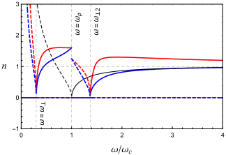
Figure 17: Red (blue) line indicates the index $(n_{\Upsilon})_{+}$ for $\alpha-\phi=0$ ($\alpha-\phi=\pi/2$). The black line illustrates $n_{T}$. Dashed (solid) lines represent the imaginary (real) pieces of $(n_{\Upsilon})_{+}$ and $n_{T}$. The chiral factor allows a new intermediary propagating zone for $\omega_{\perp}<\omega<\omega_{p}$, which is followed by a new absorption zone for $\omega_{p}<\omega<\omega_{\perp 2}$. Here, we have used: $\omega_{c}=\omega_{p}$, $\lvert\mathbf{V}\rvert=2\omega_{p}$, and $\omega_{c}=1$ $\mathrm{rad}$ $s^{-1}$.

1. For $0<\omega<\omega_{\perp}$, $(n_{\Upsilon})_{+}$ is imaginary, corresponding to an absorption zone.

2. For $\omega_{\perp}<\omega<\omega_{p}$, there occurs an attenuation-free propagation zone, where $\mathrm{Re}[(n_{\Upsilon})_{+}]\neq 0$ and $\mathrm{Im}[(n_{\Upsilon})_{+}]=0$. In the standard case, there is an absorption zone in this range.

3. For $\omega\rightarrow\omega_{p}$, $(n_{\Upsilon})_{+}$ has an unusual discontinuity, as shown in Fig. 17. For $\omega_{p}<\omega<\omega_{\perp 2}$, the index $(n_{\Upsilon})_{+}$ is imaginary and there appears an absorption zone. This aspect contrasts with the usual case, where $n_{T}$ is always real for $\omega>\omega_{p}$.

4. For $\omega>\omega_{\perp 2}$, $(n_{\Upsilon})_{+}$ is real, yielding an attenuation-free propagation zone.

III.2.2 About the index $(n_{\Upsilon})_{-}$

The index $(n_{\Upsilon})_{-}$ is a modification of the index $n_{O}$, given in Eq. (8), associated with the usual extraordinary mode. The former has a cutoff frequency at $\omega_{\perp+}$, as shown in Fig. 18. Some aspects of $(n_{\Upsilon})_{-}$ are summarized below.

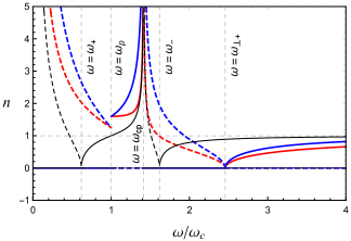
Figure 18: Red (blue) line: plot of the index $(n_{\Upsilon})_{-}$ for $\alpha-\phi=0$ ($\alpha-\phi=\pi/2$). Black line: plot of the index $n_{O}$. Dashed (solid) lines represent the imaginary (real) pieces of $(n_{\Upsilon})_{-}$ and $n_{O}$. The chiral factor enhances the length of the two absorption zones. Here, we have used: $\omega_{c}=\omega_{p}$, $\lvert\mathbf{V}\rvert=2\omega_{p}$, and $\omega_{c}=1$ $\mathrm{rad}$ $s^{-1}$.

1. For $0<\omega<\omega_{p}$, there occurs an absorption zone, where $\mathrm{Re}[(n_{\Upsilon})_{-}]=0$ and $\mathrm{Im}[(n_{\Upsilon})_{-}]\neq 0$. For $\omega\rightarrow\omega_{p}$, $(n_{\Upsilon})_{-}$ has a discontinuity, as noticed in Fig. 18. For $\omega_{p}<\omega<\omega_{cp}$, the index $(n_{\Upsilon})_{-}$ is real, corresponding to a propagation window. As $\omega_{p}>\omega_{+}$, the first absorption zone is enlarged while the first propagating window is shortened.

2. For $\omega\rightarrow\omega_{cp}$, $(n_{\Upsilon})_{-}\rightarrow\infty$, the same behavior of the usual case, as indicated in Fig. 18. For $\omega_{cp}<\omega<\omega_{\perp+}$, the index $(n_{\Upsilon})_{-}$ is purely imaginary and the associated mode is absorbed. As $\omega_{\perp+}>\omega_{-}$, this second absorption zone is also enlarged in comparison with the usual case one.

3. For $\omega>\omega_{\perp+}$, the quantity $(n_{\Upsilon})_{-}$ is always real, corresponding to an attenuation-free propagation zone. In the standard case, the propagation zone occurs for $\omega>\omega_{-}$.

III.2.3 Optical effects

For this configuration, there are two elliptical propagating modes associated with the refractive indices $(n_{\Upsilon})_{\pm}$, given in Eq. (74). Thus, the birefringence is measured in terms of the phase shift per unit length,

$$\frac{\Delta}{d}=\frac{2\pi}{\lambda_{0}}\left((n_{\Upsilon})_{+}-(n_{\Upsilon})_{-}\right).$$ (78)

Using the indices (74), the latter becomes

$$\frac{\Delta}{d}=\frac{2\pi}{\lambda_{0}}\left(\sqrt{\Pi-\Xi_{\perp-}}-\sqrt{\Pi-\Xi_{\perp+}}\right),$$ (79)

where

$$\Pi =\frac{S(P+S)-D^{2}}{2S},$$ (80a)

$$\Xi_{\perp\pm}\left(\omega,\lvert\mathbf{V}\rvert\right) =\frac{\lvert\mathbf{V}\rvert^{2}\sin^{2}(\alpha-\phi)}{2S\omega^{2}}\pm\eta/4.$$ (80b)

In the high-frequency limit, where $\omega>>\left(\omega_{c},\omega_{p}\right)$, Eq. (79) becomes

$$\frac{\Delta}{d}=\frac{\pi}{\lambda_{0}}\left(\sqrt{4+\lvert\mathbf{V}\rvert\xi_{+}/\omega^{2}}-\sqrt{4+\lvert\mathbf{V}\rvert\xi_{-}/\omega^{2}}\right),$$ (81a)

with

$$\xi_{\pm} =\pm\sqrt{\lvert\mathbf{V}\rvert^{2}+8\omega^{2}+\tilde{\gamma}\cos(2(\alpha-\phi))}$$

$$\phantom{=}-2\lvert\mathbf{V}\rvert^{2}\sin^{2}(\alpha-\phi),$$ (81b)

$$\tilde{\gamma} =\left(8\omega^{2}-2\lvert\mathbf{V}\rvert^{2}\right)+\lvert\mathbf{V}\rvert^{2}\cos(2(\alpha-\phi)).$$ (81c)

In this limit, the usual case result, $\Delta/d=0$, is recovered for $\lvert\mathbf{V}\rvert\rightarrow 0$.

Considering the lossy effect, one observes that electromagnetic modes associated with the refractive indices $(n_{\Upsilon})_{\pm}$ are absorbed for $\omega<\omega_{\perp}$ [see the dashed line in Figs. 17 and 18]. In this range, we can write the difference of absorption between the two modes per unit length,

$$\frac{\Delta_{Im}}{d}=\frac{2\pi}{\lambda_{0}}\left(\mathrm{Im}[(n_{\Upsilon})_{+}]-\mathrm{Im}[(n_{\Upsilon})_{-}]\right).$$ (82)

or

$$\frac{\Delta_{Im}}{d}=\frac{2\pi}{\lambda_{0}}\left(\sqrt{\Xi_{\perp-}-\Pi}-\sqrt{\Xi_{\perp+}-\Pi}\right).$$ (83)

For $\omega_{cp}<\omega<\omega_{\perp+}$, only $(n_{\Upsilon})_{-}$ has non-null imaginary piece. Then the corresponding absorption coefficient $\gamma=2\omega\mathrm{Im}[(n_{\Upsilon})_{-}]$ in this range is,

$$\gamma=2\omega\sqrt{\Xi_{\perp+}-\Pi}.$$ (84)

On the other hand, for $\omega_{p}<\omega<\omega_{\perp 2}$, only $(n_{\Upsilon})_{+}$ has an imaginary piece, which implies the following absorption coefficient:

$$\gamma=2\omega\sqrt{\Xi_{\perp-}-\Pi}.$$ (85)

In the usual case, the two electromagnetic modes are absorbed for $\omega<\omega_{+}$, since the indices $n_{T}$ and $n_{O}$ are purely imaginary in this range.

IV Final remarks

Electromagnetic wave propagation and absorption in a cold magnetized plasma were analyzed in the case of the spacelike MCFJ, whose vector background represents the chiral factor of the system. Using the usual cold plasma permittivity tensor and the modified Maxwell equations, we achieved the dispersion relation and corresponding refractive indices for two main situations: (i) wave propagation along the magnetic axis, see Sec. II; (ii) wave propagation orthogonal to the magnetic axis, see Sec. III. These two scenarios were examined for two possible configurations of the chiral vector: longitudinal and orthogonal to the magnetic field.

In Sec. II.1, it was discussed wave propagation along the magnetic field with the chiral vector in the same direction. The modified refractive indices $n_{R}$ and $n_{L}$ were obtained, being associated with RCP and LCP modes, respectively. Their properties were carefully examined in order to determine how the conventional propagation and absorption zones are affected. Figures  1, 2, 3, and 4 display the dispersive behavior of these indices, which are also scrutinized in the plots of the dispersion relations, see Figs. 5, 6, and 7. The appearance of new absorption or propagation zones, as well as the length increase or reduction of these zones, are the main effects induced by the chiral vector. In contrast with the cold plasma under a scalar chiral factor [67], the present plasma model does not manifest negative refraction.

In the very low-frequency regime, the propagating modes were analyzed and there occurs the possibility of propagating RCP (36a) or LCP helicons (36b), another effect stemming from the chiral vector. However, only one of them can propagate for each choice of the chiral vector magnitude. This is an additional point of distinction in comparison to the cold plasma with a scalar chiral factor of Ref. [67], where both RCP and LCP helicons could propagate simultaneously.

The circular birefringence in Sec. II.1 was evaluated in terms of the rotatory power for the refractive indices $n_{R}$ and $n_{L}$, under the two conditions for the magnitude of the chiral vector, $\lvert\mathbf{V}\rvert>\omega_{p}^{2}/\omega_{c}$ and $\lvert\mathbf{V}\rvert<\omega_{p}^{2}/\omega_{c}$. The corresponding RPs were depicted in Figs. 9 and 10, respectively, being the first one endowed with sign reversion. Such an inversion takes place in scenarios of rotating plasmas [86], where the RP changes sign and decays as $1/\omega^{2}$ for high frequencies. It also occurs in the MCFJ chiral plasma with timelike component, $V_{0}$ [67], where the RP reverses and tends to an asymptotical value, $-V_{0}$. In the present case, an analog behavior also occurs: the RP reverses and tends to the asymptotical value $-|V|/2$. Therefore, it is worth discussing the possibility of using the RP to characterize chiral media described by the effective MCFJ electrodynamics (concerning the scalar or vector chiral factor). In this sense, it is necessary to compare the RP of Fig. 9 with the one of Fig. 14 of Ref. [67], remarking a substantial similarity: both are endowed with sign reversal and asymptotical negative values. The main difference between them takes place near the origin when the former RP tends to zero. Concerning the RP depicted in Fig. 10, the behavior is similar to the ones of Figs. 15 and 16 of Ref. [67] in the range $0<\omega<\omega_{c}$, but different for $\omega>\omega_{c}$, where the latter ones become positive due to the negative refraction, while the present RP is negative (see Fig. 10). Thus, we assert that the RP behavior may be a route to distinguish between the MCJF cold plasmas with scalar or vector chiral factors.

As for the absorption zones, the coefficient of circular dichroism reveals a behavior analog to the one of the conventional cold plasma under the condition (33).

In Sec. II.2, we have considered the case of the propagation along the magnetic field and the chiral vector orthogonal to it. The refractive indices were achieved and their properties were examined. The associated modes have mixed transversal and longitudinal components, with elliptical polarization in the transversal sector. Thus, the birefringence and the dichroism were measured in terms of phase shift coefficients per unit length.

The general dispersive behavior of the refractive indices obtained in this case is represented by Figs. 13 and 14. The zones of attenuation-free propagation and absorption are defined by several characteristic frequencies, determined by Eqs.  (50) and (51). In comparison to the usual cold plasma scenario, some differences are noted. The dispersive refractive index of Fig. 13 presents two absorption zones with a propagation regime between them. For the case depicted in Fig. 14, the absorption zone is increased by $\Delta\omega=\omega_{B}-\omega_{-}$ in relation to the usual case.

The scenario of propagation orthogonal to the magnetic field was addressed in Sec. III, also considering the cases with chiral vector parallel and orthogonal to the magnetic field. Besides the usual transversal mode of Eq. (64), we have obtained, in Sec. III.1, a second refractive index associated with a general elliptically polarized propagating mode. Its dispersive behavior under the condition (33) is represented in Fig. 15, revealing that the chiral vector narrows the first absorption zone and slightly increases the second one, in comparison to the usual cold plasma. For condition (31), the chiral vector shortens the first window of absorption and greatly enhances the second one, see Fig. 16. The birefringence and absorption effects were evaluated in terms of the phase shift of Eq. (70) and the coefficient of Eq. (73), respectively.

In Sec. III.2, the case of the chiral vector orthogonal to the magnetic field was discussed. The intricate dispersive behaviors of the refractive indices obtained in this case are represented in Figs. 17 and 18. Compared to the standard cold plasma, we note that in Fig. 17, a new absorption zone appears between the two propagation windows, while the chiral vector decreases the first one. In Fig. 18, the two absorption zones are enlarged compared to the corresponding zones of the usual cold plasma.

Some general properties, including the results of the present work, comparing three distinct scenarios of cold plasma electrodynamics are summarized in Tabs. 1 and 2 for Faraday and Voigt configurations, respectively.

Table 1: Propagation properties of cold plasmas in distinct contexts for Faraday configuration $({\bf{k}}\parallel{\bf{B}})$. The symbol “$-$” means that the entry does not apply to the mentioned plasma model.

	Cold plasma in usual electrodynamics	Cold plasmas in timelike MCFJ electrodynamis	Cold plasmas in spacelike MCFJ electrodynamics
Propagating modes	RCP and LCP	RCP for $n_{R,M}$, and LCP for $n_{L,E}$	${\bf{V}}\parallel{\bf{B}}$ ${\bf{V}}\perp{\bf{B}}$ LCP and RCP elliptical
Birefringence	rotatory power, $\delta=-\frac{\omega}{2}\left(\mathrm{Re}[n_{+}]-\mathrm{Re}[n_{-}]\right)$	rotatory power, $\delta_{LR}=-\frac{\omega}{2}\left(\mathrm{Re}[n_{L}]-\mathrm{Re}[n_{R}]\right)$ $\delta_{ER}=-\frac{\omega}{2}\left(\mathrm{Re}[n_{E}]-\mathrm{Re}[n_{R}]\right)$	rotatory power (38) phase shift (54)
RP inversion	no	yes	yes, under the condition (33) –
Absorption	yes (dichroism)	yes (dichroism)	yes, (dichroism) coefficient (44) coefficients (58) and (59)
Helicons	RCP	RCP and LCP, enabled by the timelike component	non simultaneous RCP and LCP, see Eq. (36) –

Table 2: Propagation properties of cold plasmas in distinct contexts for Voigt configuration $({\bf{k}}\perp{\bf{B}})$

	Cold plasmas in usual electrodynamics	Cold plasmas in timelike MCFJ electrodynamics	Cold plasmas in spacelike MCFJ electrodynamics
Propagating modes	linear for $n_{T}$ and elliptical for $n_{O}$	mixed elliptical, in general	${\bf{V}}\parallel{\bf{B}}$ ${\bf{V}}\perp{\bf{B}}$ elliptical elliptical
Birefringence	phase shift	phase shift	phase shift (70) phase shift (79)
RP inversion	–	–	– –
Absorption	yes	yes	yes, given by Eq. (73) yes, given by Eqs. (83), (84), and (85)
Helicons	–	–	– –

- [1] A. Zangwill, Modern Electrodynamics (Cambridge University Press, New York, 2012).
- [2] J.D. Jackson, Classical Electrodynamics, 3rd ed. (John Wiley & Sons, New York, 1999).
- [3] P. Chabert and N. Braithwaite, Physics of Radio-Frequency Plasmas, (Cambridge University Press, Cambridge, 2011).
- [4] E. V. Appleton, and G. Builder, The Ionosphere as a doubly Refracting Medium. Proc. Phys. Soc. 45 208, (1932), E. V. Appleton, Wireless Studies of the Ionosphere, J. Inst. Electr. Eng. 257, (1932).
- [5] D. R. Hartree, The propagation of electromagnetic waves in a stratified medium, Mathematical Proceedings of the Cambridge Philosophical Society, 25:97–120, 1929.
- [6] J. A. Ratcliff, The formation of the ionosphere. Ideas of the early years (1925-1955). J. of Atmospheric and Terrestrial Physics, Vol. 36. p 2167-2181, (1974).
- [7] L. J. Guo, L. X. Guo, and J. T. Li, Propagation of terahertz electromagnetic waves in a magnetized plasma with inhomogeneous electron density and collision frequency, Phys. Plasmas 24, 022108 (2017).
- [8] D.A. Gurnett and A. Bhattacharjee, Introduction to Plasma Physics (Cambridge University Press, Cambridge, 2005).
- [9] P.A. Sturrock, Plasma Physics: An Introduction to the theory of Astrophysical, Geophysical and Laboratory Plasmas, Cambridge, 1994.
- [10] J. A. Bittencourt, Fundamentals of Plasma Physics, 3rd ed. (Springer, New York, 2004).
- [11] T. H. Stix, Waves in Plasmas (Springer, New York, 1992).
- [12] A. Piel, Plasmas Physics - An Introduction to Laboratory, Space, and Fusion Plasmas, (Springer, Heidelberg, 2010).
- [13] T.J.M. Boyd and J.J. Sanderson, The Physics of plasmas (Cambridge University Press, New York, 2003).
- [14] Y. Tang and A. E. Cohen, Optical Chirality and Its Interaction with Matter, Phys. Rev. Lett. 104, 163901 (2010).
- [15] A. H. Sihvola and I. V. Lindell, Bi-isotropic constitutive relations, Microw. Opt. Technol. Lett., 4 (8), 295-297 (1991); A. H. Sihvola and I. V. Lindell, Properties of bi-isotropic Fresnel reflection coefficients, Optics Communications 89, 11992); S. Ougier, I. Chenerie, A. Sihvola, and A. Priou, Propagation in bi-isotropic media: effect of different formalisms on the propagation analysis, Progress In Electromagnetics Research 09, 19 (1994).
- [16] P. Hillion, Manifestly covariant formalism for electromagnetism in chiral media, Phys. Rev. E 47, 1365 (1993); I. Yakov, Dispersion relation for electromagnetic waves in anisotropic media, Phys. Lett. A 374, 1113 (2010); N.J. Damaskos, A.L. Maffett and P.L.E. Uslenghi, Dispersion relation for general anisotropic media, IEEE Trans. Antennas Propagat. AP-30, 991 (1982).
- [17] J. A. Kong, Electromagnetic Wave Theory (Wiley, New York, 1986).
- [18] Y. T. Aladadi and M. A. S. Alkanhal, Classification and characterization of electromagnetic materials, Sci. Rep. 10, 11406 (2020).
- [19] W. Mahmood and Q. Zhao, The Double Jones Birefringence in Magneto-electric Medium, Sci. Rep. 5, 13963 (2015).
- [20] V. A. De Lorenci and G. P. Goulart, Magnetoelectric birefringence revisited, Phys. Rev. D 78, 045015 (2008).
- [21] P. D. S. Silva, R. Casana, and M. M. Ferreira Jr., Symmetric and antisymmetric constitutive tensors for bi-isotropic and bi-anisotropic media, Phys. Rev. A 106, 042205 (2022).
- [22] G. R. Fowles, Introduction to modern optics, 2nd ed. (Dover Publications, INC., New York, 1975); A. K. Bain, Crystal optics: properties and applications (Wiley-VCH Verlag GmbH & Co. KGaA, Germany, 2019).
- [23] H. S. Bennett, E. A. Stern, Faraday effect in solids. Phys. Rev. 137, A448–A461 (1965); L. M. Roth. Theory of the Faraday effect in solids, Phys. Rev. 133, A542–A553 (1964).
- [24] W. S. Porter and E. M. Bock Jr., Faraday effect in a plasma, Am. J. Phys. 33, 1070 (1965).
- [25] J. Shibata, A. Takeuchi, H. Kohno, and G. Tatara, Theory of electromagnetic wave propagation in ferromagnetic Rashba conductor, J. App. Phy. 123, 063902 (2018).
- [26] E. U. Condon, Theories of Optical Rotatory Power, Rev. Mod. Phys. 9, 432 (1937).
- [27] Ming-Che Chang and Min-Fong Yang, Optical signature of topological insulators, Phys. Rev. B 80, 113304 (2009); L. Ohnoutek et. al., Strong interband Faraday rotation in 3D topological insulator , Sci. Rep.6, 19087 (2016).
- [28] A. Martín-Ruiz, M. Cambiaso, and L. F. Urrutia, The magnetoelectric coupling in Electrodynamics. Int. J. Mod. Phys. A 34, 1941002 (2019); A. Martín-Ruiz, M. Cambiaso, and L.F. Urrutia, Electro- and magnetostatics of topological insulators as modeled by planar, spherical, and cylindrical boundaries: ForestGreen’s function approach, Phys. Rev. D 93, 045022 (2016).
- [29] A. Lakhtakia and T. G. Mackay, Classical electromagnetic model of surface states in topological insulators, J. Nanophoton. 10 (3), 033004 (2016).
- [30] T. M. Melo, D. R. Viana, W. A. Moura-Melo, J. M. Fonseca, A. R. Pereira, Topological cutoff frequency in a slab waveguide: Penetration length in topological insulator walls, Phys, Lett. A 380, 973 (2016).
- [31] Z.-X. Li, Yunshan Cao, Peng Yan, Topological insulators and semimetals in classical magnetic systems, Phys. Report 915, 1 (2021).
- [32] R. Li, J. Wang, Xiao-Liang Qi and S.-C. Zhang, Dynamical axion field in topological magnetic insulators, Nature Phys. 6, 284 (2010).
- [33] W.-K. Tse and A. H. MacDonald, Giant magneto-optical Kerr effect and universal Faraday effect in thin-film topological insulators, Phys. Rev. Lett. 105, 057401 (2010); Magneto-optical and magnetoelectric effects of topological insulators in quantizing magnetic fields, Phys. Rev. B 82, 161104 (2010); Magneto-optical Faraday and Kerr effects in topological insulator films and in other layered quantized Hall systems, Phys. Rev. B 84, 205327 (2011).
- [34] I. Crassee, J. Levallois, A. L. Walter, M. Ostler, A. Bostwick, E. Rotenberg, T. Seyller, D. van der Marel, and A. B. Kuzmenko, Giant Faraday rotation in single- and multilayer graphene, Nature Phys. 7, 48 (2011); R. Shimano, G. Yumoto, J. Y. Yoo, R. Matsunaga, S. Tanabe, H. Hibino, T. Morimoto and H. Aoki, Quantum Faraday and Kerr rotations in graphene, Nature Comm. 4, 1841 (2013).
- [35] S.M. Carroll, G.B. Field, and R. Jackiw, Limits on a Lorentz- and parity-violating modification of electrodynamics, Phys. Rev. D 41, 1231 (1990).
- [36] D. Colladay and V.A. Kostelecký, CPT violation and the standard model, Phys. Rev. D 55, 6760 (1997); D. Colladay and V.A. Kostelecký, Lorentz-violating extension of the standard model, Phys. Rev. D 58, 116002 (1998); S.R. Coleman and S.L. Glashow, High-energy tests of Lorentz invariance, Phys. Rev. D 59, 116008 (1999).
- [37] J. Alfaro, A.A. Andrianov, M. Cambiaso, P. Giacconi, and R. Soldati, Bare and induced Lorentz and CPT invariance violations in QED, Int. J. Mod. Phys. A 25, 3271 (2010); A.A. Andrianov, D. Espriu, P. Giacconi, and R. Soldati, Anomalous positron excess from Lorentz-violating QED, JHEP 09, 057 (2009).
- [38] L. C. T. Brito, J. C. C. Felipe, A. Yu. Petrov, A. P. Baeta Scarpelli, No radiative corrections to the Carroll-Field-Jackiw term beyond one-loop order, Int. J. Mod. Phys. A36, 2150033 (2021); J. F. Assuncao, T. Mariz, A. Yu. Petrov, Nonanalyticity of the induced Carroll-Field-Jackiw term at finite temperature, EPL 116, 31003 (2016); J. C. C. Felipe, A. R. Vieira, A. L. Cherchiglia, A. P. Baêta Scarpelli, M. Sampaio, Arbitrariness in the gravitational Chern-Simons-like term induced radiatively, Phys. Rev. D 89, 105034 (2014); T.R.S. Santos, R.F. Sobreiro, Lorentz-violating Yang–Mills theory: discussing the Chern–Simons-like term generation, Eur. Phys. J. C 77, 903 (2017).
- [39] R. Casana, M. M. Ferreira Jr., E. da Hora, A. B. F. Neves, Maxwell-Chern-Simons vortices in a CPT-odd Lorentz-violating Higgs Electrodynamics, Eur. Phys. J. C 74, 3064 (2014); R. Casana, L. Sourrouille, Self-dual Maxwell-Chern-Simons solitons from a Lorentz-violating model, Phys. Lett. B 726, 488 (2013).
- [40] H. Belich, L. D. Bernald, Patricio Gaete, J. A. Helayël-Neto, The photino sector and a confining potential in a supersymetric Lorentz-symmetry-violating model, Eur. Phys. J. C 73, 2632 (2013); L. Bonetti, L. R. dos Santos Filho, J A. Helayël-Neto, A. D. A. M. Spallicci, Photon sector analysis of Super and Lorentz symmetry breaking: effective photon mass, bi-refringence and dissipation, Eur. Phys. J. C 78, 811 (2018).
- [41] L.H. C. Borges, A.F. Ferrari, External sources in a minimal and nonminimal CPT-odd Lorentz violating Maxwell electrodynamics, Mod. Phys. Lett. A 37, 2250021 (2022); Y. M. P. Gomes, P. C. Malta, Lab-based limits on the Carroll-Field-Jackiw Lorentz-violating electrodynamics, Phys. Rev. D 94, 025031 (2016); M.M. Ferreira Jr, J.A. Helayël-Neto, C.M. Reyes, M. Schreck, P.D.S. Silva, Unitarity in Stückelberg electrodynamics modified by a Carroll-Field-Jackiw term, Phys. Lett. B 804, 135379 (2020); A. Martín-Ruiz and C. A. Escobar, Local effects of the quantum vacuum in Lorentz-violating electrodynamics, Phys. Rev. D 95, 036011 (2017).
- [42] A. Sekine and K. Nomura, Axion electrodynamics in topological materials, J. Appl. Phys. 129, 141101 (2021).
- [43] M. E. Tobar, B. T. McAllister, and M. Goryachev, Modified axion electrodynamics as impressed electromagnetic sources through oscillating background polarization and magnetization, Phys. Dark Universe 26, 100339 (2019).
- [44] Z. Qiu, G. Cao and X.-G. Huang, Electrodynamics of chiral matter, Phys. Rev. D 95, 036002 (2017).
- [45] D.E. Kharzeev, The chiral magnetic effect and anomaly-induced transport, Prog. Part. Nucl. Phys. 75, 133 (2014); D.E. Kharzeev, J. Liao, S.A. Voloshin, and G. Wang, Chiral magnetic and vortical effects in high-energy nuclear collisions – A status report, Prog. Part. Nucl. Phys. 88, 1 (2016).
- [46] K. Fukushima, D.E. Kharzeev, and H.J. Warringa, Chiral magnetic effect, Phys. Rev. D 78, 074033 (2008); D.E. Kharzeev and H. J. Warringa, Chiral magnetic conductivity, Phys. Rev. D 80, 034028 (2009).
- [47] A. Vilenkin, Equilibrium parity-violating current in a magnetic field, Phys. Rev. D 22, 3080 (1980); A. Vilenkin and D.A. Leahy, Parity nonconservation and the origin of cosmic magnetic fields, Astrophys. J. 254, 77 (1982).
- [48] J. Schober, A. Brandenburg and I. Rogachevskii, Chiral fermion asymmetry in high-energy plasma simulations, Geophys. Astrophys. Fluid Dynamics 114, 106 (2020).
- [49] M. Dvornikov and V.B. Semikoz, Influence of the turbulent motion on the chiral magnetic effect in the early universe, Phys. Rev. D 95, 043538 (2017).
- [50] G. Sigl and N. Leite, Chiral magnetic effect in protoneutron stars and magnetic field spectral evolution, JCAP 01, 025 (2016).
- [51] M. Dvornikov and V.B. Semikoz, Magnetic field instability in a neutron star driven by the electroweak electron-nucleon interaction versus the chiral magnetic effect, Phys. Rev. D 91, 061301(R) (2015).
- [52] M. Dvornikov and V.B. Semikoz, Instability of magnetic fields in electroweak plasma driven by neutrino asymmetries, JCAP 05, 002 (2014); M. Dvornikov, Electric current induced by an external magnetic field in the presence of electroweak matter, EPJ Web Conf. 191, 05008 (2018).
- [53] A.A. Burkov, Chiral anomaly and transport in Weyl metals, J. Phys. Condens. Matter 27, 113201 (2015).
- [54] E. Barnes, J. J. Heremans, and Djordje Minic, Electromagnetic Signatures of the Chiral Anomaly in Weyl Semimetals, Phys. Rev. Lett. 117, 217204 (2016).
- [55] X. Huang, L. Zhao, Y. Long, P. Wang, D. Chen, Z. Yang, H. Liang, M. Xue, H. Weng, Z. Fang, X. Dai, and G. Chen, Observation of the chiral-anomaly-induced negative magnetoresistance in 3D Weyl semimetal TaAs, Phys. Rev. X 5, 031023 (2015).
- [56] C.-X. Liu, P. Ye, and X.-L. Qi, Chiral gauge field and axial anomaly in a Weyl semimetal, Phys. Rev. B 87, 235306 (2013).
- [57] F. D. M. Haldane, Berry Curvature on the Fermi Surface: Anomalous Hall Effect as a Topological Fermi-Liquid Property, Phys. Rev. Lett 93, 206602 (2004).
- [58] D. Xiao, M. Chang, Q. Niu, Berry phase effects on electronic properties, Phys. Rev. Lett 82,1959 (2010).
- [59] X. G. Huang, Simulating Chiral Magnetic and Separation Effects with Spin-Orbit Coupled Atomic Gases, Sci Rep 6, 20601 (2016).
- [60] S. Nakatsuji, N. Kiyohara, T. Higo, Large anomalous Hall effect in a non-collinear antiferromagnet at room temperature, Nature 527, 212-215 (2015).
- [61] H. Chen, Q. Niu, A. H. MacDonald, Anomalous Hall Effect Arising from Noncollinear Antiferromagnetism, Phys. Rev. Lett 112, 017205 (2014).
- [62] Y. Machida, S.Nakatsuji, S. Onoda, T. Tayama, T. Sakakibara, Time-reversal symmetry breaking and spontaneous Hall effect without magnetic dipole order, Nature 463, 210–213 (2010).
- [63] R. Côté, R. N. Duchesne, G. D. Duchesne, and O. Trépanier, Chiral filtration and Faraday rotation in multi-Weyl semimetals, R. Physics 54, 107064 (2023).
- [64] O. Trépanier, R. N. Duchesne, J. J. Boudreault, and R. Côté, Magneto-optical Kerr effect in Weyl semimetals with broken inversion and time-reversal symmetries, Phys. Rev. B 106, 125104 (2022).
- [65] O. V. Bugaiko, E. V. Gorbar, and P. O. Sukhachov, Surface plasmon polaritons in strained Weyl semimetals, Phys. Rev. B 102, 085426 (2020).
- [66] P. D. S. Silva, L. L. Santos, M. M. Ferreira, Jr., and M. Schreck, Effects of CPT-odd terms of dimensions three and five on electromagnetic propagation in continuous matter, Phy. Rev. D 104, 116023 (2021).
- [67] Filipe S. Ribeiro, Pedro D.S. Silva, M.M.Ferreira Jr., Cold plasma modes in the chiral Maxwell-Carroll-Field-Jackiw electrodynamics, Phys. Rev. D 107, 096018 (2023).
- [68] A. K. Zvezdin and V. A. Kotov, Modern Magnetooptics and Magnetooptical Materials, (Institute of Physics Publishing, London, 1997).
- [69] B. Guo, Chirality-induced negative refraction in magnetized plasma, Phys. Plasmas 20, 093596 (2013).
- [70] M. X. Gao, B. Guo, L. Peng, and X. Cai, Dispersion relations for electromagnetic wave propagation in chiral plasmas, Phys. Plasmas 21, 114501 (2014).
- [71] D. G. Dimitriu, D. O. Dorohoi, New method to determine the optical rotatory dispersion of inorganic crystals applied to some samples of Carpathian Quartz, Spectrochimica Acta Part A: Molecular and Biomolecular Spectroscopy 131, 674-677 (2014).
- [72] L.A. Pajdzik and A.M. Glazer, Three-dimensional birefringence imaging with a microscope tilting-stage. I. Uniaxial crystals, J. Appl. Cryst. 39, 326 (2006).
- [73] X. Liu, J. Yang, Z. Geng, and H. Jia, Simultaneous measurement of optical rotation dispersion and absorption spectra for chiral substances, Chirality 8, 32, 1071-1079 (2022).
- [74] L. D. Barron, Molecular Light Scattering and Optical Activity, 2nd ed. (Cambridge University Press, New York, 2004).
- [75] J.-M. Poumirol, P. Q. Liu, T. M. Slipchenko, A. Y. Nikitin, L. Martin-Morento, J. Faist, and A. B. Kuzmenko, Electrically controlled terahertz magneto-optical phenomena in continuous and patterned graphene, Nat Commun 8, 14626 (2017).
- [76] I. Tutunnikov, U. Steinitz, E. Gershnabel, J-M. Hartmann, A. A. Milner, V. Milner, and I. Sh. Averbukh, Rotation of the polarization of light as a tool for investigating the collisional transfer of angular momentum from rotating molecules to macroscopic gas flows, Phys. Rev. Research 4, 013212 (2022); U. Steinitz and I. Sh. Averbukh, Giant polarization drag in a gas of molecular super-rotors, Phys. Rev. A 101, 021404(R) (2020).
- [77] J. H. Woo, B. K. M. Gwon, J. H. Lee, D-W. Kim, W. Jo, D. H. Kim, and J. W. Wu, Time-resolved pump-probe measurement of optical rotatory dispersion in chiral metamaterial, Adv. Optical Mater. 5, 1700141 (2017).
- [78] Q. Zhang, E. Plum, J-Y. Ou, H. Pi, J. Li, K. F. MacDonald, and N. I. Zheludev, Electrogyration in metamaterials: chirality and polarization rotatory power that depend on applied electric field, Adv. Optical Mater. 9, 2001826 (2021).
- [79] J. Mun, et al. Electromagnetic chirality: from fundamentals to nontraditional chiroptical phenomena. Light Sci. Appl. 9, 139 (2020).
- [80] J. Ma, and D. A. Pesin, Dynamic chiral magnetic effect and Faraday rotation in macroscopically disordered helical metals, Phys. Rev. Lett. 118, 107401 (2017).
- [81] U. Dey, S. Nandy, and A. Taraphder, Dynamic chiral magnetic effect and anisotropic natural optical activity of tilted Weyl semimetals, Sci Rep 10, 2699 (2020).
- [82] R. Gueroult, Y. Shi, J-M. Rax, and N. J. Fisch, Determining the rotation direction in pulsars, Nat. Commun. 10, 3232 (2019).
- [83] N. Tischler, M. Krenn, R. Fickler, X. Vidal, A. Zeilinger, and G. Molina-Terriza, Quantum optical rotatory dispersion, Sci. Adv. 2, e1601306 (2016).
- [84] L. Tschugaeff, Anomalous rotatory dispersion, Trans. Faraday Soc., 10, 70-79 (1914).
- [85] R. E. Newnham, Properties of Materials - anisotropy, symmetry, structure (Oxford University Press, New York, 2005).
- [86] R. Gueroult, J.-M. Rax, and N. J. Fisch, Enhanced tuneable rotatory power in a rotating plasma, Phys. Rev. E 102, 051202(R) (2020).
- [87] P. D. S.Silva and M. M. Ferreira Jr., Rotatory power reversal induced by magnetic current in bi-isotropic media, Phys. Rev. B 106, 144430 (2022).
- [88] P. Hosur, and X-L. Qi, Tunable circular dichroism due to the chiral anomaly in Weyl semimetals, Phys. Rev. B 91, 081106(R) (2015).
- [89] M. Nieto-Vesperinas, Optical theorem for the conservation of electromagnetic helicity: Significance for molecular energy transfer and enantiomeric discrimination by circular dichroism, Phys. Rev. A 92, 023813 (2015).
- [90] Y. Tang and A. E. Cohen, Enhanced Enantioselectivity in Excitation of Chiral Molecules by Superchiral Light, Science 332, 333 (2011).
- [91] M. Amin, O. Siddiqui, and M. Farhat, Linear and circular dichroism in graphene-based reflectors for polarization control, Phys. Rev. Applied 13, 024046 (2020).
- [92] E. J. Post, Formal Structure of Electromagnetics: General Covariance and Electromagnetics, (Norht-Holland Publishing Company, Amsterdam, Dover Publications, 1997).