Principal Component Copulas for Capital Modelling

Abstract

We introduce a class of copulas that we call Principal Component Copulas. This class intends to combine the strong points of copula-based techniques with principal component-based models, which results in flexibility when modelling tail dependence along the most important directions in multivariate data. The proposed techniques have conceptual similarities and technical differences with the increasingly popular class of factor copulas. Such copulas can generate complex dependence structures and also perform well in high dimensions. We show that Principal Component Copulas give rise to practical and technical advantages compared to other techniques. We perform a simulation study and apply the copula to multivariate return data. The copula class offers the possibility to avoid the curse of dimensionality when estimating very large copula models and it performs particularly well on aggregate measures of tail risk, which is of importance for capital modeling.

[UvT]organization=Department of Econometrics and Operations Research, Tilburg University,city=Tilburg, country=The Netherlands

[Achmea]organization=Achmea,city=Zeist, country=The Netherlands

[UU]organization=Mathematical Institute, Utrecht University,city=Utrecht, country=The Netherlands

1 Introduction

Modelling the dependence structure of a multivariate distribution plays a crucial role in quantitative finance and risk management [1, 2]. In recent years, factor copulas have received a steady increase of interest in the literature [3, 5, 6, 7, 4, 8]. In this article, we introduce a conceptually related class of copulas that we call Principal Component Copulas (PCCs). An important feature of both copula types is their ability to capture the main drivers for diversification in high-dimensional data. Oh and Patton have applied high-dimensional factor copulas to stock returns and have shown an enhanced ability in capturing systemic risk [7]. Duan et al. find good performance for Value-at-Risk forecasts based on parsimonious factor copula structures [9]. As a result, such copulas are promising for capital modelling. The Delegated Regulation of Solvency II (2015/35) specifies in Article 234 that a regulatory capital model for an insurance company with diversification effects should: (a) identify the key variables driving dependencies, and: (b) take into account non-linear dependence and any lack of diversification under extreme scenarios. We consider the modelling scheme of factor copulas and PCCs to be well-designed for this regulatory task.

Although the attention for factor copulas has been increasing, there also remain challenges that have prevented widespread use in the financial sector so far. In general, no analytic expressions exist for the copula density, which makes estimation nontrivial. Patton and Oh have developed a simulation-based estimation technique [7], but this method is numerically challenging and time-consuming. Opschoor et al. apply maximum likelihood (ML) estimation to an analytically tractable dynamic factor copula model. Their approach however does not allow for general copula densities, so that they restrict themselves to the $t$ copula [8]. Another important challenge for factor copulas is to determine the appropriate factor structure. For return data, pre-specified cluster assignments have been used in factor copulas [6, 7, 8], for example, using sectoral codes. More recently, Oh and Patton studied clustering algorithms as a data-driven approach for identifying the relevant factor structure [10].

In this article, we develop novel approaches to overcome the identified challenges using well-established techniques that further encourage applicability. We start by integrating Principal Component Analysis (PCA) into our copula framework to identify the main drivers of high-dimensional dependence. PCA is the most-used dimension reduction technique due to its user friendliness and wide applicability. It can also be viewed as a data rotation technique. The PCC is therefore formally based on reshaping and rotation of the data, and not on imposing a latent model structure for a factor copula. This difference leads to several technical and practical advantages. First of all, the most relevant joint directions in terms of variance can be easily detected without requiring a priori knowledge of the underlying model. In financial applications, the first Principal Component (PC) typically describes the behavior of the market as a whole, while the next PCs describe the most important collective modes of diversification.

A second important advantage is that the joint copula density simplifies for a Principal Component Copula compared to a factor copula, when such copulas are based on independently distributed risk drivers with general distributions. We represent the copula density of such an independent Principal Component Copula (iPCC) in terms of characteristic functions. This allows us to obtain the full copula density in arbitrarily high dimensions, while requiring only one-dimensional integrals that can be very efficiently computed using the Fast Fourier Transform [11] or the COS method [12]. The full copula density can therefore be evaluated numerically with arbitrary accuracy at limited computational costs. This is not easily achievable with factor copulas based on general distributions, because it requires integrating over all the common factors.

Thirdly, because the copula density can be determined rapidly, we achieve efficient maximum likelihood estimation for flexible copula structures. In high dimensions, the number of correlation parameters grows rapidly. So far, factor copula models have been studied with a limited number of parameters by grouping variables, which facilitates estimation and increases robustness. In high-dimensional copulas, it is natural to make a distinction between correlation parameters (second-moment or scale parameters) and shape parameters (higher-moment parameters). We develop an algorithm that is designed to efficiently estimate large numbers of scale parameters using the method of moments and a selected number of shape parameters using ML.

Finally, we obtain new theoretical results for specific PCCs that we consider promising for practical applications, such as the hyperbolic-normal principal component copula. This is a copula that applies the (generalized) hyperbolic distribution only in the directions that explain most variance. It results in a flexible and tractable high-dimensional copula, which is skewed and tail dependent. We derive analytic expressions for the upper and lower tail dependence, which can take any value between zero and one. When applied to historic financial return data, the resulting copulas achieve very good performance on aggregate measures of tail risk, with limited effort. This gives promise for widespread use for financial applications, such as capital modelling.

The remainder of the article is structured as follows. Section 2 presents the class of Principal Component Copulas. Section 3 describes various estimation techniques. Section 4 presents a simulation study that focusses on the performance of the estimators and an empirical study of weekly returns of various market indices over the period 1998–2022.

2 Principal Component Copulas

2.1 Copulas and PCA in finance

Copulas are used in many multivariate finance applications, since they allow to separate the model choices for the marginal distributions from the dependence structure [13, 14]. The Gaussian copula has popularized the use of copulas in finance due to its simplicity in use, also for high-dimensional problems [15]. However, the disadvantage of this copula is that it cannot capture potentially important aspects of financial markets such as tail dependence and asymmetry.

In order to incorporate tail dependence, the Student t copula has become popular in finance applications. A notable extension is the skew t copula, which can capture the asymmetry between booms and crashes [16]. The Gaussian and Student t copulas fall within the class of normal mixture copulas [2], which are relatively flexible, easy to simulate, and in some cases analytically tractable. Another family of copulas that can include tail dependence and asymmetry in high-dimensional applications are the Archimedean copulas, such as the Clayton or Gumbel copula [13]. Typically, this type of copula is parsimonious with only a few parameters, which allows for accurate estimation. A disadvantage is that the copula structure can be too restrictive to capture all relevant dependencies among variables.

A different approach is taken by vine copulas. They are constructed by sequentially applying bivariate copulas to build higher-dimensional copulas using appropriate conditioning [17]. The resulting pair copula constructions are very flexible, but model complexity can quickly increase.

For regulatory capital modelling, it is important to explain which mechanisms drive diversification, and the lack thereof in extreme scenarios. A factor copula model represents the joint high-dimensional dependence structure with a small number of common latent factors. Factor copulas have been studied with a linear factor structure by Patton and Oh [7] and with nonlinear structures by Krupskii and Joe [5, 14].

A related technique to factor modelling is PCA. This is a popular technique to analyze multivariate dependence, as it is commonly applied for dimension reduction. PCA has been previously used in finance to consistently estimate the structure of latent factor models [18]. PCA has also been used to obtain robust estimates of correlation matrices by separating structure from noise [19]. PCA automatically detects linear combinations of risk factors that explain most variance in the data. Although the favorable properties of PCA are well established, a general integration in copula-based frameworks is still lacking. We develop the methodology to include PCA into a general copula framework. The behaviour of the first PC is especially important for capital modelling, since it captures that during a crash all indices go down jointly. When the first PC of the copula is modelled to be heavy-tailed and asymmetric, then high-dimensional tail dependence and asymmetry can be generated in a parsimonious way.

2.2 Principal Component Analysis

We start by considering a $d$-dimensional row vector $\mathbf{X}$ of stochastic variables $X_{i}$, for which we want to model the joint distribution. We proceed with applying Principal Component Analysis (PCA), and follow the steps in the modelling scheme of Fig. 1a. In the first two steps, we prepare the data before applying PCA. The first step in the scheme is to transform the initial variables $X_{i}$ to uniform variables $U_{i}$ using suitable univariate distribution functions $U_{i}=F_{X_{i}}(X_{i})$. The next step is to transform the variables $U_{i}$ to obtain a convenient starting point for the PCA. It is a natural choice to use $Y_{i}=\Phi^{-1}(U_{i})$, with $\Phi$ the standard normal distribution function. As a result, the data will be symmetrized and outliers will be reduced before applying PCA.

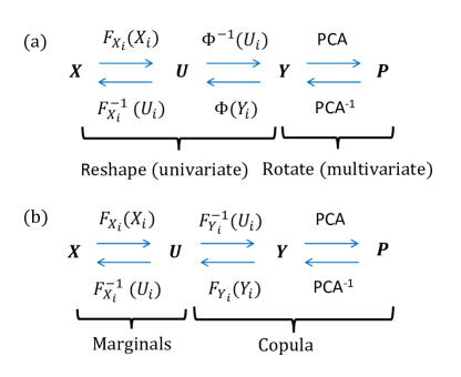
Figure 1: Modelling scheme for: (a) Principal Component Analysis based on normal scores, and for: (b) a general Principal Component Copula.

The third step is to apply PCA to the transformed variables $Y_{i}$. PCA is an orthogonal linear transformation, such that the correlated normalized variables $Y_{i}$ are rewritten in terms of uncorrelated variables $P_{j}$. PCA achieves this transformation by decomposing the correlation matrix $\bm{\rho}_{\bm{Y}}$ of $\bm{Y}$ into the orthogonal matrix of eigenvectors $\bm{W}$ and the diagonal eigenvalue matrix $\bm{\Lambda}$, so that $\bm{\rho}_{\bm{Y}}=\bm{W}\bm{\Lambda}\bm{W}^{T}$. The rotation from risk factors to Principal Components is performed by $\bm{P}=\bm{Y}\bm{W}$. For the inverse transformation, it follows that $\bm{Y}=\bm{P}\bm{W}^{T}$. The eigenvectors (the columns of $\bm{W}$) are ordered with decreasing eigenvalues. The eigenvector belonging to the highest eigenvalue gives the weights $w_{i,1}$ for the first principal component (PC).

As a result, the original task of modelling the joint distribution of the risk factors $X_{i}$ can be rewritten in terms of modelling the joint distribution of the PCs $P_{j}$. No information is lost in transforming the variables from $\bm{X}$ to $\bm{P}$. The first two steps in going from $X_{i}$ to $Y_{i}$ involve univariate transformations to rescale or reshape the individual variables, while the last step involves PCA, which can be viewed as a rotation of the data. An important advantage of PCA is that it gives a non-parametric method to identify the most relevant directions in high-dimensional data sets in terms of variance. This makes it a convenient starting point for making further model choices, such as modelling the PCs as independent risk factors or reducing the dimensionality by keeping only the most important PCs. In financial return data, the first PC typically describes the parallel movement of market variables. The next PCs describe the most important collective modes of diversification.

If we read the scheme in Fig. 1 from right to left, we schematically obtain the required steps for simulation of stochastic variables $X_{i}$, starting from the data generating process of the PCs. If we read the modelling scheme of Fig. 1a from left to right, we schematically obtain the required steps for calibration of the PCA model, starting from the observed data. Although the PCs $P_{j}$ are obtained by a linear combination of standard normal variables $Y_{i}$, the PCs will not necessarily be normally distributed. This is because the variables $Y_{i}$ are strongly dependent in the cases of interest, and only the sum of independent normal variables is guaranteed to remain normally distributed. Conversely, we may consider the case where the PCs $P_{j}$ are modelled as independent, but not necessarily identically distributed. In general, the sum over independent variables will converge to a normal distribution under the conditions of the Lyapunov central limit theorem. For a sum over a finite number of PCs, there will not be convergence to the normal distribution for $Y_{i}$. In that case, we have that $U_{i}=\Phi(Y_{i})$ is not uniformly distributed. This formally prevents interpretation of the modelling scheme in Figure 1a as a copula in first instance. As explained in Section 3, we use the scheme of Fig. 1a mainly for model exploration and initiation.

2.3 Copulas

An important advantage of a copula is that the modelling of the marginal distributions is separated from the modelling of the dependence structure. In general, the joint distribution function $F_{\bm{Y}}(y_{1},...,y_{d})$ for the stochastic vector $\mathbf{Y}$ can be expressed as $F_{\mathbf{Y}}(y_{1},...,y_{d})=C_{\mathbf{Y}}(F_{Y_{1}}(y_{1}),...,F_{Y_{d}}(y_{d}))$, with $F_{Y_{i}}$ the marginal distribution functions and $C_{\mathbf{Y}}(u_{1},...,u_{d})$ the copula. If the marginal distributions are continuous, then the copula is unique, which is the setting of relevance to our applications. Moreover, we have that $C_{\mathbf{Y}}(u_{1},...,u_{d})=F_{\mathbf{Y}}(F^{-1}_{Y_{1}}(u_{1}),...,F^{-1}_{Y_{d}}(u_{d}))$. This allows us to evolve the modelling scheme of Figure 1a into a Principal Component Copula (PCC). To this end, we show a slightly altered modelling scheme in Figure 1b. In order to ensure that $U_{i}$ is in general uniformly distributed, we apply $F^{-1}_{Y_{i}}$ in the second step. In general, this will not be the standard normal distribution $\Phi^{-1}$, because we allow the distribution $F^{-1}_{Y_{i}}$ to follow from any number of PCs $P_{j}$ with general distributions. The last two steps in the scheme of Figure 1b define the PCC.

Definition 1.

Consider two $d$-dimensional row vectors $\bm{Y}$ and $\bm{P}$ that are related to each other through the linear transformation $\bm{Y}=\bm{PW}^{T}$ with $\bm{W}$ an orthogonal matrix of eigenvectors from the correlation matrix $\bm{\rho}_{\bm{Y}}$. Let $F_{\bm{P}}$ be the multivariate distribution function of the stochastic vector ${\bm{P}}$. A Principal Component Copula $C_{\bm{Y}}$ is defined as the implicit copula for $\bm{Y}$ that follows from $F_{\bm{P}}$ and the linear transformation $\bm{Y}=\bm{PW}^{T}$.

Without loss of generality for the copula and to avoid overspecification, we take the variables $Y_{i}$ to be standardized with $E[Y_{i}]=0$ and $\text{var}[Y_{i}]=1$. As a result, the first and second moments of $\bm{Y}$ are fixed by the linear correlation matrix $\bm{\rho}_{\bm{Y}}$. Using the spectral theorem, we can always make the decomposition $\bm{\rho}_{\bm{Y}}=\bm{W}\bm{\Lambda}\bm{W}^{T}$, with $\bm{\Lambda}$ the diagonal matrix of nonnegative eigenvalues. In component form, the linear transformations are given by:

$$P_{j}=\sum_{i=1}^{d}w_{i,j}Y_{i}\,\,\,\text{and}\,\,\,Y_{i}=\sum_{j=1}^{d}w^{T}_{j,i}P_{j}=\sum_{j=1}^{d}w_{i,j}P_{j}.$$ (1)

The expectation value of $P_{j}$ is given by $E[{P_{j}}]=0$ and the variance by $\text{var}[{P_{j}}]=\Lambda_{j,j}=\lambda_{j}$, respectively. The PCs are ranked based on their variance, so that $P_{1}$ has the highest variance $\lambda_{1}$. If we specify the data generating process for the stochastic vector ${\bm{P}}$ as defined by its continuous multivariate distribution function $F_{\bm{P}}$, then the distribution function $F_{\bm{Y}}$ is fully specified by the linear transformation of Eq. (1). The copula distribution function for the PCC is given by: $C_{\bm{Y}}(u_{1},...,u_{d})=F_{\bm{Y}}(F^{-1}_{Y_{1}}(u_{1}),...,F^{-1}_{Y_{d}}(u_{d}))$, and the copula density by:

$$c_{\bm{Y}}(u_{1},...,u_{d}) = \frac{f_{\bm{Y}}(F_{Y_{1}}^{-1}(u_{1}),...,F_{Y_{d}}^{-1}(u_{d}))}{f_{Y_{1}}(F_{Y_{1}}^{-1}(u_{1}))...f_{Y_{d}}(F_{Y_{d}}^{-1}(u_{d}))}$$ (2)

$$= \frac{f_{\bm{Y}}(y_{1},...,y_{d})}{f_{Y_{1}}(y_{1})...f_{Y_{d}}(y_{d})}.$$

This setup is general, since we have only introduced a rotation to the variables $\mathbf{P}$, but not yet made any assumptions on the joint distribution for the PCs $F_{\bm{P}}$ (except continuity). As a result, we also have not yet made concrete progress.

2.4 Independent Principal Component Copulas

Next, we define an independent Principal Component Copula (iPCC), which models the PCs $P_{j}$ as independent stochastic risk drivers. Whether this is an appropriate choice for the uncorrelated PCs, depends on the application. When independence is a valid choice, then the multivariate modelling task simplifies significantly.

Proposition 1.

Consider a $d$-dimensional iPCC with probability densities $f_{P_{j}}$ and characteristic functions $\phi_{P_{j}}$ for the PCs $P_{j}$. Then, the copula density $c_{\bm{Y}}(u_{1},...,u_{d})$ for the iPCC can be expressed in terms of $f_{P_{j}}$ and $\phi_{P_{j}}$ using only one-dimensional integrals and one-dimensional inversions.

Proof.

We start from Eq. (2). For the iPCC, we find:

$$f_{\mathbf{Y}}(y_{1},..,y_{d}) = f_{\mathbf{P}}(\mathbf{y}\cdot\mathbf{w}_{1},...,\mathbf{y}\cdot\mathbf{w}_{d})\lvert J\rvert$$ (3)

$$= f_{P_{1}}(\mathbf{y}\cdot\mathbf{w}_{1})...f_{P_{d}}(\mathbf{y}\cdot\mathbf{w}_{d}),$$

where $\mathbf{y}=[y_{1},...,y_{d}]$, $\mathbf{w}_{i}$ denotes column $i$ from $\mathbf{W}$ and $f_{P_{j}}$ denotes the probability density of $P_{j}$. In the second step, we used the independence of PCs and that the Jacobian determinant $J$ equals $\pm 1$ for an orthogonal transformation. Next, we use that the characteristic functions multiply under convolution of independent stochastic variables. Since the characteristic functions $\phi_{P_{j}}$ for the distributions of $P_{j}$ are specified, we can straightforwardly determine the characteristic function $\phi_{Y_{i}}$ for the marginal distributions of $Y_{i}$ as:

$$\phi_{Y_{i}}(t)=\prod_{j}\phi_{P_{j}}(w_{i,j}t).$$ (4)

As a result, the marginal probability density $f_{Y_{i}}$ can be determined by a single integral, namely:

$$f_{Y_{i}}(y)=\frac{1}{2\pi}\int_{-\infty}^{\infty}\phi_{Y_{i}}(t)e^{-itx}dt.$$ (5)

The same holds for the marginal distribution function $F_{Y_{i}}$ through the Gil-Pelaez theorem:

$$F_{Y_{i}}(y)=\frac{1}{2}-\frac{1}{\pi}\int_{0}^{\infty}\frac{{\rm Im}[e^{-itx}\phi_{Y_{i}}(t)]}{t}dt.$$ (6)

Substituting Eqs. (3)-(5) and the inverse $F_{Y_{i}}^{-1}(u_{i})$ of Eq. (6) into Eq. (2) gives the required result. ∎

The integrals in Eqs. (3)-(6) can be numerically evaluated very efficiently using the Fast Fourier Transform [11] or can be approximated highly accurately by the COS-method [12]. $F^{-1}_{Y_{i}}$ can be obtained by numerical inversion. Since we have derived the copula density for an iPCC based on Eqs. (2-6), and since we only need to evaluate 1$D$-integrals to determine the full copula density, $c(u_{1},...,u_{d})$, it is feasible to compute the full copula density in high dimensions. This is useful for example to perform maximum likelihood estimation (MLE). In Section 4, we give numerical examples. We only consider the iPCC in the remainder of this article.

Remark 1.

For a factor copula based on multiple factors with general distributions, we have that Eq. (3) does not apply, because it is based on a latent model structure, rather than a rotation. As a result, determining $f_{\mathbf{Y}}$ and $c(u_{1},...,u_{d})$ becomes more cumbersome, because it requires integrating over all the common factors.

We can parameterize the PCC $C_{\boldsymbol{\Lambda},\mathbf{W},\boldsymbol{\alpha}}$ by the eigenvalue parameters $\lambda_{j}$, describing the variance of the PCs, by the orthogonal matrix elements $w_{i,j}$ describing the linear transformation from $P_{j}$ to $Y_{i}$, and by possible shape parameters $\alpha_{j}$, which allow $P_{j}$ to be skewed or heavy-tailed. By definition of the PCC, we require the parameters $\lambda_{j}$ and $w_{i,j}$ to form a valid correlation matrix. This leads to restrictions on admissible parameter values for $\lambda_{j}$ and $w_{i,j}$, which can be cumbersome to keep track of while performing estimation in high dimensions. As a result, we may also prefer to parametrize a PCC by the correlation matrix $\boldsymbol{\rho}_{\mathbf{Y}}$ and the shape parameters $\boldsymbol{\alpha}$. In case the eigenvalues $\lambda_{j}$ are non-degenerate, the eigenvalue decomposition of $\boldsymbol{\rho}_{\mathbf{Y}}$ is unique up to the sign for the eigenvectors. In practice, it is common to enforce a sign convention, for example, that the largest eigenvector weight is taken to be positive.

In case of degenerate eigenvalues $\lambda_{j}$, the eigenvalue decomposition is only uniquely defined up to an orthogonal transformation in the degenerate subspace. In that case, the PCC cannot be uniquely defined in terms of $\boldsymbol{\rho}_{\mathbf{Y}}$. An important exception is when the PCs corresponding to degenerate eigenvalues are modelled by a normal distribution. In that case, an orthogonal transformation does not change the distribution of the variables in the degenerate subspace and the copula distribution function $C_{\boldsymbol{\rho}_{\mathbf{Y}},\boldsymbol{\alpha}}$ remains the same.

In high-dimensional financial applications, we have that the eigenvalue spectrum typically consists of a (few) large distinct eigenvalue(s) and a dense set of smaller eigenvalues [19]. The first components determine the collective movement(s) of the market and are also the relevant components in generating tail dependence. The smaller eigenvalues typically do not differ from the spectrum that describes random noise [19]. Therefore, it is natural to consider PCCs that assign a more detailed model structure to the first PC(s), while the higher PCs are modelled with less detail, for example with a Gaussian distribution. Next, we give a concrete example of such a copula.

2.4.1 Hyperbolic-Normal iPCC

We introduce the Hyperbolic-Normal iPCC, for which we derive the tail dependence properties analytically. We start by considering the two-dimensional case. Suppose a positive linear correlation $\rho$ between the risk factors $Y_{i}$, such that $0<\rho<1$, and apply PCA to the correlation matrix of $\mathbf{Y}$. The first PC weight vector is then the parallel movement of the risk variables $\mathbf{w}_{1}=[1,1]^{T}/\sqrt{2}$, while the second PC weight vector is the anti-parallel movement $\mathbf{w}_{2}=[1,-1]^{T}/\sqrt{2}$. A negative correlation would cause the anti-parallel vector to be the first PC. Moreover, we have $\lambda_{2}=d-\lambda_{1}$ with $d=2$. So, we can equivalently parametrize the iPCC by either $\rho$ or $\lambda_{1}$.

Next, we consider the hyperbolic distribution with the following probability density $f_{X}$ for the stochastic variable $X\sim{\rm HB}(\alpha,\beta,\mu,\delta)$:

$$f_{X}(x)=\frac{\gamma}{2\alpha\delta K_{1}(\delta\gamma)}e^{-\alpha\sqrt{\delta^{2}+(x-\mu)^{2}}+\beta(x-\mu)},$$ (7)

where $\gamma=\sqrt{\alpha^{2}-\beta^{2}}$ and $K_{\nu}$ is a modified Bessel function of the second kind, $\mu$ is a location parameter, $\delta$ is a scale parameter, $\alpha+\beta$ describes the lower tail, and $\alpha-\beta$ the upper tail. We specify the characteristic function for the generalized hyperbolic distribution, from which the hyperbolic distribution is obtained by using $\lambda=1$:

$$\phi_{X}(t)=\frac{e^{i\mu t}\gamma^{\lambda}}{(\alpha^{2}-(\beta+it)^{2})^{\lambda/2}}\frac{K_{\lambda}\left(\delta\sqrt{\alpha^{2}-(\beta+it)^{2}}\right)}{K_{\lambda}(\delta\gamma)}.$$ (8)

The expressions for the mean and standard deviation of the hyperbolic distribution are known analytically. Therefore, we can choose parameters $\mu$ and $\delta$ such that $P_{1}$ is hyperbolically distributed with mean zero and variance $\lambda_{1}$. The second PC is taken to be normally distributed as $P_{2}\sim N(0,\sigma)$ with $\sigma=\sqrt{d-\lambda_{1}}$.

The hyperbolic distribution can be skewed and has heavier tails than the normal distribution. Consequently, we obtain asymmetric tail dependence for downward and upward shocks. This property is desired when constructing a realistic copula for financial returns. We prove the following proposition for the two-dimensional hyperbolic-normal copula $C^{HN}_{\lambda_{1},\alpha,\beta}(u_{1},u_{2})$.

Proposition 2.

Consider two independent PCs that are modelled with the hyperbolic distribution and the normal distribution: $P_{1}\sim{\rm Hyperbolic}(\alpha,\beta,\delta,\mu)$ and $P_{2}\sim{\rm N}(0,\sigma)$. Consider the risk factors $Y_{1}=(P_{1}+P_{2})/\sqrt{2}$ and $Y_{2}=(P_{1}-P_{2})/\sqrt{2}$. Then, the copula of $Y_{1}$ and $Y_{2}$ has a tail dependence parameter given by $\eta_{l}=2\Phi(-(\alpha+\beta)\sigma)$.

Proof.

We start by noting that the lower tail of $f_{P_{1}}$ from Eq. (7) is governed by:

$$\lim_{x\rightarrow-\infty}f_{P_{1}}(x)e^{-(\alpha+\beta)x}=\frac{\gamma}{2\alpha\delta K_{1}(\delta\gamma)}.$$ (9)

This means that in the lower tail, we can use that $f_{P_{1}}(x)\propto e^{(\alpha+\beta)x}$. We proceed by evaluating the general expression for the (lower) tail dependence coefficient $\lambda_{l}$:

$$\eta_{l} = \lim_{q\downarrow 0}P(U_{1}<q\lvert U_{2}<q)$$ (10)

$$= \lim_{y_{q}\rightarrow-\infty}2P(Y_{1}<y_{q}|Y_{2}=y_{q})$$

$$= \lim_{y_{q}\rightarrow-\infty}\frac{2\int_{-\infty}^{y_{q}}f_{Y_{1},Y_{2}}(y_{1},y_{q})dy_{1}}{f_{Y_{2}}(y_{q})}$$

$$= \lim_{y_{q}\rightarrow-\infty}\frac{2\int_{-\infty}^{y_{q}}f_{P_{1}}\left(\frac{y_{q}+y_{1}}{\sqrt{2}}\right)f_{P_{2}}\left(\frac{y_{q}-y_{1}}{\sqrt{2}}\right)dy_{1}}{\int_{-\infty}^{\infty}\sqrt{2}f_{P_{1}}(p_{1})f_{P_{2}}(\sqrt{2}y_{q}-p_{1})dp_{1}}$$

$$= \lim_{y_{q}\rightarrow-\infty}\frac{2\int_{-\infty}^{y_{q}}e^{(\alpha+\beta)(y_{1}+y_{q})/\sqrt{2}}e^{-(y_{1}-y_{q})^{2}/(4\sigma^{2})}dy_{1}}{\sqrt{2}\int_{-\infty}^{\infty}e^{(\alpha+\beta)p_{1}}e^{-(p_{1}-\sqrt{2}y_{q})^{2}/(2\sigma^{2})}dp_{1}}$$

$$= 2\Phi(-(\alpha+\beta)\sigma).$$

∎

The tail parameter $\eta_{l}$ approaches 1, when $(\alpha+\beta)$ goes to zero. This is expected because $P_{1}$ has a fatter lower tail, when $(\alpha+\beta)$ is smaller. Similarly, we can show that the upper tail dependence parameter is given by $\eta_{u}=2\Phi(-(\alpha-\beta)\sigma)$. We have thus constructed a copula with different upper and lower tail dependence, which can take any value between zero and one. This copula is based on two well-known distributions in the financial literature. The common factor that drives the dependence of the joint downward shocks is skewed and leptokurtic, while the higher-order factor is based on the normal distribution. Therefore, the additional complexity in the copula is added where it will be needed. We will show in applications that this copula is readily generalized to high dimensions and that it performs well on historic market data.

Remark 2.

For an elliptical distribution, tail dependence is generated when the density generator is regularly varying (power tailed) [2]. For a PCC, we have shown that we can also generate tail dependence with exponentially tailed variables, since there is no elliptical symmetry assumed.

Remark 3.

We have specified the characteristic function for the generalized hyperbolic distribution in Eq. (8). This broader family encompasses popular distributions in finance such as the Student’s t-distribution and the variance-gamma distribution. Due to the analytic characteristic function and probability density, this broader family is directly included in our approach, giving flexibility in building various iPCCs and capturing tail dependence.

2.5 Simulation procedure

PCCs are convenient to simulate when the data generating process is specified. In case of the iPCC, the simulation procedure is to first sample from the PC distributions for $P_{j}$. The second step is to apply the linear transformation to obtain samples for the transformed risk factors $\bm{Y}=\bm{W}^{T}\bm{P}$. The third step is to apply $F_{Y_{i}}$ to obtain samples for the copula $\bm{U}$. There are two different numerical approaches to obtain $F_{Y_{i}}$. The first method is to use Eq. (6), which is the approach we prefer and apply in this article. The second method is noting that we can simulate as many observations for $Y_{i}$ as desired and therefore obtain an arbitrarily accurate simulation-based empirical distribution function $\hat{F}_{Y_{i}}$ for $Y_{i}$.

3 Estimation procedures

Next, we discuss the model selection and estimation of PCCs. We start with the exploration and initiation of the model following the scheme of Fig. 1a. The advantage of this scheme is that the first three steps can be performed directly on the data with elementary techniques and without a priori knowledge about the distributions for the PCs. For a new data set, it would be difficult to apply the scheme in Figure 1b directly, because it requires knowledge of $F_{Y_{i}}$, which depends on the distribution choices for $\bm{P}$.

The first step can be performed using standard procedures to fit a parametric univariate distribution function $F_{X_{i}}$, based on the historic data $x_{i,t}$ (inference-function for margins approach). Another possibility is to use the non-parametric empirical distribution function to arrive at the observations $u_{i,t}$ (pseudo-likelihood approach). The practical advantage of the second method is that the values of $u_{i,t}$ can immediately be obtained as $u_{i,t}={\rm rank}(x_{i,t})/(n+1)$, where ${\rm rank}(x_{i,t})$ denotes the observed rank of $x_{i,t}$ in the sample $x_{i,1},...,x_{i,n}$. The second step of Figure 1a is also readily performed by obtaining the normal scores $y_{i,t}=\Phi^{-1}(u_{i,t})$. The third step is to apply PCA by determining the eigenvalues and eigenvectors of the sample correlation matrix of $\bm{Y}$ and gather the results in the diagonal matrix $\bm{\Lambda}$ and orthonormal matrix $\bm{W}$. When $\bm{y}$ and $\bm{p}$ denote the matrices with observations $y_{i,t}$ and $p_{j,t}$, we have that $\bm{p}=\bm{W}\bm{y}$, This means that the observations $p_{j,t}$ are obtained from matrix multiplication of the normal scores.

We have now rescaled and rotated the data, while automatically detecting the most important directions in the normal scores. In case of a Gaussian copula, the scheme of Fig. 1a is consistent and we could proceed by estimating each $P_{j}$ independently with the normal distribution. If the copula is not Gaussian, then the PCs are either not normally distributed or not independent. Then, $Y_{i}$ is generally not normally distributed and we should use $F_{Y_{i}}$ instead of $\Phi$. For model exploration and selection, it remains relevant to study the properties of $\Phi^{-1}(u_{i})$ with Fig. 1a. Using normalized marginals is a popular method to visualize copulas, since deviations from the Gaussian copula, like asymmetry and tail dependence, can be spotted immediately.

In financial applications, the application of PCA on normal scores typically gives accurate initial values for $\bm{\Lambda}$ and $\bm{W}$ as starting point for more advanced estimation schemes. We give explicit examples in Section 4. The reason is that the main directions in the multivariate data cloud $\mathbf{Y}$ correspond to the eigenvectors with the largest eigenvalues in the correlation matrix. The first eigenvector and eigenvalue are most robust to changes in the shape of the cloud. Therefore, Fig. 1a is useful both for model exploration and for the initial values of the estimation schemes we discuss next.

3.1 Maximum likelihood estimation

The self-consistent scheme of Fig. 1b defines a copula for which we derived the copula density in Section 2.4. Next, we explain maximum likelihood estimation (MLE) of the iPCC. We start from the general log-likelihood based on the copula density from Eq. (2), which results in:

$$\ell = \sum_{t=1}^{n}{\rm ln}\,c(u_{1,t},...,u_{d,t};\boldsymbol{\theta})$$

$$= \sum_{t=1}^{n}{\rm ln}\,f_{\mathbf{Y}}(y_{1,t},...,y_{d,t};\boldsymbol{\theta})-\sum_{t=1,i=1}^{n,d}{\rm ln}\,f_{Y_{i}}(y_{i};\boldsymbol{\theta}).$$

Here, $y_{i,t}=F^{-1}_{Y_{i}}(u_{i,t};\boldsymbol{\theta})$, while $f_{\mathbf{Y}},f_{Y_{i}}$ and $F_{Y_{i}}$ are given by Eq. (3-6). The maximum likelihood estimator is given by:

$$\hat{\boldsymbol{\theta}}=\underset{\boldsymbol{\theta}\in\boldsymbol{\Theta}}{\rm arg\,\,max\,\,}\ell(\boldsymbol{\theta};u_{1,t},..,u_{d,t}).$$ (12)

MLEs have the desirable asymptotic properties of being consistent and efficient. The main challenge for the PCC is to find a fast and accurate way to determine the copula density and the loglikelihood in Eq. (3.1), which can consequently be used in optimization algorithms for Eq. (12). This we discuss next.

3.1.1 Numerical approach

In order to perform the optimization from Eq. (12), we need to determine Eq. (5) and (6) fast and reliably. It is possible to efficiently evaluate Eq. (5) and (6) numerically with the Fast Fourier Transform, which has been used for option pricing in the finance literature [11]. Another highly efficient method from the option pricing literature is the COS method [12], which is based on the following cosine expansion:

$$f_{Y_{i}}(y)\simeq\frac{c_{0}}{2}+\sum^{N_{c}}_{k=1}c_{k}\cos\left(k\pi\frac{y-a}{b-a}\right).$$ (13)

The expansion coefficients $c_{j}$ can be analytically expressed in terms of the characteristic function $\phi_{Y_{i}}$ from Eq. (4) as [12]:

$$c_{k}=\frac{2}{b-a}{\rm Re}\left[\phi_{Y_{i}}\left(\frac{k\pi}{b-a}\right)e^{-i\frac{ka\pi}{b-a}}\right].$$ (14)

For $F_{Y_{i}}$, a similar expansion in terms of sine functions can be performed:

$$F_{Y_{i}}(y)\simeq\frac{c_{0}}{2}(y-a)+\sum^{N_{c}}_{k=1}c_{k}\frac{b-a}{k\pi}\sin\left(k\pi\frac{y-a}{b-a}\right).$$ (15)

Because $Y_{i}$ has unit variance and because the COS method converges exponentially, we already find accurate results with the following choices: $a=-10,b=10$ and $N_{c}=100$. Having implemented the COS method, we can efficiently evaluate $f_{Y_{i}}(y_{i})$ and $F_{Y_{i}}(y_{i})$ on any coordinate grid. If we evaluate $F_{Y_{i}}(y_{i})=u_{i}$ on a sufficiently fine grid, we immediately also obtain $F^{-1}_{Y_{i}}(u_{i})=y_{i}$ on the same grid. Any other value for $F^{-1}_{Y_{i}}(u_{i})$ can be obtained by interpolation. There are also more refined methods available for sampling from an inverse distribution functions, such as stochastic collocation [21].

Next, the optimization of Eq. (12) is performed to obtain the ML estimates. We have introduced the notation $C_{\boldsymbol{\Lambda},\mathbf{W},\boldsymbol{\alpha}}$ for the PCC, because the eigenvalue decomposition of $\boldsymbol{\rho}_{\mathbf{Y}}$ is unique (up to a sign) when the eigenvalues $\lambda_{j}$ are distinct. The ML optimization is initialized with the linear correlation matrix of the normal scores $\Phi^{-1}(u_{i,t})$, which is the ML estimator for the correlation parameters of the Gaussian copula, and with plausible starting values of the shape parameters $\alpha_{j}$. Gradient descent is then employed to update the parameters $\boldsymbol{\rho}_{\mathbf{Y}}$ and $\alpha$. After each update of $\boldsymbol{\rho}_{\mathbf{Y}}$, we perform PCA to obtain $\boldsymbol{\Lambda}$ and $\mathbf{W}$. The correlation matrices can be guaranteed to be positive semi-definite, by requiring the eigenvalues of $\boldsymbol{\Lambda}$ to be nonnegative, or by parameterising the correlation matrix using the method described by [22].

Full ML optimization is mainly feasible in low dimensions, or when additional structure is applied to the correlation matrix, so that it can be parametrized in a parsimonious way. In higher dimensions, with no additional predefined model structure, the number of correlation parameters $d(d-1)/2$ quickly becomes very large for numerical optimization. In that case, we propose a different estimation scheme in the next section.

3.2 Generalized Method of Moments

Besides ML, another popular class of estimators is the generalized method of moments (GMM) [23]. It starts from a vector-valued function $\bm{g}(\bm{Y},\boldsymbol{\theta})$ with an expectation value of zero at the true parameter values $\boldsymbol{\theta}_{0}$. The expectation value of $\bm{g}$ can be estimated with the vector valued sample mean:

$$\hat{\bm{m}}(\bm{\theta})=\frac{1}{n}\sum_{t}\bm{g}(\bm{Y}_{t},\bm{\theta}).$$ (16)

The GMM estimator is then given by [23]:

$$\hat{\bm{\theta}}=\underset{\bm{\theta}\in\bm{\Theta}}{\rm arg\,\,min\,\,}\hat{m}(\bm{\theta})^{T}\bm{W}_{g}\hat{m}(\bm{\theta}).$$ (17)

Here, $\bm{W}_{g}$ is a positive semi-definite weight matrix. The GMM estimator has the desirable asymptotic properties of being consistent and normally distributed. A suitable choice of the matrix $\bm{W}_{g}$ leads to the most efficient estimator based on the moment conditions.

In high dimensions, it is preferable to estimate the many correlation parameters with a moment estimator and the fewer shape parameters with an ML estimator. This is indeed the common approach in finance when using a $t$-copula [2], where the correlation parameters are usually based on Kendall’s tau estimates and the shape parameter $\nu$ using ML. We develop a similar strategy for the PCC. First, we introduce the generalized moment equations for the scale parameters $\boldsymbol{\rho}_{\bm{Y}}$ and the shape parameters $\boldsymbol{\alpha}$, giving:

$$E[F_{Y_{i}}^{-1}(U_{i})F_{Y_{j}}^{-1}(U_{j})-\rho_{Y,i,j}] = 0$$

$$E[\nabla_{\bm{\alpha}}\ell(\bm{\rho}_{\bm{Y}},\bm{\alpha};U_{1},..,U_{d})] = 0$$ (18)

In the second line, we have written the ML estimator as a GMM condition. This shows that an estimator based on the generalized moment conditions in Eq. (18) can be viewed as a GMM estimator.

3.2.1 Numerical approach

Next, we explain how we numerically arrive at the solution of the GMM equations following from the conditions in Eq. (18). Note that $F_{Y_{i}}^{-1}$ depends itself on $\boldsymbol{\rho}_{\mathbf{Y}}$ and $\boldsymbol{\alpha}$, making the corresponding equations nonlinear. However, in the applications of our interest, we find this dependence to be relatively weak, so that an iterative procedure can be used. The iterative procedure initializes the correlation matrix $\hat{\rho}^{(0)}_{\bm{Y}}$ with the sample correlation of the normal scores $\Phi^{-1}(u_{i,t})$. Next, we decompose the correlation matrix into eigenvectors using PCA. In general, the following equality holds for the PCC:

$$\rho(F^{-1}_{Y_{i}}(U_{i}),F^{-1}_{Y_{j}}(U_{j}))=E[Y_{i}Y_{j}]=\sum_{k}\lambda_{k}w_{i,k}w_{k,j}.$$ (19)

Here we used that $E[Y_{i}]=0$ and that the PCs $P_{j}$ are uncorrelated. Having initialized the PC vectors, we can determine the shape parameters $\boldsymbol{\alpha}$ using ML. To this end, we use Eqs. (2-6) for the likelihood in combination with the COS method. An iterative algorithm can then solve the GMM equations, which we show in Algorithm 1.

Algorithm 1 Iterative algorithm to estimate the PCC with GMM

1. Initialize scale parameters $\hat{\bm{\rho}}^{(0)}_{\bm{Y}}$ using:

   $$\hat{\rho}^{(0)}_{\bm{Y},i,j}=\frac{1}{N}\sum_{t}\Phi^{-1}\left(u_{i,t}\right)\Phi^{-1}\left(u_{j,t}\right)$$

2. Perform PCA to obtain initial PC vector weights $\hat{w}_{i,j}^{(0)}$ and eigenvalues $\hat{\lambda}_{j}^{(0)}$

3. Initialize shape parameters using ML:

   $$\hat{\bm{\alpha}}^{(0)}=\underset{\bm{\alpha}}{\rm arg\,\,max\,\,}\ell(\bm{\alpha},\hat{\bm{W}}^{(0)},\hat{\bm{\Lambda}}^{(0)};u_{1,t},..,u_{d,t}).$$

4. For each recursion step $k=1,..,n_{r}$ update parameters with $\hat{F}^{(k-1)^{-1}}_{Y_{i}}(u_{i,t})=F^{-1}_{Y_{i}}\left(u_{i,t};\hat{\rho}^{(k-1)}_{\bm{Y}},\hat{\bm{\alpha}}^{(k-1)}\right)$:

   1. Update scale parameters (correlations) given shape parameters:

      $$\hat{\rho}^{(k)}_{\mathbf{Y},i,j}=\frac{1}{N}\sum_{t}\hat{F}^{(k-1)^{-1}}_{Y_{i}}\left(u_{i,t}\right)\hat{F}^{(k-1)^{-1}}_{Y_{i}}\left(u_{j,t}\right)$$

   2. Perform PCA to update vector weights $\hat{w}_{i,j}^{(k)}$ and eigenvalues $\hat{\lambda}_{j}^{(k)}$

   3. Update shape parameters given scale parameters using ML:

      $$\hat{\bm{\alpha}}^{(k)}=\underset{\bm{\alpha}}{\rm arg\,max\,}\ell(\bm{\alpha},\hat{\bm{W}}^{(k)},\hat{\bm{\Lambda}}^{(k)};u_{1,t},..,u_{d,t}).$$

5. Return estimated GMM parameters $\{\hat{\bm{\rho}}^{(n_{r})}_{\bm{Y}},\hat{\bm{\alpha}}^{(n_{r})}\}$

In order for the iterative algorithm to converge towards a fixed point, the usual conditions for contraction are required, i.e., that derivatives are smaller than one around the fixed point. In Section 4, we show that the algorithm performs very well in the situations of interest, namely when there are a few distinct first PC vectors with large eigenvalues that can have a nontrivial structure based on their shape parameters. In the studied examples, the large eigenvalues are found to be robust against changes in the shape parameters. As a result, the initialization steps already give accurate results, and only a few iteration steps are required to obtain the full solution.

3.2.2 Other moments

The generalized method of moments can also include other dependence measures. The conditional probability of joint quantile exceedance (CPJQE) is for downward movements defined as: $\eta_{q,i,j}=P[U_{i}\leq q\lvert U_{j}\leq q]$. Denoting $u_{i,t}=\hat{F}_{X_{i,t}}(x_{i,t})=\text{rank}(x_{i,t})/(n+1)$, the estimate for the joint quantile exceedance is obtained by:

$$\hat{\eta}_{q,i,j}=\frac{1}{nq}\sum_{t}I_{\{u_{i,t}\leq q,u_{j,t}\leq q\}}.$$ (20)

Similarly, for upward movements the CPJQE is based on $P[U_{i}>q\lvert U_{j}>q]$. The limit $q\rightarrow 0$ of $\eta_{q,i,j}$ is called the coefficient of lower tail dependence $\eta_{i,j}$. In case of the Gaussian copula, this coefficient equals zero, meaning that no tail dependence is generated.

When applying the GMM, we can use a general vector of dependence measures. Oh and Patton consider for example all rank correlations $\rho_{S,i,j}$, all upper pairwise quantile exceedance probabilities and lower pairwise quantile exceedance probabilities [7]. For the GMM, we require the expressions of the dependence measures in terms of the model parameters. Analytical expressions are typically not available so that either numerical integration or simulation should be used. Since factor copulas and PCCs are convenient to simulate, it is easy to generate many simulated copula observations and approximate the required model expectation values with the desired accuracy. This technique is called simulated method of moments, and it was developed for factor copulas by Patton and Oh [7].

Although the simulated method of moments is conceptually simple and generally applicable, it can still be numerically challenging to achieve convergence for large-scale models. So far, there have not been studies that have shown robust estimation of a large number of parameters (e.g. more than 50 or 100 parameters) with this technique. In the next section, we show that we obtain robust estimates with the method of Section 3.2.1 that applies PCA-based moment estimation for the (many) correlation parameters and MLE for the (few) shape parameters. As a concrete example, we perform an estimation in 100 dimensions with 4954 parameters and find that the robustness of the proposed algorithm remains intact with growing dimensionality, which is considered an attractive feature.

4 Applications

4.1 Simulation study

We study the developed PCC and its estimators first using simulated data and afterwards using historical financial return data. We start with simulation studies in low dimensions and in high dimensions to establish the performance of the proposed estimators in different situations.

4.1.1 Low-dimensional case

We perform first a simulation study for a three-dimensional iPCC as defined by the distribution function of $\bm{Y}$ that follows from the scheme of Fig. 1b. The stochastic variables $Y_{i}$ have a mean equal to zero and a variance equal to $1$. Therefore, there are three parameters $\{\rho_{12},\rho_{23},\rho_{13}\}$ that determine the first and second moments of $\bm{Y}$. By performing PCA, we obtain the eigenvector matrix $\bm{W}$ and eigenvalues $\bm{\Lambda}$. The data generating process for $\bm{Y}$ is given by the linear tranformation $\bm{Y}=\bm{P}\bm{W}^{T}$ and the following distributions for the PCs:

$$P_{j}\sim{\rm HB}(\alpha_{j},\beta_{j},\lambda_{j})\,\forall j\in\{1,2\},\,P_{3}\sim N(0,\lambda_{3})$$ (21)

Here, we have introduced the notation ${\rm HB}(\alpha_{j},\beta_{j},\lambda_{j})$ for a PC that has the hyperbolic distribution from Eq. (7), where $\mu$ and $\delta$ are taken such that the mean is equal to zero and the variance is equal to $\lambda_{j}$.

In Table 1, the parameters selected for the study are presented. The chosen parameters for the first two PC distributions give rise to skewness and tail dependence, due to the heavier tails of the hyperbolic distribution compared to the normal distribution. We simulate the copula by first sampling the PCs independently from the hyperbolic and normal distributions. Then, we rotate the simulated data using $\bm{Y}=\bm{P}\bm{W}^{T}$. Finally, we return $U_{i}=F_{Y_{i}}(Y_{i})$ for the simulated copula observations, where $F_{Y_{i}}(Y_{i})$ is determined from Eqs. (4), (6) and (15). With the chosen parameters, we find that the copula has the following lower tail dependence parameters among the risk pairs: $\eta_{1,2}=0.60$, $\eta_{1,3}=0.43$, $\eta_{2,3}=0.34$.

Table 1: Estimation results based on a simulation study for the PCC in 3 dimensions using 5000 simulated data points. The second column shows the true parameter values, the third column the MLEs, the fourth column the corresponding standard deviation based on 50 Monte Carlo replications of the estimation procedure, the fifth and sixth columns show the estimate and the standard deviation based on GMM using Algorithm 1.

ML GMM True Est. Std. Dev. Est. Std. Dev. $\rho_{12}$ 0.75 0.751 0.005 0.749 0.011 $\rho_{13}$ 0.5 0.498 0.011 0.497 0.018 $\rho_{23}$ 0.25 0.249 0.015 0.247 0.026 $\alpha_{1}$ 1.632 1.625 0.069 1.642 0.066 $\beta_{1}$ -0.816 -0.808 0.066 -0.820 0.064 $\alpha_{2}$ 2.409 2.427 0.152 2.424 0.165 $\beta_{2}$ 0.482 0.495 0.091 0.495 0.090

In the simulation study, 5000 copula observations are generated for the estimation. We first apply full MLE, and numerically optimize the likelihood for the 7 parameters $\rho_{i,j},\alpha_{j}$ and $\beta_{j}$. The eigenvector weights $w_{i,j}$ and the eigenvalues $\lambda_{j}$ for the PCs follow at each optimization step from the updated $\rho_{i,j}$. We also perform the estimation procedure with the iterative GMM approach of Algorithm 1. In Table 1, the results after 5 iterations are shown, which was found to be sufficient to achieve convergence.

In order to study the performance of the estimation procedure, 50 Monte Carlo replications of the full estimation procedure are generated and the mean and the standard deviation of the estimators are determined. From Table 1, we see that the MLEs perform well in terms of bias and standard errors, as expected. We compare the ML estimator with the GMM estimator of Algorithm 1, which combines self-consistent sample estimates for correlation parameters with ML for the shape parameters. Using Algorithm 1, the estimates are slightly biased after the initiation step, which is expected due to the misspecification when using $\Phi^{-1}(U_{i})$ for $Y_{i}$. However, the initiation step still provides a good starting point for the iterative process. The bias of the estimator disappears after only a few iterations. The estimation results with Algorithm 1 are seen to give limited performance loss compared to ML. This performance is in line with our expectations, because combinations of moment estimators for correlations and ML estimators for shape parameters are known to perform well in simpler cases, such as the $t$ copula [16]. The advantage of the hybrid GMM estimator compared to full ML is that it can be readily applied in high dimensions, as is shown next.

4.1.2 High-dimensional case

Having shown that the GMM estimation approach performs well in low dimensions, we turn to the high-dimensional case, and consider 100 dimensions. We consider again an iPCC, where the first two PCs are given a non-trivial shape generating skewness and tail dependence. The data generating process for the PCs is similar to Eq. (21) with the hyperbolic distribution for the first two PCs and we use $P_{j}\sim N(0,\lambda_{j})$ for $j>2$. In our stylized example, the correlation matrix has the following structure, generated by two main factors:

$$\rho_{Y_{i},Y_{j}}=\xi_{i}\xi_{j}+\gamma_{i}\gamma_{j}$$ (22)

Here, we use the following expressions for $i$ ranging from 1 to $d$:

$$\xi_{i}=\frac{2}{5}\left(1+e^{-i/d}\right),\quad\gamma_{i}=\frac{3}{5}\tanh(4i/d-2).$$ (23)

This parametrization leads to $d(d-1)/2$ different correlation parameters with values ranging from $0.10$ to $0.96$. We do not inform our estimation algorithm about the underlying parameter structure. Applying PCA gives the eigenvectors and eigenvalues of $\rho_{Y_{i},Y_{j}}$, where the first two PC vectors are shown in Fig. 2. These vectors are seen to describe a parallel shock and an anti-parallel shock in line with $\xi_{i}$ and $\gamma_{i}$. The first PCs have eigenvalues $\lambda_{1}=43.8$ and $\lambda_{2}=18.5$, respectively, which therefore explain 62% of the variance. All higher PCs have eigenvalues less than 1, so that they do not carry relevant information in this example. Note that the first PC vectors are not exactly the same as the factors $\xi_{i}$ and $\gamma_{i}$, because the PCs are normalized and perpendicular. It is our copula design choice to specify the data generating process in terms of PCs rather than latent factors.

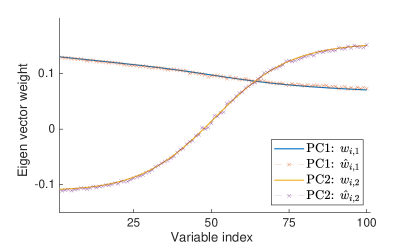
Figure 2: True eigenvector weights $w_{i,j}$ and estimated eigenvectors weights $\hat{w}_{i,j}$ for the first two Principal Components $j\in\{1,2\}$ as a function of the variable index $i\in\{1,...,100\}$. The differences are very small.

In the high-dimensional simulation study, again 5000 copula observations are generated for the estimation. We start with applying MLE only for the 4 shape parameters $\alpha_{j}$ and $\beta_{j}$, taking the true eigenvector weights $w_{i,j}$ and eigenvalues $\lambda_{j}$ as given. This hypothetical situation is used as performance reference. Next, the hybrid estimation procedure from Algorithm 1 is applied, which estimates all the 4950 correlation parameters and the 4 shape parameters jointly. Again 50 Monte Carlo replications of the full estimation procedure are generated to determine the performance of the estimators. In Table 2, the results for the four shape parameters using ML estimation and the results with Algorithm 1 are presented. We also show the results for the first two eigenvalues $\lambda_{j}$. The estimation result for the corresponding eigenvectors $\hat{w}_{i,j}$ are shown in Fig. 2, which reveals that the eigenvector estimates are very accurate.

Table 2: Estimation results based on a simulation study for the PCC in 100 dimensions using 5000 simulated data points. The second column shows the true parameter values, the third column the MLEs for only the shape parameters (using the true values for the other parameters) and the fourth column the corresponding standard deviations based on 50 Monte Carlo replications of the estimation procedure. The fifth and sixth columns show the estimate and the standard deviations based on GMM using Algorithm 1.

ML GMM True Est. Std. Dev. Est. Std. Dev. $\lambda_{1}$ 43.78 43.67 0.70 $\lambda_{2}$ 18.53 18.55 0.36 $\alpha_{1}$ 0.71 0.71 0.05 0.73 0.06 $\beta_{1}$ -0.47 -0.48 0.05 -0.49 0.05 $\alpha_{2}$ 0.94 0.95 0.12 0.94 0.13 $\beta_{2}$ 0.31 0.32 0.08 0.31 0.09

From Table 2, it is seen that the MLEs for the shape parameters perform well in terms of bias and standard errors, as expected, since the true eigenvector weights and eigenvalues were used. We compare these ML shape estimates with the hybrid GMM estimator of Algorithm 1. As in the low-dimensional case, the estimates have a small bias after the initiation step which disappears after only a few iterations. The estimation results of Algorithm 1 in the last columns are seen to give very similar performance for the shape parameters compared to the ML shape estimates, even though an additional 4950 correlation parameters are estimated. The hybrid GMM estimator of Algorithm 1 did not use any information on the underlying correlation structure. The algorithm was able to automatically detect the most important directions in the data using PCA and to estimate nontrivial distributions in these directions using ML. We observe that the algorithm works very well in high dimensions when the first PCs have large eigenvalues, so that the PC vectors can be robustly detected. Then, the algorithm avoids the curse of dimensionality, because the dimensions are reduced to only the most important PCs with non-trivial distributions. Note that our example is stylized but realistic. In financial markets, we also typically observe a (few) dominant factor(s) in terms of variance.

4.2 Case study

Next, we turn from simulated data to actual financial return data. We apply the developed methodology to weekly return data for 20 major stock indices around the world. The weekly data starts at 1 January 1998 and ends on 29 December 2022, resulting in 25 years of data with $n=1304$ weekly returns. Table 3 shows relevant summary statistics of the stock indices that are included in the analysis. The time series data of weekly logreturns $r_{i,t}$ for each index $i$ are filtered with the commonly used GARCH(1,1) model to account for volatility clustering:

$$r_{i,t} = \sigma_{i,t}x_{i,t},$$

$$\sigma^{2}_{i,t} = \omega_{G,i}+\alpha_{G,i}x^{2}_{i,t-1}+\beta_{G,i}\sigma^{2}_{i,t-1}.$$ (24)

We estimate the parameters $\mu_{G,i},\nu_{G,i},\omega_{G,i},\alpha_{G,i}$ and $\beta_{G,i}$ of the GARCH filter using quasi-maximum likelihood. For the distribution of the filtered residual returns $x_{i,t}$, we use the empirical distribution function, so that the pseudo-copula observations are obtained by $u_{i,t}=\text{rank}(x_{i,t})/(n+1)$.

Table 3: Stock indices that are included in the empirical analysis. The weekly standard deviation and the weekly worst-case logreturn are also shown.

Nr. Index Country Std dev (%) Min. (%) 1 DAX Germany 3.22 -21.23 2 FTSE 100 UK 2.40 -14.83 3 CAC 40 France 3.06 -20.52 4 FTSE MIB Italy 3.29 -20.22 5 IBEX 35 Spain 3.15 -18.08 6 AEX Netherlands 3.11 -18.08 7 ATX Austria 3.33 -34.64 8 HSI Hong Kong 3.26 -15.48 9 Nikkei 225 Japan 3.06 -21.12 10 STI Singapore 2.77 -15.51 11 Kospi South Korea 3.50 -18.17 12 Sensex India 3.24 -21.23 13 IDX Comp. Indonesia 3.28 -23.30 14 KLCI Maleysia 2.48 -15.30 15 SP 500 US 2.42 -16.45 16 TSX Comp. Canada 2.32 -19.68 17 Bovespa Brazil 4.01 -26.63 18 IPC Mexico 2.93 -19.44 19 All ord. Australia 2.01 -14.68 20 TA 125 Israel 2.59 -16.91

We start by comparing the performance of several copulas in the three-dimensional case, selecting the FTSE-100 ($i=2$), Nikkei-225 ($i=9$) and the S&P-500 ($i=15$) as three major stock indices, where we consider the Gaussian copula, the $t$ copula, and the Skew $t$ copula by Demarta and McNeil [16]. The Gaussian copula and the $t$ copula are most commonly used in practice at financial institutions. The Skew $t$ copula is an important extension due to its ability to capture asymmetry between up and down movements. Besides these normal mixture copulas, we also include two PCCs in the comparison. We choose the Hyperbolic-Normal PCC, where the first PC is modelled with the Hyperbolic distribution and the other PCs with the normal distribution. We also select the Skew $t$-$t$ PCC, where the first PC is modelled with the Skew $t$ distribution and the other PCs with the $t$ distribution, which is therefore similar to the factor copula studied by Patton and Oh [7]:

$$P_{1}\sim{\rm Skew}\,t(\nu,\gamma,\lambda_{1}),\quad P_{j}\sim t(\nu,\lambda_{j})\,\forall j>2.$$ (25)

Here, ${\rm Skew}\,t(\nu,\gamma,\lambda_{1})$ and $t(\nu,\lambda_{j})$ denote the Skew $t$ and $t$ distribution with degrees-of-freedom parameter $\nu$, asymmetry parameter $\gamma$, variance $\lambda_{j}$ and zero mean. Full MLE is performed for the five mentioned copulas.

The estimation results are shown in Table 4. To determine standard deviations of estimated parameters the bootstrap method was used [24]. This means that we have resampled the filtered historic data $x_{i,t}$ with replacement and reperformed MLE on 50 bootstrap samples. For the HB-N iPCC, we obtain a stronger downward tail than upward tail for the first PC due to the significantly negative value of $\hat{\beta}$. This results in pairwize downward tail dependence parameters between the stock indices given by $\hat{\eta}_{2,9}=0.31$, $\hat{\eta}_{2,15}=0.41$ and $\hat{\eta}_{9,15}=0.27$. The best performance of the copulas in terms of likelihood and BIC is obtained by the Skew $t$-$t$ PCC, followed by the Skew $t$ copula, and the HB-N PCC. These three copulas are able to capture asymmetric tail dependence.

Table 4: Estimation results for various copulas using 3-dimensional weekly return data (FTSE 100, Nikkei 225 and S&P 500). The estimates for the copula parameters are presented, as well as the loglikelihood $\ell$ and the BIC. Bootstrap standard deviations of estimates are shown in parentheses.

Gauss Student $t$ Skew $t$ HB-N PCC Skew $t$-$t$ PCC $\hat{\rho}_{12}$ 0.55 0.55 0.43 0.57 0.56 (0.02) (0.02) (0.06) (0.03) (0.02) $\hat{\rho}_{13}$ 0.69 0.69 0.61 0.68 0.70 (0.01) (0.02) (0.04) (0.02) (0.01) $\hat{\rho}_{23}$ 0.53 0.53 0.40 0.52 0.55 (0.02) (0.02) (0.06) (0.03) (0.02) $\hat{\nu}$ 15.1 17.7 23.0 (8.5) (5.2) (9.8) $\hat{\gamma}$ -1.45 -1.65 (0.5) (1.0) $\hat{\alpha}$ 2.55 (0.18) $\hat{\beta}$ -1.18 (0.28) $\ell$ 686.4 695.4 718.5 712.9 721.0 BIC -1351 -1362 -1401 -1390 - 1406

Next, we turn to the full 20-dimensional model, where all stock indices of Table 3 are included. Having performed the GARCH-filter and the rank-based transform to pseudo-copula observations $u_{i,t}$, we proceed with the inverse normal transform $\Phi^{-1}(u_{i,t})$ and apply PCA. The resulting eigenvector weights are shown in Fig. 3. The variable indices have the same order as in Table 3. The first PC-vector captures the movement of the market as a whole, since all vector weights $\hat{w}_{i,1}$ have the same sign. The Western European and the North American indices are found to have the strongest co-movement with the market, while the Maleysian and the Indonesian indices have the weakest co-movement.

The second PC gives the most important mode of diversification. In our case study, it describes the movement of the Asian indices ($i=8$-14) compared to the Western indices ($i=1$-7, 15-16). The other indices ($i=17$-20) have small vector weights $\hat{w}_{i,2}$, signalling that they fall geographically or economically in between these two categories. Note also that the Japanese index ($i=9$) has a smaller vector weight $\hat{w}_{9,2}$ than the other Asian indices in the second PC, meaning that it moves less strongly opposite to the Western indices. We can therefore interpret the Japanese index as the most western index of the included Asian indices. It is seen as a strong point of the methodology that detailed, yet plausible, economic effects are automatically captured by the copula. The third PC mainly describes the joint movement of the American indices ($i=15$-18) relative to other indices, where especially the additional variance of the two Latin-American indices ($i=17,18$) is captured. We conclude that the dominant collective movements of the market obtained by PCA have clear economic interpretations. It is an important property for a (regulatory) capital model that the key risk drivers are explainable.

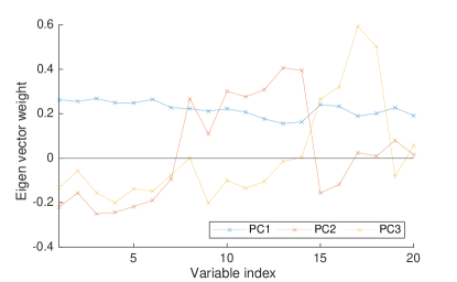
Figure 3: Estimated eigenvectors weights $\hat{w}_{i,j}$ for the first three Principal Components $j\in\{1,2,3\}$ as a function of the variable index $i\in\{1,...,20\}$.

We use the obtained eigenvectors and eigenvalues as initialisation for Algorithm 1 to obtain the full iterative solution of the GMM estimator for the Hyperbolic-Normal PCC. The procedure converges within a few iterations. The iterative solutions for the vector weights $\hat{w}_{i,j}$ of the first PCs hardly deviate from the initial weights in Fig. 3, revealing that the most important eigenvectors are robust to changes in shape parameters. The behavior of the estimated HB-N PCC is visualized using the steps of Fig. 1b. The result is shown in Fig. 4. Although the model is 20-dimensional, we select the FTSE-100 and the S&P-500 indices for visualization at index level. The first plot shows the historically observed logreturns after applying the GARCH-filter ($x_{i,t}$). The empirical distribution functions $\hat{F}_{X_{i}}$ are used to obtain the second plot, which shows the historical (pseudo) copula observations ($u_{i,t}$). The estimated inverse marginal distribution functions $\hat{F}^{-1}_{Y_{i}}$ are used to obtain the third plot, which shows the historical reshaped risk factors $(y_{i,t})$. The PCA-based rotation is used to obtain the right plot, which shows the historical PC observations ($p_{j,t}$ for $j=1,2$).

For the simulations, we show the steps in the opposite direction, starting from simulating all PCs $\tilde{p}_{j,t}$ by sampling from the hyperbolic and normal distributions, subsequently applying the (inverse) PCA-based rotation to obtain the simulated reshaped risk factors $\tilde{y}_{i,t}$. The estimated marginal distribution functions $\hat{F}_{Y_{i}}$ are used to obtain the simulated copula observations $\tilde{u}_{i,t}$, and finally the inverse empirical distribution functions $\hat{F}^{-1}_{X_{i}}$ are used to simulate the filtered logreturns $\tilde{x}_{i,t}$. Fig. 4 shows that we can visualize and assess the performance at each layer of the model. This holds in particular for the first two PCs, which are the core risk drivers that explain about 65% of the total variance. Fig. 4 also shows that the reshaped observations $y_{i,t}$ have fewer outliers than the initial observations $x_{i,t}$, which is beneficial for PCA.

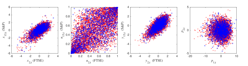
Figure 4: Visualization of the model layers from Fig. 1b based on historical observations (blue dots) and on simulations from the estimated Hyperbolic-Normal PCC (red dots). Although the data and the model are 20-dimensional, the FTSE-100 and the S&P-500 indices are used for visualization at index level. The left plot shows the (filtered) logreturn observations ($x_{i,t}$), the second plot shows the (pseudo-)copula observations ($u_{i,t}$), the third plot shows reshaped risk factor observations ($y_{i,t}$) and the right plot shows the PC observations for the first two PCs ($p_{j,t}$).

Table 5: Estimation results for the 20-dimensional weekly return data using the indices from Table 3. The estimates for the copula shape parameters are presented, as well as the loglikelihood $\ell$. Bootstrap standard deviations of estimates are shown in parentheses. We also show the average pairwize CPJQE $\bar{\eta}_{q}$ over all pairs with $q=0.05$, and the total CPJQE for all indices $\hat{\eta}^{\rm tot}_{q}$ with $q=0.2$.

Gauss Student $t$ Skew $t$ HB-N Skew $t$-$t$ History $\hat{\nu}$ 14.6 13.5 15.0 (1.4) (2.1) (2.5) $\hat{\gamma}$ -2.75 -1.07 (0.30) (0.32) $\hat{\alpha}$ 1.29 (0.29) $\hat{\alpha}$ -0.68 (0.22) $\ell$ 10,531 10,969 11,065 10,727 10,843 $\bar{\eta}_{q}$ 0.335 0.368 0.415 0.419 0.488 0.412 $\hat{\eta}^{\rm tot}_{q}$ 0.014 0.019 0.027 0.041 0.077 0.058

In Table 5, the estimation results for the 20-dimensional copulas are shown. We only show the estimated shape parameters. The Gaussian and the $t$ copula are straightforward to estimate in high dimensions [2]. This is not the case for the Skew $t$ copula, which is a normal mixture copula that in general depends on a vector of asymmetry parameters $\bm{\gamma}$. Our approach is to align this vector with the first eigenvector of the correlation or covariance matrix, so that $\bm{\gamma}=\gamma\bm{w}_{1}$. With this choice, the eigenvectors of the covariance matrix remain unchanged for a normal mixture copula upon increasing $\gamma$ and $\nu$. Therefore, we freeze the eigenvectors, which simplifies the ML estimation significantly. Moreover, the first PC vector is also the most important direction for including skewness. For the Hyperbolic-Normal (HB-N) PCC and for the Skew $t$-$t$ PCC, Algorithm 1 is used for estimation. Because the characteristic functions for all distributions in the PCCs are known, we can apply Eqs. (13) and (15) to obtain the distribution and density functions at the required accuracy. To determine the standard deviations of the estimated parameters the bootstrap method was used, where Algorithm 1 was reperformed for 50 bootstrap samples.

From Table 5, it becomes clear that the Gaussian copula has the lowest likelihood. Significant improvement is obtained upon generalizing to the $t$ copula to include tail dependence and upon generalizing to the Skew $t$ copula to allow for asymmetry between joint up and down movements. For a capital model, not only the likelihood, but also tail dependence measures are important in assessing the adequacy of the copula. For pairwise dependence in the tail, the CPJQE ($\hat{\eta}_{q,i,j}$) in Eq. (20) measures simultaneous exceedances of extreme quantiles. In order to capture all index pairs in a single measure, we consider the averaged CPJQE ($\bar{\eta}_{q}$) over all pairs:

$$\bar{\eta}_{q}=\frac{2}{d(d-1)}\sum^{d}_{i=1,j>i}\hat{\eta}_{q,i,j}.$$ (26)

In Table 5, $q=0.05$ is used for $\bar{\eta}_{q}$. At this quantile, we are quite far in the lower tail, but still have typically around 25 joint exceedances out of 1304 observations for each index pair, allowing for reasonably stable estimates. It can be seen that, historically, the averaged pairwize CPJQE $\bar{\eta}_{0.05}$ has been estimated at 0.41. For the copula models, $10^{6}$ simulations are employed to accurately determine $\eta_{q,i,j}$ and $\bar{\eta}_{q}$. The Gaussian copula and the Student $t$ copula are seen to have significantly lower pairwise dependence in the tail. The Skew $t$ and the HB-N PCC are very accurate in capturing pairwize tail dependence on average. The Skew $t$-$t$ PCC leads to a more conservative dependence in the tail than historically observed.

Another measure of tail dependence is the CPJQE for all indices combined. This quantity measures the probability that all indices exceed a given quantile $q$ simultaneously (given that the first index exceeds the quantile):

$$\hat{\eta}^{\rm tot}_{q}=\frac{1}{nq}\sum_{t}I_{\{u_{1,t}\leq q,u_{2,t}\leq q,...,u_{d,t}\leq q\}}.$$ (27)

In Table 5, $q=0.20$ is used for $\hat{\eta}^{\rm tot}_{q}$. Historically, we have observed 15 exceedances of this quantile for all indices simultaneously out of 1304 observations. For the copula models, simulations are again employed to accurately determine $\eta^{\rm tot}_{q}$ per model. The Gaussian copula, the Student $t$ copula, and the Skew $t$ copula are seen to give significantly lower values of the total CPJQE $\hat{\eta}^{\rm tot}_{q}$ than historically observed. The HB-N PCC and the Skew $t$ PCC perform much better in capturing this measure of systemic risk. These conclusions are in line with the observations of Patton and Oh [7], who considered other measures of systemic risk to conclude that copulas with common factors outperform other popular copulas in finance. We extend our analysis in Fig. 5, where we show the pairwize CPJQE for the FTSE-100 index and the S&P-500 index as a function of the quantile $q$. We also show the total CPJQE for all indices $\hat{\eta}^{\rm tot}_{q}$. The confidence intervals for the empirical estimates are again determined using the bootstrap method. In particular for the aggregate dependence metric $\hat{\eta}^{\rm tot}_{q}$ in the right figure, we find that the iPCCs lead to better agreement with historical data than the normal mixture copulas.

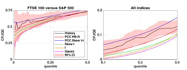
Figure 5: Upper: pairwize CPJQE-plot $\hat{\eta}_{q,i,j}$ using historical weekly logreturn observations for the FTSE-100 index and the S&P-500 index as a function of the quantile $q$ (black line). For the same index pair, the pairwize CPJQE-plots are also shown using simulations from the estimated (20-dimensional) Gaussian copula, $t$ copula, Skew $t$ copula, PCC HB-N and PCC Skew $t$-$t$. Confidence intervals are given based on bootstrapping the historical data and showing the 2.5% and 97.5% quantiles of empirical estimates. Lower: joint CPJQE-plot $\hat{\eta}^{\rm tot}_{q}$ using historical weekly logreturn observations for all 20 indices as a function of the quantile $q$ (black line). The combined CPJQE-plots are also shown using simulations from the estimated (20-dimensional) copulae. Confidence intervals are again given based on bootstrapping the historical data.

To further analyze this observation, we perform a binomial test for modelled exceedance probabilities against observed exceedance frequencies at $q=0.1$ and $q=0.2$. Historically, there have been 5 observed weeks where all indices simultaneously experienced at least a 90% worst-case loss ($q=0.1$), and there have been 15 observed weeks with at least a simultaneous 80% worst-case loss ($q=0.2$). In case of the Gaussian copula, the $p$-values from the binomial test for these observations are $1.2\cdot 10^{-5}$ and $1.1\cdot 10^{-6}$, respectively. For the $t$ copula, the $p$-values are $3\cdot 10^{-4}$ and $4\cdot 10^{-5}$. For the Skew $t$ copula, the $p$-values are $0.02$ and $0.002$. The normal mixture copulas are therefore rejected by one-sided binomial tests at a significance level of 5%. In case of the HB-N iPCC copula, we find that the $p$-values of the binomial test are $0.10$ and $0.08$. For the Skew $t$-$t$ iPCC, the $p$-values are $0.76$ and $0.85$. As a result, both PCCs both pass the test for aggregate dependence at a significance level of 5%. The improved ability of the iPCC to capture aggregate dependence in the tail is of importance to capital modelling.

Remark 4.

In a (regulatory) capital model, it may be preferable to have a through-the-cycle (or unconditional) capital rather than a point-in-time (or conditional) capital. The GARCH-filter in principle leads to a point-in-time and procyclical capital. When this is not desired, then it is a consideration to omit the GARCH-filter, or to replace the time-dependent volatility with a through-the-cycle estimate. Moreover, in a capital model it can be beneficial to have only a limited number of risk drivers for explainability and stability. This is achieved in the PCC by reducing the number of PCs that are included in the copula.

5 Conclusion

In this article, we have introduced the class of Principal Component Copulas, which combines the strong points of copula-based models with PCA-based models. The PCC is conceptually related to the class of factor copulas, since both copula types are able to capture the main drivers for diversification in high-dimensional data. Technically, the PCC is different from a factor copula, because it is formally based on reshaping and rotating the data, and not on imposing a latent model structure for a factor copula. We have shown that this gives rise to practical and technical advantages. First of all, we have been able to automatically detect the most relevant joint directions in high-dimensional copula data without requiring a priori knowledge of the underlying model. Secondly, we have represented the full copula density for an iPCC in terms of characteristic functions. This has allowed us to compute the copula density in arbitrarily high dimensions, while resolving only one-dimensional integrals that can be evaluated very efficiently. Thirdly, we have developed an algorithm that is designed to estimate a large number of scale parameters using the GMM and a selected number of shape parameters based on ML. This algorithm avoids the curse of dimensionality, leading to robust estimation of very large models in terms of dimensions and parameters.

Our techniques have been applied to financial return data, where we have shown that PCCs are able to identify collective movements in the market, while providing clear economic interpretations of the corresponding key risk drivers. By modelling the first PC with a distribution that is skewed and leptokurtic, we are able to add complexity and flexibility to the copula where it is needed. We have considered a binomial test for high-dimensional dependence of downward shocks, for which most commonly used copulas in finance fail, even when they capture pairwize tail dependence. The PCCs lead to significant improvements in passing this aggregate dependence test, so that we consider such copulas to be promising for capital modelling.

So far, we have limited ourselves to modelling the PCs as independent. For the iPCC, it is a direction for future research to consider Independent Component Analysis (ICA) to detect the independent directions of the components. Another direction for future research is to relax the assumption of independence, and to study PCCs where the higher PCs are allowed to have conditional dependence on the first PC(s). Because PCA and copula-based techniques are applicable to a wide range of data sets, it would be interesting to research the performance of the PCC on other data sets as well.

References

- [1] Cherubini U, Luciano E, Vecchiato W. (2004) Copula Methods in Finance. Wiley, New York.
- [2] McNeil AJ, Frey R, Embrechts P (2005) Quantitative Risk Management. Princeton University Press, Princeton.
- [3] Hull J, White A (2004) Valuation of a CDO and an nth to Default CDS Without Monte Carlo Simulation. Journal of Derivatives, 12: 8–23.
- [4] Andersen L, Sidenius J (2004) Extensions to the Gaussian Copula: Random Recovery and Random Factor Loadings. Journal of Credit Risk, 1: 29–70.
- [5] Krupskii P, Joe H (2013), Factor copula models for multivariate data. Journal of Multivariate Analysis, 120: 85-101.
- [6] Creal DD, Tsay RS (2015), High dimensional dynamic stochastic copula models. Journal of Econometrics, 189: 335-345.
- [7] Oh DH, Patton AJ (2017) Modeling dependence in high dimensions with factor copulas. Journal of Business & Economic Statistics, 35: 139-154.
- [8] Opschoor A, Lucas A, Barra I, Van Dijk D (2020) Closed-form multi-factor copula models with observation-driven dynamic factor loadings. Journal of Business & Economic Statistics, 39: 1066-1079.
- [9] Duan F, Manner H, Wied D (2022) Model and Moment Selection in Factor Copula Models. Journal of Financial Econometrics, 20: 45–75.
- [10] Oh DH, Patton AJ (2023) Dynamic Factor Copula Models with Estimated Cluster Assignments. Journal of Econometrics, 237: 105374.
- [11] Carr P, Madan D (1999) Option valuation using the fast Fourier transform. Journal of Computational Finance,2:61–73.
- [12] Fang F, Oosterlee CW (2009), A novel pricing method for European options based on Fourier-cosine series expansions. SIAM Journal on Scientific Computing, 31: 826-848.
- [13] Nelsen RB (2006) An Introduction to Copulas. Springer, New York.
- [14] Joe H (2014) Dependence Modeling with Copulas. Chapman & Hall, London.
- [15] Li DX (2000) On Default Correlation: A Copula Function Approach. Journal of Fixed Income, 9: 43–54.
- [16] Demarta S, McNeil AJ (2005) The t Copula and Related Copulas. International Statistical Review, 73: 111-129.
- [17] Aas K, et al. (2009) Pair-copula constructions of multiple dependence. Insurance: Mathematics and Economics, 44: 182-198
- [18] Stock JH, MW Watson (2002) Forecasting using principal components from a large number of predictors. Journal of the American statistical association, 97: 1167-1179.
- [19] Bun J, Bouchaud JP, Potters M (2017) Cleaning large correlation matrices: tools from random matrix theory. Physics Reports, 666: 1-109.
- [20] Hult H and Lindskog F (2002) Multivariate extremes, aggregation and dependence in elliptical distributions. Advances in Applied probability, 34: 587-608
- [21] Grzelak LA, Witteveen JAS, Suárez-Taboada M and Oosterlee CW (2019) The stochastic collocation Monte Carlo sampler: highly efficient sampling from ‘expensive’ distributions. Quantitative Finance, 19: 339-356.
- [22] Archakov I and Hansen PR (2021) A New Parametrization of Correlation Matrices. Econometrica, 89: 1699-1715.
- [23] Hansen LP (1982) Large sample properties of generalized method of moments estimators, Econometrica, 50: 1029-1054.
- [24] Efron B, Tibshirani RJ (1994), An Introduction to the Bootstrap. CRC Press, Boca Raton.