New physics interpretations for nonstandard values of $h\to Z\gamma$

Abstract

Current measurement of the $h\to Z\gamma$ signal strength invite us to speculate about possible new physics interactions that exclusively affect $\mu_{Z\gamma}$ without altering the other signal strengths. Additional consideration of tree-unitarity enables us to correlate the nonstandard values of $\mu_{Z\gamma}$ with an upper limit on the scale of new physics. We find that even when $\mu_{Z\gamma}$ deviates from the SM value by only $20\%$, the scale of new physics should be well within the reach of the LHC.

The loop-induced decay modes of the Higgs boson ($h$) have been impactful in many different aspects of Higgs physics. The decay $h\to\gamma\gamma$, in particular, played a pivotal role in the discovery of the Higgs boson[1, 2]. Such loop-induced Higgs couplings have also been proved useful in sensing the presence of new physics beyond the Standard Model (BSM) through new loop contributions arising from additional nonstandard particles[3]. This is essentially how the sequential fermionic fourth generation models fell out of favor[4, 5, 6]. These loop-induced Higgs couplings can also provide important insights into the constructional aspects of the scalar extensions of the SM. Measurements of these couplings can severely restrict the fraction of nonstandard masses that can be attributed to the electroweak vacuum expectation value,[3, 7] thereby providing nontrivial information about the mechanism of electroweak symmetry breaking.

Now that a preliminary measurement of $h\to Z\gamma$ signal strength has become available, it opens up new avenues to investigate the nature of new physics that may lie beyond the SM. The currently measured value stands at[8, 9, 10]

$$\mu_{Z\gamma}=2.2\pm 0.7\,,$$ (1)

which, although not statistically significant yet, may be indicative of an enhancement compared to the corresponding SM expectation, $\mu_{Z\gamma}=1$. This poses a rather curious question that if the measurement of $\mu_{Z\gamma}$ settles to a nonstandard value while $\mu_{\gamma\gamma}$ is consistent with the SM expectation, then what kind of new physics would be required to reconcile such observation? Given the current value of $\mu_{Z\gamma}$, such a possibility might not be far-off and, from a theoretical standpoint, we must prepare ourselves to accommodate such an outcome.

It is important to realize that, in the usual BSM scenarios, the new physics contributions affect $\mu_{\gamma\gamma}$ and $\mu_{Z\gamma}$ in a correlated manner[11, 12]. However, if we are to keep $\mu_{\gamma\gamma}$ intact at its SM value, we must seek new interactions that exclusively contribute to $\mu_{Z\gamma}$ without altering $\mu_{\gamma\gamma}$. A little contemplation reveals that ‘off-diagonal’ couplings of the Higgs and the $Z$-boson would achieve this goal without much hardship. To illustrate this prescription, let us assume that there exist new charged scalars with couplings parametrized in the following manner:

$${\mathscr{L}}_{S}^{\rm int} = \lambda_{hs_{i}s_{j}}M_{W}\,h\,S_{i}^{+Q}S_{j}^{-Q}+i\,g_{zs_{i}s_{j}}Z^{\mu}\left\{\left(\partial_{\mu}S_{i}^{+Q}\right)S_{j}^{-Q}-\left(\partial_{\mu}S_{j}^{-Q}\right)S_{i}^{+Q}\right\}$$ (2)

$$+{eQg_{zs_{i}s_{j}}A^{\mu}Z_{\mu}S_{i}^{+Q}S_{j}^{-Q}}+{\rm h.c.}\,,$$

where $M_{W}$ is the $W$-boson mass, $e$ is the electromagnetic coupling constant and $S_{i}^{+Q}$ denotes the $i$-th charged scalar with electric charge $+Q$. Note that the correlation between the trilinear and quartic couplings should follow from the underlying gauge theory. In Eq. (2) we also assume that the off-diagonal couplings corresponding to $i\neq j$ are overwhelmingly dominant over the diagonal couplings corresponding to $i=j$. Under these assumptions only $h\to Z\gamma$ will pick up additional contributions through the Feynman diagrams shown in Fig. 1. These diagrams, quite obviously, can not contribute to $h\to\gamma\gamma$ as the photon, in its tree-level couplings, does not change particle species. The uncommon interactions of Eq. (2) will become quintessential if $\mu_{Z\gamma}$ settles to a nonstandard value while the other signal strengths are compatible with the SM.

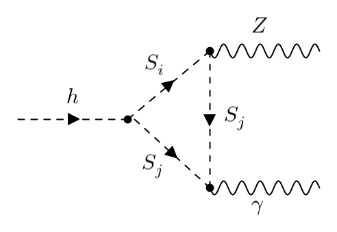
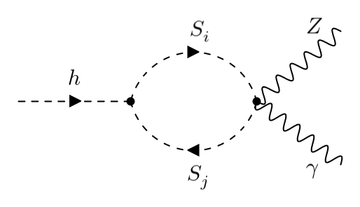
Figure 1: Representative Feynman diagrams that give additional contributions to $\mu_{Z\gamma}$ exclusively.

The strengths of the couplings required for accommodating nonstandard values $\mu_{Z\gamma}$ have been presented in Fig. 2. As can be observed from the figure, the quantity $g_{zs_{1}s_{2}}\lambda_{hs_{1}s_{2}}/m_{C}^{2}$ can be almost pinned down uniquely as a function of $\mu_{Z\gamma}$, $\frac{f(\mu_{Z\gamma})}{M_{W}^{2}}$, in the limit $m_{C1}=m_{C2}=m_{C}$ where $m_{Ci}$ denotes the mass of the $i$-th charged scalar. With this spirit we may approximately write

$$\frac{\lambda_{hs_{1}s_{2}}g_{zs_{1}s_{2}}}{m_{C}^{2}}\approx\frac{f(\mu_{Z\gamma})}{M_{W}^{2}}\,,$$ (3)

with the understanding that $f(\mu_{Z\gamma})=0$ for $\mu_{Z\gamma}=1$, as can be confirmed using Fig. 2. For a particular value of $\mu_{Z\gamma}$, the thickness of the black plot arises because $m_{C}$ is scanned from relatively low values, within the range 100 GeV $<m_{C}<$ 1 TeV. The thickness of the plot, for practical purposes, becomes negligible once we go beyond $m_{C}\gtrsim 250$ GeV as can be seen from the thin red overlaid region and in this case the equality in Eq. (3) becomes more robust.

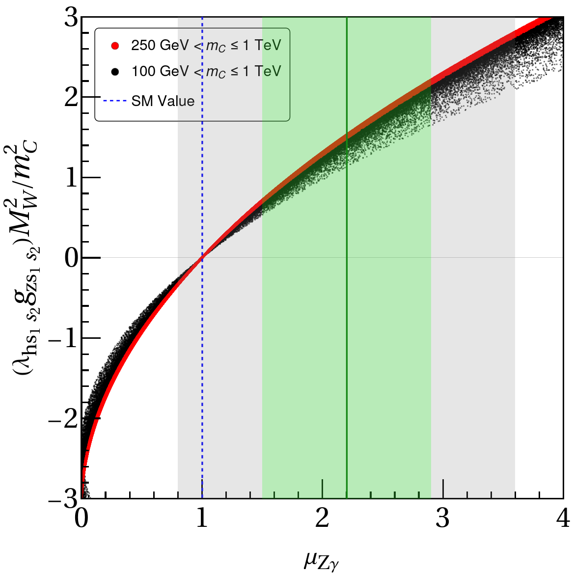
Figure 2: Required values of $f(\mu_{Z\gamma})$ (defined in Eq. (3)) as a function of $\mu_{Z\gamma}$. The common charged scalar mass ($m_{C1}=m_{C2}=m_{C}$) has been scanned within the range [100 GeV, 1 TeV] for the black region and within [250 GeV, 1 TeV] for the thin red region. The dark-green solid vertical line marks the currently measured central value of $\mu_{Z\gamma}$ and the light-green and gray vertical bands around it correspond to the $1\sigma$ and $2\sigma$ ranges respectively. The dashed blue vertical line denotes the SM value of $\mu_{Z\gamma}$.

Now that the essential strategy to accommodate a nonstandard $\mu_{Z\gamma}$ has been laid out, it might be reasonable to ask whether the couplings of Eq. (2) have any additional observable consequences which can potentially falsify such a scenario. A related study will be to investigate whether the couplings of Eq. (2) can arise from a more complete gauge theoretical framework. It is well-known that the off-diagonal charged scalar couplings can emerge whenever the physical charged scalars are derived from an admixture of two different $SU(2)_{L}\times U(1)_{Y}$ multiplets. The Zee-type[14] scalar potential constitutes a good example of such a scenario. For the Zee-type set-up, dominant off-diagonal couplings (with the $Z$-boson) overpowering the diagonal couplings can be achieved when the two charged scalars mix maximally[17].

However, instead of channeling our efforts to construct a specific model, we can follow a bottom-up method by exploring the high-energy unitarity behaviors of the tree-level scattering amplitudes[18] involving the couplings of Eq. (2). Such an analysis is known to reveal the compatibility of the set of couplings in Eq. (2) with a UV-complete gauge theory[21, 22]. If the interactions in Eq. (2) necessitate additional dynamics accompanying them, the scattering amplitudes are expected to possess undesirable energy growths which will lead to violation of tree-unitarity[23] at high energies. The energy scale at which unitarity is violated, can be interpreted as the maximum energy scale before which the effects of new physics must set in to restore unitarity. Such an exercise provides an alternative strategy to discover the need for additional effects that should be accompanied by an enhanced $\mu_{Z\gamma}$.

To demonstrate this explicitly we first calculate the amplitude for the process $Z_{L}Z_{L}\to S_{1}^{+}S_{1}^{-}$ where the subscript ‘$L$’ represents longitudinal polarization. In the high-energy limit, $E_{CM}\gg M$, meaning the CM energy is much larger than all the masses in our current theory, we obtain

$$-{\cal M}_{Z_{L}Z_{L}\to S_{1}^{+}S_{1}^{-}}\approx\frac{g_{zs_{1}s_{2}}^{2}}{M_{Z}^{2}}E_{\rm CM}^{2}-2g_{zs_{1}s_{2}}^{2}+{\cal O}\left(\frac{M^{2}}{E_{CM}^{2}}\right)\,,$$ (4)

where we have assumed $m_{C1}=m_{C2}\equiv m_{C}$. As it is evident, the first term in the above relation will definitely violate unitarity at high energies. This puts an upper limit on the CM-energy as follows:

$$\frac{g_{zs_{1}s_{2}}^{2}}{M_{Z}^{2}}E_{\rm CM}^{2}<16\pi\,.$$ (5)

Since all the new physics needs to intervene before unitarity violation

$$\frac{g_{zs_{1}s_{2}}^{2}}{M_{Z}^{2}}\Lambda_{NP}^{2}<16\pi\,.$$ (6)

We can ponder over what kind of new couplings would be required to fix this. But instead of that, we would rather choose to stay agnostic about the possible UV completions and make an effort to correlate the unitarity violation scale with the value of $\mu_{Z\gamma}$.

To achieve this, we also consider the process $Z_{L}Z_{L}\to S_{1}^{+}S_{2}^{-}$. In the high energy limit, the amplitude is found to be

$${\cal M}_{Z_{L}Z_{L}\to S_{1}^{+}S_{2}^{-}}\approx-\frac{g}{2}\lambda_{hs_{1}s_{2}}+{\cal O}\left(\frac{M^{2}}{E_{\rm CM}^{2}}\right)\,,$$ (7)

where $g$ is the $SU(2)_{L}$ gauge coupling. This puts an upper limit on $\lambda_{hs_{1}s_{2}}$ as follows

$$\left|\frac{g}{2}\lambda_{hs_{1}s_{2}}\right|<16\pi\,.$$ (8)

Eqs. (8) and (6) can be combined to write

$$\left|\lambda_{hs_{1}s_{2}}g_{zs_{1}s_{2}}\right|\Lambda_{NP}<M_{\rm max}\,,$$ (9a)

$${\rm with,} M_{\rm max}=\sqrt{(16\pi)^{3}}\frac{2M_{Z}}{g}\,.$$ (9b)

This can be used to cast a definite upper bound on $\Lambda_{NP}$ provided the value of the product $\lambda_{hs_{1}s_{2}}g_{zs_{1}s_{2}}$ can be estimated from other considerations. This is where the experimental determination of $\mu_{Z\gamma}$ becomes relevant. A nonstandard value of $\mu_{Z\gamma}$ exclusively, will necessitate such couplings whose strength can be estimated using Eq. (3). Keeping in mind the fact that the charged scalars are also parts of NP beyond the SM, Eq. (3) may be reshuffled to write

$$\lambda_{hs_{1}s_{2}}g_{zs_{1}s_{2}}=\frac{f(\mu_{Z\gamma})\Lambda_{\rm NP}^{2}}{M_{W}^{2}}\,.$$ (10)

Plugging this into Eq. (9) we may infer

$$\Lambda_{\rm NP}<\sqrt[3]{\frac{M_{\rm max}M_{W}^{2}}{\left|f(\mu_{Z\gamma})\right|}}\,.$$ (11)

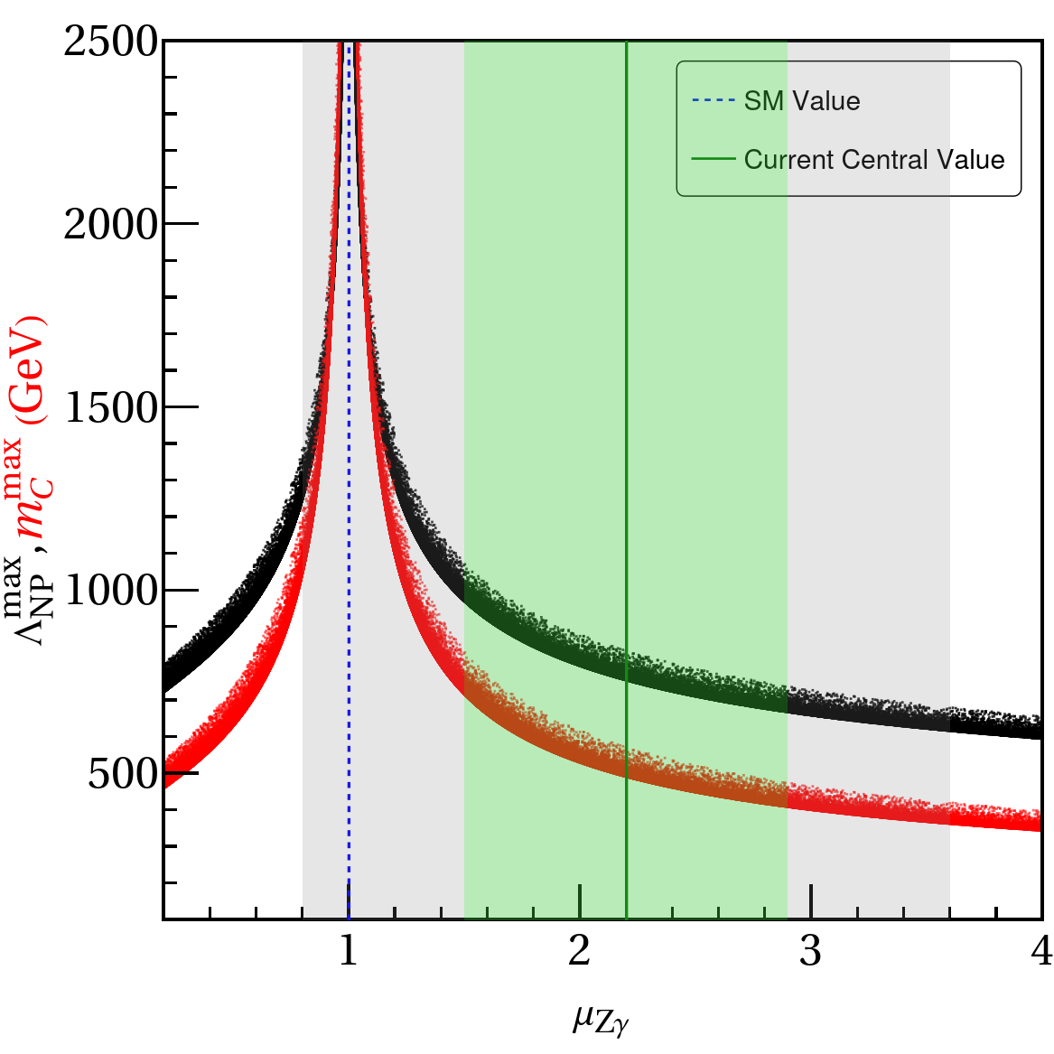
Figure 3: The upper limits in Eqs. (11) and (14) plotted against $\mu_{Z\gamma}$ as black and red regions respectively. The dark-green solid vertical line marks the currently measured central value of $\mu_{Z\gamma}$ and the light-green and gray vertical bands around it correspond to the $1\sigma$ and $2\sigma$ ranges respectively. The dashed blue vertical line denotes the SM value of $\mu_{Z\gamma}$.

It should be noted that, as $f(\mu_{Z\gamma}=1)=0$, the upper limit on $\Lambda_{\rm NP}$ can be infinitely large for $\mu_{Z\gamma}=1$, implying that the new physics effects can be safely decoupled in the SM-limit as expected. However a more intriguing thing to note will be the fact that any deviation of $\mu_{Z\gamma}$ from the SM value will mandate the intervention of new physics. To quantify the required proximity of the new physics scale, we plot the right hand side of Eq. (11) as the black region in Fig. 3 where the value of the function $f(\mu_{Z\gamma})$ is mapped from Fig. 2. From Fig. 3 we can see that new physics effects in the sub-TeV regime will be imminent even when $\mu_{Z\gamma}$ deviates from unity by only $20\%$. In fact, the current central value of $\mu_{Z\gamma}=2.2$ (marked by the dark-green vertical solid line) decrees $\Lambda_{\rm NP}$ to be below 500 GeV which should be well within the reach of the LHC.

In passing, we note that a more direct upper bound on the charged scalar masses can be placed by considering the scattering process $Z_{L}S^{+}_{1}\to hS_{1}^{+}$. In the high-energy limit the tree-level amplitude can be written as

$${\cal M}_{Z_{L}S^{+}_{1}\to hS_{1}^{+}} \approx -g_{zs_{1}s_{2}}\lambda_{hs_{1}s_{2}}\frac{M_{W}}{M_{Z}}+{\cal O}\left(\frac{M^{2}}{E_{\rm CM}^{2}}\right)\,.$$ (12)

Therefore the unitarity constraint should imply

$$\left|g_{zs_{1}s_{2}}\lambda_{hs_{1}s_{2}}\right|\frac{M_{W}}{M_{Z}}<16\pi\,.$$ (13)

Again using Eq. (6) we can translate the above inequality into an upper limit on the common charged scalar mass as follows:

$$m_{C}<\sqrt{16\pi\frac{M_{Z}M_{W}}{\left|f(\mu_{Z\gamma})\right|}}\,.$$ (14)

This upper limit has also been plotted in Fig. (3) as the scattered region in red which has a very similar interpretation to the black region discussed previously.

To summarize, recent experimental data on $\mu_{Z\gamma}$ instigates us to contemplate the possibility of having all the Higgs signal strengths in excellent agreement with the corresponding SM expectations, except $\mu_{Z\gamma}$ which deviates substantially from its SM value. Our current article can be considered as a theoretical preparation for such an eventuality in a bottom-up manner. We provided a general template for the new physics interactions which will exclusively affect $h\to Z\gamma$. We particularized our strategy with new charged scalars endowed with dominant off-diagonal couplings with the Higgs and the $Z$ bosons, as exemplified through Eq. (2). However, as we have explicitly shown, such interactions will compromise the unitarity of the theory. Consequently, we are able to place an upper bound on the common charged scalar mass, which can be as low as 500 GeV for the current central value of $\mu_{Z\gamma}$. This means that, if the current non-standard value of $\mu_{Z\gamma}$ becomes statistically significant as more data accumulates, discovery of new physics effects at the LHC should be just around the corner. The charged scalars, owing to their couplings with the photon, can be pair-produced by the Drell-Yan mechanism [24, 25]. The subsequent decay modes of these charged scalars will, of course, depend on the finer details of the BSM scenario from which they arise. Even if the charged scalars are stable, they can be probed in the ongoing searches for long-lived charged particles [26, 27]. This anticipatory experimental scenario may be compared with the status of the LHC in the pre-Higgs-discovery era, as a win-win machine in the sense that the LHC should either observe the Higgs-boson or something equivalent, or violation of unitarity at high energies. In a similar spirit, LHC can again act as a win-win experiment for BSM searches if $\mu_{Z\gamma}$ eventually settles towards a nonstandard value. That would definitely be an exciting future to look forward to.

Appendix A Explicit calculations of the scattering amplitudes

In this appendix, we show the explicit calculations of the scattering amplitudes discussed in the main text. First we consider the process

$$\centering\Huge Z_{L}(p_{1})+Z_{L}(p_{2})\to S_{1}^{+}(k_{1})+S_{1}^{-}(k_{2})\,.\@add@centering$$ (A.1)

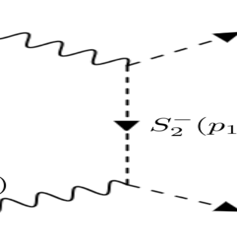
Figure 4: Feynman diagrams for $Z_{L}Z_{L}\to S_{1}^{+}S_{1}^{-}$.

The vertex factor for the interaction $Z_{\mu}S_{1}^{+}(p)S_{2}^{-}(p^{\prime})$ is written as $ig_{zs_{1}s_{2}}(p-p^{\prime})_{\mu}$ where, $p$ and $p^{\prime}$ are the momenta of the incoming charged scalars. Considering the momentum assignment of the initial and final states particles as in Eq. (A.1), we can write

$$p_{1}+p_{2}=k_{1}+k_{2}\,.$$ (A.2)

Now, the Feynman amplitude for the $t$-channel diagram is given by,

$$i{\cal M}_{t} = (ig_{zs_{1}s_{2}})^{2}\left[-(p_{1}-k_{1})+k_{1}\right]_{\mu}\frac{i}{t-m_{C_{2}}^{2}}\left[-k_{2}-\left(p_{1}-k_{1}\right)\right]_{\nu}\epsilon^{\mu}(p_{1})\epsilon^{\nu}(p_{2})\,,$$ (A.3)

$$= \frac{ig_{zs_{1}s_{2}}^{2}}{t-m_{C_{2}}^{2}}\left(p_{1}-2k_{1}\right)_{\mu}\epsilon^{\mu}(p_{1})\left(p_{2}-2k_{2}\right)_{\nu}\epsilon^{\nu}(p_{2})\,,$$

where we used Eq. (A.2) in the last step. In a similar manner, we write down the matrix element for the $u$-channel diagram as,

$$i{\cal M}_{u} = (ig_{zs_{1}s_{2}})^{2}\left[-k_{2}-\left(k_{2}-p_{1}\right)\right]_{\mu}\frac{i}{u-m_{C_{2}}^{2}}\left[k_{1}-\left(k_{2}-p_{1}\right)\right]_{\nu}\epsilon^{\mu}(p_{1})\epsilon^{\nu}(p_{2})\,,$$ (A.4)

$$= \frac{ig_{zs_{1}s_{2}}^{2}}{u-m_{C_{2}}^{2}}\left(p_{1}-2k_{2}\right)_{\mu}\epsilon^{\mu}(p_{1})\left(p_{2}-2k_{1}\right)_{\nu}\epsilon^{\nu}(p_{2})\,.$$

Next, we express the longitudinal polarization vector for the $Z$-boson as $\epsilon_{L}^{\mu}(p)\equiv{\epsilon^{\mu}(p)}/{M_{Z}}$ with the understanding that $\epsilon^{\mu}(p)\epsilon_{\mu}(p)=-M_{Z}^{2}$ and $p_{\mu}\epsilon^{\mu}(p)=0$. The kinematics for the process in the CM frame has been schematically depicted in fig. 5. Following this, we may write

$$k_{1}\cdot\epsilon_{L}(p_{1})=\frac{E}{M_{Z}}(p-k\cos\theta)=k_{2}\cdot\epsilon_{L}(p_{2})\,;$$ (A.5a)

$$k_{2}\cdot\epsilon_{L}(p_{1})=\frac{E}{M_{Z}}(p+k\cos\theta)=k_{1}\cdot\epsilon_{L}(p_{2})\,.$$ (A.5b)

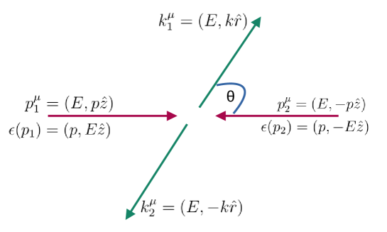
Figure 5: Kinematics in the CM frame for the process in Eq. (A.1).

Using the relations given in Eq. (A.5), we now rewrite the matrix elements as,

$${\cal M}_{t} = 4g_{zs_{1}s_{2}}^{2}\frac{E^{2}}{M_{Z}^{2}}\frac{(p-k\cos\theta)^{2}}{t-m_{C_{2}}^{2}}\,,$$ (A.6a)

$${\cal M}_{u} = 4g_{zs_{1}s_{2}}^{2}\frac{E^{2}}{M_{Z}^{2}}\frac{(p+k\cos\theta)^{2}}{u-m_{C_{2}}^{2}}\,.$$ (A.6b)

Now, using $t=(p_{1}-k_{1})^{2}$ and $u=(p_{2}-k_{1})^{2}$ in combination with Eq. (A.2), we can show that

$$\left(p-k\cos\theta\right) = \frac{\Delta m^{2}-t}{2p}\,,$$ (A.7a)

$$\left(p+k\cos\theta\right) = \frac{\Delta m^{2}-u}{2p}\,,$$ (A.7b)

where, we have defined $\Delta m^{2}=m_{C_{1}}^{2}-M_{Z}^{2}$. Thus, substituting Eq. (A.7) into Eqs. (A.6), we find,

$${\cal M}_{t} = \frac{g_{zs_{1}s_{2}}^{2}E^{2}}{p^{2}M_{Z}^{2}}\left(\Delta m^{2}-t\right)^{2}\frac{1}{t}\left(1-\frac{m_{C_{2}}^{2}}{t}\right)^{-1}\,,$$ (A.8a)

$$\Rightarrow{\cal M}_{t} \simeq \frac{g_{zs_{1}s_{2}}^{2}E^{2}}{p^{2}M_{Z}^{2}}\left(t-2\Delta m^{2}+m_{C_{2}}^{2}\right)\,,$$ (A.8b)

$${\rm and,~{}similarly}\quad{\cal M}_{u} \simeq \frac{g_{zs_{1}s_{2}}^{2}E^{2}}{p^{2}M_{Z}^{2}}\left(u-2\Delta m^{2}+m_{C_{2}}^{2}\right)\,,$$ (A.8c)

where, we have neglected the terms ${\cal O}(M^{2}/E^{2})$ in the high-energy limit. Furthermore, using the identity

$$\frac{E^{2}}{p^{2}}=E^{2}(E^{2}-M_{Z}^{2})^{-1}\simeq\left(1+\frac{M_{Z}^{2}}{E^{2}}\right)\,,$$ (A.9)

we reduce the above amplitudes into,

$${\cal M}_{t} = \frac{g_{zs_{1}s_{2}}^{2}}{M_{Z}^{2}}t+g_{zs_{1}s_{2}}^{2}\left[\frac{t}{E^{2}}-\frac{\Lambda^{2}}{M_{Z}^{2}}\right]+{\cal O}\left(\frac{M^{2}}{E^{2}}\right)\,,$$ (A.10a)

$${\rm and,}\quad{\cal M}_{u} = \frac{g_{zs_{1}s_{2}}^{2}}{M_{Z}^{2}}u+g_{zs_{1}s_{2}}^{2}\left[\frac{u}{E^{2}}-\frac{\Lambda^{2}}{M_{Z}^{2}}\right]+{\cal O}\left(\frac{M^{2}}{E^{2}}\right)\,,$$ (A.10b)

where we defined $\Lambda^{2}=(2\Delta m^{2}-m_{C_{2}}^{2})$. Thus the total amplitude will be given by,

$${\cal M}_{Z_{L}Z_{L}\to S_{1}^{+}S_{1}^{-}}=({\cal M}_{t}+{\cal M}_{u})=\frac{g_{zs_{1}s_{2}}^{2}}{M_{Z}^{2}}(t+u)+g_{zs_{1}s_{2}}^{2}\left[\frac{(t+u)}{E^{2}}-\frac{2\Lambda^{2}}{M_{Z}^{2}}\right]+{\cal O}\left(\frac{M^{2}}{E^{2}}\right)\,.$$ (A.11)

Substituting $t+u=2(M_{Z}^{2}+m_{C_{1}}^{2})-4E^{2}$ we obtain,

$$-{\cal M}_{Z_{L}Z_{L}\to S_{1}^{+}S_{1}^{-}}=\frac{4g_{zs_{1}s_{2}}^{2}}{M_{Z}^{2}}E^{2}-\frac{g_{zs_{1}s_{2}}^{2}}{M_{Z}^{2}}\left[2(M_{Z}^{2}+m_{C_{1}}^{2})-2\Lambda^{2}-4M_{Z}^{2}\right]+{\cal O}\left(\frac{M^{2}}{E^{2}}\right)\,,$$ (A.12a)

$$\Rightarrow -{\cal M}_{Z_{L}Z_{L}\to S_{1}^{+}S_{1}^{-}}\approx\frac{4g_{zs_{1}s_{2}}^{2}}{M_{Z}^{2}}E^{2}-\frac{2g_{zs_{1}s_{2}}^{2}}{M_{Z}^{2}}\left[M_{Z}^{2}+\left(m_{C_{1}}^{2}-m_{C_{2}}^{2}\right)\right]\,,$$ (A.12b)

$$\Rightarrow -{\cal M}_{Z_{L}Z_{L}\to S_{1}^{+}S_{1}^{-}}\approx\frac{g_{zs_{1}s_{2}}^{2}}{M_{Z}^{2}}E_{\rm CM}^{2}-2g_{zs_{1}s_{2}}^{2}+\frac{2g_{zs_{1}s_{2}}^{2}}{M_{Z}^{2}}\left(m_{C_{1}}^{2}-m_{C_{2}}^{2}\right)\,,$$ (A.12c)

where $E_{\rm CM}=2E$.

Next we consider the process

$$\centering\Huge Z_{L}(p_{1})+Z_{L}(p_{2})\to S_{1}^{+}(k_{1})+S_{2}^{-}(k_{2})\,.\@add@centering$$ (A.13)

Since we are assuming the presence of off-diagonal couplings only, with the Higgs and the $Z$-boson, the above process can only proceed via the $s$-channel Higgs exchange. The corresponding amplitude will be given by

$$i{\cal M}_{Z_{L}Z_{L}\to S_{1}^{+}S_{2}^{-}} = \left(\frac{igM_{Z}}{c_{w}}\right)\frac{i}{s-m_{h}^{2}}\left(i\lambda_{hs_{1}s_{2}}M_{W}\right)\epsilon_{L}^{\mu}(p_{1})\epsilon_{L\mu}(p_{2})\,,$$ (A.14a)

$$\Rightarrow{\cal M}_{Z_{L}Z_{L}\to S_{1}^{+}S_{2}^{-}} = \left(-gM_{Z}^{2}\lambda_{hs_{1}s_{2}}\right)\frac{1}{s-m_{h}^{2}}\frac{\left(p^{2}+E^{2}\right)}{M_{Z}^{2}}\,,$$ (A.14b)

where, $g$ is the $SU(2)_{L}$ gauge coupling, $c_{w}$ represents the cosine of the weak mixing angle and we used $p_{1}^{\mu}=(E,p\hat{z})$ and $p_{2}^{\mu}=(E,-p\hat{z})$ in the CM frame. Furthermore, using $p^{2}+E^{2}=s/2-M_{Z}^{2}$ we get,

$${\cal M}_{Z_{L}Z_{L}\to S_{1}^{+}S_{2}^{-}} \approx -\frac{1}{2}g\lambda_{hs_{1}s_{2}}+{\cal O}\left(\frac{M^{2}}{E^{2}}\right)\,.$$ (A.15)

Finally, we consider the process

$$\centering\Huge Z_{L}(p_{1})+S^{+}_{1}(p_{2})\to h(k_{1})+S_{1}^{+}(k_{2})\,.\@add@centering$$ (A.16)

The Feynman diagram along with the kinematics in the CM frame have been depicted in Fig. 6.

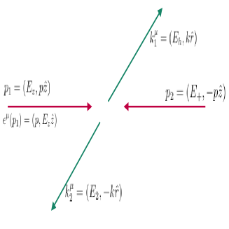
Figure 6: Feynman diagram for the process appearing in Eq. (A.16) and the corresponding kinematics in the CM frame.

The amplitude for the process may be written as,

$$i{\cal M}_{Z_{L}S_{1}^{+}\to hS_{1}^{+}}=ig_{zs_{1}s_{2}}\left\{p_{2}+(p_{1}+p_{2})\right\}_{\mu}\frac{i}{s-m_{C_{2}}^{2}}(i\lambda_{hs_{1}s_{2}}M_{W})\epsilon_{L}^{\mu}(p_{1})\,,$$ (A.17a)

$$\Rightarrow {\cal M}_{Z_{L}S_{1}^{+}\to hS_{1}^{+}}=-g_{zs_{1}s_{2}}\lambda_{hs_{1}s_{2}}\frac{M_{W}}{M_{Z}}\frac{1}{s-m_{C_{2}}^{2}}\left(2p_{2}\cdot\epsilon(p_{1})\right)\,.$$ (A.17b)

Now, following the kinematics in Fig. 6 we have the following relations,

$$p_{2}\cdot\epsilon(p_{1})=(E_{+}p+E_{z}p)=p(E_{+}+E_{z})\equiv p\sqrt{s}\,,$$ (A.18a)

$${\rm and,} p^{2}=E_{z}^{2}-M_{Z}^{2}=E_{+}^{2}-m_{C_{1}}^{2}\,,$$ (A.18b)

$$\Rightarrow M_{Z}^{2}-m_{C_{1}}^{2}=E_{z}^{2}-E_{+}^{2}\,,$$ (A.18c)

$$\Rightarrow (E_{z}-E_{+})=\frac{M_{Z}^{2}-m_{C_{1}}^{2}}{\sqrt{s}}\,.$$ (A.18d)

Alternatively, one can also write,

$$2p^{2} = E_{z}^{2}+E_{+}^{2}-(M_{Z}^{2}+m_{C_{1}}^{2})\,,$$ (A.19a)

$$= \frac{1}{2}\left[(E_{+}+E_{z})^{2}+(E_{+}-E_{z})^{2}\right]-(M_{Z}^{2}+m_{C_{1}}^{2})\,,$$

$$= \frac{1}{2}\left[s+\frac{(M_{Z}^{2}-m_{C_{1}}^{2})^{2}}{s}-2(M_{Z}^{2}+m_{C_{1}}^{2})\right]\,,$$

$$\Rightarrow p^{2} = \frac{1}{4}\left[s+\frac{(M_{Z}^{2}-m_{C_{1}}^{2})^{2}}{s}-2(M_{Z}^{2}+m_{C_{1}}^{2})\right]\,,$$ (A.19b)

$$\Rightarrow p = \frac{\sqrt{s}}{2}\left[1-2\frac{(M_{Z}^{2}+m_{C_{1}}^{2})}{s}+\frac{(M_{Z}^{2}-m_{C_{1}}^{2})^{2}}{s^{2}}\right]^{\frac{1}{2}}\,,$$ (A.19c)

$$p \approx \frac{\sqrt{s}}{2}\left[1-\frac{(M_{Z}^{2}+m_{C_{1}}^{2})}{s}+{\cal O}\left(\frac{M^{4}}{s^{2}}\right)\right]\,.$$ (A.19d)

Thus, one may write

$$p_{2}\cdot\epsilon(p_{1}) = \frac{s}{2}\left[1-\frac{(M_{Z}^{2}+m_{C_{1}}^{2})}{s}+{\cal O}\left(\frac{M^{4}}{s^{2}}\right)\right]\,.$$ (A.20)

Using this in Eq. (A.17b), the final expression for the amplitude, in the high-energy limit, can be written as

$${\cal M}_{Z_{L}S_{1}^{+}\to hS_{1}^{+}}\approx-g_{zs_{1}s_{2}}\lambda_{hs_{1}s_{2}}\frac{M_{W}}{M_{Z}}+{\cal O}\left(\frac{M^{2}}{s}\right)\,.$$ (A.21)

References

• [1] ATLAS Collaboration, G. Aad et al., Observation of a new particle in the search for the Standard Model Higgs boson with the ATLAS detector at the LHC, Phys. Lett. B 716 (2012) 1–29, [arXiv:1207.7214].
• [2] CMS Collaboration, S. Chatrchyan et al., Observation of a New Boson at a Mass of 125 GeV with the CMS Experiment at the LHC, Phys. Lett. B 716 (2012) 30–61, [arXiv:1207.7235].
• [3] G. Bhattacharyya and D. Das, Nondecoupling of charged scalars in Higgs decay to two photons and symmetries of the scalar potential, Phys. Rev. D 91 (2015) 015005, [arXiv:1408.6133].
• [4] G. D. Kribs, T. Plehn, M. Spannowsky, and T. M. P. Tait, Four generations and Higgs physics, Phys. Rev. D 76 (2007) 075016, [arXiv:0706.3718].
• [5] O. Eberhardt, G. Herbert, H. Lacker, A. Lenz, A. Menzel, U. Nierste, and M. Wiebusch, Impact of a Higgs boson at a mass of 126 GeV on the standard model with three and four fermion generations, Phys. Rev. Lett. 109 (2012) 241802, [arXiv:1209.1101].
• [6] A. Djouadi and A. Lenz, Sealing the fate of a fourth generation of fermions, Phys. Lett. B 715 (2012) 310–314, [arXiv:1204.1252].
• [7] T. Bandyopadhyay, D. Das, R. Pasechnik, and J. Rathsman, Complementary bound on the $W^{\prime}$ mass from Higgs boson to diphoton decays, Phys. Rev. D 99 (2019), no. 11 115021, [arXiv:1902.03834].
• [8] ATLAS Collaboration, G. Aad et al., A search for the $Z\gamma$ decay mode of the Higgs boson in $pp$ collisions at $\sqrt{s}$ = 13 TeV with the ATLAS detector, Phys. Lett. B 809 (2020) 135754, [arXiv:2005.05382].
• [9] CMS, ATLAS Collaboration, G. Aad et al., Evidence for the Higgs boson decay to a $Z$ boson and a photon at the LHC, arXiv:2309.03501.
• [10] CMS Collaboration, A. Tumasyan et al., Search for Higgs boson decays to a Z boson and a photon in proton-proton collisions at $\sqrt{s}$ = 13 TeV, JHEP 05 (2023) 233, [arXiv:2204.12945].
• [11] J. F. Gunion, H. E. Haber, G. L. Kane, and S. Dawson, The Higgs Hunter’s Guide, vol. 80. 2000.
• [12] A. Djouadi, The Anatomy of electro-weak symmetry breaking. I: The Higgs boson in the standard model, Phys. Rept. 457 (2008) 1–216, [hep-ph/0503172].
• [13] L. T. Hue, A. B. Arbuzov, T. T. Hong, T. P. Nguyen, D. T. Si, and H. N. Long, General one-loop formulas for decay $h\rightarrow Z\gamma$, Eur. Phys. J. C 78 (2018), no. 11 885, [arXiv:1712.05234].
• [14] A. Zee, A Theory of Lepton Number Violation, Neutrino Majorana Mass, and Oscillation, Phys. Lett. B 93 (1980) 389. [Erratum: Phys.Lett.B 95, 461 (1980)].
• [15] D. Barducci, L. Di Luzio, M. Nardecchia, and C. Toni, Closing in on new chiral leptons at the LHC, arXiv:2311.10130.
• [16] T. T. Hong, V. K. Le, L. T. T. Phuong, N. . C. Hoi, N. T. K. Ngan, and N. H. T. Nha, Decays of standard model like higgs boson $h\rightarrow\gamma\gamma,z\gamma$ in a minimal left-right symmetric model, arXiv:2312.11045.
• [17] R. R. Florentino, J. C. Romão, and J. P. Silva, Off diagonal charged scalar couplings with the Z boson: Zee-type models as an example, Eur. Phys. J. C 81 (2021), no. 12 1148, [arXiv:2106.08332].
• [18] J. F. Gunion, H. E. Haber, and J. Wudka, Sum rules for Higgs bosons, Phys. Rev. D 43 (1991) 904–912.
• [19] F. Abu-Ajamieh, The scale of new physics from the Higgs couplings to $\gamma$ $\gamma$ and $\gamma$Z, JHEP 06 (2022) 091, [arXiv:2112.13529].
• [20] G. Bhattacharyya, D. Das, and P. B. Pal, Modified Higgs couplings and unitarity violation, Phys. Rev. D 87 (2013) 011702, [arXiv:1212.4651].
• [21] C. H. Llewellyn Smith, High-Energy Behavior and Gauge Symmetry, Phys. Lett. B 46 (1973) 233–236.
• [22] J. M. Cornwall, D. N. Levin, and G. Tiktopoulos, Derivation of Gauge Invariance from High-Energy Unitarity Bounds on the s Matrix, Phys. Rev. D 10 (1974) 1145. [Erratum: Phys.Rev.D 11, 972 (1975)].
• [23] B. W. Lee, C. Quigg, and H. B. Thacker, Weak Interactions at Very High-Energies: The Role of the Higgs Boson Mass, Phys. Rev. D 16 (1977) 1519.
• [24] A. Alves and T. Plehn, Charged Higgs boson pairs at the CERN LHC, Phys. Rev. D 71 (2005) 115014, [hep-ph/0503135].
• [25] A. Banerjee et al., Phenomenological aspects of composite Higgs scenarios: exotic scalars and vector-like quarks, arXiv:2203.07270.
• [26] J. J. Heinrich, Search for charged stable massive particles with the ATLAS detector, Ph. D. Thesis (2018) CERN–THESIS–2018–165.
• [27] ATLAS Collaboration, M. Aaboud et al., Search for heavy charged long-lived particles in the ATLAS detector in 36.1 fb-1 of proton-proton collision data at $\sqrt{s}=13$ TeV, Phys. Rev. D 99 (2019), no. 9 092007, [arXiv:1902.01636].