Energy norm error estimates and convergence analysis for a stabilized
Maxwell’s equations in conductive media
E. Lindström
Eric Lindström, Email: erilinds@chalmers.seL. Beilina
Larisa Beilina, Email: larisa@chalmers.se
Department of Mathematical Sciences, Chalmers University of Technology and University of Gothenburg, SE-412 96 Gothenburg Sweden
Abstract
The aim of this article is to investigate the well-posedness,
stability and convergence of solutions to the time-dependent
Maxwell’s equations for electric field in conductive media in
continuous and discrete settings. The situation we consider would
represent a physical problem where a subdomain is emerged in a
homogeneous medium, characterized by constant dielectric
permittivity and conductivity functions. It is well known that in
these homogeneous regions the solution to the Maxwell’s equations
also solves the wave equation which makes calculations very
efficient. In this way our problem can be considered as a coupling
problem for which we derive stability and convergence analysis. A number
of numerical examples validate theoretical convergence rates of the
proposed stabilized explicit finite element scheme.
Keywords: Maxwell’s equations, finite element method, stability, a priori error analysis, energy error estimate, convergence analysis
In this paper we consider the time-dependent Maxwell’s equations in a
bounded, simply connected spatial domain . This domain is
divided into two subdomains, one outer were the dielectric
permittivity and conductivity are constant functions, and one inner
one were they are allowed to vary but are still bounded functions.
One important (and of special interest for the authors) consequence of
the results developed in this paper are applications of Maxwell’s
equations to solutions of Coefficient Inverse Problems
(CIPs). In [40, 41] one can read about inverse
problems applied to imaging of buried objects, and in
[9, 10, 14] inverse problems are used for medical imaging. In
the latter case the problem is to reconstruct the dielectric
permittivity and conductivity functions of an anatomically realistic
phantom of a breast tissue.
The dielectric properties of different tissue types in a breast are
experimentally measured and known [26], but their
distribution inside every particular breast tissue is unknown. Such
a scenario is one case where the domain decomposition can be an useful
tool for solution of electromagnetic CIPs when the goal is
determination of dielectric properties of the object from boundary measurements of
the scattered electric field.
Under certain
circumstances, it is known that the solution to the Maxwell’s
equations also solves the wave equation, which is more studied and
understood, see [5, 6, 8, 9, 11].
In [11], a finite element analysis shows stability
and consistency of the stabilized finite element method for the
solution of Maxwell’s equations in non-conductive media, and
in [5] authors investigated a stabilized domain decomposition
finite element method for the time
harmonic Maxwell’s equations. Stability and convergence analysis of a Domain Decomposition FE/FD
method for time-dependent Maxwell’s equations was presented in [6].
In our knowledge, all previous cited
works consider non-conductive media, and the research concerning
time-dependent Maxwell’s equation for electric field in conductive media, when both dielectric
permittivity and conductivity are space-dependent functions, are
missing.
The stability and well-posedness of the wave equation are well
understood and studied [24, 32]. Certain model of wave equations
have also been used to model inverse problems, see
[12, 7, 25]. The progression to Maxwell’s equations is
arguably natural, since the system has wave-like properties. However,
some complications occur from the presence of the double curl
operator.
Another theoretical complication is that when one analyzes the
corresponding bilinear form induced by the variational form, one can
see that it is not coercive. This coercivity is often critical in
proofs concerning existence and uniqueness of solutions. The
additional novelty of the presented work is in how we deal with
coercivity of the bilinear form. Since the bilinear form with presence
of time-dependent terms is non-coercive, we split it and separate
terms with derivatives in time in order to derive the coercivity for
the remaining spatial part of the bilinear form using some minor
restrictions on the gradient of the permittivity function. We use
then coercivity of the spatial part of the bilinear form in the proof
of a priori error estimate. Derivation of coercivity of the entire scheme is a topic of an ongoing research.
To align the results with implementations of -methods, we
introduce a slightly altered, stabilized problem. Otherwise, these
methods can lead to spurious solutions (see
[4, 8, 16, 17, 27, 28, 29, 30, 36, 38])
and is well-known that theoretically, divergence free edge edge
elements are a better fit, see
[18, 22, 34, 35, 37]. To read more about various
numerical methods for Maxwell equations and more details about the
complications, see
[3, 4, 5, 15, 19, 20, 22, 23, 34, 36]
and references therein.
Naturally, since the theoretical results of this work have importance
for numerical implementations, we also present analysis of the
corresponding discrete problem to our original pmodel.
An outline of this paper is as follows.
In Section 2 we introduce the mathematical model and present the stabilized
problem
for the time-dependent Maxwell’s equations in conductive media.
In Section 3 we state the variational problem
for the stabilized model and
formulate the finite element scheme.
Section 4 is devoted to the energy norm error analysis
and section 5 presents derivation of a priori error estimates.
In Section 6 are performed
numerical convergence tests illustrating theoretical results of this paper.
Finally, in Section 7 we conclude the results of the paper.
2 The mathematical model
Let us consider
the initial value problem for the
electric field ,
, , for time-dependent
Maxwell’s equations in conductive media, under the
assumptions that the dimensionless relative magnetic permeability of
the medium is :
(1)
Here,
is the dimensionless relative dielectric permittivity,
is the
electric conductivity function; , and
are the permittivity and permeability of the free space,
respectively, and is the speed of
light in free space and is a given source function.
To solve the problem (1) numerically, we consider it in a
bounded simply connected space domain with
boundary and time domain .
In this work we will study the problem (1) in a special framework: we
decompose the space domain into two subdomains such that
and .
We assume that for some known constants chosen such that , the functions
satisfy following conditions:
(2)
We refer to [9] and references therein for justification and possible choice of these coefficients.
We observe that conditions (2) on and
together with the relation
(3)
and divergence free condition in ,
make equations in
(1) independent of each others in such that
in ,
we solve the system of uncoupled wave equations:
(4)
In [11], a finite element analysis shows stability
and consistency of the stabilized finite element method for the
solution of (1) with .
In [5] a stabilized linear, domain decomposition
finite element method for the time
harmonic Maxwell’s equations was studied.
In the current study
we show stability and convergence analysis of the finite element method for solution
of (1)
under the condition (2) on and .
Let .
Let us
introduce the following spaces of real valued functions
(5)
In this paper we study the following stabilized initial boundary value problem setting
: find
such that
(6)
Here, the divergence free condition is hidden in the first equation of system (6).
3 Finite Element Discretization
Throughout the paper
we denote the inner product in space
of
by , and the corresponding norm by .
Let us define the following scalar products used in the analysis:
(7)
Additionally, we define the -weighted norm
(8)
together with the -weighted scalar product:
(9)
To write finite element scheme to solve the model problem (6) in whole
,
we discretize
by partition of into elements , where
is a mesh function
defined as . Here, where
denotes the local diameter of the element .
We also denote by a partition of
the boundary into boundaries of the elements . Let be a uniform partition of the time interval into
equidistance subintervals with the time step
We also
assume a minimal angle condition on elements in [2, 33].
To formulate
the
finite element method
for the spatial semi-discrete problem (6)
in
we introduce the finite element space for every
component of the electric field defined by
where denote the set of piecewise-linear functions on .
We define to be the
usual interpolants of
, respectively,
in (6) onto .
Setting and
where the test function space is chosen as
We observe that boundary terms in (12) disappear because of definition of test space (10).
Thus, the bilinear form (12) for the case of test space (10) will be transformed to
(13)
Let us recall the explicit
fully discrete finite element scheme for solution of (11)
for
and
which was derived in [10]:
(14)
In the scheme
(14) we approximated and
by and , respectively, for .
Rearranging terms in (14) we get for
and
(15)
For the convergence of this scheme the following CFL condition derived in [11] for the case of should hold:
(16)
where is a mesh independent constant.
The CFL condition for
the case when both functions is topic of ongoing research.
4 Energy norm error estimate (stability estimate)
In this section first we give a proof of energy estimate,
for the vector of
the continuous model problem (6). Then we formulate
stability estimate for semi-discrete problem which is consequence of the energy
estimate for the continuous problem.
Theorem 4.1.
Assume that condition
(2) on the functions hold. Let be a bounded domain with the piecewise smooth
boundary . For any let and Suppose that
there exists a solution of
the model problem (6).
Then the vector is unique and there exists a constant
such that
the following energy estimate is true for all in
(6):
Through the proof we denote a generic constant of moderate size by . To prove our energy estimate we multiply (18) by and integrate over , and study it term by term. For the first term in (18) we have
(19)
where we used the chain rule, fundamental theorem of calculus and boundary conditions of (6).
Next we have that
(20)
where we use spatial integration by part, boundary conditions and that .
For the third term in (18) we integrate by parts spatially twice and get
(21)
Above we made use of (2) (note that since on a neighbourhood of , we have and ). We also made use of the fact that .
Before estimating the fourth term in (18) we first note that
and using that we get
If we then integrate these terms over we arrive at
One application of Grönwall’s inequality now gives us the result in (17).
∎
The next corollary follows from the stability estimate for the continuous
problem where all components of the electric field are replaced with their approximations , as well as all other continuous functions are replaced with their discrete analogs.
Corollary 4.1.
Assume that condition
(2) on the functions hold.
For any let and Suppose that
there exists a solution of
the problem (11) and the approximations of the initial data
and satisfy the regularity conditions
.
Then is unique and there exists a constant
such that
the following energy estimate is true for all in
(11):
(25)
5 A priori error estimates
In this section we present an a priori error estimate for
the error between the solution
of the
model problem (6) and solution of the
semi-discretized problem (11).
Let
(26)
where , . Here,
is an elliptic projection operator for , see details in [2, 21], such that
(27)
The first part of error, , can be estimated as follows.
Theorem 5.1.
Let bet the solution of the continuous problem (6).
Then
(28)
For
semi-discretized problem (11) these estimates
reduces to:
Taking in (31) , where is nodal interpolant of ,
and using
standard interpolation error estimates [21, 31, 13]
for
the fully discrete scheme in space and time
we get
(32)
where are interpolation constants.
For
semi-discretized problem (11) terms with disappear
and these estimates
reduces to (29).
∎
In the proof of a priori error estimate
we use the constant as a moderate constant which is adjusted throughout the proof, as well as well-posedness of the bilinear form . Let us briefly sketch the proof of well-posedness of .
We refer to [5] for the full details of this proof.
Since we can use the following estimate derived in [5]:
(42)
Using (42) and assumption (35) we obtain coercivity of
:
(43)
To prove continuity of , we
use Cauchy-Schwarz’ inequality and estimate (42)
to obtain :
(44)
Finally, we can verify continuity of :
(45)
∎
Theorem 5.3.
Let solves the continuous problem (6), and solves the semi-discretized problem (11). Assume that .
Further assume that the assumptions (2) and (35) on functions and hold, as well as , and . Then there exists a constant such that for all the following a priori error estimates hold:
(46)
Proof.
Since
is estimated via standard interpolation error estimates (28), we begin to estimate .
We first note that
By subtracting the first equation of (11) from the expression above, while letting we arrive at
(49)
Note that
by the properties of and Galerkin orthogonality.
Using this we observe that in (49) the term .
Thus, we can estimate a lower bound of the left-hand side of (49) as
(50)
where we have used that and .
We can also estimate an upper bound for the right-hand side of (49):
(51)
Collecting these two estimates, we have
(52)
Integrating over where and using conditions
(2) for functions noting that
we get
Summing up (28),
(60) and (61)
we get the desired error estimates (46),
and the proof is complete.
∎
6 Numerical examples
a)
b)
c)
d)
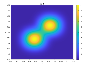
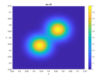
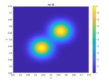
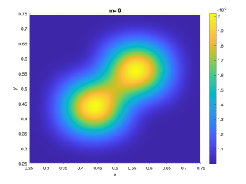
Figure 1: a) The function in the domain for different
values of in (64)
.
a)
b)
c)
d)
Figure 2: a) The function in the domain for different
values of in (64)
.
a)
b)
c)
d)
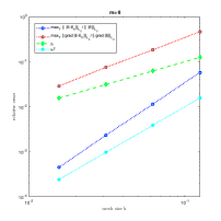
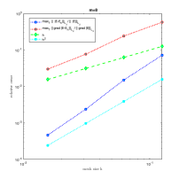
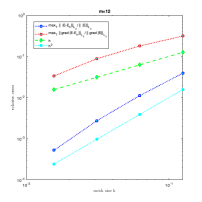
Figure 3: Relative errors for different in (64), (65)
.
In this section we perform computations which will confirm theoretical predictions given in Theorem 4.
All computations are performed in the software package WavES [42] using C++/PETSC [39].
The computational domain is chosen as with
such that .
To discretize the computational domain
we denote
by a partition of the domain into
triangles of sizes .
The explicit finite element scheme (15)
derived in [10] was used in computations.
We have chosen the time step such that the whole explicit scheme remains stable.
We have used following time-dependent model problem in computations:
(62)
The source data
is
computed by knowing the exact solution
In the model problem
(62)
the function is defined as
(64)
and the function as
(65)
Figures 1, 2 show the functions and , respectively,
for different in (64), (65) which were used in computations.
Relative errors
are computed at the time moment as
(66)
(67)
in - and
-norms,
respectively.
Here, is the exact solution
given by (63), and is the computed solution. We note also that
(68)
Figures 3 present convergence results of explicit finite element scheme
(15)
for the functions and defined by (64),
(65), respectively, for different values of .
Table 1, Table 2, Table 3 and Table 4 present
relative errors and convergence rates in the -norm and in the -norm for
mesh sizes ,
for different values of in (64),(65).
We note that chosen values of satisfy the regularity assumptions on the exact solution, see details in [11].
We used following expressions to compute convergence
rates and presented in these figures and tables:
(69)
where are computed relative norms
on the mesh with the mesh sizes .
-
-
-
-
Table 1: Relative errors and convergence rates in the -norm and in the -norm for
mesh sizes , for in (64),(65).
-
-
-
-
Table 2: Relative errors and convergence rates in the -norm and in the -norm for
mesh sizes , for in (64), (65).
-
-
-
-
Table 3: Relative errors and convergence rates in the -norm and in the -norm for
mesh sizes , for in (64), (65).
-
-
-
-
Table 4: Relative errors and convergence rates
in the -norm and in the -norm for
mesh sizes , for in (64), (65).
Using Figures 3 and tables we observe that the explicit finite element scheme
derived in [10] behaves like a first order method in
in -norm and second
order method in -norm.
Therefore, these results confirm theoretical analytic estimates derived in Theorem 4.
7 Conclusions
This paper presents stability and convergence analysis for the finite element method for
stabilized time-dependent
Maxwell’s equations in conductive nonmagnetic media developed in [10].
We present analysis for a specific case when
the dielectric permittivity and conductivity functions
have
a constant value in a
boundary neighborhood.
In the theoretical part of the paper we derived energy norm stability estimates
for the continuous and discrete solutions of the model problem, as well as
a priori error bounds in
the gradient dependent, weighted norms. Our numerical
computations confirm theoretical predictions and show that our method
behaves like a first order method in -norm and second
order method in -norm.
Acknowledgment The research of both authors
is supported by the Swedish Research Council grant VR 2018-03661.
References
[1]
[2] M. Asadzadeh, An Introduction to Finite Element Methods for Differential Equations, Wiley, 2020.
[3]
Douglas N. Arnold, Franco Brezzi, Bernardo Cockburn, and L. Dontella Marini, Unified analysis for
discontinuous Galerkin methods for elliptic problems, SIAM J Numer Anal, vol xx, (19xx).
[4]
F. Assous, P. Degond, E. Heinzé, P.-A. Raviart and J. Segré,
On finite element method for solving the Three-Dimensional Maxwell
Equations. J. Comput. Phys., 109:222-237, 1993.
[5] M. Asadzadeh, L. Beilina, A stabilized domain decomposition finite element method for time harmonic Maxwell’s equations, Mathematics and Computers in Simulation, 204,
556-574, (2023)
[6] M. Asadzadeh, M. and L. Beilina, Stability and Convergence Analysis of a Domain Decomposition FE/FD Method for Maxwell’s Equations in the Time Domain, Algorithms 2022, 15(10), 337; https://doi.org/10.3390/a15100337
[7] Baudouin, L.; de Buhan, M.; Ervedoza, S.; Osses, A. Carleman-based reconstruction algorithm for the waves. SIAM J. Numer. Anal. 2020, 59, 998–1039.
[8] L. Beilina, Energy estimates and numerical
verification of the stabilized Domain Decomposition Finite
Element/Finite Difference approach for time-dependent Maxwell’s
system, Cent. Eur. J. Math., 11, 702-733, 2013. DOI:
10.2478/s11533-013-0202-3.
[9] L. Beilina, E. Lindström, A posteriori error estimates
and adaptive error control for permittivity reconstruction in
conductive media. In Gas Dynamics with Applications in Industry and
Life Sciences, Series: Springer Proceedings in Mathematics
Statistics, Springer, PROMS, vol.429, Cham 2023
[10] L. Beilina, E. Lindström, An adaptive finite element/finite difference domain decomposition method for applications in microwave imaging, Electronics, MDPI, 2022
[11] L. Beilina, V. Ruas, An explicit P1 finite element scheme for Maxwell’s equations with constant permittivity in a boundary neighborhood, arXiv:1808.10720.
[12] L. Beilina and M. V. Klibanov, Approximate global
convergence and adaptivity for Coefficient Inverse Problems,
Springer, New York, 2012.
[13] S. C. Brenner and L. R. Scott,
The Mathematical Theory of Finite Element Methods, Springer-Verlag,
Berlin, 1994.
[14] J. Bondestam Malmberg, L. Beilina, An Adaptive
Finite Element Method in Quantitative Reconstruction of Small
Inclusions from Limited Observations, Appl. Math. Inf. Sci., 12(1), 1-19, 2018.
[15]
A. S. Bonnet-Ben Dhia, C. Hazard and S. Lohrengel, A singular field method
for the solution of Maxwell’s equations in polyhedral domains,
SIAM J. Appl. Math., 59-6. pp. 2028-2044, 1999.
[16]
P. Ciarlet Jr.,
Augmented formulations for solving Maxwell equations
Computer Methods in Applied Mechanics and Engineering, 194 (2-5), 2005
[17]
P. Ciarlet Jr. and E. Jamelot
Continuous Galerkin methods for solving the time-dependent
Maxwell equations in 3D geometries
J. Comput. Phys., 226 (1), 2007
[18] G. C. Cohen, Higher Order Numerical Methods for
Transient Wave Equations, Springer-Verlag, Berlin, 2002.
[19] M. Dauge and M. Costabel,
Singularities of Maxwell’s equations on polyhedral domains, in
Analysis, numerics and applications of differential and integral
equations, M. Bach, C. Constanda, G.C.
Hsiao, A.M. Sändig, P. Werner eds. Pitman Research
Notes in Mathematics Series, 379, 1998.
[20]
M. Dauge and M. Costabel,
Weighted Regularization of Maxwell Equations in Polyhedral Domains.
A rehabilitation of nodal finite
elements,
Numer. Math., 93 (2), 2002.
[21]
K. Eriksson, D. Estep, P. Hansbo and C. Johnson,
Computational Differential Equations, Combridge, 1996.
[22]
A. Ern, J.-L. Guermond
Analysis of the edge finite element approximation of the
Maxwell equations with low regularity solutions.
Computers and Mathematics with Applications, 75 (3), 2018
[23] A. Elmkies and P. Joly,
Finite elements and mass lumping for Maxwell’s equations: the 2D case.
Numerical Analysis, C. R. Acad.Sci.Paris, 324, pp. 1287–1293, 1997.
[24] L. C. Evans, Partial Differential Equations, Amer. Math. Soc., Providence, RI, 1993.
[25] Y. G. Gleichmann and M. J. Grote, Adaptive Spectral Inversion for inverse medium problems,
Inverse problems, 39(12), 2023.
[26] Lazebnik, M.; McCartney, L.; Popovic, D.; Watkins, C.B.; Lindstrom,
M.J.; Harter, J.; Sewall, S.; Magliocco, A.; Booske, J.H.; Okoniewski,
M.; et al. A large-scale study of the ultrawideband microwave
dielectric properties of normal breast tissue obtained from reduction
surgeries. Phys. Med. Biol. 2007, 52, 2637–2656.
[27]
E. Jamelot,
Résolution des équations de Maxwell avec des éléments finis de Galerkin
continus
PhD thesis, Ecole Polytechnique, 2005
[28] B. Jiang, The Least-Squares Finite Element Method. Theory and Applications in Computational Fluid Dynamics and Electromagnetics, Springer-Verlag, Heidelberg, 1998.
[29] B. Jiang, J. Wu and L. A. Povinelli, The origin of spurious solutions in computational electromagnetics, Journal of Computational Physics, 125, 104-123, 1996.
[30] J. Jin, The finite element method in electromagnetics, Wiley, 1993.
[31]
C. Johnson, Numerical solutions of partial differential equations by the finite element method,
Studentlitteratur, 1987.
[32] P. Joly, Variational methods for time-dependent
wave propagation problems, Lecture Notes in Computational Science
and Engineering, Springer, 2003.
[33] M. Krízek and P. Neittaanmaki, Finite Element Approximation of Variational Problems and Applications, Longman, Harlow, 1990. Zbl0708.65106, MR1066462
[34] P. B. Monk, Finite Element methods for Maxwell’s equations, Oxford University Press, 2003.
[35] P. B. Monk and A. K. Parrott, A dispersion
analysis of finite element methods for Maxwell’s equations, SIAM
J.Sci.Comput., 15, 916-937, 1994.
[36] C. D. Munz, P. Omnes, R. Schneider, E. Sonnendrucker
and U. Voss, Divergence correction techniques for Maxwell
Solvers based on a hyperbolic model, Journal of Computational Physics, 161, 484-511, 2000.
[37] J.-C. Nédélec, Mixed finite elements in R3,
Numerische Mathematik, 35, 315-341, 1980.
[38] K. D. Paulsen, D. R. Lynch, Elimination of vector parasites in Finite Element Maxwell solutions, IEEE Transactions on Microwave Theory Technologies, 39, 395 –404, 1991.
[40] N. T. Thánh, L. Beilina, M. V. Klibanov,
and M. A. Fiddy, Reconstruction of the refractive
index from experimental backscattering data using a globally convergent inverse method, SIAMJ. Sci. Comput., 36, B273-B293, 2014.
[41] N. T. Thánh, L. Beilina, M. V. Klibanov,
M. A. Fiddy, Imaging of Buried Objects from Experimental
Backscattering Time-Dependent Measurements using a Globally
Convergent Inverse Algorithm, SIAM Journal on Imaging
Sciences, 8(1), 757-786, 2015.
[42] Software package WavES at http://www.waves24.com/