BerryEasy: A GPU enabled python package for diagnosis of $n$-th-order and spin-resolved topology in the presence of fields and effects

Abstract

Multiple software packages currently exist for the computation of bulk topological invariants in both idealized tight-binding models and realistic Wannier tight-binding models derived from density functional theory. Currently, only one package, PythTBPyt is capable of computing nested Wilson loops and spin-resolved Wilson loops. These state-of-the-art techniques are vital for accurate analysis of band topology. In this paper we introduce BerryEasy, a python package which is built to work alongside the PyBinding software packageMoldovan et al. (2020). By working in tandem with the Pybinding package and harnessing the speed of graphical processing units, topological analysis of supercells in the presence of disorder and impurities is made possible. The BerryEasy package simultaneously accommodates use of realistic tight-binding models developed using Wannier90.

I Introduction

Immense progress has been made towards the understanding and cataloguing of non-trivial band topology in real systemsTang et al. (2019a); Zhang et al. (2019); Vergniory et al. (2019); Tang et al. (2019b); Xu et al. (2020). Crucial to this progress has been the development of powerful community codes for the construction and analysis of tight-binding models. These programs include Z2PackGresch et al. (2017), WannierToolsWu et al. (2018), Wannier90Pizzi et al. (2020), PythTBPyt , KwantGroth et al. (2014), WannierBerriTsirkin (2021), and PybindingMoldovan et al. (2020) among others. While sharing many features, each package has individual strengths. Until recently a common issue was that none of these packages supported built-in functionality for computing state-of-the-art topological diagnostics including the nested Wilson loopBenalcazar et al. (2017); Schindler et al. (2018) and the spin-resolved Wilson loopProdan (2009); Lin et al. (2022). Both computations are critical for a comprehensive analysis of band topology. Recently, an auxiliary code was constructed to work in conjunction with the PythTB package for the computation of these quantitiesLin et al. (2022). However, as mentioned, each code has separate strengths. PythTB is a terrific option for investigating band topology, however attempting to account for the presence of disorder/impurities in supercells can be cumbersome. Furthermore, it is not an ideal program for investigating transport or edge spectral density of many-band models. These are situations in which the WannierTools package has excelled due to its speed advantage through use of Fortran. However, as a Fortran based program it is challenging to manipulate, and does not offer access to the spin-resolved Wilson loop or nested Wilson loop at the moment.

This situation has motivated the development of a new auxiliary package, BerryEasy, which works in tandem with the PyBinding software for computation of topological properties. PyBinding is designed with a python front end and C++ back end, offering a balance between speed and ease of use. It is thus ideal for investigating the effects of external fields, disorder and impurities on transport and density of states, but to this point it has lacked functionality for diagnosing band topology. In this paper, we detail how BerryEasy offers a simple interface for the computation of the Wilson loopMarzari and Vanderbilt (1997); Brouder et al. (2007); Coh and Vanderbilt (2009); Yu et al. (2011); Soluyanov and Vanderbilt (2011a, b); Alexandradinata et al. (2014); Taherinejad et al. (2014); Gresch et al. (2017); Bouhon et al. (2019); Bradlyn et al. (2019), nested Wilson loopBenalcazar et al. (2017); Schindler et al. (2018), and spin-resolved Wilson loopProdan (2009); Lin et al. (2022) for models defined in PyBinding.

Importantly, BerryEasy can be run using a CPU or GPU. Operating the program on a GPU is made possible by CuPyOkuta et al. (2017) and decreases the computation time dramatically. This is significant as computation of topological invariants is generally expensive, particularly in supercells, due to the need for exact diagonalization of a discretized Hamiltonian at many points in reciprocal space. In the BerryEasy workflow, the Hamiltonian is rapidly built by PyBinding’s C++ back-end and the subsequent analysis by BerryEasy on GPUs enjoys significant speed advantages. As a result it is possible to efficiently investigate the fate of band-topology upon introduction of disorder, impurities, external fields and other physical situations for which finite-size effects and disorder averages must be considered. Finally, we incorporate functionality for defining a PyBinding model instance using a Wannier tight-binding model created using the Wannier90 software package. This extends all functionalities in idealized models to realistic systems.

II Wannier center charges

Analysis of Wannier center charges as calculated via Wilson loops has proven to be a fundamental building block in diagnosis of band topologyMarzari and Vanderbilt (1997); Brouder et al. (2007); Coh and Vanderbilt (2009); Yu et al. (2011); Soluyanov and Vanderbilt (2011a, b); Alexandradinata et al. (2014); Taherinejad et al. (2014); Gresch et al. (2017); Bouhon et al. (2019); Bradlyn et al. (2019). For clarity, we provide a brief overview of the formalism for computation of WCCs in this section and provide examples for implementation of the computation in the BerryEasy package. Mathematically, the Wannier center charge for band $n$ is defined asGresch et al. (2017),

$$\bar{x}_{n}=\frac{ia}{2\pi}\int_{-\pi/a}^{\pi/a}dk\bra{u_{nk}}\partial_{k}\ket{u_{nk}}=\frac{a}{2\pi}\int_{-\pi/a}^{\pi/a}dk\mathcal{A}_{n}(k)$$ (1)

where $a$ is the lattice constant, $\ket{u_{n}(k)}$ is the Bloch wavefunction corresponding to band $n$ and $\mathcal{A}_{n}(k)$ is the Berry gauge connection. We note that path-ordering must be explicitly enforced if the Berry gauge connection is non-Abelian.

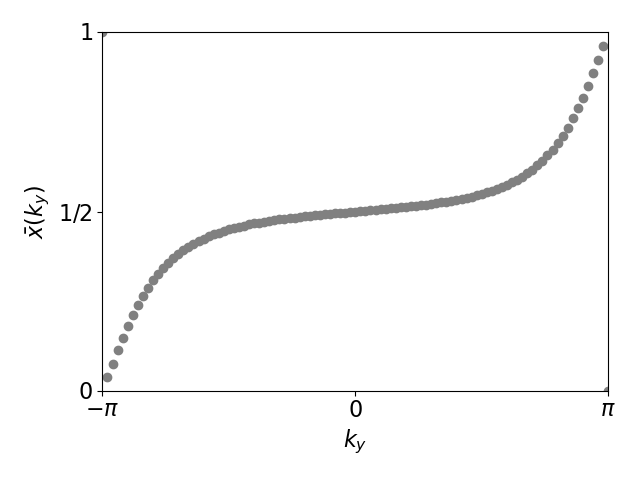
Figure 1: Wannier center charge (WCC) spectra for occupied valence band of eq. (2). Spectral flow of WCCs indicates a unit Chern number.

When the Berry gauge connection is Abelian, computation of the Wilson loop is equivalent to computation of the one-dimensional winding number, which in the Altland-Zirnbauer tableChiu et al. (2016); Qi and Zhang (2011); Ryu et al. (2010); Schnyder et al. (2008); Chiu et al. (2013); Morimoto and Furusaki (2013), is $\mathbb{Z}$ classified for class AIII insulators, such as the famous Su-Schreiffer-Heeger modelSu et al. (1979). If the Berry gauge connection is non-Abelian, as is the case for spinful insulators in class AII, the Wilson loop is instead $\mathbb{Z}_{2}$ valued. Importantly, this formalism has been extended to allow for the determination of bulk topological invarants in higher dimensions through computation of hyrbid WCCs. This is simply the computation of WCCs as a function of a transverse momenta. As an illustrative example, we consider a model of a Chern insulator on a square latticeLaughlin (1981); Thouless et al. (1982); Niu et al. (1985); Haldane (1988). The Bloch Hamiltonian takes the form,

$$H(\mathbf{k})/t=\sin k_{x}\sigma_{1}+\sin k_{y}\sigma_{2}+(\cos k_{x}+\cos k_{y}+1.5)\sigma_{3}$$ (2)

where $t$ has units of energy, $\sigma_{j=1,2,3}$ correspond to the three Pauli matrices and the lattice constant has been set to unity. This model supports a non-trivial Chern number, $\mathcal{C}=1$ which can be computed as,

$$\mathcal{C}=\frac{1}{2\pi}\int_{BZ}d^{2}kF_{xy}(\mathbf{k}),$$ (3)

where $F_{xy}(\mathbf{k})=\partial_{k_{x}}A_{y}-\partial_{k_{y}}A_{x}$ is the Abelian Berry curvature. Alternatively, the first Chern number can be computed using hybrid WCCs as,

$$\mathcal{C}=\frac{1}{a}\left(\sum_{n}\bar{x}_{n}(k_{y}=2\pi)-\sum_{n}\bar{x}_{n}(k_{y}=0)\right),$$ (4)

where $\bar{x}(k_{y})$ are the WCCs computed via integration along the $k_{x}$ axis as a function of the transverse momenta $k_{y}$ and the sum is over the occupied bands. Upon defining the Bloch Hamiltonian in the PyBinding package, we execute the calculation in the formalism of BerryEasy as,

⬇

import BerryEasy as be

vec=lambda t1, t2: [t1, t2, 0] #integation along k_{x} as funct. of k_{y}

ds=100 #discretizing integration into 100 steps

ds2=100 #discretize ky direction, 100 WCC computations will be performed

bands=[0] #Considering the occupied bands (can also use bands=range(1))

syst=chern_model #System we are considering is chern pybinding instance

WCCx=be.WSurf(vec,syst,bands,ds,ds2)

The results of the computation, shown in Fig. (1), detail that the WCCs smoothly interpolate between $0$ and $1$ as a function of $k_{y}$ indicating the Chern number $\mathcal{C}=1$.

It is now important to consider a spinful system supporting time-reversal symmetry $\mathcal{T}$ with $\mathcal{T}^{2}=-1$. In this case the system belongs to class AII and supports a $\mathbb{Z}_{2}$ topological invariant under the 10 fold classification scheme. Importantly, it was shown that a direct connection can be made between the $\mathbb{Z}_{2}$ indexFu and Kane (2007, 2006) and the WCC spectra in Ref. Yu et al. (2011). We briefly summarize that in a time-reversal symmetric system each Kramers pair is composed of two eigenstates which admit equal and opposite Chern numbers, $\mathcal{C}_{1}=-\mathcal{C}_{2}$. The $\mathbb{Z}_{2}$ index is then determined as, $\nu=(\mathcal{C}_{1}-\mathcal{C}_{2})/2\;\text{Mod}\;2$. As a result, a non-trivial $\mathbb{Z}_{2}$ index is indicated by the presence of a WCC spectra simultaneously detailing a smooth interpolation from $\bar{x}(0)=0(a)$ to $\bar{x}=a(0)$.

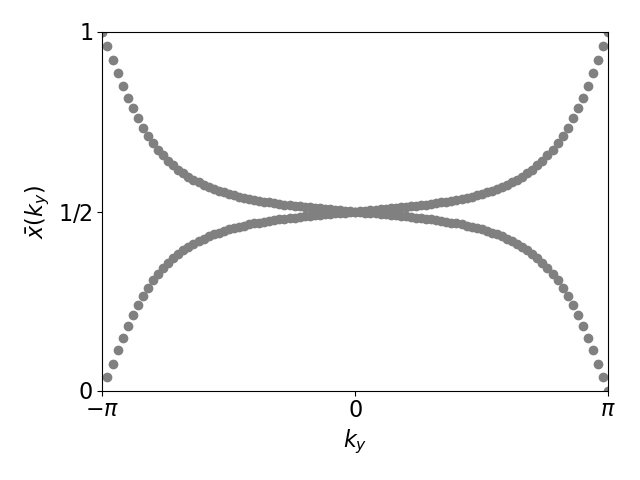
Figure 2: Wannier center charge (WCC) spectra for occupied valence band of eq. (5). Gapless nature of WCC spectra indicates a non-trivial $\mathbb{Z}_{2}$ index.

As an example of this behavior we will modify the Bloch Hamiltonian in eq. (2) to the form,

$$H(\mathbf{k})/t=\sin k_{x}\sigma_{1}\otimes\tau_{1}+\sin k_{y}\sigma_{1}\otimes\tau_{2}\\ +(\cos k_{x}+\cos k_{y}+1.5)\sigma_{3}\otimes\tau_{0},$$ (5)

where $\sigma_{0,1,2,3}(\tau_{0,1,2,3})$ are the $2\times 2$ identity matrix and three Pauli matrices respectively, operating on the spin (orbital) indices. This is the celebrated Bernevig-Hughes-Zhang modelBernevig et al. (2006); Qi et al. (2008) of the quantum spin-Hall insulator. Using the BerryEasy package, the WCC spectra is then computed as,

⬇

import BerryEasy as be

vec=lambda t1, t2: [t1, t2, 0] #integation along kx as funct. of ky

ds=100 #discretizing integration into 100 steps

ds2=100 #discretize ky direction, 100 WCC computations will be performed

bands=[0,1] #Considering the occupied bands (can also use bands=range(2))

syst=BHZ_model #System we are considering is BHZ pybinding instance

rvec=2*np.pi*np.diag(np.ones(3)) # specify reciprocal lattice

WCC=be.WSurf(vec,syst,bands,ds,ds2,rvec)

The results in Fig. (2) demonstrate the resulting fully connected WCC spectra indicating a non-trivial $\mathbb{Z}_{2}$ index. This formalism can be easily extended to three-dimensional systems as computation of the weak $\mathbb{Z}_{2}$ indices amounts to implementation of the two-dimensional computation in each high-symmetry plane, with the strong index the result of multiplying the weak indicesFu and Kane (2007).

II.1 Example: Topological Insulator with vacancies

As discussed in the introduction, a benefit of the PyBinding package is the capability to include fields and defects with ease. Accounting for defects is critical to the investigation of any realistic experimental setup but computing topological invariants in the presence of defects such as vacancies can be exceedingly challenging. In this example, we consider the BHZ model of a two-dimensional quantum spin-Hall insulator with a non-trivial $\mathbb{Z}_{2}$ indexBernevig et al. (2006); Qi et al. (2008). We will create a supercell of $21\times 21$ unit cells. We then remove lattice sites contained within a radius $r$ centered at the origin. As $r$ is increased the $\mathbb{Z}_{2}$ index will be computed. For a Jupyter notebook containing full details of this example please consult Ref. git .

Vacancies can be included in lattice tight-binding models simply in the PyBinding package through the use of the site-state modifier function. As stated we will consider a $21\times 21$ supercell of the model given in eq. (5). A plot of the supercell and bulk density of states for varying values of $r$ is shown in Fig. (LABEL:fig:dosvac) as well as images of the supercell with vacancies in Figs. (LABEL:fig:r1)-(LABEL:fig:r3). We note as $r$ is increased the density of states within the bulk gap begins to become populated. This can be understood in a straightforward manner: increasing $r$ causes the vacancies to appear as a boundary with edge states. The limited size of the boundary means the hybridization of these edge states maintains an energetic gap, protecting the bulk topology.

To test this, the $\mathbb{Z}_{2}$ index can be computed via the Wannier center charge spectra of the supercell in the presence of the vacancies. The results of this computation are available in Figs. (LABEL:fig:WCCr1)-(LABEL:fig:WCCr3), indicating that indeed the spectra remains gapless and the $\mathbb{Z}_{2}$ index is intact.

III Nested WCC spectra

There are currently limited community codes which accommodate computation of the nested Wilson loop. The nested Wilson loop or nested WCC spectra was introduced in Refs. Benalcazar et al. (2017, 2019); Schindler et al. (2018) as a method for computing the WCC spectra of the Wannier Hamiltonian. As an example, the Wannier Hamiltonian for a two-dimensional system takes the form, $H_{W1}(k_{2})$, computed as,

$$H_{W1}(k_{2})=\text{Im}\left(\text{Ln}\left(\mathcal{P}\text{exp}\left(i\int_{-\pi/a}^{\pi/a}dkA_{1}(k_{2})\right)\right)\right),$$ (6)

where $\mathcal{P}$ indicates path-ordering and $A_{1}(k_{2})$ is the Berry gauge connection for occupied bands. While claims that the Wannier Hamiltonian is equivalent to the surface Hamiltonian have been made to justify the use of the nested Wilson loop in diagnosis of higher-order topological insulators where the surfaces can take the form of lower dimensional topological insulators, this remains unresolved with counter examples appearing in the literatureChen et al. (2023).

Nevertheless, the nested Wilson loop has proven incredibly useful and powerful in diagnosing higher-order topological insulators (HOTIs). While the nested Wilson loop formalism is provided in detail in Ref. Benalcazar et al. (2017), here we provide an example for its implementation using the BerryEasy package. For clarity we will utilize the well studied chiral HOTI Bloch HamiltonianSchindler et al. (2018) which takes the form,

$$H(\mathbf{k})/t=\sin k_{x}\sigma_{1}\otimes\tau_{1}+\sin k_{y}\sigma_{1}\otimes\tau_{2}+\sin k_{z}\sigma_{1}\otimes\tau_{3}\\ +(\cos k_{x}+\cos k_{y}+1.5)\sigma_{3}\otimes\tau_{0}+\Delta_{0}(\cos k_{x}-\cos k_{y})\sigma_{2}\otimes\tau_{0}.$$ (7)

If $\Delta_{0}$ is set to zero we note that the model reduces to that of a strong topological insulator. However, by setting $\Delta_{0}=1$, the surface states are gapped on the $(100)$ and $(010)$ surfaces. As a result, the WCC spectra is gapped, as seen in Fig. (LABEL:fig:CHWCC). At this point we compute the nested WCC spectra as a function of $k_{z}$. In the BerryEasy package this performed as,

⬇

import BerryEasy as be

NL=[]

for kz in np.linspace(0,1,21):

vec=lambda t1, t2: [t1, t2, kz] #integation along kx as funct. of ky at kz=0

ds=100 #discretizing integration along k_{x} into 100 steps

ds2=100 #discretize integration along ky into 100 steps

bands=[0,1] #Considering the occupied bands (can also use bands=range(2))

syst=CHOTI_model #System we are considering is chiral HOTI pybinding instance

rvec=2*np.pi*np.diag(np.ones(3)) # specify reciprocal lattice

NL.append(be.WNWL(vec,syst,bands,ds,ds2,rvec))

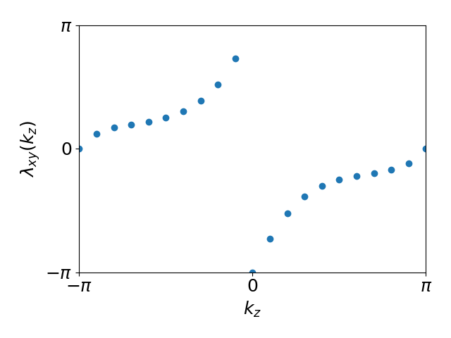
Figure 9: Spectra as a function of $k_{z}$ of Wannier Hamiltonian constructed via Wilson loop along the $k_{x}$ direction as a function of $k_{y}$, also known as nested Wilson loop.

The results seen in Fig. (9), demonstrate that the nested Wilson loop shows a gapless spectra indicating that the surface resembles a non-trivial Chern insulator with gapless chiral edge states. These edge states are the famous chiral hinge modes.

IV Spin-resolved WCC spectra

While first introduced by ProdanProdan (2009) over a decade previously, the spin-resolved Chern number ($\mathcal{C}_{s}$) has found renewed importance in the diagnosis of band topology for spinful higher-order and fragile topological insulators as the crystalline symmetry preserving perturbations which serve to gap the edge states and bring about higher-order topology often violate the spin-rotation symmetry, forcing the use of this method to diagnosis the bulk invariannt. The spin-resolved WCC spectra is detailed at length in Ref. Prodan (2009); Lin et al. (2022), where a python package for its computation within the PythTB package is provided. This is a terrific community code. Nevertheless, we have found a need for implementation of the spin-resolved Wilson loop for instances in PyBinding given the ease with which realistic fields and perturbations can be included. As an example, we again utilize the Bloch Hamiltonian given in eq. (7). As seen in the upper panel of Fig. (LABEL:fig:CHWCC), the WCC spectra is gapped. Computation of the spin-resolved WCC spectra requires defining the projected spin operator (PSO), $P(\mathbf{k})\hat{s}P(\mathbf{k})$, where $P(\mathbf{k})$ is the projector onto occupied bands and $\hat{s}$ is a chosen spin-quantization axis. In the absence of spin-orbit coupling the eigenvalues of the PSO are fixed as $\pm 1$, however since we have introduced spin-orbit coupling in eq. (7), the eigenvalues can adiabatically deviate from $\pm 1$. Nevertheless, a gap in the eigenvalue spectra of the PSO remains when selecting $\hat{s}=s_{z}=\sigma_{3}\otimes\tau_{3}$, allowing for calculation of the WCC spectra for the valence eigenstates of the PSO, $\bar{x}_{-}(k_{y})$ as detailed in Lin et. alLin et al. (2022). The results of this calculation fixing $k_{z}=\pi$ are seen in Fig. (LABEL:fig:CHSpinWCC), detailing the presence of a non-trivial spin-Chern number, $|\mathcal{C}_{s}|=1$.

This computation is performed in the BerryEasy package via the following lines of code:

⬇

import BerryEasy as be

vec=lambda t1, t2: [t1, t2, 0] #integation along kx as funct. of ky at kz=0

ds=100 #discretizing integration into 100 steps

ds2=100 #discretize ky direction, 100 WCC computations will be performed

bands=[0,1] #Considering the occupied bands (can also use bands=range(2))

syst=CHOTI_model #System we are considering is chiral HOTI pybinding instance

rvec=2*np.pi*np.diag(np.ones(3)) # specify reciprocal lattice

op=np.diag([1,-1,-1,1]) #Define prefered spin axis

WS=be.WSpinSurf(vec,model,bnds,ds,ds2,op,rvec)

IV.1 Example: Disordered quadrupolar insulator

The study of disorder in topological quantum matter is of supreme importance yet it presents a computational challengeHaldane (1988); Sheng et al. (2006); Onoda et al. (2007); Obuse et al. (2008); Prodan et al. (2010). In order to demonstrate the benefits of the BerryEasy program and its integration with the PyBinding package, we consider the case of a disordered quadrupolar insulatorBenalcazar et al. (2017). Disorder is generally difficult to implement in the alternative packages listed previously, however, here we show that PyBinding’s built in on-site modifiers combined with the BerryEasy package allow for an efficient route to establishing bulk topological invariants in disordered systems. We will consider a spinful version of the celebrated Benalcazar-Bernevig-Hughes modelBenalcazar et al. (2017), the Bloch Hamiltonian is given as,

$$H(\mathbf{k})/t=\sin k_{x}\sigma_{1}\otimes\tau_{3}+\sin k_{y}\sigma_{2}\otimes\tau_{3}\\ +(\cos k_{x}+\cos k_{y}+1)\sigma_{3}\otimes\tau_{3}\\ +0.5(\cos k_{x}-\cos k_{y})\sigma_{0}\otimes\tau_{0}.$$ (8)

This Hamiltonian supports chiral symmetry, generated as $S^{-1}HS=-H$, where $S=\sigma_{0}\otimes\tau_{2}$. In Refs. Li et al. (2020); Hu et al. (2021); Yang et al. (2021), the robustness of the bulk topology to chiral symmetry preserving disorder was studied in depth. It was shown that the bulk spin-Chern number, as defined using the method of ProdanProdan (2009) fixing $\hat{s}=\sigma_{0}\otimes\tau_{3}$ in the PSO, was robust prior to the closing of the average bulk energetic gap. Following Ref. Hu et al. (2021), this disorder will be implemented as $H_{dis}=\{w_{1},w_{1}\}\otimes\tau_{3}$, where $w_{j}$ is selected randomly from a uniform distribution, $[-W/2,W/2)$. The bulk average density of states can be calculated rapidly for a $100\times 100$ system using the built-in Kernel Polynomial Method (KPM) solvers in PyBinding, averaging over 100 disorder configurations (for a Jupyter Notebook detailing this example please consult Ref. git ). The results shown in Fig. (LABEL:fig:AvgDOS) demonstrate that the average bulk gap remains open until $W\approx 5$. In order to determine the spin-Chern number in the presence of disorder we first create a supercell of size $21\times 21$ lattice cells and apply the chiral-symmetry preserving disorder. We then impose periodic boundary conditions such that the $21\times 21$ system represents the fundamental unit cell and the reciprocal lattice vectors are altered as $2\pi\rightarrow 2\pi/(21a)$, where $a$ is the lattice constant which we set to unity. As we are working with a supercell, the reciprocal lattice vectors and the number of valence bands must be modified to account for the increase in the dimensions of the Bloch Hamiltonian. We then perform the spin-Chern number computation. This is accomplished utilizing the $WSpinLine$ function in BerryEasy, which allows for explicit construction of closed lines in momentum space along which the Wilson loop is computed. These closed paths are constructed by discretizing the Brillouin zone into a grid of $20\times 20$ plaquettes for which the integrated Berry flux is computed and averaged over 20 disorder configurations. The results shown in Fig. (LABEL:fig:DisSC), demonstrate that the spin-Chern number remains intact prior to closing of the average bulk gap. A sample output of this computation in the region before and after closing of the bulk gap is shown in Figs. (LABEL:fig:Cs1) and (LABEL:fig:Cs0) respectively.

IV.1.1 GPU utilization to expedite calculations:

The effects of disorder in solid-state systems admitting non-trivial band topology continues to be an area of active research. In general, the bulk topological invariant is robust to the introduction of disorder which leaves the bulk mobility gap intact. However, measurement of the bulk topological invariant in disordered systems is known to be a computationally demanding endeavor due to the need to simultaneously avoid finite size effects and average over many disorder configurations.

In this example, we have showcased the ability of BerryEasy package to compute the spin-resolved Chern number, a capability offered by only one other community code, and to perform the computation rapidly in a large supercell accounting for disorder utilizing the power of GPUs. In Fig. (LABEL:fig:Comp), we plot the time for computing integrated Berry flux for the occupied states of eq. (8) through a single plaquette in an $L\times L$ supercell of the BerryEasy package when utilizing a Tesla V100 GPU vs Intel-Xeon CPU as offered in Google Colab. The figure demonstrates the enormous speed advantage of GPU evaluation. In Fig. (LABEL:fig:BeLog), it is shown that for $L>5$, the speed advantage is significant. This is of vital importance to achieve accurate results as finite size effects can be minimized and a greater number of disorder configurations can be considered without requiring extended computational time. The code utilized for the results in Fig. (LABEL:fig:Disorder) is available on githubgit .

V Wannier90 tight-binding models

Finally, progress in the diagnosis of band topology has been accelerated by the ability to directly utilize the tools listed above in realistic tight-binding models derived from density functional theory data using the Wannier90 software package. A primary advantage of the PythTB, Z2Pack and WannierTools software packages is their ability to directly interface with the output of Wannier90 for construction of a tight-binding model from which topological quantities can be computed using the built in functionalities. The BerryEasy package provides a built-in version of wanPBwan to create PyBinding instances from the output of Wannier90, thereby extending the functionality of the tools detailed above to realistic many-band models generated from density functional theory.

As an example, we examine a known $\mathbb{Z}_{2}$ topological insulator in two-dimensions, bilayer-bismuthWada et al. (2011); Murakami (2006); Tyner and Goswami (2023), also known as $\beta$-bismuthene. All first principles calculations based on density-functional theory (DFT) are carried out using the Quantum Espresso software package Giannozzi et al. (2009, 2017, 2020). Exchange-correlation potentials use the Perdew-Burke-Ernzerhof (PBE) parametrization of the generalized gradient approximation (GGA) Perdew et al. (1997). The self-consistent and non-self consistent computations are performed using a $40\times 40\times 1$ Monkhorst-Pack grid and a cutoff of 100 Ry. We implement norm-conserving pseudo-potentialsHamann (2013) as obtained on the Pseudo-Dojo sitevan Setten et al. (2018). Spin-orbit coupling is consider in all calculations. The Wannier tight-binding model was constructed using the Wannier90 software package. The necessary input and output files are available publiclygit . Utilizing the Bi_tb.dat and Bi_centres.xyz files, we create the PyBinding tight-binding model using the following function to create the lattice and save it,

⬇

import BerryEasy as be

ECut=0.05 #cutoff for hopping strength

HopCut=100 #hopping neighbors cutoff

seedname=str(Bi)

lat = be.wan90_lat(ECut,HopCut,seedname)

pb.save(lat,”BiWTB.pbz”)

Upon plotting the band structure seen in Fig. (LABEL:fig:BiBands), we investigate the nature of the ground state topology using the built-in function for computing WCCs. Besides specifying the correct number of valence bands and the correct reciprocal lattice vectors, the necessary code is virtually unchanged from that displayed for eq. (5). The results are then plotted showing that the hybrid WCC spectra is gapless in Fig. (LABEL:fig:BEWCCBi). As such the system can be classified as a strong topological insulator. While such a computation can be performed using any of the software packages given previously (this is demonstrated by comparing the results to those obtained by the Z2Pack software package to show that they are identical in Fig. (LABEL:fig:Z2WCCBi)), we remark that the ability to implement perturbations such as disorder or impurities now remains possible even in the context of complicated Wannier tight-binding models through the interface with PyBinding.

VI Summary

In summary, multiple excellent community codes currently exist for the computation of topological quantities in both Wannier tight-binding models and idealized toy models. However, each package is ideally suited to different use cases. The BerryEasy package fills what we view as a current gap in this spectra of offerings by providing access to state-of-the-art diagnostics for toy models and realistic models while simultaneously offering the possibility to account for application of fields and effects by interfacing with the PyBinding package. As a result, it is our hope that this package will prove useful both for those researchers investigating new forms of topological order in clean systems as well as those interested in understanding the complex effects of disorder and application of external fields in realistic systems being actively studied in experimental settings. Future versions of the BerryEasy package are currently being developed to accommodate tight-binding models defined using TBModelsGresch et al. (2017) and KwantGroth et al. (2014).

- (1) https://www.physics.rutgers.edu/pythtb/index.html.
- Moldovan et al. (2020) D. Moldovan, M. Andelković, and F. Peeters, Version v0 9 (2020).
- Tang et al. (2019a) F. Tang, H. C. Po, A. Vishwanath, and X. Wan, Nat. Phys. 15, 470 (2019a).
- Zhang et al. (2019) T. Zhang, Y. Jiang, Z. Song, H. Huang, Y. He, Z. Fang, H. Weng, and C. Fang, Nature 566, 475 (2019).
- Vergniory et al. (2019) M. Vergniory, L. Elcoro, C. Felser, N. Regnault, B. A. Bernevig, and Z. Wang, Nature 566, 480 (2019).
- Tang et al. (2019b) F. Tang, H. C. Po, A. Vishwanath, and X. Wan, Nature 566, 486 (2019b).
- Xu et al. (2020) Y. Xu, L. Elcoro, Z.-D. Song, B. J. Wieder, M. Vergniory, N. Regnault, Y. Chen, C. Felser, and B. A. Bernevig, Nature 586, 702 (2020).
- Gresch et al. (2017) D. Gresch, G. Autès, O. V. Yazyev, M. Troyer, D. Vanderbilt, B. A. Bernevig, and A. A. Soluyanov, Phys. Rev. B 95, 075146 (2017).
- Wu et al. (2018) Q. Wu, S. Zhang, H.-F. Song, M. Troyer, and A. A. Soluyanov, Comput. Phys. Commun. 224, 405 (2018).
- Pizzi et al. (2020) G. Pizzi, V. Vitale, R. Arita, S. Blugel, F. Freimuth, G. Géranton, M. Gibertini, D. Gresch, C. Johnson, T. Koretsune, J. Ibañez-Azpiroz, H. Lee, J.-M. Lihm, D. Marchand, A. Marrazzo, Y. Mokrousov, J. I. Mustafa, Y. Nohara, Y. Nomura, L. Paulatto, S. Poncé, T. Ponweiser, J. Qiao, F. Thole, S. S. Tsirkin, M. Wierzbowska, N. Marzari, D. Vanderbilt, I. Souza, A. A. Mostofi, and J. R. Yates, J. Phys. Condens. Matter 32, 165902 (2020).
- Groth et al. (2014) C. W. Groth, M. Wimmer, A. R. Akhmerov, and X. Waintal, New J. Phys. 16, 063065 (2014).
- Tsirkin (2021) S. S. Tsirkin, npj Computational Materials 7, 1 (2021).
- Benalcazar et al. (2017) W. A. Benalcazar, B. A. Bernevig, and T. L. Hughes, Science 357, 61 (2017).
- Schindler et al. (2018) F. Schindler, A. M. Cook, M. G. Vergniory, Z. Wang, S. S. P. Parkin, B. A. Bernevig, and T. Neupert, Sci. Adv. 4 (2018), 10.1126/sciadv.aat0346.
- Prodan (2009) E. Prodan, Phys. Rev. B 80, 125327 (2009).
- Lin et al. (2022) K.-S. Lin, G. Palumbo, Z. Guo, J. Blackburn, D. Shoemaker, F. Mahmood, Z. Wang, G. Fiete, B. Wieder, and B. Bradlyn, arXiv:2207.10099 (2022).
- Marzari and Vanderbilt (1997) N. Marzari and D. Vanderbilt, Phys. Rev. B 56, 12847 (1997).
- Brouder et al. (2007) C. Brouder, G. Panati, M. Calandra, C. Mourougane, and N. Marzari, Phys. Rev. Lett. 98, 046402 (2007).
- Coh and Vanderbilt (2009) S. Coh and D. Vanderbilt, Phys. Rev. Lett. 102, 107603 (2009).
- Yu et al. (2011) R. Yu, X. L. Qi, A. Bernevig, Z. Fang, and X. Dai, Phys. Rev. B 84, 075119 (2011).
- Soluyanov and Vanderbilt (2011a) A. A. Soluyanov and D. Vanderbilt, Phys. Rev. B 83, 235401 (2011a).
- Soluyanov and Vanderbilt (2011b) A. A. Soluyanov and D. Vanderbilt, Phys. Rev. B 83, 035108 (2011b).
- Alexandradinata et al. (2014) A. Alexandradinata, X. Dai, and B. A. Bernevig, Phys. Rev. B 89, 155114 (2014).
- Taherinejad et al. (2014) M. Taherinejad, K. F. Garrity, and D. Vanderbilt, Phys. Rev. B 89, 1 (2014), 1312.6940 .
- Bouhon et al. (2019) A. Bouhon, A. M. Black-Schaffer, and R.-J. Slager, Phys. Rev. B 100, 195135 (2019).
- Bradlyn et al. (2019) B. Bradlyn, Z. Wang, J. Cano, and B. A. Bernevig, Phys. Rev. B 99, 045140 (2019).
- Okuta et al. (2017) R. Okuta, Y. Unno, D. Nishino, S. Hido, and C. Loomis, in Proceedings of Workshop on Machine Learning Systems (LearningSys) in The Thirty-first Annual Conference on Neural Information Processing Systems (NIPS) (2017).
- Chiu et al. (2016) C.-K. Chiu, J. C. Y. Teo, A. P. Schnyder, and S. Ryu, Rev. Mod. Phys. 88, 035005 (2016).
- Qi and Zhang (2011) X.-L. Qi and S.-C. Zhang, Rev. Mod. Phys. 83, 1057 (2011).
- Ryu et al. (2010) S. Ryu, A. P. Schnyder, A. Furusaki, and A. W. Ludwig, New J. Phys. 12, 065010 (2010).
- Schnyder et al. (2008) A. P. Schnyder, S. Ryu, A. Furusaki, and A. W. W. Ludwig, Phys. Rev. B 78, 195125 (2008).
- Chiu et al. (2013) C.-K. Chiu, H. Yao, and S. Ryu, Phys. Rev. B 88, 075142 (2013).
- Morimoto and Furusaki (2013) T. Morimoto and A. Furusaki, Phys. Rev. B 88, 125129 (2013).
- Su et al. (1979) W. P. Su, J. R. Schrieffer, and A. J. Heeger, Phys. Rev. Lett. 42, 1698 (1979).
- Laughlin (1981) R. B. Laughlin, Phys. Rev. B 23, 5632 (1981).
- Thouless et al. (1982) D. J. Thouless, M. Kohmoto, M. P. Nightingale, and M. den Nijs, Phys. Rev. Lett. 49, 405 (1982).
- Niu et al. (1985) Q. Niu, D. J. Thouless, and Y.-S. Wu, Phys. Rev. B 31, 3372 (1985).
- Haldane (1988) F. D. M. Haldane, Phys. Rev. Lett. 61, 2015 (1988).
- Fu and Kane (2007) L. Fu and C. L. Kane, Phys. Rev. B 76, 045302 (2007).
- Fu and Kane (2006) L. Fu and C. L. Kane, Phys. Rev. B 74, 195312 (2006).
- Bernevig et al. (2006) B. A. Bernevig, T. L. Hughes, and S.-C. Zhang, Science 314, 1757 (2006).
- Qi et al. (2008) X.-L. Qi, T. L. Hughes, and S.-C. Zhang, Phys. Rev. B 78, 195424 (2008).
- (43) https://github.com/actyner/BerryEasy.
- Benalcazar et al. (2019) W. A. Benalcazar, T. Li, and T. L. Hughes, Phys. Rev. B 99, 245151 (2019).
- Chen et al. (2023) Y.-C. Chen, Y.-P. Lin, and Y.-J. Kao, Phys. Rev. B 107, 075126 (2023).
- Sheng et al. (2006) D. N. Sheng, Z. Y. Weng, L. Sheng, and F. D. M. Haldane, Phys. Rev. Lett. 97, 036808 (2006).
- Onoda et al. (2007) M. Onoda, Y. Avishai, and N. Nagaosa, Phys. Rev. Lett. 98, 076802 (2007).
- Obuse et al. (2008) H. Obuse, A. Furusaki, S. Ryu, and C. Mudry, Phys. Rev. B 78, 115301 (2008).
- Prodan et al. (2010) E. Prodan, T. L. Hughes, and B. A. Bernevig, Phys. Rev. Lett. 105, 115501 (2010).
- Li et al. (2020) C.-A. Li, B. Fu, Z.-A. Hu, J. Li, and S.-Q. Shen, Phys. Rev. Lett. 125, 166801 (2020).
- Hu et al. (2021) Y.-S. Hu, Y.-R. Ding, J. Zhang, Z.-Q. Zhang, and C.-Z. Chen, Phys. Rev. B 104, 094201 (2021).
- Yang et al. (2021) Y.-B. Yang, K. Li, L.-M. Duan, and Y. Xu, Phys. Rev. B 103, 085408 (2021).
- (53) https://github.com/Chengcheng-Xiao/wanPB.
- Wada et al. (2011) M. Wada, S. Murakami, F. Freimuth, and G. Bihlmayer, Phys. Rev. B 83, 121310 (2011).
- Murakami (2006) S. Murakami, Phys. Rev. Lett. 97, 236805 (2006).
- Tyner and Goswami (2023) A. C. Tyner and P. Goswami, Sci. Rep. 13, 11393 (2023).
- Giannozzi et al. (2009) P. Giannozzi, S. Baroni, N. Bonini, M. Calandra, R. Car, C. Cavazzoni, D. Ceresoli, G. L. Chiarotti, M. Cococcioni, I. Dabo, A. Dal Corso, S. de Gironcoli, S. Fabris, G. Fratesi, R. Gebauer, U. Gerstmann, C. Gougoussis, A. Kokalj, M. Lazzeri, L. Martin-Samos, N. Marzari, F. Mauri, R. Mazzarello, S. Paolini, A. Pasquarello, L. Paulatto, C. Sbraccia, S. Scandolo, G. Sclauzero, A. P. Seitsonen, A. Smogunov, P. Umari, and R. M. Wentzcovitch, J. Phys. Condens. Matter 21, 395502 (19pp) (2009).
- Giannozzi et al. (2017) P. Giannozzi, O. Andreussi, T. Brumme, O. Bunau, M. B. Nardelli, M. Calandra, R. Car, C. Cavazzoni, D. Ceresoli, M. Cococcioni, N. Colonna, I. Carnimeo, A. D. Corso, S. de Gironcoli, P. Delugas, R. A. D. Jr, A. Ferretti, A. Floris, G. Fratesi, G. Fugallo, R. Gebauer, U. Gerstmann, F. Giustino, T. Gorni, J. Jia, M. Kawamura, H.-Y. Ko, A. Kokalj, E. Küçükbenli, M. Lazzeri, M. Marsili, N. Marzari, F. Mauri, N. L. Nguyen, H.-V. Nguyen, A. O. de-la Roza, L. Paulatto, S. Poncé, D. Rocca, R. Sabatini, B. Santra, M. Schlipf, A. P. Seitsonen, A. Smogunov, I. Timrov, T. Thonhauser, P. Umari, N. Vast, X. Wu, and S. Baroni, J. Phys. Condens. Matter 29, 465901 (2017).
- Giannozzi et al. (2020) P. Giannozzi, O. Baseggio, P. Bonfà, D. Brunato, R. Car, I. Carnimeo, C. Cavazzoni, S. de Gironcoli, P. Delugas, F. Ferrari Ruffino, A. Ferretti, N. Marzari, I. Timrov, A. Urru, and S. Baroni, J. Chem. Phys. 152, 154105 (2020).
- Perdew et al. (1997) J. P. Perdew, K. Burke, and M. Ernzerhof, Phys. Rev. Lett. 78, 1396 (1997).
- Hamann (2013) D. R. Hamann, Phys. Rev. B 88, 085117 (2013).
- van Setten et al. (2018) M. J. van Setten, M. Giantomassi, E. Bousquet, M. J. Verstraete, D. R. Hamann, X. Gonze, and G.-M. Rignanese, Comput. Phys. Commun. 226, 39 (2018).