Impact of Correlations on the Modeling and Inference of Beyond Vacuum-GR Effects in Extreme-Mass-Ratio Inspirals

Abstract

In gravitational-wave astronomy, extreme-mass-ratio-inspiral (EMRI) sources for the upcoming LISA observatory have the potential to serve as high-precision probes of astrophysical environments in galactic nuclei, and of potential deviations from general relativity (GR). Such “beyond vacuum-GR” effects are often modeled as perturbations to the evolution of vacuum EMRIs under GR. Previous studies have reported unprecedented constraints on these effects by examining the inference of one effect at a time. However, a more realistic analysis would require the simultaneous inference of multiple beyond vacuum-GR effects. The parameters describing such effects are generally significantly correlated with each other and the vacuum EMRI parameters. We explicitly show how these correlations remain even if any modeled effect is absent in the actual signal, and how they cause inference bias when any effect in the signal is absent in the analysis model. This worsens the overall measurability of the whole parameter set, challenging the constraints found by previous studies, and posing a general problem for the modeling and inference of beyond vacuum-GR effects in EMRIs.

Introduction.

EMRIs are binary systems comprising a stellar-mass compact object (CO) of mass $\mu\sim 1-10^{2}M_{\odot}$ and a massive black hole (MBH) of mass $M\sim 10^{5}-10^{7}M_{\odot}$ (Amaro-Seoane et al., 2015; Barack and Cutler, 2004). When such systems are in the strong-gravity regime (orbital separation $r\sim 10GM/c^{2}$), they will produce gravitational-wave (GW) signals in the millihertz frequency band of the upcoming space-based ESA-NASA observatory LISA (Seoane et al., 2013, 2017, 2012a, 2012b). EMRI source parameters can be constrained to sub-percent precision by LISA, which potentially enables stringent tests of GR and the measurement of beyond vacuum-GR effects caused by modified gravity or astrophysical environments Amaro-Seoane et al. (2007); Amaro-Seoane (2018); Gair et al. (2013); Babak et al. (2017); Berry et al. (2019); Chamberlain and Yunes (2017); Wang et al. (2022); Barausse et al. (2016); Yunes et al. (2010); Barbieri et al. (2023); Cardoso et al. (2011); Barsanti et al. (2023); Yunes et al. (2012); Barausse et al. (2014); Kocsis et al. (2011); Yunes et al. (2011); Zwick et al. (2023); Rahman et al. (2023); Speri et al. (2023).

Current state-of-the-art EMRI waveforms are modeled using black hole perturbation theory and self-force theory, where the Einstein field equations are solved by treating the gravitational field of the CO as a perturbation to the Kerr spacetime of the central MBH Pound and Wardell (2021); Barack and Pound (2018). At leading order in the mass ratio $\mu/M$, this approach reduces approximately to a set of flux equations describing the long-term evolution of the system Teukolsky (1973); Hinderer and Flanagan (2008); Fujita and Shibata (2020); Isoyama et al. (2022); Hughes et al. (2021). A beyond vacuum-GR effect may then be introduced by directly solving the field equations with the system’s stress-energy tensor altered by this effect, or by including the expected modifications due to the effect at the level of the fluxes (or the waveform itself). The latter approach is far more popular in the literature, due to its greater simplicity.

In flux-based models, the flux equations modified by a beyond vacuum-GR effect take the general form

$$\dot{E} =\dot{E}_{\mathrm{GR}}(\boldsymbol{\psi})\left(1+A(\alpha)\mathcal{F}(\boldsymbol{\psi},\boldsymbol{\phi})\right),$$ (1)

$$\dot{L} =\dot{L}_{\mathrm{GR}}(\boldsymbol{\psi})\left(1+B(\alpha)\mathcal{G}(\boldsymbol{\psi},\boldsymbol{\phi})\right),$$ (2)

where $\dot{E}_{\mathrm{GR}},\dot{L}_{\mathrm{GR}}$ are the leading-order vacuum-GR fluxes that depend only on the vacuum-GR parameter vector $\boldsymbol{\psi}$, while $A\mathcal{F},B\mathcal{G}$ are the perturbative corrections induced by the beyond vacuum-GR effect. Here, $A,B$ are the effect amplitudes, which in general are functions of an underlying amplitude parameter $\alpha$ (such that $A,B\to 0$ as $\alpha\to 0$). The remaining functional dependence of the effect on any non-amplitude effect parameters $\boldsymbol{\phi}$ is contained in $\mathcal{F},\mathcal{G}$, which may also depend on $\boldsymbol{\psi}$. These modified fluxes are then used in GR waveform models $h(\dot{E},\dot{L})$ to generate beyond vacuum-GR waveforms (with the implicit assumption that the effect does not modify the dependence of $h$ itself on $\dot{E},\dot{L}$).

Most studies of modified-gravity and environmental effects on EMRIs adopt this general framework. For example, Chamberlain et al. Chamberlain and Yunes (2017) found that the effect of GW dipole radiation predicted by some scalar-tensor modified gravity theories Blanchet (2006); Will (2006); Brans and Dicke (1961); Will (1993) (which perturbs the vacuum-GR energy flux as $\dot{E}=\dot{E}_{\mathrm{GR}}\left(1+Bp^{n_{\mathrm{dip}}}\right)$ Barausse et al. (2016) with $p\equiv p(\boldsymbol{\psi}),B\equiv\alpha,n_{\mathrm{dip}}\equiv\boldsymbol{\phi}$) can be constrained by LISA to a precision several orders of magnitude better than current ground-based GW detectors. More recently, Speri et al. Speri et al. (2023) found that the planetary migration torque of a thin accretion disk surrounding an EMRI (which modifies the angular momentum flux as $\dot{L}=\dot{L}_{\mathrm{GR}}\left(1+A\left(p/10\right)^{n}\right)$ Barausse et al. (2014); Kocsis et al. (2011) with $p\equiv p(\boldsymbol{\psi}),A\equiv\alpha,n\equiv\boldsymbol{\phi}$) is measurable by LISA to $\sim 10\%$ precision. Many other examples that set similarly tight constraints on beyond vacuum-GR effects can be found in the literature, e.g., Yunes et al. (2010, 2011); Cardoso et al. (2011); Barsanti et al. (2023); Yunes et al. (2012); Barausse et al. (2014); Kocsis et al. (2011).

The use of flux corrections with the power-law form $Ap^{n}$ (where $p$ is the evolving dimensionless separation of the orbit) implicitly treats the effect in an orbit-averaged way, i.e., the manifestation of the effect on the timescale of orbital motion is neglected, and the accumulated effect is described on the longer radiation-reaction timescale as a secular “drift” from vacuum-GR orbital evolution. The power-law form enables one to gauge the post-Newtonian (PN) order at which the effect becomes relevant (through $n$), and its strength with respect to the vacuum-GR evolution (through $A$). Power-law corrections are also used in the parameterized post-Einsteinian (ppE) formalism Yunes and Pretorius (2009); Tahura and Yagi (2018), in which the beyond vacuum-GR corrections are made at the level of the waveform instead. We return to the ppE formalism in the discussion section.

While most current studies set constraints on beyond vacuum-GR effects in isolation, a more realistic analysis would have to account for the presence of multiple effects in a given source and to address the prospects of their simultaneous inference. For example, Wang et al. Wang et al. (2022) examined the joint inference of dipole GW radiation and a time-evolving Newton’s constant, which can both be present in modified gravity theories such as the Jordan-Fierz-Brans-Dicke theory Jordan and Schücking (1955); Fierz (1956); Brans and Dicke (1961). In the case of astrophysical environments, complex phenomena such as accretion disks will have multiple degrees of freedom that can give rise to different effects in a single source Kocsis et al. (2011). However, the joint inference of multiple effects is generically susceptible to several fundamental challenges, especially since most effects are modeled as small and simply described perturbations to the vacuum-GR solutions.

In this Letter, through a completely general framework, we demonstrate some of these challenges by using the Fisher information matrix (FIM) of the standard GW parameter likelihood to examine the impact of parameter correlations in beyond vacuum-GR modeling and inference. We illustrate our results with a taxonomy of representative cases, comment on their consequences for various themes in EMRI modeling and inference, and discuss possible ways to minimize their impact on the science output of EMRI observations with LISA.

General results.

Our analysis considers two broad cases: Case i@, where the GW signal lies in the template manifold $\mathcal{T}$ (the image space of the analysis waveform model), and Case ii@, where it does not. The signal $s$ itself is assumed to lie in a putative signal manifold $\mathcal{S}$ (the true space of actual signals). Case i@ has the subcases $\mathcal{S}\subseteq\mathcal{T}$ (e.g., a null test of GR; left panel of Fig. 1) and $\mathcal{S}\not\subseteq\mathcal{T}$ (e.g., a mismodeled null test), while Case ii@ has the subcases $\mathcal{T}\subset\mathcal{S}$ (e.g., a neglected effect; right panel of Fig. 1) and $\mathcal{T}\not\subset\mathcal{S}$ (e.g., a mismodeled effect). Case ii@ leads generically to bias and multimodality in inference, with the posterior modes corresponding to any template whose difference from $s$ is orthogonal to $\mathcal{T}$ Cutler and Vallisneri (2007); Chua (2020); Chua and Cutler (2022).

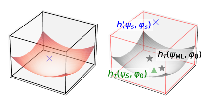
Figure 1: A schematic depiction of Case i@ with $\mathcal{S}\subset\mathcal{T}$ (left) and Case ii@ with $\mathcal{T}\subset\mathcal{S}$ (right). Red and black indicate $\mathcal{S}$ and $\mathcal{T}$ respectively, while the blue crosses represent the true signal $s$, the black stars are the posterior-mode templates, and the green triangle is the template that shares the signal parameters restricted to $\mathcal{T}$. Notation is defined in the text.

In both cases, there exists an ambient manifold $\mathcal{A}$ such that $\mathcal{T}\subseteq\mathcal{A}$ and $\mathcal{S}\subseteq\mathcal{A}$. We consider the putative waveform model $h(\boldsymbol{\theta})$ whose image space is $\mathcal{A}$, and the corresponding GW likelihood $\mathcal{L}(\boldsymbol{\theta}|s)=\exp{-1/2\langle s-h(\boldsymbol{\theta})|s-h(\boldsymbol{\theta})\rangle}$ (where $\left<\cdot|\cdot\right>$ is the standard detector-noise-weighted inner product on the data space of fixed-length time series Barack and Cutler (2004)). The FIM of $\mathcal{L}$ can be written in terms of waveform derivatives as Vallisneri (2008)

$$\Gamma_{ij}(\boldsymbol{\theta})= \left.\left<\tfrac{\partial h}{\partial\theta_{i}}\right|\tfrac{\partial h}{\partial\theta_{j}}\right>$$

$$= \left.\left<\tfrac{\partial h}{\partial\dot{E}}\tfrac{\partial\dot{E}}{\partial\theta_{i}}+\tfrac{\partial h}{\partial\dot{L}}\tfrac{\partial\dot{L}}{\partial\theta_{i}}\right|\tfrac{\partial h}{\partial\dot{E}}\tfrac{\partial\dot{E}}{\partial\theta_{j}}+\tfrac{\partial h}{\partial\dot{L}}\tfrac{\partial\dot{L}}{\partial\theta_{j}}\right>,$$ (3)

evaluated at the maximum-likelihood estimate $\boldsymbol{\theta}_{\mathrm{ML}}$. The inverse FIM $\Sigma=\Gamma^{-1}$ is then by definition the covariance matrix of the normal approximation to $\mathcal{L}$.

We first examine Case i@ with $\mathcal{S}\subseteq\mathcal{T}$, such that $\mathcal{A}\equiv\mathcal{T}$ and $s=h(\boldsymbol{\theta}_{\mathrm{ML}})$. The subcase $\mathcal{S}\not\subseteq\mathcal{T}$ requires the restriction of all quantities to $\mathcal{T}$, but is otherwise identical. As a representative example, we consider a flux-based EMRI model modified by two beyond vacuum-GR effects:

$$\dot{E} =\dot{E}_{\mathrm{GR}}(\boldsymbol{\psi})\left(1+\Sigma_{k=1}^{2}A_{k}(\alpha_{k})\mathcal{F}_{k}(\boldsymbol{\psi},\boldsymbol{\phi_{k}})\right),$$ (4)

$$\dot{L} =\dot{L}_{\mathrm{GR}}(\boldsymbol{\psi})\left(1+\Sigma_{k=1}^{2}B_{k}(\alpha_{k})\mathcal{G}_{k}(\boldsymbol{\psi},\boldsymbol{\phi_{k}})\right),$$ (5)

which yields the corresponding FIM $\Gamma(\boldsymbol{\psi},\alpha_{1},\boldsymbol{\phi}_{1},\alpha_{2},\boldsymbol{\phi}_{2})$. We focus on the vanishing of the second effect in the signal ($\alpha_{2}\to 0$ in $s$). When $\alpha_{2}=0$, the FIM is singular as the rows and columns corresponding to the components of $\boldsymbol{\phi}_{2}$ are zero, and $\boldsymbol{\phi}_{2}$ is unmeasurable. Equivalently, the precisions $(\Sigma_{\phi_{2}\phi_{2}})^{1/2}$ to which $\boldsymbol{\phi}_{2}$ can be measured blow up as $\alpha_{2}\to 0$. However, we show that See Supplemental Material at [URL will be inserted by publisher] for “Correlations between parameters of a beyond vacuum-GR EMRI do not vanish if an effect is absent”. all correlation coefficients $\rho_{ij}\equiv\Sigma_{ij}/(\Sigma_{ii}\Sigma_{jj})^{1/2}$ (including with $\boldsymbol{\phi_{2}}$) are $\mathcal{O}(1)$ and thus non-vanishing as $\alpha_{2}\to 0$. This result is valid generically, i.e., even if $A_{2},B_{2}$ (and their derivatives $A_{2}^{\prime},B_{2}^{\prime}$, if applicable) vanish at different rates. The non-vanishing correlations of all other parameters with $\boldsymbol{\phi}_{2}$ imply that their inference is also generally degraded in proportion to these correlations as $\alpha_{2}\to 0$.

Correlations between parameters also significantly impact inference in Case ii@, where the signal contains an effect that is neglected or mismodeled. We restrict to the subcase $\mathcal{T}\subset\mathcal{S}$ for simplicity, such that $\mathcal{A}\equiv\mathcal{S}$, and partition the parameters $\boldsymbol{\theta}$ more generally as $(\boldsymbol{\psi},\boldsymbol{\varphi})$, where the $\boldsymbol{\varphi}$ describe an effect that vanishes for some values $\boldsymbol{\varphi}_{0}$. The signal is $s=h(\boldsymbol{\psi}_{s},\boldsymbol{\varphi}_{s})\not\in\mathcal{T}$, for some $\boldsymbol{\varphi}_{s}\neq\boldsymbol{\varphi}_{0}$. Note that the analysis waveform model is now not $h\equiv h_{\mathcal{S}}$ but its restriction to $\mathcal{T}$, i.e., $h_{\mathcal{T}}(\boldsymbol{\psi})\equiv h_{\mathcal{S}}(\boldsymbol{\psi},\boldsymbol{\varphi}=\boldsymbol{\varphi}_{0})$. Its corresponding likelihood $\mathcal{L}_{\mathcal{T}}$ yields the maximum-likelihood estimate $(\boldsymbol{\psi}_{\mathrm{ML}},\boldsymbol{\varphi}_{0})$. The FIM on $\mathcal{T}$ is then the submatrix $\Gamma_{\boldsymbol{\psi}\boldsymbol{\psi}}$ of the “FIM” $\Gamma$ on $\mathcal{S}$, evaluated at $(\boldsymbol{\psi}_{\mathrm{ML}},\boldsymbol{\varphi}_{0})$.

Cutler and Vallisneri Cutler and Vallisneri (2007) showed that the inference bias $\Delta\boldsymbol{\psi}\equiv\boldsymbol{\psi}_{\mathrm{ML}}-\boldsymbol{\psi}_{s}$ is given to leading order by

$$\Delta\boldsymbol{\psi}=(\Gamma_{\boldsymbol{\psi}\boldsymbol{\psi}})^{-1}\cdot\langle(\partial_{\boldsymbol{\psi}}h_{\mathcal{T}})(\boldsymbol{\psi}_{\mathrm{ML}})|s-h_{\mathcal{T}}(\boldsymbol{\psi}_{s})\rangle,$$ (6)

in our notation. The original application of (6) is to estimate $\boldsymbol{\psi}_{s}$ given $\boldsymbol{\psi}_{\mathrm{ML}}$, and thus relies on approximating the waveform difference $s-h_{\mathcal{T}}(\boldsymbol{\psi}_{s})$ as $h_{\mathcal{S}}(\boldsymbol{\psi}_{\mathrm{ML}})-h_{\mathcal{T}}(\boldsymbol{\psi}_{\mathrm{ML}})$. This approach breaks down here since $\mathcal{T}\subset\mathcal{S}$, but is not actually needed since we assume that $\boldsymbol{\psi}_{s}$ is known instead (and wish to estimate the bias $\Delta\boldsymbol{\psi}$). We show that See Supplemental Material at [URL will be inserted by publisher] for “A linear-signal-regime estimate of the inference bias incurred in nested models”.

$$\Delta\boldsymbol{\psi}=(\Gamma_{\boldsymbol{\psi}\boldsymbol{\psi}})^{-1}\Gamma_{\boldsymbol{\psi}\boldsymbol{\varphi}}\cdot(\boldsymbol{\varphi}_{s}-\boldsymbol{\varphi}_{0}),$$ (7)

where the submatrices $\Gamma_{\boldsymbol{\psi}\boldsymbol{\psi}}$ and $\Gamma_{\boldsymbol{\psi}\boldsymbol{\varphi}}$ of $\Gamma$ are evaluated at $(\boldsymbol{\psi}_{s},\boldsymbol{\varphi}_{0})$ instead of $(\boldsymbol{\psi}_{\mathrm{ML}},\boldsymbol{\varphi}_{0})$. This can be viewed as an extension of the Cutler–Vallisneri approach to nested models, and explicitly shows how the bias depends on correlations between $\boldsymbol{\psi}$ and $\boldsymbol{\varphi}$ (through $\Gamma_{\boldsymbol{\psi}\boldsymbol{\varphi}}$).

Waveform models.

We now consider specific but typical models for vacuum-GR EMRIs and beyond vacuum-GR effects, to illustrate the quantitative impact of these parameter correlations. The vacuum-GR model we use describes the adiabatic evolution of circular and equatorial EMRIs in Kerr spacetime Hughes et al. (2021), as implemented in the FastEMRIWaveforms package Chua et al. (2021); Katz et al. (2021). While eccentric and inclined Kerr models are available Isoyama et al. (2022); Chua et al. (2017), there is a current lack of beyond vacuum-GR models for such generic Kerr orbits. Extensions to generic orbits may be important to fully gauge the implications of our analysis, however, and are left to future studies. We consider in this work a single representative signal with these vacuum-GR parameters: masses $(M,\mu)=(10^{6},50)M_{\odot}$, dimensionless MBH spin $a=0.9M$, initial separation $p_{0}=15.47$, initial azimuthal phase $\Phi_{0}=3.0$, sky location $\theta_{S}=\phi_{S}=0.2$, spin orientation $\theta_{K}=\phi_{K}=0.8$, and luminosity distance $d_{L}=1.5$ Gpc. We further simplify the analysis by fixing the extrinsic parameters $\{\theta_{S},\phi_{S},\theta_{K},\phi_{K},d_{L}\}$ in our templates to the signal values. The vacuum-GR parameters that we infer are thus $\boldsymbol{\psi}\equiv(M,\mu,a,p_{0},\Phi_{0})$. We analyze a 4-year signal with the long-wavelength LISA response approximation Cutler (1998) and a zero noise realisation.

Two different beyond vacuum-GR effects are studied in this work. First is the planetary migration effect (PM), which is expected to significantly alter the evolution of EMRIs in geometrically thin accretion disks Barausse et al. (2014); Kocsis et al. (2011). Its fractional modification to the vacuum-GR evolution of $\dot{L}$ can be approximated by the power law $A_{\mathrm{PM}}\left(p/10\right)^{n_{\mathrm{PM}}}$, as done in previous studies Kocsis et al. (2011); Speri et al. (2023). We focus on this approach to enable a direct comparison with the findings of Speri et al. (2023), but also examine the impact of restoring a factor of $(1-\sqrt{p_{\mathrm{in}}/p})^{m}$ to the PM effect (where $p_{\mathrm{in}}$ is the assumed inner edge of the disk and $m$ is a free parameter) Barausse et al. (2014). The second effect arises from the time-varying gravitational constant (GC) predicted by some modified gravity theories Will (1993). Since it scales as a negative-PN order effect, its fractional modification to $\dot{L}_{\mathrm{GR}}$ can be expressed as $A_{\mathrm{GC}}(p)^{n_{\mathrm{GC}}}$ Speri et al. (2023). The net torque of an EMRI perturbed by the PM and GC effects is thus

$$\dot{L}=\dot{L}_{\mathrm{GR}}(\boldsymbol{\psi})\left(1+A_{\mathrm{PM}}\left(\tfrac{p}{10}\right)^{n_{\mathrm{PM}}}+A_{\mathrm{GC}}\left(p\right)^{n_{\mathrm{GC}}}\right),$$ (8)

such that $(\alpha_{1},\boldsymbol{\phi}_{1},\alpha_{2},\boldsymbol{\phi}_{2})\equiv(A_{\mathrm{PM}},n_{\mathrm{PM}},A_{\mathrm{GC}},n_{\mathrm{GC}})$.

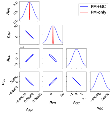
Figure 2: Constraints on the beyond vacuum-GR parameters $\{A_{\mathrm{PM}},n_{\mathrm{PM}},A_{\mathrm{GC}},n_{\mathrm{GC}}\}$ of an EMRI signal with only a significant PM effect, analyzed by PM-only (red) and PM+GC (blue) templates. All contours are 1-sigma.

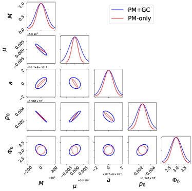
Figure 3: Constraints on the vacuum-GR parameters $\{M,\mu,a,p_{0},\Phi_{0}\}$ of an EMRI signal with only a signifcant PM effect, analyzed by PM-only (red) and PM+GC (blue) templates. All contours are 1-sigma.

Case i@ examples.

We first examine the joint analysis of the PM and GC effects in a signal that only has a significant PM effect. This represents the more general case of searching for modified-gravity effects in environment-rich EMRIs. The PM parameters of the signal are set as $(A_{\mathrm{PM}},n_{\mathrm{PM}})=(10^{-5},8)$, based on estimates in Kocsis et al. (2011), while the (unmeasurable) GC parameters are set as $(A_{\mathrm{GC}},n_{\mathrm{GC}})=(10^{-12},4)$. For a single-effect analysis (fixing the GC parameters to the signal values), the correlations between the vacuum-GR and PM parameter sets are $\lesssim 0.5$, consistent with the values reported in Speri et al. (2023). In the joint analysis, correlations of $\gtrsim 0.9$ are introduced between the PM and GC parameter sets. This leads to a degradation of the inference precision for $A_{\mathrm{PM}},n_{\mathrm{PM}}$ by an order of magnitude, making them effectively unmeasurable (see Fig. 2), as well as for the vacuum-GR parameters by a factor of $\lesssim 2$ (Fig. 3).

The strong correlations are driven by the high degree of similarity between the PM and GC effects as described in (8). Restoring the factor $(1-\sqrt{p_{\mathrm{in}}/p})^{m}$ to the PM effect (and adding $m=-12$ to the parameter set) thus reduces the correlations, with the inference degradation now by a factor of $\lesssim 2$ for all parameters in the joint analysis.

Case ii@ examples.

We now examine the analysis of the vacuum-GR parameters in a signal that has a significant PM effect. As in the Case I examples, the PM parameters are set as $(A_{\mathrm{PM}},n_{\mathrm{PM}})=(10^{-5},8)$. Using the leading-order bias estimate (7) with $\boldsymbol{\varphi}_{s}=(10^{-5},8)$ and $\boldsymbol{\varphi}_{0}=(0,0)$, we find that the bias-to-precision ratio $|\Delta\theta_{i}|/(\Sigma_{ii})^{1/2}$ for all vacuum-GR parameters $\boldsymbol{\psi}$ is $>10$, i.e., their inference incurs significant biases. These biases explicitly scale with the covariances $\Sigma_{\boldsymbol{\psi}\boldsymbol{\phi}}$, since See Supplemental Material at [URL will be inserted by publisher] for “A linear-signal-regime estimate of the inference bias incurred in nested models”. ; Boyd and Vandenberghe (2004)

$$(\Gamma_{\boldsymbol{\psi}\boldsymbol{\psi}})^{-1}\Gamma_{\boldsymbol{\psi}\boldsymbol{\varphi}}=-\Sigma_{\boldsymbol{\psi}\boldsymbol{\varphi}}(\Sigma_{\boldsymbol{\varphi}\boldsymbol{\varphi}})^{-1}.$$ (9)

In addition to biases, multimodal posteriors will generally arise due to the nonlinear embedding of the signal manifold $\mathcal{S}$ in the data space Chua (2020), as depicted in Fig. 1. Beyond its inconveniencing of posterior sampling in GW inference, this phenomenon severely hinders the prospects of searching for EMRIs in LISA data Chua and Cutler (2022). In the context of beyond vacuum-GR inference, the degree of multimodality is likely to increase with the number of effects under consideration (both modeled and unmodeled); e.g., with the PM and GC effects in the signal but only one or neither of them in the templates. However, the linear-signal framework we adopt here describes only local correlations, and is thus unsuitable for a study of multimodality.

Consequences for the ppE formalism.

We now highlight how our analysis extends to other current themes in the modeling of LISA EMRIs. The ppE formalism described earlier is a popular framework for introducing modified gravity effects at the level of the waveform. When constraining multiple such effects simultaneously, the modified template would presumably take the form:

$$\tilde{h}(f)=\tilde{h}_{\mathrm{GR}}(f)\left(1+\Sigma_{k}A_{k}u^{a_{k}}\right)\exp[i\left(\Sigma_{k}B_{k}u^{b_{k}}\right)],$$ (10)

where $\tilde{h}_{\mathrm{GR}}(f)$ is the vacuum-GR waveform with $u\equiv f\pi(M\mu)^{3/5}/(M+\mu)^{1/5}$; $A_{k}$ and $B_{k}$ dictate the amplitude and phase strength of the $k$-th effect, respectively; and $a_{k}$ and $b_{k}$ are related to the PN order of the effect. In combination with our earlier calculation See Supplemental Material at [URL will be inserted by publisher] for “Correlations between parameters of a beyond vacuum-GR EMRI do not vanish if an effect is absent”. , it is straightforward to show that See Supplemental Material at [URL will be inserted by publisher] for “Consequences for the ppE formalism”. the ppE formalism is generically susceptible to the same problems highlighted above for Case i@: if an effect is modeled in the ppE template but not actually present in the signal, its non-amplitude parameters become effectively unmeasurable, and their non-vanishing correlations with all other parameters in the analysis can severely hinder joint inference.

Consequences for the EMRI secondary spin.

To meet the science requirements of LISA, the long-term evolution of vacuum-GR EMRIs must be described accurately up to first post-adiabatic (1PA) order Hinderer and Flanagan (2008); Pound and Wardell (2021) when expanding in the small mass ratio $\epsilon\equiv\mu/M$, i.e., models must include all $\mathcal{O}(\epsilon)$ corrections to the leading-order adiabatic (0PA) evolution Hughes et al. (2021); Isoyama et al. (2022). The spin $\chi$ of the secondary mass becomes relevant at this order Mathews et al. (2022). For a circular and equatorial EMRI, the energy flux can be written as Burke et al. (2023)

$$\dot{E}=\dot{E}_{\mathrm{0PA}}(\boldsymbol{\psi}_{0})+\epsilon\dot{E}_{\mathrm{SF}}(\boldsymbol{\psi}_{0})+\epsilon\dot{E}_{\chi}(\boldsymbol{\psi}_{0},\chi)+\mathcal{O}(\epsilon^{2}),$$ (11)

where $\boldsymbol{\psi}_{0}$ is the 0PA vacuum-GR parameter set, $\dot{E}_{\mathrm{0PA}}$ is the adiabatic flux, and the 1PA term has been split into two: $\dot{E}_{\chi}$, which contains all contributions from $\chi$, and $\dot{E}_{\mathrm{SF}}$, which contains all other self-force corrections.

Eq. (11) can be cast in the form of Eq. (1), with $\dot{E}_{\mathrm{GR}}\equiv\dot{E}_{\mathrm{0PA}}+\epsilon\dot{E}_{\mathrm{SF}}$, $\mathcal{F}\equiv\dot{E}_{\chi}/(\dot{E}_{\mathrm{0PA}}+\epsilon\dot{E}_{\mathrm{SF}})$, and $(\boldsymbol{\psi},A,\boldsymbol{\phi})\equiv(\boldsymbol{\psi}_{0},\epsilon,\chi)$. Since $\epsilon\ll 1$ for an EMRI, $\chi$ is generally poorly constrained, if at all measurable (in the same way that $(\Sigma_{\boldsymbol{\phi}\boldsymbol{\phi}})^{1/2}\to\infty$ as $A\to 0$). This was observed by Burke et al. Burke et al. (2023), who found that $\chi$ in a circular Schwarzschild EMRI is significantly better measured when $\epsilon=10^{-4}$ than when $\epsilon=10^{-5}$. Previous studies also drew similar conclusions on the overall measurability of $\chi$ Piovano et al. (2021); Huerta and Gair (2011). At the same time, the correlations between $\chi$ and $\boldsymbol{\psi}_{0}$ do not vanish in general, which would degrade the inference precision of the latter relative to using a template model with no secondary spin (this was not examined in Burke et al. (2023)).

Directions forward.

Strong correlations among beyond vacuum-GR effects in EMRIs typically arise due to simplistic models of those effects. The most direct way forward is thus to improve the modeling end, e.g., by adding detail to the description of the PM effect as shown earlier. Cole et al. Cole et al. (2022) also recently demonstrated the joint Bayesian inference of three beyond vacuum-GR effects, albeit with some simplistic assumptions on the analysis. Note that improved modeling of such effects still does not guarantee their decoupling in inference, simply because many of them are inherently perturbative (small-amplitude) and secular (long-timescale). In contrast, if an effect manifests as a transient resonance Hinderer and Flanagan (2008); Berry et al. (2016); Gupta et al. (2022); Mukherjee and Tripathy (2020), for example, it is likely to be more distinguishable from secular-type effects.

If more detailed models are not available (be it due to modeling difficulty or the actual simplicity of the effect), there are limited solutions on the analysis end. In similar spirit to “agnostic” parametric tests of GR, one could construct a beyond vacuum-GR model with only a single set of effect parameters, to perform a null test of the vacuum-GR hypothesis and to measure any potential deviation (e.g., the ppE formalism, or parametrised tests of GR used in ground-based observing Li et al. (2012); Saleem et al. (2022); Krishnendu and Ohme (2021)). The functional dependence of the model on these parameters would attempt to generically describe most beyond vacuum-GR deviations (e.g., a power law, or perturbations to PN coefficients). In the context of the LISA global fit strategy Cornish and Crowder (2005); Vallisneri (2009); Babak et al. (2010), this scheme would be more practically viable than the additive modeling of multiple effects; however, it would be subject to the usual pitfalls when introducing arbitrary degrees of freedom into a physical model Chua and Vallisneri (2020). For example, any such model will be far more sensitive to some effects than others, potentially leading to severe selection bias. Furthermore, if multiple effects are truly present in the signal, the approach hinges strongly on our ability to find and interpret the multiple posterior modes.

An alternative strategy could be to rely on population-level studies. A catalog of detected sources might provide combined evidence for the presence of global effects (e.g., the time-varying gravitational constant) over local ones (e.g., accretion disks or boson stars Macedo et al. (2013a, b)), thus decoupling them within a hierarchical Bayesian model (e.g., Moore and Gerosa (2021)). Such approaches and others will be needed to circumvent the problems caused by effect correlations and to unlock the full potential of EMRIs as high-precision probes of modified gravity and astrophysical environments.

.1 Correlations between parameters of a beyond vacuum-GR EMRI do not vanish if an effect is absent

As noted in the Letter, we can write the partial derivatives of the waveform template $h(\dot{E},\dot{L})$ as

$$\frac{\partial{h(\dot{E},\dot{L})}}{\partial\theta_{i}}=\frac{\partial h(\dot{E},\dot{L})}{\partial\dot{E}}\frac{\partial\dot{E}}{\partial\theta_{i}}+\frac{\partial h(\dot{E},\dot{L})}{\partial\dot{L}}\frac{\partial\dot{L}}{\partial\theta_{i}},$$ (12)

where the first partial in each term is a vector by vector derivative and the second partial is a vector by scalar derivative. The FIM elements are thus

$$\Gamma_{ij}(\boldsymbol{\theta})=\left.\left<\frac{\partial h}{\partial\dot{E}}\frac{\partial\dot{E}}{\partial\theta_{i}}+\frac{\partial h}{\partial\dot{L}}\frac{\partial\dot{L}}{\partial\theta_{i}}\right|\frac{\partial h}{\partial\dot{E}}\frac{\partial\dot{E}}{\partial\theta_{j}}+\frac{\partial h}{\partial\dot{L}}\frac{\partial\dot{L}}{\partial\theta_{j}}\right>.$$ (13)

For two effects indexed $i=1,2$, the fluxes in a generic beyond vacuum-GR EMRI model take the form

$$\dot{E} =\dot{E}_{\mathrm{GR}}(\boldsymbol{\psi})\left(1+\sum_{k=1}^{2}A_{k}(\alpha_{k})\mathcal{F}_{k}(\boldsymbol{\psi},\boldsymbol{\phi_{k}})\right),$$ (14)

$$\dot{L} =\dot{L}_{\mathrm{GR}}(\boldsymbol{\psi})\left(1+\sum_{k=1}^{2}B_{k}(\alpha_{k})\mathcal{G}_{i}(\boldsymbol{\psi},\boldsymbol{\phi_{k}})\right).$$ (15)

We now show that all correlation coefficients $\rho_{ij}\equiv\Sigma_{ij}/(\Sigma_{ii}\Sigma_{jj})^{1/2}$ are $\mathcal{O}(1)$ as one of the effects vanishes ($\alpha_{2}\to 0$, without loss of generality). For $\alpha_{2}$ and each component of $\boldsymbol{\phi}_{2}$, we have for all other parameters $\theta$:

$$\Gamma_{\theta\theta} =\langle\mathcal{O}(1)|\mathcal{O}(1)\rangle=\mathcal{O}(1)$$ (16)

$$\Gamma_{\theta\alpha_{2}} =\left.\left<\mathcal{O}(1)\right|A_{2}^{\prime}(\alpha_{2})\times\mathcal{O}(1)+B_{2}^{\prime}(\alpha_{2})\times\mathcal{O}(1)\right>=\epsilon_{2}^{\prime}\times\mathcal{O}(1)$$ (17)

$$\Gamma_{\theta\phi_{2}} =\left.\left<\mathcal{O}(1)\right|A_{2}(\alpha_{2})\times\mathcal{O}(1)+B_{2}(\alpha_{2})\times\mathcal{O}(1)\right>=\epsilon_{2}\times\mathcal{O}(1)$$ (18)

$$\Gamma_{\alpha_{2}\alpha_{2}} =\left.\left<A_{2}^{\prime}(\alpha_{2})\times\mathcal{O}(1)+B_{2}^{\prime}(\alpha_{2})\times\mathcal{O}(1)\right|A_{2}^{\prime}(\alpha_{2})\times\mathcal{O}(1)+B_{2}^{\prime}(\alpha_{2})\times\mathcal{O}(1)\right>=(\epsilon_{2}^{\prime})^{2}\times\mathcal{O}(1)$$ (19)

$$\Gamma_{\alpha_{2}\phi_{2}} =\left.\left<A_{2}^{\prime}(\alpha_{2})\times\mathcal{O}(1)+B_{2}^{\prime}(\alpha_{2})\times\mathcal{O}(1)\right|A_{2}(\alpha_{2})\times\mathcal{O}(1)+B_{2}(\alpha_{2})\times\mathcal{O}(1)\right>=\epsilon_{2}^{\prime}\epsilon_{2}\times\mathcal{O}(1)$$ (20)

$$\Gamma_{\phi_{2}\phi_{2}} =\left.\left<A_{2}(\alpha_{2})\times\mathcal{O}(1)+B_{2}(\alpha_{2})\times\mathcal{O}(1)\right|A_{2}(\alpha_{2})\times\mathcal{O}(1)+B_{2}(\alpha_{2})\times\mathcal{O}(1)\right>=\epsilon_{2}^{2}\times\mathcal{O}(1),$$ (21)

as $\alpha_{2}\to 0$, where

$$\epsilon_{2}^{\prime}\equiv\begin{cases}A_{2}^{\prime}&\text{if }B_{2}^{\prime}=\mathcal{O}(A_{2}^{\prime})\\ B_{2}^{\prime}&\text{if }A_{2}^{\prime}=o(B_{2}^{\prime})\end{cases},$$ (22)

$$\epsilon_{2}\equiv\begin{cases}A_{2}&\text{if }B_{2}=\mathcal{O}(A_{2})\\ B_{2}&\text{if }A_{2}=o(B_{2})\end{cases},$$ (23)

with $(A_{2}^{\prime},B_{2}^{\prime})$ denoting $\partial_{\alpha_{2}}(A_{2},B_{2})$, $x=\mathcal{O}(y)$ denoting $\mathrm{lim\,sup}_{\alpha_{2}\to 0}(|x|/|y|)<\infty$, and $x=o(y)$ denoting $\mathrm{lim}_{\alpha_{2}\to 0}(x/y)=0$. In short, $\epsilon_{2}^{\prime}$ factors out of every row and column of $\Gamma$ that involves $\alpha_{2}$, while $\epsilon_{2}$ factors out of every row and column that involves a component of $\boldsymbol{\phi}_{2}$.

Then we observe that

$$\Sigma_{ij}=\left(\Gamma^{-1}\right)_{ij}=\frac{1}{|\Gamma|}C_{ij}\implies\rho_{ij}=\frac{C_{ij}}{\sqrt{C_{ii}C_{jj}}},$$ (24)

where $C$ is the cofactor matrix of $\Gamma$ (since $\Gamma$ is symmetric). From the above scaling relations, we have

$$C_{\theta\theta} =(\epsilon_{2}^{\prime})^{2}\epsilon_{2}^{2d}\times\mathcal{O}(1)$$ (25)

$$C_{\theta\alpha_{2}} =\epsilon_{2}^{\prime}\epsilon_{2}^{2d}\times\mathcal{O}(1)$$ (26)

$$C_{\theta\phi_{2}} =(\epsilon_{2}^{\prime})^{2}\epsilon_{2}^{2d-1}\times\mathcal{O}(1)$$ (27)

$$C_{\alpha_{2}\alpha_{2}} =\epsilon_{2}^{2d}\times\mathcal{O}(1)$$ (28)

$$C_{\alpha_{2}\phi_{2}} =\epsilon_{2}^{\prime}\epsilon_{2}^{2d-1}\times\mathcal{O}(1)$$ (29)

$$C_{\phi_{2}\phi_{2}} =(\epsilon_{2}^{\prime})^{2}\epsilon_{2}^{2d-2}\times\mathcal{O}(1),$$ (30)

where $d$ is the dimensionality of $\boldsymbol{\phi}_{2}$. It follows trivially from Eq. (24) that $\rho_{ij}=\mathcal{O}(1)$ for all $i,j$.

.2 A linear-signal-regime estimate of the inference bias incurred in nested models

We consider the subcase of Case ii@ where $\mathcal{T}\subset\mathcal{S}$. The signal model is $h_{\mathcal{S}}(\boldsymbol{\psi},\boldsymbol{\varphi})$ and the template model is $h_{\mathcal{T}}(\boldsymbol{\psi})\equiv h_{\mathcal{S}}(\boldsymbol{\psi},\boldsymbol{\varphi}=\boldsymbol{\varphi}_{0})$, where $\boldsymbol{\varphi}_{0}$ is some value of $\boldsymbol{\varphi}$ for which the effect described by $\boldsymbol{\varphi}$ vanishes. The signal is $s=h_{\mathcal{S}}(\boldsymbol{\psi}_{s},\boldsymbol{\varphi}_{s})\in\mathcal{S}$. Analysing it with the template model yields a maximum-likelihood template $h_{\mathcal{T}}(\boldsymbol{\psi}_{\mathrm{ML}})=h_{\mathcal{S}}(\boldsymbol{\psi}_{\mathrm{ML}},\boldsymbol{\varphi}_{0})$. By definition, $\boldsymbol{\psi}_{\mathrm{ML}}$ satisfies

$$\langle\partial_{(\boldsymbol{\psi},\boldsymbol{\varphi})}h_{\mathcal{S}}(\boldsymbol{\psi},\boldsymbol{\varphi}=\boldsymbol{\varphi}_{0})|_{\boldsymbol{\psi}=\boldsymbol{\psi}_{\mathrm{ML}}}|s-h_{\mathcal{S}}(\boldsymbol{\psi}_{\mathrm{ML}},\boldsymbol{\varphi}_{0})\rangle=0.$$ (31)

Note that the derivative vector reduces to $((\partial_{\boldsymbol{\psi}}h_{\mathcal{T}})(\boldsymbol{\psi}_{\mathrm{ML}}),0)$, and is not generally equivalent to $(\partial_{(\boldsymbol{\psi},\boldsymbol{\varphi})}h_{\mathcal{S}})(\boldsymbol{\psi}_{\mathrm{ML}},\boldsymbol{\varphi}_{0})$, since the derivative of an effect amplitude parameter does not generally vanish at $\boldsymbol{\varphi}_{0}$.

One may nonetheless proceed with the Cutler–Vallisneri derivation Cutler and Vallisneri (2007) on the ambient manifold $\mathcal{S}$ rather than $\mathcal{T}$. Define the inference bias in $\boldsymbol{\psi}$ as $\Delta\boldsymbol{\psi}\equiv\boldsymbol{\psi}_{\mathrm{ML}}-\boldsymbol{\psi}_{s}$. Expanding $h_{\mathcal{S}}(\boldsymbol{\psi}_{s},\boldsymbol{\varphi}_{0})$ about $(\boldsymbol{\psi}_{\mathrm{ML}},\boldsymbol{\varphi}_{0})$ to first order in $(\Delta\boldsymbol{\psi},0)$, and substituting into the maximum-likelihood constraint (31), we find

$$\langle\partial_{(\boldsymbol{\psi},\boldsymbol{\varphi})}h_{\mathcal{S}}(\boldsymbol{\psi},\boldsymbol{\varphi}=\boldsymbol{\varphi}_{0})|_{\boldsymbol{\psi}=\boldsymbol{\psi}_{\mathrm{ML}}}|s-h_{\mathcal{S}}(\boldsymbol{\psi}_{s},\boldsymbol{\varphi}_{0})\rangle=\langle\partial_{(\boldsymbol{\psi},\boldsymbol{\varphi})}h_{\mathcal{S}}(\boldsymbol{\psi},\boldsymbol{\varphi}=\boldsymbol{\varphi}_{0})|_{\boldsymbol{\psi}=\boldsymbol{\psi}_{\mathrm{ML}}}|(\partial_{(\boldsymbol{\psi},\boldsymbol{\varphi})}h_{\mathcal{S}})(\boldsymbol{\psi}_{\mathrm{ML}},\boldsymbol{\varphi}_{0})\rangle\cdot(\Delta\boldsymbol{\psi},0)$$

$$\Rightarrow\begin{bmatrix}\langle\partial_{\boldsymbol{\psi}}h_{\mathcal{S}}(\boldsymbol{\psi},\boldsymbol{\varphi}=\boldsymbol{\varphi}_{0})|_{\boldsymbol{\psi}=\boldsymbol{\psi}_{\mathrm{ML}}}|s-h_{\mathcal{S}}(\boldsymbol{\psi}_{s},\boldsymbol{\varphi}_{0})\rangle\\ 0\end{bmatrix}=\begin{bmatrix}\Gamma_{\boldsymbol{\psi}\boldsymbol{\psi}}(\boldsymbol{\psi}_{\mathrm{ML}},\boldsymbol{\varphi}_{0})&\Gamma_{\boldsymbol{\psi}\boldsymbol{\varphi}}(\boldsymbol{\psi}_{\mathrm{ML}},\boldsymbol{\varphi}_{0})\\ 0&0\end{bmatrix}\cdot\begin{bmatrix}\Delta\boldsymbol{\psi}\\ 0\end{bmatrix}.$$ (32)

Once again, note that the outer product on the right side is not the FIM on $\mathcal{S}$, and in particular is non-invertible since it has zero rows. However, as both sides of (32) have the same zero rows (corresponding to $\boldsymbol{\varphi}$), it simplifies to

$$\langle(\partial_{\boldsymbol{\psi}}h_{\mathcal{T}})(\boldsymbol{\psi}_{\mathrm{ML}})|s-h_{\mathcal{T}}(\boldsymbol{\psi}_{s})\rangle=\Gamma_{\boldsymbol{\psi}\boldsymbol{\psi}}(\boldsymbol{\psi}_{\mathrm{ML}})\cdot\Delta\boldsymbol{\psi},$$ (33)

which is the Cutler–Vallisneri equation on $\mathcal{T}$, as expected.

Note that the original application of Eq. (33) is to estimate the signal parameters given the maximum-likelihood estimate $\boldsymbol{\psi}_{\mathrm{ML}}$ from an approximate model $h_{\mathcal{T}}$, and thus relies on approximating the waveform difference on the left side at $\boldsymbol{\psi}_{\mathrm{ML}}$ instead of $\boldsymbol{\psi}_{s}$. This approach breaks down here since $\mathcal{T}\subset\mathcal{S}$, but is not actually needed since we are assuming that $\boldsymbol{\psi}_{s}$ is known instead (and wish to estimate the bias $\Delta\boldsymbol{\psi}$). We simply use the fact that to leading order, both the waveform derivatives and the FIM are invariant as $(\boldsymbol{\psi}_{\mathrm{ML}},\boldsymbol{\varphi}_{0})\to(\boldsymbol{\psi}_{s},\boldsymbol{\varphi}_{0})$ (the whole Cutler–Vallisneri approach is invalid anyway if one is not in the linear-signal regime).

Although not immediately evident in Eq. (33), the correlations between $\boldsymbol{\psi}$ and $\boldsymbol{\varphi}$ still affect the bias, but through the signal $s$ rather than the FIM on $\mathcal{T}$ (which does not depend on $\boldsymbol{\varphi}$ in the first place). We perform further expansions of $s=h_{\mathcal{S}}(\boldsymbol{\psi}_{s},\boldsymbol{\varphi}_{s})$ and $h_{\mathcal{S}}(\boldsymbol{\psi}_{s},\boldsymbol{\varphi}_{0})$ about $(\boldsymbol{\psi}_{\mathrm{ML}},\boldsymbol{\varphi}_{0})$, and a substitution into Eq. (32) gives

$$\begin{bmatrix}\Gamma_{\boldsymbol{\psi}\boldsymbol{\psi}}&\Gamma_{\boldsymbol{\psi}\boldsymbol{\varphi}}\\ 0&0\end{bmatrix}\cdot\begin{bmatrix}0\\ \boldsymbol{\varphi}_{s}-\boldsymbol{\varphi}_{0}\end{bmatrix}=\begin{bmatrix}\Gamma_{\boldsymbol{\psi}\boldsymbol{\psi}}&\Gamma_{\boldsymbol{\psi}\boldsymbol{\varphi}}\\ 0&0\end{bmatrix}\cdot\begin{bmatrix}\Delta\boldsymbol{\psi}\\ 0\end{bmatrix},$$ (34)

where $\Gamma_{\boldsymbol{\psi}\boldsymbol{\psi}}$ and $\Gamma_{\boldsymbol{\psi}\boldsymbol{\varphi}}$ are submatrices of the “FIM” on $\mathcal{S}$, evaluated at $(\boldsymbol{\psi}_{s},\boldsymbol{\varphi}_{0})$ instead of $(\boldsymbol{\psi}_{\mathrm{ML}},\boldsymbol{\varphi}_{0})$. Thus

$$\Delta\boldsymbol{\psi}=(\Gamma_{\boldsymbol{\psi}\boldsymbol{\psi}})^{-1}\Gamma_{\boldsymbol{\psi}\boldsymbol{\varphi}}\cdot(\boldsymbol{\varphi}_{s}-\boldsymbol{\varphi}_{0}),$$ (35)

which describes to leading order the bias incurred when performing inference with a template model that is a nested submodel of the signal model. Via the matrix inversion lemma Boyd and Vandenberghe (2004), we may also write the matrix $(\Gamma_{\boldsymbol{\psi}\boldsymbol{\psi}})^{-1}\Gamma_{\boldsymbol{\psi}\boldsymbol{\varphi}}$ in terms of submatrices of the inverse FIM $\Sigma=\Gamma^{-1}$:

$$(\Gamma_{\boldsymbol{\psi}\boldsymbol{\psi}})^{-1}\Gamma_{\boldsymbol{\psi}\boldsymbol{\varphi}}=-\Sigma_{\boldsymbol{\psi}\boldsymbol{\varphi}}(\Sigma_{\boldsymbol{\varphi}\boldsymbol{\varphi}})^{-1},$$ (36)

which shows the explicit relationship between the parameter biases $\Delta\boldsymbol{\psi}$ and the parameter covariances $\Sigma_{\boldsymbol{\psi}\boldsymbol{\phi}}$.

.3 Consequences for the ppE formalism

In the ppE formalism Yunes and Pretorius (2009), the modification of a frequency-domain inspiral waveform by two beyond vacuum-GR effects is (by natural extension) written as

$$\tilde{h}(f)=\tilde{h}_{\mathrm{GR}}(f)\left(1+\Sigma_{k}^{2}A_{k}u^{a_{k}}\right)\exp[i\left(\Sigma_{k}^{2}B_{k}u^{b_{k}}\right)],$$ (37)

where $\tilde{h}_{\mathrm{GR}}(f)$ is the vacuum-GR waveform and $\{A_{k},a_{k},B_{k},b_{k}\}$ is the parameter set for effect $k$. We focus on the vanishing of the second effect in the signal, such that the corresponding amplitudes $A_{2},B_{2}\to 0$. The partial derivatives of $\tilde{h}(f)$ with respect to $(a_{2},b_{2})$ also vanish proportionally to $(A_{2},B_{2})$:

$$\frac{\partial\tilde{h}(f)}{\partial a_{2}}=A_{2}\times u^{a_{2}}\mathcal{H},$$ (38)

$$\frac{\partial\tilde{h}(f)}{\partial b_{2}}=B_{2}\times iu^{b_{2}}(1+A_{1}u^{a_{1}}+A_{2}u^{a_{2}})\mathcal{H},$$ (39)

where

$$\mathcal{H}=\tilde{h}_{\mathrm{GR}}(f)\ln{(u)}\exp[i\left(B_{1}u^{b_{1}}+B_{2}u^{b_{2}}\right)].$$ (40)

Since the Fourier transform commutes with partial derivatives ($\tilde{(\partial h)}=\partial\tilde{h}$) in the standard matched-filtering inner product Barack and Cutler (2004) (weighted by detector noise with power spectral density $S_{n}(f)$), we have

$$\Gamma_{ij}=\left.\left<\frac{\partial h}{\partial\theta_{i}}\right|\frac{\partial h}{\partial\theta_{j}}\right>=2\int_{0}^{\infty}\frac{(\partial_{i}\tilde{h})^{\dagger}\partial_{j}\tilde{h}+(\partial_{j}\tilde{h})^{\dagger}\partial_{i}\tilde{h}}{S_{n}(f)}\,df.$$ (41)

It is then straightforward to see that $A_{2}$ factors out of every row and column of the FIM that involves $a_{2}$, while $B_{2}$ factors out of every row and column that involves $b_{2}$. Thus, similar to the argument in the first section of the Supplemental Material, the correlations between $a_{2}$ or $b_{2}$ and all other parameters are $\mathcal{O}(1)$ as effect 2 vanishes. At the same time, the precisions to which $a_{2},b_{2}$ can be measured blow up in the same limit, and so the inference of other parameters is generally worsened as well.

References

- Amaro-Seoane et al. (2015) P. Amaro-Seoane, J. R. Gair, A. Pound, S. A. Hughes, and C. F. Sopuerta, Journal of Physics: Conference Series 610, 012002 (2015).
- Barack and Cutler (2004) L. Barack and C. Cutler, Physical Review D 69 (2004), 10.1103/physrevd.69.082005.
- Seoane et al. (2013) P. A. Seoane, et. al., and T. eLISA Consortium, “The gravitational universe,” (2013), arXiv:1305.5720 [astro-ph.CO] .
- Seoane et al. (2017) P. A. Seoane, et. al., and T. eLISA Consortium, “Laser interferometer space antenna,” (2017).
- Seoane et al. (2012a) P. A. Seoane, et. al., and T. eLISA Consortium, Classical and Quantum Gravity 29, 124016 (2012a).
- Seoane et al. (2012b) P. A. Seoane, et. al., and T. eLISA Consortium, “elisa: Astrophysics and cosmology in the millihertz regime,” (2012b), arXiv:1201.3621 [astro-ph.CO] .
- Amaro-Seoane et al. (2007) P. Amaro-Seoane, J. R. Gair, M. Freitag, M. C. Miller, I. Mandel, C. J. Cutler, and S. Babak, Classical and Quantum Gravity 24, R113 (2007).
- Amaro-Seoane (2018) P. Amaro-Seoane, Living Reviews in Relativity 21 (2018), 10.1007/s41114-018-0013-8.
- Gair et al. (2013) J. R. Gair, M. Vallisneri, S. L. Larson, and J. G. Baker, Living Reviews in Relativity 16 (2013), 10.12942/lrr-2013-7.
- Babak et al. (2017) S. Babak, J. Gair, A. Sesana, E. Barausse, C. F. Sopuerta, C. P. Berry, E. Berti, P. Amaro-Seoane, A. Petiteau, and A. Klein, Physical Review D 95 (2017), 10.1103/physrevd.95.103012.
- Berry et al. (2019) C. P. L. Berry, S. A. Hughes, C. F. Sopuerta, A. J. K. Chua, A. Heffernan, K. Holley-Bockelmann, D. P. Mihaylov, M. C. Miller, and A. Sesana, (2019), arXiv:1903.03686 [astro-ph.HE] .
- Chamberlain and Yunes (2017) K. Chamberlain and N. Yunes, Physical Review D 96 (2017), 10.1103/physrevd.96.084039.
- Wang et al. (2022) Z. Wang, J. Zhao, Z. An, L. Shao, and Z. Cao, Physics Letters B 834, 137416 (2022).
- Barausse et al. (2016) E. Barausse, N. Yunes, and K. Chamberlain, Physical Review Letters 116 (2016), 10.1103/physrevlett.116.241104.
- Yunes et al. (2010) N. Yunes, F. Pretorius, and D. Spergel, Physical Review D 81 (2010), 10.1103/physrevd.81.064018.
- Barbieri et al. (2023) R. Barbieri, S. Savastano, L. Speri, A. Antonelli, L. Sberna, O. Burke, J. Gair, and N. Tamanini, Physical Review D 107 (2023), 10.1103/physrevd.107.064073.
- Cardoso et al. (2011) V. Cardoso, S. Chakrabarti, P. Pani, E. Berti, and L. Gualtieri, Physical Review Letters 107 (2011), 10.1103/physrevlett.107.241101.
- Barsanti et al. (2023) S. Barsanti, A. Maselli, T. P. Sotiriou, and L. Gualtieri, Physical Review Letters 131 (2023), 10.1103/physrevlett.131.051401.
- Yunes et al. (2012) N. Yunes, P. Pani, and V. Cardoso, Physical Review D 85 (2012), 10.1103/physrevd.85.102003.
- Barausse et al. (2014) E. Barausse, V. Cardoso, and P. Pani, Physical Review D 89 (2014), 10.1103/physrevd.89.104059.
- Kocsis et al. (2011) B. Kocsis, N. Yunes, and A. Loeb, Physical Review D 84 (2011), 10.1103/physrevd.84.024032.
- Yunes et al. (2011) N. Yunes, B. Kocsis, A. Loeb, and Z. Haiman, Physical Review Letters 107 (2011), 10.1103/physrevlett.107.171103.
- Zwick et al. (2023) L. Zwick, P. R. Capelo, and L. Mayer, Monthly Notices of the Royal Astronomical Society 521, 4645 (2023).
- Rahman et al. (2023) M. Rahman, S. Kumar, and A. Bhattacharyya, (2023), arXiv:2306.14971 [gr-qc] .
- Speri et al. (2023) L. Speri, A. Antonelli, L. Sberna, S. Babak, E. Barausse, J. R. Gair, and M. L. Katz, Physical Review X 13 (2023), 10.1103/physrevx.13.021035.
- Pound and Wardell (2021) A. Pound and B. Wardell, in Handbook of Gravitational Wave Astronomy (Springer Singapore, 2021) pp. 1–119.
- Barack and Pound (2018) L. Barack and A. Pound, Reports on Progress in Physics 82, 016904 (2018).
- Teukolsky (1973) S. A. Teukolsky, ApJ 185, 635 (1973).
- Hinderer and Flanagan (2008) T. Hinderer and É . É. Flanagan, Physical Review D 78 (2008), 10.1103/physrevd.78.064028.
- Fujita and Shibata (2020) R. Fujita and M. Shibata, Physical Review D 102 (2020), 10.1103/physrevd.102.064005.
- Isoyama et al. (2022) S. Isoyama, R. Fujita, A. J. Chua, H. Nakano, A. Pound, and N. Sago, Physical Review Letters 128 (2022), 10.1103/physrevlett.128.231101.
- Hughes et al. (2021) S. A. Hughes, N. Warburton, G. Khanna, A. J. Chua, and M. L. Katz, Physical Review D 103 (2021), 10.1103/physrevd.103.104014.
- Carter (1968) B. Carter, Phys. Rev. 174, 1559 (1968).
- Sago et al. (2006) N. Sago, T. Tanaka, W. Hikida, K. Ganz, and H. Nakano, Progress of Theoretical Physics 115, 873–907 (2006).
- Blanchet (2006) L. Blanchet, Living Reviews in Relativity 9, 4 (2006).
- Will (2006) C. M. Will, Living Reviews in Relativity 9 (2006), 10.12942/lrr-2006-3.
- Brans and Dicke (1961) C. Brans and R. H. Dicke, Phys. Rev. 124, 925 (1961).
- Will (1993) C. M. Will, Theory and Experiment in Gravitational Physics (Cambridge University Press, 1993).
- Yunes and Pretorius (2009) N. Yunes and F. Pretorius, Physical Review D 80 (2009), 10.1103/physrevd.80.122003.
- Tahura and Yagi (2018) S. Tahura and K. Yagi, Physical Review D 98 (2018), 10.1103/physrevd.98.084042.
- Jordan and Schücking (1955) P. Jordan and E. Schücking, Schwerkraft und Weltall: Grundlagen der theoretischen Kosmologie, 2nd ed. (F. Vieweg Braunschweig, Braunschweig, 1955).
- Fierz (1956) M. Fierz, Helv. Phys. Acta 29, 128 (1956).
- Cutler and Vallisneri (2007) C. Cutler and M. Vallisneri, Physical Review D 76 (2007), 10.1103/physrevd.76.104018.
- Chua (2020) A. J. K. Chua, Stat. Comput. 30, 587 (2020), arXiv:1811.05494 [stat.CO] .
- Chua and Cutler (2022) A. J. Chua and C. J. Cutler, Physical Review D 106 (2022), 10.1103/physrevd.106.124046.
- Vallisneri (2008) M. Vallisneri, Physical Review D 77 (2008), 10.1103/physrevd.77.042001.
- (47) See Supplemental Material at [URL will be inserted by publisher] for “Correlations between parameters of a beyond vacuum-GR EMRI do not vanish if an effect is absent”., .
- (48) See Supplemental Material at [URL will be inserted by publisher] for “A linear-signal-regime estimate of the inference bias incurred in nested models”., .
- Chua et al. (2021) A. J. K. Chua, M. L. Katz, N. Warburton, and S. A. Hughes, Phys. Rev. Lett. 126, 051102 (2021), arXiv:2008.06071 [gr-qc] .
- Katz et al. (2021) M. L. Katz, A. J. K. Chua, L. Speri, N. Warburton, and S. A. Hughes, Phys. Rev. D 104, 064047 (2021).
- Chua et al. (2017) A. J. K. Chua, C. J. Moore, and J. R. Gair, Phys. Rev. D 96, 044005 (2017), arXiv:1705.04259 [gr-qc] .
- Cutler (1998) C. Cutler, Phys. Rev. D 57, 7089 (1998).
- Will (1993) C. M. Will, Theory and Experiment in Gravitational Physics (1993).
- Boyd and Vandenberghe (2004) S. Boyd and L. Vandenberghe, Convex Optimization, Berichte über verteilte messysteme No. pt. 1 (Cambridge University Press, 2004).
- (55) See Supplemental Material at [URL will be inserted by publisher] for “Consequences for the ppE formalism”., .
- Mathews et al. (2022) J. Mathews, A. Pound, and B. Wardell, Physical Review D 105 (2022), 10.1103/physrevd.105.084031.
- Burke et al. (2023) O. Burke, G. A. Piovano, N. Warburton, P. Lynch, L. Speri, C. Kavanagh, B. Wardell, A. Pound, L. Durkan, and J. Miller, (2023), arXiv:2310.08927 [gr-qc] .
- Piovano et al. (2021) G. A. Piovano, R. Brito, A. Maselli, and P. Pani, Phys. Rev. D 104, 124019 (2021), arXiv:2105.07083 [gr-qc] .
- Huerta and Gair (2011) E. A. Huerta and J. R. Gair, Physical Review D 84 (2011), 10.1103/physrevd.84.064023.
- Cole et al. (2022) P. S. Cole, G. Bertone, A. Coogan, D. Gaggero, T. Karydas, B. J. Kavanagh, T. F. M. Spieksma, and G. M. Tomaselli, (2022), arXiv:2211.01362 [gr-qc] .
- Berry et al. (2016) C. P. Berry, R. H. Cole, P. Cañizares, and J. R. Gair, Physical Review D 94 (2016), 10.1103/physrevd.94.124042.
- Gupta et al. (2022) P. Gupta, L. Speri, B. Bonga, A. J. K. Chua, and T. Tanaka, Phys. Rev. D 106, 104001 (2022), arXiv:2205.04808 [gr-qc] .
- Mukherjee and Tripathy (2020) S. Mukherjee and S. Tripathy, “Resonant orbits for a spinning particle in kerr spacetime,” (2020), arXiv:1905.04061 [gr-qc] .
- Li et al. (2012) T. G. F. Li, W. Del Pozzo, S. Vitale, C. Van Den Broeck, M. Agathos, J. Veitch, K. Grover, T. Sidery, R. Sturani, and A. Vecchio, Physical Review D 85 (2012), 10.1103/physrevd.85.082003.
- Saleem et al. (2022) M. Saleem, S. Datta, K. Arun, and B. Sathyaprakash, Physical Review D 105 (2022), 10.1103/physrevd.105.084062.
- Krishnendu and Ohme (2021) N. V. Krishnendu and F. Ohme, Universe 7, 497 (2021), arXiv:2201.05418 [gr-qc] .
- Cornish and Crowder (2005) N. J. Cornish and J. Crowder, Physical Review D 72 (2005), 10.1103/physrevd.72.043005.
- Vallisneri (2009) M. Vallisneri, Classical and Quantum Gravity 26, 094024 (2009).
- Babak et al. (2010) S. Babak, et al., the Mock LISA Data Challenge Task Force, M. Adams, et al., and the Challenge 3 participants, Classical and Quantum Gravity 27, 084009 (2010).
- Chua and Vallisneri (2020) A. J. K. Chua and M. Vallisneri, (2020), arXiv:2006.08918 [gr-qc] .
- Macedo et al. (2013a) C. F. B. Macedo, P. Pani, V. Cardoso, and L. C. B. Crispino, The Astrophysical Journal 774, 48 (2013a).
- Macedo et al. (2013b) C. F. B. Macedo, P. Pani, V. Cardoso, and L. C. B. Crispino, Physical Review D 88 (2013b), 10.1103/physrevd.88.064046.
- Moore and Gerosa (2021) C. J. Moore and D. Gerosa, Physical Review D 104 (2021), 10.1103/physrevd.104.083008.
Supplemental Material: Impact of Correlations on the Modeling and Inference of Beyond Vacuum-GR Effects in Extreme-Mass-Ratio Inspirals