Doubly Perturbed Task-Free Continual Learning

Abstract

Task-free online continual learning (TF-CL) is a challenging problem where the model incrementally learns tasks without explicit task information. Although training with entire data from the past, present as well as future is considered as the gold standard, naive approaches in TF-CL with the current samples may be conflicted with learning with samples in the future, leading to catastrophic forgetting and poor plasticity. Thus, a proactive consideration of an unseen future sample in TF-CL becomes imperative. Motivated by this intuition, we propose a novel TF-CL framework considering future samples and show that injecting adversarial perturbations on both input data and decision-making is effective. Then, we propose a novel method named Doubly Perturbed Continual Learning (DPCL) to efficiently implement these input and decision-making perturbations. Specifically, for input perturbation, we propose an approximate perturbation method that injects noise into the input data as well as the feature vector and then interpolates the two perturbed samples. For decision-making process perturbation, we devise multiple stochastic classifiers. We also investigate a memory management scheme and learning rate scheduling reflecting our proposed double perturbations. We demonstrate that our proposed method outperforms the state-of-the-art baseline methods by large margins on various TF-CL benchmarks.

Introduction

Continual learning (CL) addresses the challenge of effectively learning tasks when training data arrives sequentially. A notorious drawback of deep neural networks in a continual learning is catastrophic forgetting (McCloskey and Cohen 1989). As these networks learn new tasks, they often forget previously learned tasks, causing a decline in performance on those earlier tasks. If, on the other hand, we restrict the update in the network parameters to counteract the catastrophic forgetting, the learning capacity for newer tasks can be hindered. This dichotomy gives rise to what is known as the stability-plasticity dilemma (Carpenter and Grossberg 1987; Mermillod, Bugaiska, and Bonin 2013). The solutions to overcome this challenge fall into three main strategies: regularization-based methods (Kirkpatrick et al. 2017; Jung et al. 2020; Wang et al. 2021), rehearsal-based methods (Lopez-Paz and Ranzato 2017; Shin et al. 2017; Shmelkov, Schmid, and Alahari 2017; Chaudhry et al. 2018b, 2021), and architecture-based methods (Mallya and Lazebnik 2018; Serra et al. 2018).

In Task-Free online CL (TF-CL) (Aljundi, Kelchtermans, and Tuytelaars 2019), the model incrementally learns classes in an online manner agnostic to the task shift, which is considered more realistic and practical, but more challenging setup than offline CL (Koh et al. 2022; Zhang et al. 2022). The dominant approach to relieve forgetting in TF-CL is memory-based approaches  (Aljundi, Kelchtermans, and Tuytelaars 2019; Pourcel, Vu, and French 2022). They employ a small memory buffer to preserve a few past samples and replay them when training on a new task, but the restrictions on the available memory capacity highly degenerate performance on past tasks.

Rrecently, several works suggested evolving the memory by injecting perturbation on the memory samples to reduce the gap between true data distribution and the distribution in memory (Wang et al. 2022; Jin et al. 2021). Meanwhile, it has been successfully demonstrated that flattening sharpness of weight loss landscape can improve the performance on CL setups (Cha et al. 2020; Deng et al. 2021). However, most of the prior CL works primarily concentrated on past samples, often overlooking future samples. Note that many CL studies use “i.i.d. offline” as the oracle method for the best possible performance, which exhibits consistently low loss not only for past and present data, but also for future data. Therefore, incorporating unknown future samples in the CL model could be helpful in reducing forgetting and enhancing learning when training with real future samples.

In this work, we first demonstrate an upper bound for the TF-CL problem with unknown future samples, considering both adversarial input and weight perturbation, which has not been fully explained yet. Based on the observation, we propose a method, doubly perturbed continual learning (DPCL), addressing adversarial input perturbation with perturbed function interpolation and weight perturbation, specifically for classifier weights, through branched stochastic classifiers. Furthermore, we design a simple memory management strategy and adaptive learning rate scheduling induced by the perturbation. In experiments, our method significantly outperforms the existing rehearsal-based methods on various CL setups and benchmarks. Here is the summary of our contributions

• We propose an optimization framework for TF-CL and show that it has an upper bound which considers the adversarial input and weight perturbations.

• Our proposed method, DPCL, employs perturbed interpolation in function space and incorporates branching stochastic classifiers for both input and weight perturbations, with memory management and an adaptive learning rate derived from these perturbations.

• In experiments, the proposed method significantly improves the performance of baselines on various CL setups and benchmarks. We also have demonstrated the efficacy of adapting our method to existing algorithms, consistently yielding improvements in their performance.

Related Works

Continual learning (CL) seeks to retain prior knowledge while learning from sequential tasks that exhibit data distribution shifts. Most existing CL methods (Lopez-Paz and Ranzato 2017; Kirkpatrick et al. 2017; Chaudhry et al. 2018a; Zenke, Poole, and Ganguli 2017; Rolnick et al. 2019; Yoon et al. 2018; Mallya, Davis, and Lazebnik 2018; Hung et al. 2019) primarily focus on the offline setting, where the learner can repeatedly access task samples during training without time constraints and there are distinct task definitions that separate task sequences.

Task-Free online CL (TF-CL) (Aljundi, Kelchtermans, and Tuytelaars 2019; Chrysakis and Moens 2020; Jung et al. 2023; Pourcel, Vu, and French 2022; Ye and Bors 2022) addresses the more general scenario where the model incrementally learns classes in an online manner and the data distribution can change arbitrarily without explicit task information. The majority of existing TF-CL approaches fall under the rehearsal-based category (Aljundi, Kelchtermans, and Tuytelaars 2019; He et al. 2020; Wang et al. 2022). They involves storing a small number of data samples from the previous data stream and later replaying them alongside new mini-batch data. Therefore, we focus on rehearsal-based methods due to their simplicity and effectiveness.

Recently, GMED  (Jin et al. 2021) and DRO (Wang et al. 2022) proposed to edit memory samples by adversarial input perturbation, making it gradually harder to be memorized. Raghavan and Balaprakash (2021) have shown that the CL problem has an upper bound whose objective is to minimize with adversarial input perturbation due to uncertainty from future data. However, it didn’t fully consider the TF-CL setup. Meanwhile, Deng et al. (2021) demonstrated the effectiveness of applying adversarial weight perturbation on training and memory management for CL. To our best knowledge, it has not been investigated yet considering both input and weight perturbation simultaneously in TF-CL, and our work will propose a method that takes both into account.

Injecting input and weight perturbations into a standard training scheme is known to be effective for robustness and generalization by flattening the input and weight loss landscape. It is well known that flat input loss landscape is correlated to the robustness of performance of a network to input perturbations. In order to enhance robustness, adversarial training (AT) intentionally smooths out the input loss landscape by training on adversarially perturbed inputs. There are alternative approaches to flatten the loss landscape, through gradient regularization (Lyu, Huang, and Liang 2015; Ross and Doshi-Velez 2018), curvature regularization (Moosavi-Dezfooli et al. 2019), and local linearity regularization  (Qin et al. 2019). Meanwhile, multiple studies have demonstrated the correlation between the flat weight loss landscape and the standard generalization gap (Keskar et al. 2017; Neyshabur et al. 2017). Especially, adversarial weight perturbation (AWP) (Wu, Xia, and Wang 2020) effectively improved both standard and robust generalization by combining it with AT or other variants.

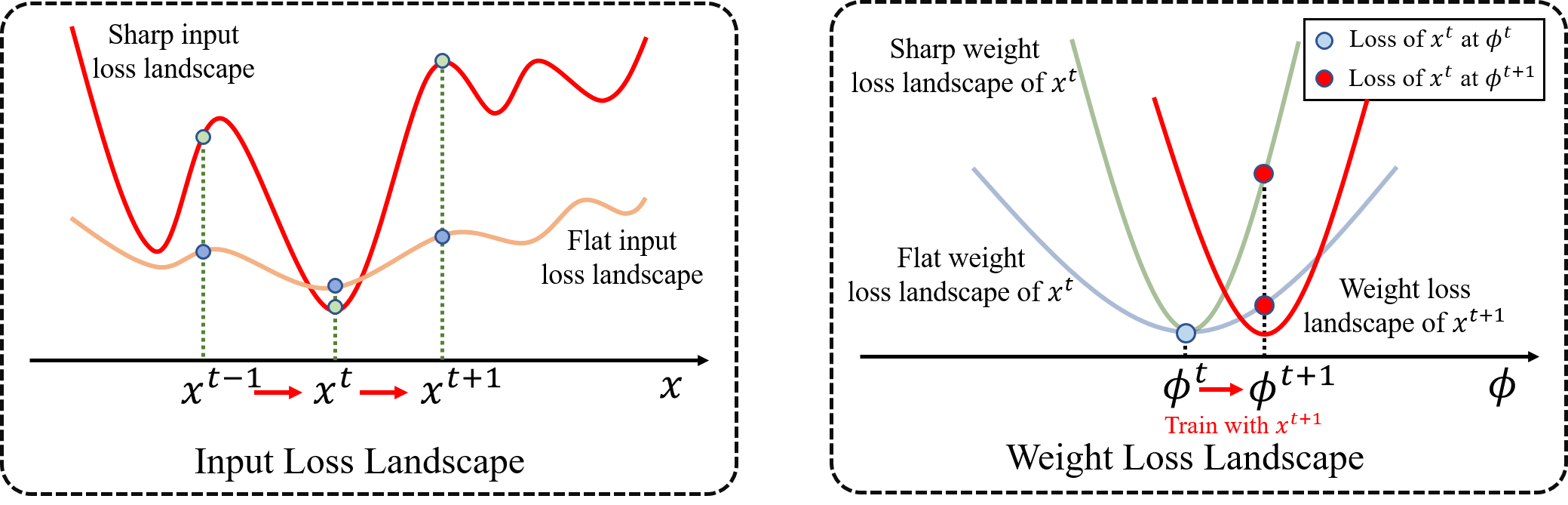
Figure 1: (Left) Input loss landscape of TF-CL when the weight $\theta^{t}$ has been determined for sample $x^{t}$. We desire $\ell(h(x;\theta^{t}),y)$ to be flat about $x^{t}$ so that the loss for $x^{\tau},\tau\in[1,\cdots,t-1,t+1]$ do not fluctuate significantly from $x^{t}$. (Right) Weight loss landscape of TF-CL where $\phi$ gets shifted from $\phi^{t}$ to $\phi^{t+1}$ by training for new sample $x^{t+1}$. We desire $\ell(h(x^{t};[\theta_{e};\phi]),y^{t})$ to be flat about $\phi^{t}$ so that the loss for $x^{t}$ doesn’t increase dramatically when $\phi$ shifts from $\phi^{t}$ to $\phi^{t+1}$.

Problem Formulation

Revisiting conventional TF-CL

We denote a sample $(x,y)\in X\times Y$, where $X\subseteq\mathbb{R}^{d}$ is the input space (or image space) with dimension $d$ and $Y\subseteq\mathbb{R}^{C}$ is the label space with the number of classes $C$. A deep neural network to predict a label from an image can be defined as a function $h:X\to Y$ that is parameterized with $\theta$ and this learnable parameter $\theta$ can be trained by minimizing sample-wise loss $\ell(h(x;\theta),y)$. TF-CL is challenging due to varying data distribution $\mathcal{P}_{t}$ over iteration $t$, so the learner encounters a stream of data distribution $\{\mathcal{P}_{t}\}_{t=0}^{T}$ via a stream of samples $\{(x^{t},y^{t})\}_{t=1}^{T}$ where $(x^{t},y^{t})\sim\mathcal{P}_{t}$. Let us denote the sample-wise loss for $(x^{t},y^{t})$ by $\mathcal{L}_{t}(\theta)=\ell(h(x^{t};\theta),y^{t})$. Then, TF-CL trains the network $h$ in an online manner (Aljundi et al. 2019):

$$\theta^{t}\in\arg\min_{\theta}\mathcal{L}_{t}(\theta)$$ (1)

$$\text{subject to}~{}\mathcal{L}_{\tau}(\theta)\leq\mathcal{L}_{\tau}(\theta^{t-1});\forall\tau\in[0,\ldots,t-1].$$

Novel TF-CL considering a future sample

Many CL studies regard the “i.i.d. offline” training as the oracle due to its consistently low loss not only for past and present, but also for future data. Thus, considering the future samples could enhance the performance in TF-CL setup. We first relax the constraints in (1) as a single constraint:

$$\cfrac{1}{t}\textstyle\sum_{\tau=0}^{t-1}\mathcal{L}_{\tau}(\theta)\leq\cfrac{1}{t}\textstyle\sum_{\tau=0}^{t-1}\mathcal{L}_{\tau}(\theta^{t-1}).$$ (2)

Secondly, we introduce an additional constraint with a nuisance parameter $\theta^{\prime}$ considering a future sample,

$$\mathcal{L}_{t+1}(\theta^{\prime})\leq\mathcal{L}_{t+1}(\theta).$$ (3)

Then, using Lagrangian multipliers, the TF-CL with the minimization in (1) with new constraints (2) and (3) will be

$$\theta^{t}\in\arg\min_{\theta}\,\,\mathcal{L}_{t}(\theta) +\cfrac{\lambda}{t}\textstyle\sum_{\tau=0}^{t-1}(\mathcal{L}_{\tau}(\theta)-\mathcal{L}_{\tau}(\theta^{t-1}))$$

$$+\rho(\mathcal{L}_{t+1}(\theta^{\prime})-\mathcal{L}_{t+1}(\theta))$$ (4)

where $\lambda>0$ and $\rho>0$ are Lagrangian multipliers.

Doubly perturbed task-free continual learning

Unfortunately, in TF-CL, the future sample and most (or all) past samples are not available during the training. Instead of minimizing the loss (4) directly, we propose a surrogate for (4) independent of past samples as well as future sample. For this, we utilized the observation from Wu et al. (2019) and Ahn et al. (2021) that change of parameter in the classifier is much more significant than change in the encoder.

Let us consider the network $h=g\circ f$ that consists of the encoder $f$ and the classifier $g$, with the parametrization $h(\cdot;\theta)=g(f(\cdot;\theta_{e});\phi)$ where $\theta=[\theta_{e};\phi]$. Suppose that the new parameter $\theta^{\prime}\approx[\theta_{e};\phi^{\prime}]$ has almost no change in the encoder with the future sample $(x^{t+1},y^{t+1})$ while may have substantial change in the classifier. We also define $\eta_{1}^{t}:=\max_{\tau}\lVert x^{t}-x^{\tau}\rVert<\infty,\tau=0,\ldots,t-1,t+1$ and $\eta_{2}^{t}:=\max_{\phi^{\prime}}\lVert\phi^{\prime}-\phi^{t}\rVert$. Then, we have a surrogate of (4).

Proposition 1.

Assume that $\mathcal{L}_{t}(\theta)$ is Lipschitz continuous for all $t$ and $\phi^{\prime}$ is updated with finite gradient steps from $\phi^{t}$, so that $\phi^{\prime}$ is a bounded random variable and $\eta_{2}^{t}<\infty$ with high probability. Then, the upper-bound for the loss (4) is

$$\mathcal{L}_{t}(\theta) +\lambda\max_{\lVert\Delta x\rVert\leq\eta_{1}^{t}}\mathcal{L}_{t,\Delta}(\theta)$$

$$+\rho\max_{\lVert\Delta\phi\rVert\leq\eta_{2}^{t}}\max_{\lVert\Delta x\rVert\leq\eta_{1}^{t}}\mathcal{L}_{t,\Delta}([\theta_{e};\phi^{t}+\Delta\phi]),$$ (5)

where $\mathcal{L}_{t,\Delta}(\theta)=\ell(h(x^{t}+\Delta x;\theta),y^{t})$.

Proposition 1 suggests we can expect that injecting adversarial perturbation on input and classifier’s weight could help to minimize the TF-CL loss (4). Note that both the second and third term have stably improved robustness and generalization of training (Ross and Doshi-Velez 2018; Wu, Xia, and Wang 2020). Here, $\eta_{1}^{t}$ is dependent on $t$ and handles the data distribution shift. For example, more intense perturbation is introduced for better robustness with large $\eta_{1}^{t}$ when crossing task boundaries.

Intuitively, such perturbations are known to find flat input and weight loss landscape (Madry et al. 2017; Foret et al. 2020). For the input, it is desirable to achieve low losses for both past and future samples with the current network weights. From Figure 1, a flatter input landscape is more conducive to achieving this goal. Moreover, if the loss of $x^{t}$ is flat about weights, then one would expect only a minor increase in loss compared to a sharper weight landscape when the weights shift by training with new samples. Since directly computing the adversarial perturbations is inefficient due to additional gradient steps, we approximately minimize this doubly perturbed upper-bound (5) in an efficient way.

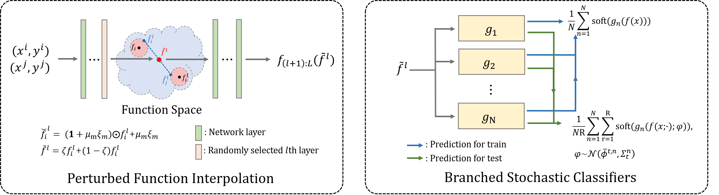
Figure 2: Illustration of Perturbed Function Interpolation (PFI) and Branched Stochastic Classifiers (BSC). PFI randomly perturbs the input, which makes the input loss landscape smooth. For weight perturbation, branched stochastic classifier utilizes weight average along the training trajectory, introduces multiple classifiers, and conduct variational inference during test.

Efficient Optimization for Doubly Perturbed Task-Free Continual Learning

In this section, we propose a novel CL method, called Doubly Perturbed Continual Learning (DPCL), which is inexpensive but very effective to handle the loss (5) with efficient input and weight perturbation schemes. We also design a simple memory management and adaptive learning rate scheme induced by these perturbation schemes.

Perturbed function interpolation

Minimizing the second term in (5) requires gradient for input, which is heavy computation for online learning. From Lim et al. (2022), we design a Perturbed Function Interpolation (PFI), a surrogate of the second term in (5). Let the encoder $f$ consist of $L$-layered networks, denoted by $f=f_{(l+1):L}\circ f_{0:l}$, where $f_{0:l}$ maps an input to the hidden representation at $l$th layer (denoted by $f^{l}$) and $f_{(l+1):L}$ maps $f^{l}$ to the feature space of the encoder $f$. We define the average loss for samples whose label is $y$ as $\bar{\ell}_{y}=\sum_{\tau:y^{\tau}=y}\ell(h(x^{\tau};\theta^{\tau}),y^{\tau})/|\tau:y_{\tau}=y|$. Then, for a randomly selected $l$th layer of $f$, the hidden representation of a sample $(x,y)$ is perturbed by additive and multiplicative noise considering its label as follows:

$$\check{f}^{l}=(\mathbf{1}+\mu_{m}\xi_{m})\odot f^{l}+\mu_{a}\xi_{a},\,\,\xi_{m},\xi_{a}\sim\mathcal{N}(0,I),$$ (6)

where $\mathbf{1}$ denotes the one vector, $\odot$ represents the Hadamard product, $I$ is the identity matrix, $\mu_{m}=\sigma_{m}\tan^{-1}(\bar{\ell}_{y})$, $\mu_{a}=\sigma_{a}\tan^{-1}(\bar{\ell}_{y})$, and $\sigma_{m}$, $\sigma_{a}$ are hyper-parameters. At the iteration where the label $y$ was first encountered, we set $\mu_{m}=\sigma_{m}$ and $\mu_{a}=\sigma_{a}$. Since computing the true $\bar{\ell}_{y}$ is infeasible, we instead update the value by exponential moving average whenever a sample of label $y$ is encountered.

As the main step, the function interpolation can be implemented for the two perturbed feature representations $\check{f}_{i}^{l}$ and $\check{f}_{j}^{l}$ with their labels $y^{i}$ and $y^{j}$, respectively, as follows:

$$(\tilde{f}^{l},\tilde{y})=(\zeta\check{f}_{i}^{l}+(1-\zeta)\check{f}_{j}^{l},\zeta y_{i}+(1-\zeta)y_{j}),$$ (7)

where $\zeta\sim Beta(\alpha,\beta)$, $Beta(\cdot,\cdot)$ is the beta distribution, and $\alpha$ and $\beta$ are hyper-parameters. Finally, the output of the encoder is computed by $f_{(l+1):L}(\tilde{f}^{l})$ and we denote this as $\tilde{f}(\cdot)$. Since the function interpolation requires only element-wise multiplication and addition with samplings from simple distributions, its computational burden is negligible.

Lim et al. (2022) has shown that using perturbation and Mixup in function space can be interpreted as the upper bound of adversarial loss for the input under simplifying assumptions including that the task is binary classification. In this work, we extend it to multi-class classification setup assuming the classifier is linear for each class node and its node is trained in terms of binary classification. Let $\tilde{\mathcal{L}}_{\tau}(\theta)=\ell(g(\tilde{f}(x^{\tau})),y^{\tau})$, the loss computed by the PFI. Suppose that $g$ is a linear classifier for $C$ classes that can be represented as $g=[g_{1},\ldots g_{C}]$ where $g_{c}$ is the sub-classifier connected to the node for the $c$th class, parameterized by $\phi_{c}$.

Proposition 2.

Assume that $\mathcal{L}_{\tau}(\theta)$ is computed by binary classifications for multi-classes. We also suppose $\lVert\nabla_{\theta}h(x^{\tau};\theta)\rVert>0$, $d_{1}\leq\lVert f^{l}_{\tau}\rVert_{2}\leq d_{2}$ for some $0<d_{1}\leq d_{2}$. With more regularity assumptions in Lim et al.(2022),

$$\tilde{\mathcal{L}}_{\tau}(\theta)\geq\max_{\lVert\delta\rVert\leq\epsilon}\ell(h(x^{\tau}+\delta;\theta),y^{\tau})+\mathcal{L}_{\tau}^{\mathrm{reg}}+\epsilon^{2}\psi_{1}(\epsilon),$$ (8)

where $\psi_{1}(\epsilon)\rightarrow 0$ and $\mathcal{L}_{\tau}^{\mathrm{reg}}\rightarrow 0$ as $\epsilon\rightarrow 0$, and $\epsilon$ is assumed to be small and determined by each sample.

In Proposition 2, both $\mathcal{L}_{\tau}^{reg}$ and $\epsilon^{2}\psi_{1}(\epsilon)$ are negligible for small $\epsilon$ and the adversarial loss term becomes dominant in the right side of (8), which validates the use of PFI. See the supplementary materials for the details on Proposition 2.

Methods	CIFAR100 (M=2K)		CIFAR100-SC (M=2K)		ImageNet-100 (M=2K)
	ACC$\uparrow$	FM$\downarrow$	ACC$\uparrow$	FM$\downarrow$	ACC$\uparrow$	FM$\downarrow$
ER  (Rolnick et al. 2019)	36.87$\pm$1.53	44.98$\pm$0.91	40.09$\pm$0.62	30.30$\pm$0.60	22.35$\pm$0.29	51.87$\pm$0.24
EWC++  (Chaudhry et al. 2018a)	36.35$\pm$1.62	44.23$\pm$1.21	39.87$\pm$0.93	29.84$\pm$1.04	22.28$\pm$0.45	51.50$\pm$1.42
DER++ (Buzzega et al. 2020)	39.34$\pm$1.01	40.97$\pm$2.37	41.54$\pm$1.79	29.82$\pm$2.26	25.20$\pm$2.06	52.16$\pm$3.26
BiC (Wu et al. 2019)	36.64$\pm$1.73	44.46$\pm$1.24	38.63$\pm$1.32	29.96$\pm$1.54	22.41$\pm$1.23	50.94$\pm$1.34
MIR (Aljundi et al. 2019a)	35.13$\pm$1.35	45.97$\pm$0.85	37.84$\pm$0.86	31.55$\pm$1.00	22.75$\pm$1.03	52.65$\pm$0.85
CLIB (Koh et al. 2022)	37.48$\pm$1.27	42.66$\pm$0.69	37.27$\pm$1.63	30.04$\pm$1.85	23.85$\pm$1.36	49.96$\pm$1.69
ER-CPR (Cha et al. 2020)	40.98$\pm$0.12	44.47$\pm$0.45	41.93$\pm$0.42	30.67$\pm$0.39	27.08$\pm$3.26	49.93$\pm$1.06
FS-DGPM (Deng et al. 2021)	38.03$\pm$0.58	39.90$\pm$0.39	37.03$\pm$0.57	31.05$\pm$1.63	25.73$\pm$1.68	49.32$\pm$2.03
DRO (Ye and Bors 2022)	39.23$\pm$0.74	41.57$\pm$0.25	39.86$\pm$0.95	27.76$\pm$0.77	27.68$\pm$1.23	39.96$\pm$0.87
ODDL (Wang et al. 2022)	41.49$\pm$1.38	40.01$\pm$0.52	40.82$\pm$1.16	29.06$\pm$1.87	27.54$\pm$0.63	41.23$\pm$1.06
DPCL	45.27$\pm$1.32	37.66$\pm$1.18	45.39$\pm$1.34	26.57$\pm$1.63	30.92$\pm$1.17	37.33$\pm$1.53

Table 1: Results on CIFAR100, CIFAR100-SC, and ImageNet-100. The tasks are distinguished by disjoint sets of classes. For all datasets, we measured averaged accuracy (ACC) and forgetting measure(FM) (%) averaged by 5 different random seeds. Bold and underline indicate the best and the second best performance, respectively.

Branched stochastic classifiers

Minimizing the third term in (5) requires additional gradient steps. We bypass this inspired by ideas from Izmailov et al. (2018),  Maddox et al. (2019), and Wilson and Izmailov (2020), updating multiple models by averaging their weights along training trajectories and performing variational inference by averaging decisions of these models. Cha et al. (2021) confirmed that such stochastic weight averaging effectively flattens the weight loss landscape compared to computing adversarial perturbation directly. In this work, we use this solely for the classifier, termed Branched Stochastic Classifiers (BSC), slightly increasing the parameter count.

Let us first consider a single classifier $g$. Considering the setup of TF-CL, we independently apply the weight perturbation to sub-classifier for each class node in the classifier. Assume that the sub-classifier $\phi_{c}^{t}$ at iteration $t$ follows a multivariate Gaussian distribution with mean $\bar{\phi}_{c}^{t}$ and covariance $\Sigma_{t}^{c}$. With the iteration $T_{c}$ when the model first encounters the class $c$, $\bar{\phi}_{c}^{t}$ and $\Sigma_{t}^{c}$ are updated every $P$ iterations as:

$$\bar{\phi}_{c}^{t}=\frac{k_{c}\bar{\phi}_{c}^{(t-P)}+\phi_{c}^{t}}{k_{c}+1},\Sigma_{t}^{c}=\frac{1}{2}\Sigma_{diag,t}^{c}+\frac{D_{t,c}^{T}D_{t,c}}{2(A-1)},$$ (9)

where $k_{c}=\lfloor{(t-T_{c})/P}\rfloor$ with floor function $\lfloor\cdot\rfloor$, $\Sigma_{diag,t}^{c}=diag(\overline{(\phi_{c}^{t})^{.2}}-(\bar{\phi}_{c}^{t})^{.2})$, $diag(v)$ represents the diagonal matrix with diagonal $v$, and $(\cdot)^{.2}$ is the element-wise square. For (9), $\overline{(\phi_{c}^{t})^{.2}}$ and $D_{t,c}\in\mathbb{R}^{q\times A}$ are updated as:

$$\overline{(\phi_{c}^{t})^{.2}} =\frac{k_{c}\overline{(\phi_{c}^{t-P})^{.2}}+(\phi_{c}^{t})^{.2}}{k_{c}+1},$$

$$D_{t,c} =[D_{t-P,c}[2:A]\,\,(\phi_{c}^{t}-\bar{\phi}_{c}^{t})],$$ (10)

where $D[2:A]\in\mathbb{R}^{q\times(A-1)}$ is the submatrix of $D$ obtained by removing the first column of $D$. For inference, we predict the class probability $p^{t}$ using the variational inference with $\bar{\phi}^{t}=[\bar{\phi}_{1}^{t}\cdots\bar{\phi}_{C}^{t}]$ and $\Sigma_{t}=diag([\Sigma_{t,1}\cdots\Sigma_{t,C}])$ by

$$p^{t}=\frac{1}{R}\sum_{r=1}^{R}\text{soft}(g(f(x;\theta_{e}^{t});\varphi)),\quad\varphi\sim\mathcal{N}(\bar{\phi}^{t},\Sigma_{t}),$$ (11)

where $\text{soft}(\cdot)$ represents the softmax function. Here, we can view the covariance matrix as the low-rank measures on how much each parameter in the classifier deviates by considering each node independently. Note that each of those samplings corresponds to a weight perturbation.

Wilson and Izmailov (2020) verified that both applying deep ensembles and moving average on weights can effectively improve the generalization performance. Since training multiple networks is time-consuming and infeasible in TF-CL setup, we instead introduce multiple linear classifiers $g_{1},\cdots,g_{N}$. By computing the decision $p^{t}_{n}$ for each classifier, the final decision for an input is determined by $\bar{p}^{t}=\frac{1}{N}\Sigma_{n=1}^{N}p^{t}_{n}$. In this case, each network can be viewed as an instance with perturbed weights.

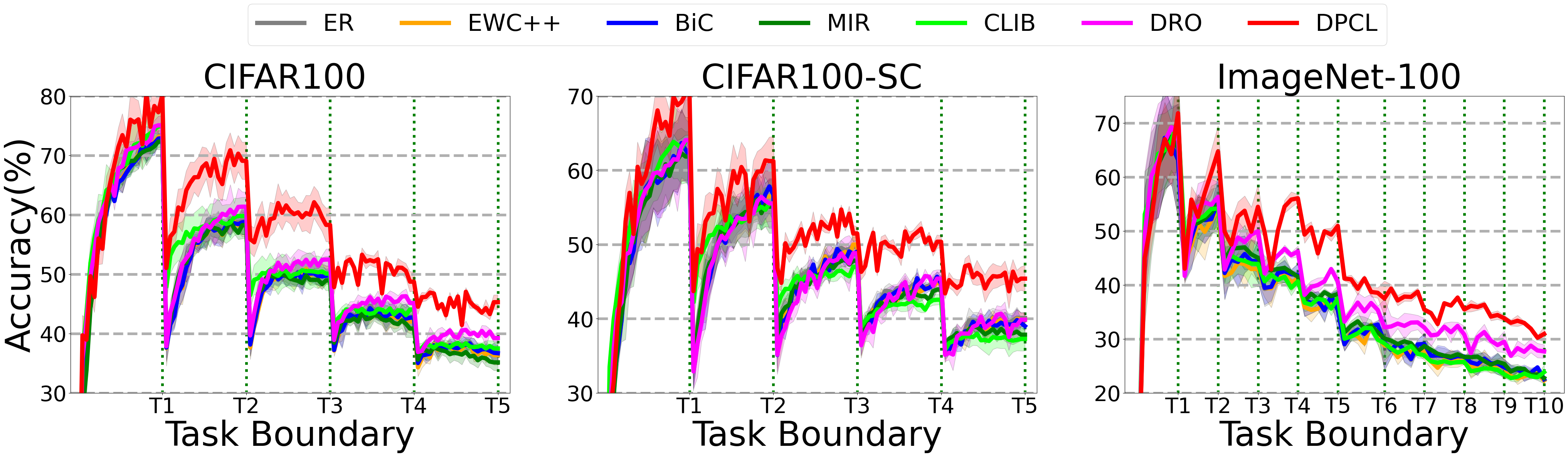
Figure 3: Any-time inference results on CIFAR100, CIFAR100-SC, and ImageNet-100. Each point represents average accuracy over 5 different random seeds and the shaded area represents the standard deviation($\pm$) around the average accuracy.

Perturbation-induced memory management and adaptive learning rate

Several studies have demonstrated that advanced memory management can improve the performance  (Koh et al. 2022; Chrysakis and Moens 2020). Additionally, adjusting learning rate appropriately also enhanced the performance in TF-CL (Koh et al. 2022). To take the same advantages of them, we propose simple yet effective Perturbation-Induced Memory management and Adaptive learning rate (PIMA).

Let $\mathcal{M}_{t}$ be the memory at iteration $t$. For memory management, we basically aim to balance the number of samples for each class in $\mathcal{M}_{t}$ and compute the sample-wise mutual information empirically for a sample $(x,y)$ as

$$\mathbb{I}(x;\phi^{t})=\mathbb{H}(\bar{p}^{t})-\frac{1}{N}\sum_{n=1}^{N}\mathbb{H}(p_{n}^{t}),$$ (12)

where $\mathbb{H}(\cdot)$ is the entropy for a distribution. To manage $\mathcal{M}_{t}$, we introduce a history $H_{t}$ which stores the mutual information for memory samples. Let $H_{t}(x,y)$ be the accumulated mutual information for a memory sample $(x,y)$ at $t$. If $(x,y)$ is selected for training, $H_{t}(x,y)$ is updated by

$$H_{t}(x,y)=(1-\gamma)H_{t-1}(x,y)+\gamma\mathbb{I}(x;\phi^{t}),$$ (13)

where $\gamma\in(0,1)$. Otherwise, $H_{t}(x,y)=H_{t-1}(x,y)$. To update the samples in the memory, we first identify the class $\hat{y}$ that occupies the most in $\mathcal{M}_{t}$. We then compare the values in $\{H_{t}(x,y)|(x,y)\in\mathcal{M}_{t},y=\hat{y}\}$ with $\mathbb{I}(x^{t};\phi^{t})$ for the current stream sample $(x^{t},y^{t})$. If $\mathbb{I}(x^{t};\phi^{t})$ is the smallest, we skip updating the memory. Otherwise, we remove the memory sample of the lowest accumulated mutual information.

We also propose a heuristic but effective adaptive learning rate induced by $H_{t}$. Whenever $\bar{\phi}_{c}^{t}$ is updated, we scale the learning rate $\eta_{t}$ by a factor $\omega>1$ if $\mathbb{E}_{(x,y)\sim\mathcal{M}_{t}}[H_{t}(x,y)]>\mathbb{E}_{(x,y)\sim\mathcal{M}_{t}}[H_{t-1}(x,y)]$ or $\frac{1}{\omega}<1$ otherwise. The algorithm for the memory management and adaptive learning rate are explained in the supplementary materials.

Experiments

Experimental setups

Benchmark datasets. We evaluate our method on three CL benchmark datasets: CIFAR100 (Rebuffi et al. 2017), CIFAR100-SC (Yoon et al. 2019), and ImageNet-100 (Douillard et al. 2020). CIFAR100 and CIFAR100-SC contains 50,000 samples and 10,000 samples for training and test. ImageNet-100 is a subset of ILSVRC2012 with 100 randomly selected classes which consists of about 130K samples for training and 5000 samples for test. For both CIFAR100 and CIFAR100-SC, we split 100 classes into 5 tasks by randomly selecting 20 classes for each task (Rebuffi et al. 2017) and we considered the semantic similarity for CIFAR100-SC (Yoon et al. 2019). For Imagenet-100, we split 100 classes into 10 tasks by randomly selecting 10 classes for each task (Douillard et al. 2020).

Task configurations. We conducted TF-CL experiments on various setups: disjoint, blurry (Bang et al. 2021), and i-blurry (Koh et al. 2022) setups. Disjoint task configuration is the conventional CL setup where any two tasks don’t share common classes to be learned. For more general task configurations, the blurry CL setup involves learning the same classes for all tasks while having different class distributions per task. Meanwhile, in the i-blurry CL setup, each task consists of both shared and disjoint classes, providing more realistic setup than the disjoint and blurry setups.

Baselines. Since most of TF-CL methods are rehearsal-based methods, we compared our DPCL with ER (Rolnick et al. 2019), EWC++ (Chaudhry et al. 2018a), BiC (Wu et al. 2019), DER++ (Buzzega et al. 2020), and MIR (Aljundi et al. 2019a). By EWC++, we combined ER and the regularization approach proposed by Chaudhry et al. (2018a) following the experiments of Koh et al. (2022). We compared DPCL with CLIB (Koh et al. 2022), which was proposed for i-blurry CL setup. We also experimented DRO (Wang et al. 2022), which proposed to perturb the training memory samples via distributionally robust optimization. In our experiments, we evaluate ER-SVGD among the variants of DRO. Lastly, we experimented FS-DGPM (Deng et al. 2021), CPR (Cha et al. 2020) by combining it with ER (ER-CPR), and ODDL (Ye and Bors 2022).

Methods	Blurry (M=2K)		i-Blurry (M=2K)
	ACC$\uparrow$	FM$\downarrow$	ACC$\uparrow$	FM$\downarrow$
ER	24.24$\pm$1.30	20.64$\pm$2.50	39.43$\pm$1.09	15.45$\pm$1.48
EWC++	23.84$\pm$1.57	20.67$\pm$3.34	38.55$\pm$0.79	15.57$\pm$2.36
DER++	24.50$\pm$3.03	17.35$\pm$4.24	44.34$\pm$0.67	13.14$\pm$4.64
BiC	24.96$\pm$1.82	20.12$\pm$3.78	39.57$\pm$0.90	14.23$\pm$2.19
MIR	25.15$\pm$0.08	15.49$\pm$2.07	38.26$\pm$0.63	15.12$\pm$2.69
CLIB	38.13$\pm$0.73	4.69$\pm$0.99	47.04$\pm$0.89	11.69$\pm$2.12
ER-CPR	28.72$\pm$1.67	18.67$\pm$1.23	42.59$\pm$0.66	18.01$\pm$2.68
FS-DGPM	29.72$\pm$0.22	14.51$\pm$2.82	41.99$\pm$0.65	11.81$\pm$0.12
DRO	20.86$\pm$2.45	17.11$\pm$2.47	41.78$\pm$0.42	11.97$\pm$2.79
ODDL	33.35$\pm$1.09	15.12$\pm$1.98	39.71$\pm$1.32	16.12$\pm$1.65
DPCL	47.58$\pm$2.75	11.44$\pm$2.64	50.22$\pm$0.39	11.49$\pm$2.54

Table 2: Results on blurry (Bang et al. 2021) and i-blurry (Koh et al. 2022) setups on CIFAR100. We measured averaged accuracy (ACC) and forgetting measure (FM) (%) averaged by 5 different seeds. Bold and underline indicate the best and the second best performance.

Evaluation metrics. We employ two primary evaluation metrics: averaged accuracy (ACC) and forgetting measure (FM). The averaged accuracy is a commonly used metric in evaluating CL methods (Chaudhry et al. 2018a; Han et al. 2018; Van de Ven and Tolias 2019). Forgetting measure is used to measure how much the average accuracy has dropped from the maximum value for a task  (Yin, Li et al. 2021; Lin et al. 2022). The details for the metric is explained in the supplementary materials.

Implementation details. The overall experiment setting is based on Koh et al. (2022). We used ResNet34 (He et al. 2016) as the base feature encoder for all datasets. We used different batch sizes and update rates for each dataset: CIFAR100 and CIFAR100-SC with a batch size of 16 and 3 updates per sample, ImageNet-100 with a batch size of 64 and 0.25 updates per sample. We used a memory size of 2000 for all datasets. We utilized the Adam optimizer (Kingma and Ba 2015) with an initial learning rate of 0.0003 and applied an exponential learning rate scheduler except CLIB and the optimization configurations reported in the original papers were used for CLIB. We applied AutoAugment (Cubuk et al. 2019) and CutMix (Yun et al. 2019). For DRO, we conducted the CutMix separately for the samples from stream buffer and memory since it conflicts with the perturbation for the memory samples. Since both utilizing CutMix and our PFI is ambiguous, we didn’t apply CutMix for our method. More information for the implementation details can be found in the supplementary materials.

Figure 4: t-SNE on the features at the end of the encoder with CIFAR100. We computed the features and losses for samples in first task after training the last $5$th task. The color represents the loss of a sample (yellow for high loss and purple for low loss). We can see that our DPCL has overall low loss for all regions, especially near the class boundaries.

Methods	One-step (s)	Tr. Time (s)	Model Size	GPU Mem.
ER	0.012	7126	1.00	1.00
EWC++	0.027	16402	2.00	1.23
DER++	0.019	11384	1.00	1.53
BiC	0.015	10643	1.01	1.02
MIR	0.029	18408	1.00	1.96
CLIB	0.061	32519	1.00	4.32
ER-CPR	0.015	8082	1.00	1.00
DRO	0.038	23389	1.00	3.46
ODDL	0.032	22905	2.14	3.31
DPCL	0.017	10925	1.03	1.06

Table 3: Results of runtime/parametric complexity. One-step (s): one-step throughput in second, and Tr. Time (s): total training time in second, Model Size: normalized model size, GPU Mem.: normalized training GPU memory.

Main results

Results on various benchmark datasets We first conducted experiments on CIFAR100, CIFAR100-SC, and ImageNet-100 in a disjoint setup where the classes doesn’t overlap across tasks. As shown in Table  1, DPCL significantly improves the performance on all three datasets. EWC++, BiC, and MIR sometimes enhanced the performance of ER, but the extent of improvement was marginal, as already observed in other studies (Raghavan and Balaprakash 2021; Ye and Bors 2022). Among the baselines, DRO achieved the highest performance on CIFAR100 and ImageNet-100. Interestingly, we observed that for CIFAR100-SC, none of the baselines outperformed ER. CIFAR100-SC is divided into tasks based on their parent classes, and it seems that existing advanced methods have limitations to improve upon ER’s performance for the dataset in the challenging TF-CL scenario. On the other hand, our proposed method significantly outperformed ER for all datasets. Recently, (Koh et al. 2022) argued that inference should be conducted at any-time for TF-CL since the model is agnostic to the task boundaries in practice. They demonstrated that certain methods show significant drop of performance during task learning while they performed well at task boundaries. Based on this observation, we present qualitative results of our method in terms of any-time inference in Fig.  3, where the vertical grids indicate task boundaries. From Fig.  3, our method consistently exhibits the best performance regardless of the iterations during training.

Results on various task configurations. We evaluated our method on various task configurations. For this purpose, we evaluated the performance on CIFAR100 under the blurry  (Bang et al. 2021) and i-blurry setup (Koh et al. 2022). From Table 2, we can observe that ER, EWC, BiC, and MiR show similar performance. CLIB, which is designed for the i-blurry setup, achieved the highest performance among the baselines. In contrast, DRO showed low performance in the blurry setup. On the other hand, our method consistently outperformed the baseline methods by a significant margin in both the blurry and i-blurry setups. Since there exists class imbalance in blurry or i-blurry settings, it empirically shows the robustness of the proposed method to class imbalance.

Runtime/Parametric Complexity Analysis. In Table 3, we evaluated runtime and parametric complexity of the baselines and DPCL. One-step throughput (One-step) and total training time (Training Time) were measured in second for CIFAR100. We also measured model size (Model Size) and training GPU memory (GPU Mem.) on ImageNet-100 after normalizing their values for ER as 1.0. We didn’t consider the memory consumption for replay memory since it is constant for all methods. From Table 3, we can see that our proposed method introduces mild increase on runtime, model size, and training GPU memory compared to other CL methods. Note that DRO, the gradient-based perturbation method, has significantly increased both the training time and memory consumption.

Methods	CIFAR100 (Disjoint)
	ACC$\uparrow$	FM$\downarrow$
DPCL w/o PFI	40.85$\pm$1.68	42.29$\pm$2.32
DPCL w/o BSC	41.75$\pm$1.43	40.56$\pm$1.94
DPCL w/o PIMA	42.94$\pm$1.23	39.79$\pm$2.23
DPCL	45.27$\pm$1.32	37.66$\pm$1.18
BiC	36.64$\pm$1.73	44.46$\pm$1.24
BiC w/ PFI and BSC	43.63$\pm$0.74	38.57$\pm$1.67
CLIB	37.48$\pm$1.27	42.66$\pm$0.69
CLIB w/ PFI and BSC	44.97$\pm$0.97	37.78$\pm$1.24

Table 4: Ablation studies on CIFAR100. PFI and BSC were applied to BiC and CLIB. PIMA was excluded since it conflicts with the baseline methods.

Qualitative Analysis. Fig. 4 shows the t-SNE results for samples within the first task after training the last task under the disjoint setup on CIFAR100. On the t-SNE map, we marked each samples with shade that represents the magnitude of the loss values for the corresponding features. From Fig. 4, we can observe that our method produces much smoother loss landscape for features compared to baselines. It verifies that our method indeed flattens loss landscape in function space. For more experiments for the loss landscape, please refer to the supplementary materials.

Ablation Study. To understand the effect of each component in our DPCL, we conducted an ablation study. We measured the performance of the proposed method by removing each component from DPCL. As shown in Table 4, we observed the obvious performance drop when removing each component, indicating the efficacy of each component of our method. Furthermore, to demonstrate the orthogonality of PFI and BSC to baselines, we applied them to other baselines such as BiC and CLIB. For this, we excluded the previously applied CutMix. Table 4 confirms that the two components of our method can easily be combined with other methods to enhance performance.

Conclusion

In this work, we proposed an optimization framework for Task-Free online CL (TF-CL) and showed that it has an upper-bound which addresses the adversarial input and weight perturbations. Based on the framework, we proposed a method, Doubly Perturbed Continual Learning (DPCL), which employs perturbed interpolation in function space and incorporates branched stochastic classifiers for weight perturbations, with an upper-bound analysis considering adversarial perturbations. By additionally proposing simple memory management scheme and adaptive learning rate induced by the perturbation, we could effectively improve the baseline methods on TF-CL. Experimental results validated the superiority of DPCL over existing methods across various CL benchmarks and setups.

Appendix S1 Doubly Perturbed Task-Free Continual Learning
Supplementary Materials

Algorithms for Doubly Perturbed Continual Learning (DPCL)

In practice, a stream buffer is introduced for TF-CL which can store small number of stream samples. Furthermore, it is conventional to combine the stream buffer with multiple samples from the memory to construct the training batch for rehearsal-based approaches. We summarize the use of Perturbed Function Interpolation with the training batches.

Algorithm 1 Perturbed Function Interpolation with training batches

1:Input training iteration $t$, training batch $B_{t}$, $L$-layered encoder $f$, classifier $g$, mixing parameters $\alpha$ and $\beta$, multiplicative and additive noise factor $\sigma_{m}$ and $\sigma_{a}$, iteration encountered the label $y$ for the first time, $T_{y}$

2:

3:Select a random layer index $l\in\{0,1,\cdots,L\}$

4:$B_{t}^{l}=\{(f_{0:l}(x),y)|(x,y)\in B_{t}\}$

5:$J_{t}=\{i|(f^{l}_{i},y_{i})\in B_{t}^{l}\}$ and $J^{{}^{\prime}}_{t}=\{s_{i}\in J_{t}|i\in J_{t}\}$, where $J^{{}^{\prime}}_{t}$ is the random permutation of $J_{t}$

6:for $(f^{l}_{i},y_{i})\in B_{t}^{l}$ do

7:     if $T_{y_{i}}=t$ then

8:         $\mu_{m}=\sigma_{m}$, $\mu_{a}=\sigma_{a}$

9:     else

10:         $\mu_{m}=\sigma_{m}\text{tan}^{-1}(\ell_{avg}(y_{i}))$, $\mu_{a}=\sigma_{a}\text{tan}^{-1}(\ell_{avg}(y_{i}))$

11:     end if

12:     $B_{t}^{l}\leftarrow B_{t}^{l}\setminus\{(f^{l}_{i},y_{i})\}\cup\{((\mathbf{1}+\mu_{m}\xi_{m})\odot f^{l}_{i}+\mu_{a}\xi_{a},y_{i})\}$, $\xi_{m}\sim\mathcal{N}(0,I)$ and $\xi_{a}\sim\mathcal{N}(0,I)$

13:end for

14:$\tilde{B}_{t}^{l}=\{(\zeta f_{i}^{l}+(1-\zeta)f_{s_{i}}^{l},\zeta y_{i}+(1-\zeta)y_{s_{i}})|(f_{i}^{l},y_{i})\in B_{t}^{l},(f_{s_{i}}^{l},y_{s_{i}})\in B_{t}^{l}\}$, $\zeta\sim Beta(\alpha,\beta)$

15:$F_{t}=\{(f_{(l+1):L}(\tilde{f}),\tilde{y})|(\tilde{f}^{l},\tilde{y})\in\tilde{B}_{t}^{l}\}$

16:Output The network output with PFT, $F_{t}$

We also provide the algorithm for Perturbation-Induced Memory Management and Adaptive Learning Rate in the main paper through Algorithm 2 and Algorithm 3. In similar to Algorithm 1, we consider the stream buffer and training batch based on the memory usage of ER.

Algorithm 2 Perturbation-Induced Memory Management

1:Input training iteration $t$, stream buffer $S_{t}$, memory $\mathcal{M}$, memory budget size $m$, set of training memory samples $M_{t}$, importance history $H_{t}$

2:

3:$\gamma^{\prime}=1-\gamma$

4:for $(x^{i},y^{i})\in M_{t}$ do

5:     $H_{t}(x^{i},y^{i})=\gamma^{\prime}H_{t-1}(x^{i},y^{i})+\gamma\mathbb{I}(x^{i};\phi^{t})$

6:end for

7:for $(x^{\tau},y^{\tau})\in S_{t}$ do

8:     if $|\mathcal{M}|<m$ then

9:         $\mathcal{M}\leftarrow\mathcal{M}\cup\{(x^{t},y^{t})\}$

10:     else

11:         $\bar{y}=\text{arg}\max_{y}|\{(x^{i},y^{i})\in\mathcal{M}|y^{i}=y\}|$

12:         $\mathcal{I}_{y}=\{j|(x^{j},y^{j})\in\mathcal{M},y^{j}=\bar{y}\}$

13:         $\hat{j}=\text{arg}\min_{j\in\mathcal{I}_{y}}H_{t}(x^{j},y^{j})$

14:         if $\mathbb{I}(x^{\tau};\phi^{t})>H_{t}(x^{\hat{j}},y^{\hat{j}})$ then

15:              $\mathcal{M}\leftarrow\mathcal{M}\backslash\{(x^{\hat{j}},y^{\hat{j}})\}\cup\{(x^{\tau},y^{\tau})\}$

16:         end if

17:     end if

18:end for

19:Output $\mathcal{M},H_{t}$

Algorithm 3 Perturbation-Induced Adaptive Learning Rate

1:Input training iteration $t$, memory $\mathcal{M}$, weights of each sub-classifier by moving average $\bar{\phi}_{c}^{t},c\in[1,\cdots,C]$, importance history $H_{t}$, learning rate $\eta_{t}$, multiplicative factor for learning rate schedule $\omega<1$

2:

3:for $c\in[1,\cdots,C]$ do

4:     if $\bar{\phi}_{c}^{t}\neq\bar{\phi}_{c}^{t-1}$ then

5:         if $\mathbb{E}_{\mathcal{M}}[H_{t}]\geq\mathbb{E}_{\mathcal{M}}[H_{t-1}]$ then

6:              $\eta_{t+1}=\omega\eta_{t}$

7:         else

8:              $\eta_{t+1}=\frac{\eta{t}}{\omega}$

9:         end if

10:     end if

11:     End the for loop

12:end for

13:Output $\eta_{t+1}$

Proofs for Propositions

The proposed TF-CL optimization problem in the main paper is

$$\theta^{t}\in\arg\min_{\theta}\,\,\mathcal{L}_{t}(\theta)+\cfrac{\lambda}{t}\textstyle\sum_{\tau=0}^{t-1}(\mathcal{L}_{\tau}(\theta)-\mathcal{L}_{\tau}(\theta^{t-1}))+\rho(\mathcal{L}_{t+1}(\theta^{\prime})-\mathcal{L}_{t+1}(\theta)).$$ (S1)

Let us consider the network $h=g\circ f$ that consists of the encoder $f$ and the classifier $g$, with the parametrization $h(\cdot;\theta)=g(f(\cdot;\theta_{e});\phi)$ where $\theta=[\theta_{e};\phi]$. Suppose that the new parameter $\theta^{\prime}\approx[\theta_{e};\phi^{\prime}]$ has almost no change in the encoder with the future sample $(x^{t+1},y^{t+1})$ while may have substantial change in the classifier. We also define $\eta_{1}^{t}:=\max_{\tau}\lVert x^{t}-x^{\tau}\rVert<\infty,\tau=0,\ldots,t-1,t+1$ and $\eta_{2}^{t}:=\max_{\phi^{\prime}}\lVert\phi^{\prime}-\phi^{t}\rVert$. Then, we have a surrogate of (S1).

Proposition 1.

Assume that $\mathcal{L}_{t}(\theta)$ is Lipschitz continuous for all $t$ and $\phi^{\prime}$ is updated with finite gradient steps from $\phi^{t}$, so that $\phi^{\prime}$ is a bounded random variable and $\eta_{2}^{t}<\infty$ with high probability. Then, the upper-bound for the loss (S1) is

$$\mathcal{L}_{t}(\theta)+\lambda\max_{\lVert\Delta x\rVert\leq\eta_{1}^{t}}\mathcal{L}_{t,\Delta}(\theta)+\rho\max_{\lVert\Delta\phi\rVert\leq\eta_{2}^{t}}\max_{\lVert\Delta x\rVert\leq\eta_{1}^{t}}\mathcal{L}_{t,\Delta}([\theta_{e};\phi^{t}+\Delta\phi]),$$ (S2)

where $\mathcal{L}_{t,\Delta}(\theta)=\ell(h(x^{t}+\Delta x;\theta),y^{t})$.

Proof.

Firstly, an equivalent loss to (S1) is

$$\mathcal{L}_{t}(\theta)+\cfrac{\lambda}{t}\textstyle\sum_{\tau=0}^{t-1}\mathcal{L}_{\tau}(\theta)+\rho(\mathcal{L}_{t+1}(\theta^{\prime})-\mathcal{L}_{t+1}(\theta))=\mathcal{L}_{t}(\theta)+\cfrac{\lambda}{t}\textstyle\sum_{\tau=0}^{t-1}\mathcal{L}_{\tau}(\theta)-\rho\mathcal{L}_{t+1}(\theta)+\rho\mathcal{L}_{t+1}(\theta^{\prime}).$$ (S3)

Then, from the definition of $\eta_{1}^{t}$ and $\mathcal{L}_{\tau}(\theta)\leq\max_{\lVert\Delta x\rVert\leq\eta_{1}^{t}}\mathcal{L}_{t,\Delta}(\theta)$ for all $\tau\in[0,\cdots,t+1]$, we have the bound

$$\cfrac{\lambda}{t}\textstyle\sum_{\tau=0}^{t-1}\mathcal{L}_{\tau}(\theta)-\rho\mathcal{L}_{t+1}(\theta)\leq\lambda\max_{\lVert\Delta x\rVert\leq\eta_{1}^{t}}\mathcal{L}_{t,\Delta}(\theta),$$ (S4)

where $\rho$ is assumed to be positive.

Without loss of generality, we assume that $\theta_{e}$ has no change while $\phi$ may change significantly. Then, we can find the upper-bound for $\rho\mathcal{L}_{t+1}(\theta^{\prime})$ in (S3) as

$$\rho\mathcal{L}_{t+1}(\theta^{\prime})\leq\rho\max_{\lVert\Delta x\rVert\leq\eta_{1}^{t}}\mathcal{L}_{t,\Delta}([\theta_{c};\phi^{\prime}])\leq\rho\max_{\lVert\Delta\phi\rVert\leq\eta_{2}^{t}}\max_{\lVert\Delta x\rVert\leq\eta_{1}^{t}}\mathcal{L}_{t,\Delta}([\theta_{c};\phi+\Delta\phi]).$$ (S5)

From (S3), (S4), and (S5), the upper-bound for the loss function of (S1) is

$$\mathcal{L}_{t}(\theta)+\lambda\max_{\lVert\Delta x\rVert\leq\eta_{1}^{t}}\mathcal{L}_{t,\Delta}(\theta)+\rho\max_{\lVert\Delta\phi\rVert\leq\eta_{2}^{t}}\max_{\lVert\Delta x\rVert\leq\eta_{1}^{t}}\mathcal{L}_{t,\Delta}([\theta_{c};\phi+\Delta\phi]).$$ (S6)

∎

Remark.

Perturbed Feature Interpolation (PFI) is inspired from the Noisy Feature Mixup (NFM)  (Lim et al. 2022). In our approach we inject perturbations on the features proportional to the loss values for each class and then use Mixup (Zhang et al. 2021). On the other hand, NFM applies Mixup first and then perturbations are introduced to the features without considering the class. In other words, for two samples $(x^{i},y^{i})$ and $(x^{j},y^{j})$, the NFM for their features $(f^{l}_{i},y^{i})$ and $(f^{l}_{j},y^{j})$ can be expressed as follows:

$$(\hat{f}^{l},\tilde{y})=((\mathbf{1}+\mu_{m}^{\prime}\xi_{m}^{\prime})\odot\text{Mix}_{\zeta^{\prime}}(f^{l}_{i},f^{l}_{j})+\mu_{a}^{\prime}\xi_{a}^{\prime},\text{Mix}_{\zeta^{\prime}}(y^{i},y^{j}))$$ (S7)

where $\text{Mix}_{\zeta^{\prime}}(a,b)=\zeta^{\prime}a+(1-\zeta^{\prime})b$, $\xi_{m}^{\prime}$ and $\xi_{a}^{\prime}\sim\mathcal{N}(0,I)$, $\zeta^{\prime}\sim Beta(\alpha,\beta)$, and $\mu_{m}^{\prime}$ and $\mu_{a}^{\prime}$ are hyper-parameters for noise scale. Note that we can easily express PFI in the form of NFM by redefining the multiplicative noise scale $\mu_{m}$ and interpolation parameter $\zeta$, which proves that PFI and NFM are indeed equivalent.

From Remark, we can verify that the properties of NFM can be utilized in same way for PFI. One remarkable theorem for NFM can be stated under some regularity conditions for a network (Lim et al. 2022).

Assumption 1.

Assume that the problem is the binary classification with sigmoid activation to compute the probability. Suppose that $\nabla_{f^{l}_{\tau}}h(x^{\tau};\theta)$ and $\nabla_{f^{l}_{\tau}}^{2}h(x^{\tau};\theta)$ exist for all layers, $h(x^{\tau})=\nabla_{f^{l}_{\tau}}h(x^{\tau})^{T}f^{l}_{\tau}$, $\nabla_{f^{l}_{\tau}}h(x^{\tau})=0$ for all $\tau$, and $\mathbb{E}_{\tau}[f^{l}_{\tau}]=0$, $\lVert\nabla_{\theta}h(x^{\tau};\theta)\rVert>0$, $d_{1}\leq\lVert f^{l}_{\tau}\rVert_{2}\leq d_{2}$ for some $0<d_{1}\leq d_{2}$.

Under the Assumption  1,  (Lim et al. 2022) has shown that the loss induced from the NFM is the upper-bound of the loss induced by adversarial perturbation in input space. By utilizing it, we state and prove the following proposition.

Proposition 2.

Suppose that $\mathcal{L}_{\tau}(\theta)=\ell(h(x^{\tau};\theta),y^{\tau})$ is computed by binary classifications for multi-classes and $\tilde{\mathcal{L}}_{\tau}(\theta)$ is the loss computed with PFI. Also, assume that the classifier $g$ is linear for each class and can be represented as $g=[g_{1},\cdots,g_{C}]$ for $C$ classes where $g_{c}$ is the sub-classifier connected to the node for the $c$th class, parameterized by $\phi_{c}$. Then, under the Assumption  1, one can show that

$$\tilde{\mathcal{L}}_{\tau}(\theta)\geq\max_{\lVert\delta\rVert\leq\epsilon}\ell(h(x^{\tau}+\delta;\theta),y^{\tau})+\mathcal{L}_{\tau}^{\mathrm{reg}}+\epsilon^{2}\psi_{1}(\epsilon),$$ (S8)

where $\psi_{1}$ is a function such that $\lim_{\epsilon\rightarrow 0}\psi_{1}(\epsilon)=0$, $\epsilon$ is assumed to be small and determined depending on each sample and perturbations, $\mathcal{L}_{\tau}^{\mathrm{reg}}=\frac{1}{2C}\sum_{c=1}^{C}|S(g_{c}(f(x^{\tau};\theta_{e});\phi_{c}))|(\epsilon^{reg})^{2}$ (detailed form for $\mathcal{L}_{\tau}^{\mathrm{reg}}=\frac{1}{2}|S(h(x^{\tau}))|(\epsilon^{reg})^{2}$ in the main text with the assumption of linear classifier $g$), $S(z)=\frac{e^{z}}{(1+e^{z})^{2}}$, $(\epsilon^{reg})^{2}=\epsilon^{2}\lVert\nabla_{f^{l}}h(x^{\tau};\theta)\rVert_{2}^{2}\psi_{2}(\lambda,\theta,\sigma_{m},\sigma_{a})$, and $\psi_{2}$ is bounded above.

Proof.

Since we consider the binary classification for each class in multi-class classification, we can represent the loss $\mathcal{L}_{\tau}(\theta)$ by the summation of class-wise losses as

$$\mathcal{L}_{\tau}(\theta)=\ell(h(x^{\tau};\theta),y^{\tau})=\frac{1}{C}\sum_{c=1}^{C}\ell(g_{c}(f(x^{\tau};\theta_{e});\phi_{c}),y^{\tau}).$$ (S9)

In a similar way, we can express $\tilde{\mathcal{L}}_{\tau}(\theta)=\frac{1}{C}\sum_{c=1}^{C}\tilde{\mathcal{L}}_{\tau}^{c}(\theta)$ with the class-wise loss $\tilde{\mathcal{L}}_{\tau}^{c}(\theta)$ for perturbed features. From (Lim et al. 2022), we can state an inequality for each class $c$ by

$$\tilde{\mathcal{L}}^{c}_{\tau}(\theta)\geq\max_{\lVert\delta\rVert\leq\epsilon}\ell(g_{c}(f(x^{\tau}+\delta;\theta_{e});\phi_{c}),y^{\tau})+\mathcal{L}_{\tau}^{c,\mathrm{reg}}+\epsilon^{2}\psi_{1}^{c}(\epsilon),$$ (S10)

where $\psi_{1}^{c}$ is a function such that $\lim_{\epsilon\rightarrow 0}\psi_{1}^{c}(\epsilon)=0$, $\epsilon$ is assumed to be small and determined depending on each sample and perturbations, $\mathcal{L}_{\tau}^{c,\mathrm{reg}}=\frac{1}{2}|S(g_{c}(f(x^{\tau};\theta_{e});\phi_{c}))|(\epsilon_{c}^{reg})^{2}$, $S(z)=\frac{e^{z}}{(1+e^{z})^{2}}$, $(\epsilon_{c}^{reg})^{2}=\epsilon^{2}\lVert\nabla_{f^{l}}g_{c}(f(x^{\tau};\theta_{e});\phi_{c})\rVert_{2}^{2}\psi_{2}^{c}(\lambda,\theta,\sigma_{m},\sigma_{a})$, and $\psi_{2}^{c}$ is bounded above. Therefore, we have

$$\tilde{\mathcal{L}}_{\tau}(\theta) \geq\frac{1}{C}\sum_{c=1}^{C}\left(\max_{\lVert\delta\rVert\leq\epsilon}\ell(g_{c}(f(x^{\tau}+\delta;\theta_{e});\phi_{c}),y^{\tau})+\mathcal{L}_{\tau}^{c,\mathrm{reg}}+\epsilon^{2}\psi_{1}^{c}(\epsilon)\right)$$

$$\geq\max_{\lVert\delta\rVert\leq\epsilon}\frac{1}{C}\sum_{c=1}^{C}\ell(g_{c}(f(x^{\tau}+\delta;\theta_{e});\phi_{c}),y^{\tau})+\frac{1}{C}\sum_{c=1}^{C}\mathcal{L}_{\tau}^{c,\mathrm{reg}}+\epsilon^{2}\frac{1}{C}\sum_{c=1}^{C}\psi_{1}^{c}(\epsilon)$$ (S11)

$$\geq\max_{\lVert\delta\rVert\leq\epsilon}\ell(h(x^{\tau}+\delta;\theta),y^{\tau})+\mathcal{L}_{\tau}^{\mathrm{reg}}+\epsilon^{2}\psi_{1}(\epsilon),$$ (S12)

where the second inequality comes from the convexity of $\max$ function and the last inequality is derived by defining $\psi_{2}(\lambda,\theta,\sigma_{m},\sigma_{a})=\min_{c}\psi_{2}^{c}(\lambda,\theta,\sigma_{m},\sigma_{a})$ ∎

Experiment Details

Evaluation metrics. The two primary evaluation metrics in our work is the last average accuracy and forgetting measure. The average accuracy (ACC) can be computed by $A_{t}=\frac{1}{t}\sum_{i=1}^{t}a_{t,i}$ where $a_{t,i}$ is the accuracy for $i$-th task after training $t$-th task. It can measure the overall performance for tasks trained so far, but it is hard to measure the stability and plasticity. By forgetting measure (FM), we measure the drop of the average accuracy from the maximum value for a task  (Yin, Li et al. 2021; Lin et al. 2022). Let $m_{i}^{t}$ be defined as $m_{i}^{t}=|a_{i,i}-a_{t,i}|$. Then, the average forgetting measure $F_{t}$ after training the $t$-th task is defined as $F_{t}=\frac{1}{t-1}\sum_{i=1}^{t-1}m_{i}^{t}$.

The choice of CIFAR100-SC. We chose CIFAR100-SC because it is known to be more challenging than CIFAR100. In CIFAR100-SC, the classes in CIFAR100 are grouped as superclasses to construct tasks. Since the superclasses are semantically different, the domain shift among tasks must be severer than random split of CIFAR100. We included this response in the supplementary material.

Information for baselines. ER (Rolnick et al. 2019) and EWC++ (Chaudhry et al. 2018a) utilize a reservoir sampling for memory management, which involves randomly removing samples from memory to make room for new ones. Additionally, EWC++ incorporates a regularization term in the training loss to penalize the significance of weights, effectively constraining shift of weights. Due to the impracticality of herding selection (Rebuffi et al. 2017) in online CL since it requires access to all task data for computing class mean, we replaced the herding selection in BiC (Wu et al. 2019) with reservoir sampling, following a similar approach described in  (Koh et al. 2022). MIR (Aljundi et al. 2019a) enhances memory utilization by initially selecting a subset of memory that is larger than the size of the training batch. From this subset, samples are chosen based on the expected increase in loss if they were trained with streamed data. This process enables effective model updates. FS-DGPM (Deng et al. 2021) first regulates the flatness of the weight loss landscape of past tasks and dynamically adjusts the gradient subspace for the past tasks to improve the plasticity for new task. CLIB (Koh et al. 2022) is designed to maintain balance of number of samples per class in memory and exclusively utilizes memory for training purposes. A streamed sample can only be trained after it has been stored in memory. ODDL (Ye and Bors 2022) develops a framework that derives generalization bounds based on the discrepancy distance between the visited samples and the entire information accumulated during training. Inspired by this framework, it estimates the discrepancy between samples in the memory and proposes a new sample selection approach based on the discrepancy. DRO (Wang et al. 2022) introduces evolution framework for memory under TF-CL setup by dynamically evolving the memory data distribution that prevents overfitting and handles the high uncertainty in the memory. To achieve this, DRO evolves the memory using Wasserstein gradient flow for the probability measure.

Experiments with Different Number of Splits

Since we fixed the number of splits as 5 and 10 for CIFAR100/CIFAR100-SC and ImageNet100 respectively in the main paper, we experimented with 10/20 splits for CIFAR100/CIFAR100-SC and 5/20 splits for ImageNet100 under the disjoint setup. Table S1 shows that the superiority of the proposed method with different number of splits.

ACC$\uparrow$	CIFAR100		CIFAR100-SC		ImageNet100
Num. Splits	10 Splits	20 Splits	10 Splits	20 Splits	5 Splits	20 Splits
ER  (Rolnick et al. 2019)	34.31$\pm$1.02	31.09$\pm$1.26	36.73$\pm$1.13	34.33$\pm$1.62	28.60$\pm$1.38	20.49$\pm$0.81
DER++ (Buzzega et al. 2020)	34.87$\pm$1.67	33.36$\pm$1.92	36.10$\pm$1.30	35.19$\pm$1.31	29.38$\pm$0.74	18.42$\pm$1.64
CLIB (Koh et al. 2022)	35.88$\pm$1.23	32.27$\pm$1.40	36.62$\pm$0.92	33.82$\pm$1.02	27.65$\pm$0.77	19.51$\pm$0.84
ER-CPR (Cha et al. 2020)	36.31$\pm$0.54	33.79$\pm$0.93	37.82$\pm$0.72	34.01$\pm$2.58	28.86$\pm$0.85	20.70$\pm$1.16
FS-DGPM (Deng et al. 2021)	35.50$\pm$0.72	32.58$\pm$0.82	38.47$\pm$0.84	35.22$\pm$1.07	31.51$\pm$1.29	22.33$\pm$0.73
DRO (Ye and Bors 2022)	37.29$\pm$0.82	35.88$\pm$1.09	38.81$\pm$1.03	36.86$\pm$1.66	32.23$\pm$1.40	24.61$\pm$1.33
ODDL (Wang et al. 2022)	38.23$\pm$1.17	36.27$\pm$1.76	39.12$\pm$1.64	36.39$\pm$1.63	32.44$\pm$1.57	23.71$\pm$0.82
DPCL	40.62$\pm$1.39	38.09$\pm$2.08	41.29$\pm$1.66	38.62$\pm$1.42	33.81$\pm$1.03	26.33$\pm$1.72

Table S1: Accuracies for disjoint setup on CIFAR100, CIFAR100-SC, and ImageNet100 with the various number of splits, averaged by 3 different seeds.

Experiments with Different Blurriness Parameters

With $N_{b}$ and $M_{b}$ being the portion of disjoint classes and the portion of samples of minor classes in a task respectively, we fixed $(N_{b},M_{b})$ as $(0\%,10\%)$ for blurry and $(50\%,10\%)$ for i-blurry setups in Table 2 in the main paper. We explored different values for $M_{b}$ and $N_{b}$ in Table S2 and the proposed method still outperforms the baselines.

ACC$\uparrow$	Blurry		i-Blurry
$(N_{b},M_{b})$	$(0\%,20\%)$	$(0\%,30\%)$	$(25\%,10\%)$	$(75\%,10\%)$
ER	14.28$\pm$1.31	22.83$\pm$1.13	37.96$\pm$1.03	36.93$\pm$0.78
DER++	17.32$\pm$1.04	28.34$\pm$0.84	39.02$\pm$0.98	39.60$\pm$1.01
CLIB	29.02$\pm$0.67	34.87$\pm$0.71	45.23$\pm$1.14	46.02$\pm$0.90
ER-CPR	13.05$\pm$0.89	25.59$\pm$0.87	36.77$\pm$0.82	36.97$\pm$0.73
FS-DGPM	20.43$\pm$0.83	31.81$\pm$1.12	39.92$\pm$0.87	40.45$\pm$0.94
DRO	13.40$\pm$1.72	23.43$\pm$1.94	40.65$\pm$1.16	39.96$\pm$0.89
ODDL	26.04$\pm$1.45	33.28$\pm$1.67	38.65$\pm$0.76	40.13$\pm$0.95
DPCL	35.14$\pm$1.85	43.99$\pm$1.72	47.96$\pm$1.07	47.33$\pm$0.85

Table S2: Accuracies for blurry/i-blurry setups on CIFAR100 with diverse blurriness parameters, averaged by 3 different seeds.

Ablation Studies on Hyper-parameters

The proposed method has some hyper-parameters such as $\alpha$, $\beta$, $\sigma_{a}$, $\sigma_{m}$, and $N$. For all experiments, we fixed $\alpha$$=$$\beta$$=$$1.0$ following Lim et al.(2022) and we have searched for values of $(\sigma_{a},\sigma_{m})$ on CIFAR100 and set $(0.4,0.2)$. Considering trade-off between computation and performance, we set $N=5$. To explore the effect of different values of the hyper-parameters ($\sigma_{a}$, $\sigma_{m}$, $N$), we provide Table S3, which shows that the proposed method is not sensitive to those hyper-parameters.

$\sigma_{a}$	ACC$\uparrow$	$\sigma_{m}$	ACC$\uparrow$	$N$	ACC$\uparrow$
0.1	43.33$\pm$1.28	0.05	44.06$\pm$1.06	1	43.85$\pm$1.90
0.2	44.88$\pm$1.44	0.1	44.73$\pm$1.61	2	44.02$\pm$2.13
0.4	45.27$\pm$1.32	0.2	45.27$\pm$1.32	5	45.27$\pm$1.32
0.8	42.97$\pm$1.98	0.4	44.23$\pm$1.30	10	45.79$\pm$0.51
1.6	41.20$\pm$1.85	0.8	42.39$\pm$1.64	20	46.02$\pm$0.93

Table S3: Accuracies with different values of hyper-parameters for disjoint setup on CIFAR100 averaged by 3 different seeds.

Experiments with ResNet18

Following the setup of Koh et al.(2022), we used ResNet34 for disjoint, blurry, and i-blurry setups in the main paper. Since ResNet18 is also a frequently used architecture, we evaluated our method with ResNet18 on CIFAR100, CIFAR100-SC under disjoint setup and reported the results in Table S4, which shows that the proposed method still outperforms the others.

Methods	CIFAR100		CIFAR100-SC
	ACC$\uparrow$	FM$\downarrow$	ACC$\uparrow$	FM$\downarrow$
ER	35.82$\pm$1.54	43.23$\pm$1.96	37.42$\pm$1.21	32.63$\pm$1.62
DER++	39.01$\pm$1.06	40.12$\pm$2.01	40.99$\pm$0.77	29.18$\pm$1.83
CLIB	36.45$\pm$1.30	39.39$\pm$0.95	38.33$\pm$1.09	29.52$\pm$1.22
ER-CPR	37.09$\pm$1.29	42.03$\pm$2.68	38.12$\pm$1.16	31.55$\pm$1.45
FS-DGPM	37.66$\pm$1.44	39.95$\pm$2.02	38.58$\pm$0.87	30.17$\pm$1.04
DRO	38.97$\pm$0.88	38.12$\pm$1.53	39.00$\pm$1.01	28.29$\pm$1.70
ODDL	40.48$\pm$1.92	38.87$\pm$2.08	41.01$\pm$1.21	28.45$\pm$1.63
DPCL	43.51$\pm$1.71	37.19$\pm$2.74	44.42$\pm$1.41	27.55$\pm$1.92

Table S4: Results with ResNet18 under disjoint setup on CIFAR100 and CIFAR100-SC averaged by 3 different random seeds.

Comparison Experiments of PIMA

Several studies have demonstrated that advanced memory management strategy can improve the performance (Koh et al. 2022; Bang et al. 2021; Chrysakis and Moens 2020). Additionally, adjusting the learning rate appropriately also enhanced the performance in TF-CL (Koh et al. 2022). We proposed PIMA to take the same advantages of them in our proposed doubly perturbed scheme leveraging the network output obtained through PFI and BSC with neglegible computation and memory consumption.

To demonstrate its effectiveness experimentally, we conducted comparison experiments by replacing each element with other baselines. The below Table S5 and Table S6 present the results using other memory management and adaptive learning strategies on disjoint setup for CIFAR100, maintaining the other components of the proposed method, which confirm the efficacy of our PIMA. We added the tables in the supplementary material.

Methods	CLIB	RM	CBRS	Reservoir	DPCL
ACC$\uparrow$	41.13$\pm$0.75	42.24$\pm$0.22	42.24$\pm$0.22	41.75$\pm$0.78	45.27$\pm$1.32
FM$\downarrow$	38.59$\pm$2.08	38.20$\pm$2.43	38.84$\pm$0.75	37.91$\pm$1.55	37.66$\pm$1.18

Table S5: Comparison of memory management schemes on disjoint setup on CIFAR100. We measured averaged accuracy (ACC.) and forgetting measure (FM.) (%) averaged by 5 different seeds.

Methods	CLIB	DPCL
ACC$\uparrow$	43.80$\pm$0.34	45.27$\pm$1.32
FM$\downarrow$	37.39$\pm$0.50	37.66$\pm$1.18

Table S6: Comparison of adaptive learning rate schemes on disjoint setup on CIFAR100. We measured averaged accuracy (ACC.) and forgetting measure (FM.) (%) averaged by 5 different seeds.

Comparison Experiments under the Setup of DRO

In order to demonstrate the effectiveness of our method in different settings, we conducted experiments under the setup of DRO (Wang et al. 2022), especially for comparison with DRO since it is one of the state-of-the-art (SOTA) methods in TF-CL. For this comparison, we conducted the experiments on CIFAR10 and on CIFAR100.

Following of work of Wang et al. (2022), we split CIFAR10 into 5 tasks, set the memory size as 500, and omitted CutMix. For CIFAR100, we split it into 20 tasks and evaluated under various memory sizes (1K, 2K, and 5K) and omitted CutMix. From Table S7, we can see that DPCL consistently outperforms DRO both on CIFAR10 and CIFAR100.

Methods	CIFAR10 (M=500)		CIFAR100 (M=1K)		CIFAR100 (M=2K)		CIFAR100 (M=5K)
	DRO	DPCL	DRO	DPCL	DRO	DPCL	DRO	DPCL
ACC$\uparrow$	50.03$\pm$1.41	55.56$\pm$0.75	18.37$\pm$1.13	24.73$\pm$1.32	27.42$\pm$0.93	27.42$\pm$0.93	24.44$\pm$1.13	29.73$\pm$1.85
FM$\downarrow$	36.22$\pm$2.03	32.93$\pm$1.79	34.32$\pm$1.65	29.29$\pm$1.82	32.42$\pm$2.76	27.55$\pm$1.35	29.31$\pm$2.31	24.08$\pm$1.94

Table S7: Comparison with DRO on disjoint setup on CIFAR10 and CIFAR100 with various memory size. We measured averaged accuracy (ACC.) and forgetting measure (FM.) (%) averaged by 5 different seeds.

Comparison to Architecture-based Methods.

We conducted additional experiments for architecture-based methods on TF-CL, reported in Table S8 and S9. We compared our method with CTN (Pham et al. 2020), evaluated for online CL, and CCLL (Singh et al. 2020), evaluated only for offline CL. To our best knowledge, there’s no architecture-based method for TF-CL, so we conducted them under task-aware setting. The results demonstrate that the proposed method consistently outperforms CTN and CCLL.

Methods	CIFAR100 (M=2K)		CIFAR100-SC (M=2K)		ImageNet-100 (M=2K)
	ACC$\uparrow$	FM$\downarrow$	ACC$\uparrow$	FM$\downarrow$	ACC$\uparrow$	FM$\downarrow$
CTN (Pham et al. 2020)	32.56$\pm$1.76	46.12$\pm$1.93	29.12$\pm$1.56	36.43$\pm$2.62	18.07$\pm$2.08	55.21$\pm$2.82
CCLL (Singh et al. 2020)	29.32$\pm$1.37	47.12$\pm$1.93	27.12$\pm$1.75	37.12$\pm$0.89	17.73$\pm$1.31	54.57$\pm$1.98
DPCL	45.27$\pm$1.32	37.66$\pm$1.18	45.39$\pm$1.34	26.57$\pm$1.63	30.92$\pm$1.17	37.33$\pm$1.53

Table S8: Results of architecture-based methods on CIFAR100, CIFAR100-SC, and ImageNet-100 on disjoint setup. For all datasets, we measured averaged accuracy (ACC) and forgetting measure(FM) (%) averaged by 5 different random seeds.

Methods	Blurry (M=2K)		i-Blurry (M=2K)
	ACC$\uparrow$	FM$\downarrow$	ACC$\uparrow$	FM$\downarrow$
CTN	26.72$\pm$0.67	21.51$\pm$2.13	33.75$\pm$1.78	23.65$\pm$2.31
CCLL	25.12$\pm$2.07	22.34$\pm$1.64	28.18$\pm$1.03	26.19$\pm$1.35
DPCL	47.58$\pm$2.75	11.44$\pm$2.64	50.22$\pm$0.39	11.49$\pm$2.54

Table S9: Results of architecture-based methods on blurry (Bang et al. 2021) and i-blurry (Koh et al. 2022) setups on CIFAR100. We measured averaged accuracy (ACC.) and forgetting measure(FM.) (%) averaged by 5 different seeds.

Analysis on Weight Loss Landscape for Classifier

From experiments in main paper, we analyzed the loss landscape on the function space of the first task data after training the fifth task. Through t-SNE visualization, we observed that our DPCL has relatively smaller loss values for the samples compared to the baselines, particularly showing a clear gap at class boundaries where the loss values are usually large. This indicates that our approach makes the function space smoother. To observe the sharpness of the classifier’s weight loss landscape, we perturbed the weights of the trained classifier and examined how the loss values changed. In order to exclude the network’s scaling invariance, we normalized the randomly sampled direction $\mathbf{d}$ from a Gaussian distribution using $\mathbf{d}\leftarrow\frac{\mathbf{d}}{\lVert\mathbf{d}\rVert_{F}}\lVert\phi\rVert_{F}$ (Deng et al. 2021). The experiments were performed by averaging results over 5 random seeds.

Figure S1 shows the loss landscapes after training the first, third, and fifth tasks on the first task data. Our DPCL exhibits the flattest loss landscape in all cases. Additionally, in Figure S1 (b) and (c), our DPCL consistently achieves the lowest loss across all regions. Note that among the baselines, ER exhibits the flattest loss landscape. This suggests that the existing methods are not necessarily related to flattening the classifier’s weight loss landscape and can even deteriorate it. While DRO (Wang et al. 2022) made the function space smoother in the experiments in the main paper by perturbing the input space, it does not exhibit favorable characteristics for the classifier’s weight loss landscape.

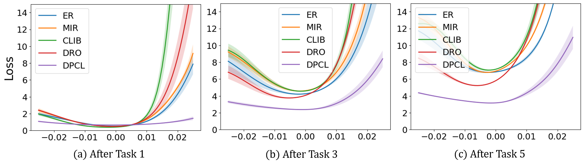
Figure S1: Weight loss landscape for data from first task after training for (a) first, (b) third, and (c) fifth task on CIFAR100 dataset. We randomly selected the direction for perturbation and averaged results from 5 random seeds. We can see that our DPCL has the flattest weight loss landscape for all cases and the lowest loss values at the origin.

References

- Ahn et al. (2021) Ahn, H.; Kwak, J.; Lim, S.; Bang, H.; Kim, H.; and Moon, T. 2021. Ss-il: Separated softmax for incremental learning. ICCV, 844–853.
- Aljundi et al. (2019a) Aljundi, R.; Caccia, L.; Belilovsky, E.; Caccia, M.; Lin, M.; Charlin, L.; and Tuytelaars, T. 2019a. Online Continual Learning with Maximally Interfered Retrieval. NeurIPS, 11849–11860.
- Aljundi, Kelchtermans, and Tuytelaars (2019) Aljundi, R.; Kelchtermans, K.; and Tuytelaars, T. 2019. Task-free continual learning. CVPR, 11254–11263.
- Aljundi et al. (2019) Aljundi, R.; Lin, M.; Goujaud, B.; and Bengio, Y. 2019. Gradient based sample selection for online continual learning. NeurIPS.
- Bang et al. (2021) Bang, J.; Kim, H.; Yoo, Y.; Ha, J.-W.; and Choi, J. 2021. Rainbow memory: Continual learning with a memory of diverse samples. CVPR, 8218–8227.
- Buzzega et al. (2020) Buzzega, P.; Boschini, M.; Porrello, A.; Abati, D.; and Calderara, S. 2020. Dark experience for general continual learning: a strong, simple baseline. NeurIPS, 33: 15920–15930.
- Carpenter and Grossberg (1987) Carpenter, G. A.; and Grossberg, S. 1987. ART 2: Self-organization of stable category recognition codes for analog input patterns. Applied optics, 26(23): 4919–4930.
- Cha et al. (2021) Cha, J.; Chun, S.; Lee, K.; Cho, H.-C.; Park, S.; Lee, Y.; and Park, S. 2021. Swad: Domain generalization by seeking flat minima. NeurIPS, 22405–22418.
- Cha et al. (2020) Cha, S.; Hsu, H.; Hwang, T.; Calmon, F.; and Moon, T. 2020. CPR: Classifier-Projection Regularization for Continual Learning. ICLR.
- Chaudhry et al. (2018a) Chaudhry, A.; Dokania, P. K.; Ajanthan, T.; and Torr, P. H. 2018a. Riemannian walk for incremental learning: Understanding forgetting and intransigence. ECCV, 532–547.
- Chaudhry et al. (2021) Chaudhry, A.; Gordo, A.; Dokania, P.; Torr, P.; and Lopez-Paz, D. 2021. Using hindsight to anchor past knowledge in continual learning. AAAI, 35: 6993–7001.
- Chaudhry et al. (2018b) Chaudhry, A.; Ranzato, M.; Rohrbach, M.; and Elhoseiny, M. 2018b. Efficient Lifelong Learning with A-GEM. ICLR.
- Chrysakis and Moens (2020) Chrysakis, A.; and Moens, M.-F. 2020. Online continual learning from imbalanced data. ICML, 1952–1961.
- Cubuk et al. (2019) Cubuk, E. D.; Zoph, B.; Mane, D.; Vasudevan, V.; and Le, Q. V. 2019. Autoaugment: Learning augmentation strategies from data. CVPR, 113–123.
- Deng et al. (2021) Deng, D.; Chen, G.; Hao, J.; Wang, Q.; and Heng, P.-A. 2021. Flattening sharpness for dynamic gradient projection memory benefits continual learning. NeurIPS, 34: 18710–18721.
- Douillard et al. (2020) Douillard, A.; Cord, M.; Ollion, C.; Robert, T.; and Valle, E. 2020. Podnet: Pooled outputs distillation for small-tasks incremental learning. ECCV, 86–102.
- Foret et al. (2020) Foret, P.; Kleiner, A.; Mobahi, H.; and Neyshabur, B. 2020. Sharpness-aware Minimization for Efficiently Improving Generalization. ICLR.
- Han et al. (2018) Han, B.; Yao, Q.; Yu, X.; Niu, G.; Xu, M.; Hu, W.; Tsang, I.; and Sugiyama, M. 2018. Co-teaching: Robust training of deep neural networks with extremely noisy labels. NeurIPS, 31.
- He et al. (2016) He, K.; Zhang, X.; Ren, S.; and Sun, J. 2016. Deep residual learning for image recognition. CVPR, 770–778.
- He et al. (2020) He, X.; Sygnowski, J.; Galashov, A.; Rusu, A. A.; Teh, Y. W.; and Pascanu, R. 2020. Task Agnostic Continual Learning via Meta Learning. 4th Lifelong Machine Learning Workshop at ICML.
- Hung et al. (2019) Hung, C.-Y.; Tu, C.-H.; Wu, C.-E.; Chen, C.-H.; Chan, Y.-M.; and Chen, C.-S. 2019. Compacting, picking and growing for unforgetting continual learning. NeurIPS, 32.
- Izmailov et al. (2018) Izmailov, P.; Wilson, A.; Podoprikhin, D.; Vetrov, D.; and Garipov, T. 2018. Averaging weights leads to wider optima and better generalization. UAI, 876–885.
- Jin et al. (2021) Jin, X.; Sadhu, A.; Du, J.; and Ren, X. 2021. Gradient-based editing of memory examples for online task-free continual learning. NeurIPS, 34: 29193–29205.
- Jung et al. (2023) Jung, D.; Lee, D.; Hong, S.; Jang, H.; Bae, H.; and Yoon, S. 2023. New Insights for the Stability-Plasticity Dilemma in Online Continual Learning. ICLR.
- Jung et al. (2020) Jung, S.; Ahn, H.; Cha, S.; and Moon, T. 2020. Continual learning with node-importance based adaptive group sparse regularization. NeurIPS, 3647–3658.
- Keskar et al. (2017) Keskar, N. S.; Mudigere, D.; Nocedal, J.; Smelyanskiy, M.; and Tang, P. T. P. 2017. On Large-Batch Training for Deep Learning: Generalization Gap and Sharp Minima. ICLR.
- Kingma and Ba (2015) Kingma, D. P.; and Ba, J. 2015. Adam: A Method for Stochastic Optimization. ICLR.
- Kirkpatrick et al. (2017) Kirkpatrick, J.; Pascanu, R.; Rabinowitz, N.; Veness, J.; Desjardins, G.; Rusu, A. A.; Milan, K.; Quan, J.; Ramalho, T.; Grabska-Barwinska, A.; et al. 2017. Overcoming catastrophic forgetting in neural networks. PNAS, 114(13): 3521–3526.
- Koh et al. (2022) Koh, H.; Kim, D.; Ha, J.-W.; and Choi, J. 2022. Online Continual Learning on Class Incremental Blurry Task Configuration with Anytime Inference. ICLR.
- Lim et al. (2022) Lim, S. H.; Erichson, N. B.; Utrera, F.; Xu, W.; and Mahoney, M. W. 2022. Noisy Feature Mixup. ICLR.
- Lin et al. (2022) Lin, S.; Yang, L.; Fan, D.; and Zhang, J. 2022. Beyond not-forgetting: Continual learning with backward knowledge transfer. NeurIPS, 35: 16165–16177.
- Lopez-Paz and Ranzato (2017) Lopez-Paz, D.; and Ranzato, M. 2017. Gradient episodic memory for continual learning. NeurIPS, 30.
- Lyu, Huang, and Liang (2015) Lyu, C.; Huang, K.; and Liang, H.-N. 2015. A unified gradient regularization family for adversarial examples. ICDM, 301–309.
- Maddox et al. (2019) Maddox, W. J.; Izmailov, P.; Garipov, T.; Vetrov, D. P.; and Wilson, A. G. 2019. A simple baseline for bayesian uncertainty in deep learning. NeurIPS, 32.
- Madry et al. (2017) Madry, A.; Makelov, A.; Schmidt, L.; Tsipras, D.; and Vladu, A. 2017. Towards deep learning models resistant to adversarial attacks. arXiv:1706.06083.
- Mallya, Davis, and Lazebnik (2018) Mallya, A.; Davis, D.; and Lazebnik, S. 2018. Piggyback: Adapting a single network to multiple tasks by learning to mask weights. ECCV, 67–82.
- Mallya and Lazebnik (2018) Mallya, A.; and Lazebnik, S. 2018. Packnet: Adding multiple tasks to a single network by iterative pruning. CVPR, 7765–7773.
- McCloskey and Cohen (1989) McCloskey, M.; and Cohen, N. J. 1989. Catastrophic interference in connectionist networks: The sequential learning problem. Psychology of learning and motivation, 24: 109–165.
- Mermillod, Bugaiska, and Bonin (2013) Mermillod, M.; Bugaiska, A.; and Bonin, P. 2013. The stability-plasticity dilemma: investigating the continuum from catastrophic forgetting to age-limited learning effects. Frontiers in psychology, 4: 504.
- Moosavi-Dezfooli et al. (2019) Moosavi-Dezfooli, S.-M.; Fawzi, A.; Uesato, J.; and Frossard, P. 2019. Robustness via curvature regularization, and vice versa. CVPR, 9078–9086.
- Neyshabur et al. (2017) Neyshabur, B.; Bhojanapalli, S.; McAllester, D.; and Srebro, N. 2017. Exploring generalization in deep learning. NeurIPS, 30.
- Pham et al. (2020) Pham, Q.; Liu, C.; Sahoo, D.; and Steven, H. 2020. Contextual transformation networks for online continual learning. ICLR.
- Pourcel, Vu, and French (2022) Pourcel, J.; Vu, N.-S.; and French, R. M. 2022. Online Task-free Continual Learning with Dynamic Sparse Distributed Memory. ECCV, 739–756.
- Qin et al. (2019) Qin, C.; Martens, J.; Gowal, S.; Krishnan, D.; Dvijotham, K.; Fawzi, A.; De, S.; Stanforth, R.; and Kohli, P. 2019. Adversarial robustness through local linearization. NeurIPS, 32.
- Raghavan and Balaprakash (2021) Raghavan, K.; and Balaprakash, P. 2021. Formalizing the generalization-forgetting trade-off in continual learning. NeurIPS, 34: 17284–17297.
- Rebuffi et al. (2017) Rebuffi, S.-A.; Kolesnikov, A.; Sperl, G.; and Lampert, C. H. 2017. icarl: Incremental classifier and representation learning. CVPR, 2001–2010.
- Rolnick et al. (2019) Rolnick, D.; Ahuja, A.; Schwarz, J.; Lillicrap, T.; and Wayne, G. 2019. Experience replay for continual learning. NeurIPS, 32.
- Ross and Doshi-Velez (2018) Ross, A.; and Doshi-Velez, F. 2018. Improving the adversarial robustness and interpretability of deep neural networks by regularizing their input gradients. AAAI, 32.
- Serra et al. (2018) Serra, J.; Suris, D.; Miron, M.; and Karatzoglou, A. 2018. Overcoming catastrophic forgetting with hard attention to the task. ICLR, 4548–4557.
- Shin et al. (2017) Shin, H.; Lee, J. K.; Kim, J.; and Kim, J. 2017. Continual learning with deep generative replay. NeurIPS, 30.
- Shmelkov, Schmid, and Alahari (2017) Shmelkov, K.; Schmid, C.; and Alahari, K. 2017. Incremental learning of object detectors without catastrophic forgetting. ICCV, 3400–3409.
- Singh et al. (2020) Singh, P.; Verma, V. K.; Mazumder, P.; Carin, L.; and Rai, P. 2020. Calibrating cnns for lifelong learning. Advances in Neural Information Processing Systems, 33: 15579–15590.
- Van de Ven and Tolias (2019) Van de Ven, G. M.; and Tolias, A. S. 2019. Three scenarios for continual learning. arXiv preprint arXiv:1904.07734.
- Wang et al. (2021) Wang, L.; Zhang, M.; Jia, Z.; Li, Q.; Bao, C.; Ma, K.; Zhu, J.; and Zhong, Y. 2021. Afec: Active forgetting of negative transfer in continual learning. NeurIPS, 22379–22391.
- Wang et al. (2022) Wang, Z.; Shen, L.; Fang, L.; Suo, Q.; Duan, T.; and Gao, M. 2022. Improving task-free continual learning by distributionally robust memory evolution. ICML, 22985–22998.