Spin wave confinement in hybrid superconductor-ferrimagnet nanostructure

Abstract

Eddy currents in a superconductor shield the magnetic field in its interior and are responsible for the formation of a magnetic stray field outside of the superconducting structure. The stray field can be controlled by the external magnetic field and affect the magnetization dynamics in the magnetic system placed in its range. In the case of a hybrid system consisting of a superconducting strip placed over a magnetic layer, we predict theoretically the confinement of spin waves in the well of the static stray field. The number of bound states and their frequencies can be controlled by an external magnetic field. We have presented the results of semi-analytical calculations complemented by numerical modeling.

I Introduction

The states of superconductivity and ferromagnetism are very rarely observed in a single material. Their intrinsic co-existence (i.e. in one uniform phase, for the same electrons) was found for triplet pairing in a proximity to a magnetic quantum critical point (e.g. for ${\rm UGe_{2}}$) [1, 2]. The other possibility, known for long time and more conventional [3, 4], is the coexistence of two phases where large and localized moments of 4f electrons (Er, Gd) provide long-range strong ferromagnetism whereas 3d conduction electrons are responsible for superconductivity.

The hybrid systems [5, 6, 7, 8], where superconductor and ferromagnet are part of the same structure and interact with each other, usually offer much more flexibility both in design and implementation of new features. The superconductor/ferromagnet hybrids can be divided into two categories – where both subsystems are in direct contact [9] or separated by non-magnetic non-conducting material. In the latter case, the coupling at a distance results from the fact that both the eddy currents in the superconductor and the magnetic moments in the ferromagnet generate a magnetic field. The coupling provided by the magnetic field can be controlled by the external magnetic field as well as be tailored by the geometry, since both the distribution of the eddy currents and the magnetization configuration depend on these factors.

In electromagnetically-coupled hybrids, the ferromagnet can modify the properties of the superconductor, e.g. the magnetic screening can increase the value of critical current density in the superconductor [10], or presence of the stray field produced by ferromagnetic nanoelements can affect the nucleation of vortices [11] or pin and guide the vortices in the superconductor [12]. Similarly, the presence of the superconductor can have influence on the ferromagnet, e.g. by controlling the magnetization dynamics [13]. In this research field, we can find the reports about induction of magnonic crystals and nonreciprocal spin wave (SW) transmission in uniform magnetic layer due to the screening of dynamic demagnetizing field by a superconductor [14], enhancement of nonlinear SW dynamics [15], Bragg scattering of SWs on the field produced by Abrikosov vortex lattice [16, 17], or SW generation by moving vortices [18, 19, 20]. Undoubtedly, superconductor/ferromagnet hybrids offer many possibilities for controlling the dynamics of SWs. One of the topics not fully explored is the problem of localization of SWs in these systems.

In this study, we conduct a theoretical and numerical investigation of the SW confinement induced in a uniform ferrimagnetic (FM) layer by the stray field of a superconducting (SC) strip. We demonstrate that by adjusting the applied field, we can impact on the depth of the stray field well and thereby control the number and frequencies of the confined SW modes.

II Model

The considered hybrid system consists of gallium-doped yttrium iron garnet (Ga:YIG) FM thin film and Nb SC strip in the Meissner state, electrically isolated from each other by thin non-magnetic spacer (see Fig. 1). According to the Meissner effect, a SC strip expels a magnetic field from its volume by means of eddy currents. These currents create a non-uniform distribution of the magnetic field throughout the entire space, including the FM film. Such geometry enables the investigation of the coupling between FM and SC subsystems as purely classical, where the stray magnetic field from the eddy currents in SC strip impacts the magnetization in FM layer.

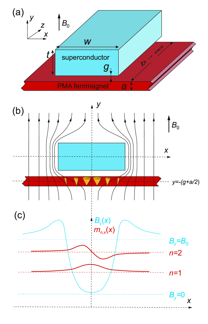
Figure 1: (a) A thin FM film ($a=20$ nm) is exposed to the stray field of a rectangular SC strip ($w=400$ nm, $t=100$ nm). The ferrimagnet (Ga:YIG) and the superconductor (Nb) are separated by a small gap ($g=10$ nm). The magnetic film has low $M_{\rm s}$ and exhibits PMA, so it is magnetized out of plane in the absence of the external magnetic field. The sketches (b,c) illustrate the mechanism of SW localization. (b) The static internal magnetic field is lowered in the region of the ferrimagnet underneath the SC strip. This leads to the confinement of SW modes (c), which are quantized in the quasi-parabolic well of the internal field.

The system is placed in an external magnetic field perpendicular to the FM layer. In Ga:YIG, the shape anisotropy is overcome by the perpendicular magnetic anisotropy (PMA), leading to the magnetization being directed out of plane even in the absence of external magnetic field. Operating with the relatively small external field, we can sustain the Meissner state in confined geometry of the strip, and observe the impact of the stray field of SC strip on the magnetization dynamics in FM layer. Then, the stray field of SC strip is tuned by the external field and induces the well of static effective field of controllable depth in the FM layer. The well can confine the SWs of the frequencies lower than the ferromagnetic resonance (FMR) frequency of FM layer in the absence of SC strip.

A uniformly-magnetized infinite FM layer does not produce outside any static stray field – only the internal demagnetizing field ($-M_{\rm s}\hat{\mathbf{y}}$) is present. However, the stray field of SC strip induces a weak magnetization texture in FM layer, close to SC strip edges. It can produce a static stray field, although it is small and can be neglected – see Section S1 in Supplemental Material. The dynamic stray field coming from the SW modes in FM layer can be also considered as negligible. For FM layer magnetized in the out-of-plane direction, the dynamic components of magnetization are tangential to the surfaces and do not produce any surface magnetic charges. On the other hand, the dynamic stray field can be generated by the volume magnetic charges but it requires a strong non-uniformity of the SW profile, which is observed for the higher SW modes (not investigated here). Therefore, we assume that eddy currents are unaffected by SWs and remain constant. To sum up, both static and dynamic stray fields induced in FM layer are negligible for the SC strip. Therefore, there is no need to solve self-consistent problem for our system and take into account the mutual interaction between the FM layer and the SC strip.

Taking these assumptions into account, our studies were carried out in two stages. We first calculated the static stray field generated by the SC strip. It was determined from the distribution of SC currents, which was found by a semi-analytical solution of the London equations. The static field generated by SC strip was then included as a correction to the effective field to Landau-Lifshitz (LL) equation. The LL equation was solved both semi-analytically and numerically and was used to find the confined SW modes.

II.1 The static magnetic field produced by superconducting strip

The London equation has been solved analytically for a number of geometries, such as a film [21], a cylindrical wire [22] and an infinitely-thin cylindrical dot [23]. However, the analytical solution of the London equation presents difficulties, even for such a simple structure as a strip, due to the impossibility of variable separation. We have therefore used the semi-analytical method developed by Brandt [24, 25]. For the SC strip in an external field applied along the $y$-direction $\mathbf{B}_{0}=B_{0}\hat{\mathbf{y}}$, the Meissner effect induces a current of density $\mathbf{J}=J(x,y)\hat{\mathbf{z}}$ flowing along the $z$-axis and generating a stray field $\mathbf{B}_{\rm sc}(x,y)$, which lacks $z$-component – see Fig. 1(b). According to the Ampere law, we can relate the current density to the total field $\mathbf{B}$ and vector potential $\mathbf{A}$:

$$\mu_{0}\mathbf{J}=\nabla\times\mathbf{B}=\nabla\times\nabla\times\mathbf{A}=-\Delta\mathbf{A},$$ (1)

where we used the Coulomb gauge ($\nabla\cdot\mathbf{A}=0$), and the symbol $\mu_{0}$ denotes the permeability of vacuum. Eq. (1) can be interpreted as two-dimensional Poisson equation for vector potential $\mathbf{A}=A(x,y)\hat{\mathbf{z}}$ with a current $\mathbf{J}=J(x,y)\hat{\mathbf{z}}$ being a source:

$$\Delta A(x,y)=-\mu_{0}J(x,y),$$ (2)

where $\Delta$ is a two-dimensional Laplacian. Let’s decompose the vector potential $\mathbf{A}=(xB_{0}+A_{\rm sc}(x,y))\hat{\mathbf{z}}$ into the contribution related to uniform external field: $\mu_{0}xH_{0}$ and the field produced by SC: $A_{\rm sc}(x,y)$ and then relate the latter inside SC to a current $J(x,y)$ by London equation with Coulomb gauge:

$$A_{\rm sc}(x,y)=-\mu_{0}\lambda^{2}J(x,y),$$ (3)

where $\lambda$ is London penetration depth. Then, using Eq. (3), we can write Eq. (2) in the following integral form:

$$\lambda^{2}J(x,y)\!=\!\!\!\iint_{S}dx^{\prime}dy^{\prime}Q(x,y,x^{\prime},y^{\prime})J(x^{\prime},y^{\prime})+\!xH_{0},$$ (4)

where $S$ is the cross-section of the SC strip in $xy$-plane and the function $Q=\tfrac{1}{2\pi}\ln(\sqrt{(x-x^{\prime})^{2}+(y-y^{\prime})^{2}})$ is the integral kernel for two-dimensional Laplace operator.

Equation (4) can be integrated numerically by sampling the function $J(x,y)$ on a square grid of equidistant points $(x_{i},y_{j})$: $x_{i}=((i-\tfrac{1}{2})/N_{x}-\tfrac{1}{2})w$, $y_{j}=((j-\tfrac{1}{2})/N_{y}-\tfrac{1}{2})t$, where $w$ and $t$ are the strip width and thickness respectively (see Fig. 1) and $N_{x}$ and $N_{y}$ are number of points in $x$- and $y$-direction, where $N_{x}/w\approx N_{y}/t$ and $i=1,\ldots,N_{x}$, $j=1,\ldots,N_{y}$. By marking the points $\mathbf{r}_{l}=(x_{i},y_{j})$ with an index $l=1,\ldots,N\!=\!N_{x}N_{y}$, the function $J(x,y)$ becomes a vector $J_{l}$ with $N$ components, and the integral kernel is transformed into the $N\times N$ matrix $Q_{l,l^{\prime}}$. Note that $Q_{l,l^{\prime}}$ diverges for $l=l^{\prime}$, which should be avoided. Eq. (4) for the density current distribution $J(x,y)$ can then be rewritten in a matrix form:

$$\lambda^{2}J_{l}=\sum_{l^{\prime}}\tilde{Q}_{l,l^{\prime}}J_{l^{\prime}}+\frac{1}{\mu_{0}}x_{l^{\prime}}B_{0},$$ (5)

where $\tilde{Q}_{l,l^{\prime}}=Q_{l,l^{\prime}}\frac{w}{N_{x}}\frac{t}{N_{y}}$. The solution of Eq. (5) for $J_{l}$ can be found when we invert the matrix $P_{l,l^{\prime}}=\lambda^{2}\delta_{l,l^{\prime}}-\tilde{Q}_{l,l^{\prime}}$:

$$J_{l}=\frac{1}{\mu_{0}}B_{0}\sum_{l^{\prime}}(P^{-1})_{l,l^{\prime}}x_{l^{\prime}}.$$ (6)

Finally, the distribution of the field $B_{\rm sc}$ produced by eddy currents can be determined using the Biot-Savart law:

$$\begin{split}B_{{\rm sc},x}(x,y)=\frac{\mu_{0}}{2\pi}\iint_{S}dx^{\prime}dy^{\prime}\frac{J(x^{\prime},y^{\prime})(y^{\prime}-y)}{(x^{\prime}-x)^{2}+(y^{\prime}-y)^{2}},\\ B_{{\rm sc},y}(x,y)=-\frac{\mu_{0}}{2\pi}\iint_{S}dx^{\prime}dy^{\prime}\frac{J(x^{\prime},y^{\prime})(x^{\prime}-x)}{(x^{\prime}-x)^{2}+(y^{\prime}-y)^{2}},\end{split}$$ (7)

where the integrals in Eq. (7) can be calculated numerically by sampling the current density $J$ on the cross-section $S$ of SC strip.

II.2 The spin-wave modes confined in the well of magnetic field induced by superconducting strip

After calculating the stray field generated by the SC strip, the next step is to investigate the SW localization in the FM layer placed under the strip. Two assumptions were made in our theoretical model: (i) our calculations have shown that the magnetic field generated by the SC strip does not vary significantly across the thin FM layer, so we assume that the SC field does not depend on the $y$-coordinate and is equal to the value at the film center; (ii) we have neglected the tangential component of the SC field and, consequently, the deviation of the magnetization from the film normal, so we have included only the normal component of the SC field, which is responsible for the formation of the well for localized SW modes, and thus considered the uniform magnetization directed perpendicular to the film plane.

The magnetization dynamics in continuous medium is described semi-classically by the LL equation:

$$\frac{\partial\mathbf{M}(\mathbf{r},t)}{\partial t}=-|\gamma|\mu_{0}\mathbf{M}(\mathbf{r},t)\times\mathbf{H}_{\rm eff}(\mathbf{r},t),$$ (8)

where $\gamma$ is gyromagnetic ratio and $\mathbf{H}_{\rm eff}$ is effective magnetic field, calculated from the free energy density $F$ [26]:

$$\begin{split}F=-(\mathbf{B}_{0}+\mathbf{B}_{\rm sc})\cdot\mathbf{M}+\frac{A_{\rm ex}}{M_{\rm s}^{2}}(\nabla\mathbf{M})^{2}\\ -\frac{1}{2}\mu_{0}\mathbf{H}_{\rm d}\cdot\mathbf{M}-\frac{K_{\rm u}}{M_{\rm s}^{2}}(\mathbf{M}\cdot\hat{\mathbf{n}})^{2}\end{split}$$ (9)

with respect to magnetization: $\mathbf{H}_{\rm eff}=-\frac{1}{\mu_{0}}\frac{\delta F}{\delta\mathbf{M}}$. Also, in Eq. (8), we neglected the damping. The material parameters in Eq. (9): $M_{\rm s}$, $A_{\rm ex}$, $K_{\rm u}$ denote the saturation magnetization, exchange stiffness constant and uniaxial anisotropy, respectively. In our case, the magnetocrystalline anisotropy is easy-axis anisotropy ($K_{\rm u}>0$), oriented in the out-of-plane direction ($\hat{\mathbf{n}}=\hat{\mathbf{y}}$) which overcome the shape anisotropy ($K_{\rm u}>\mu_{0}M^{2}_{\rm s}/2$). The demagnetizing field is non-local (which means that $\mathbf{H}_{\rm d}(\mathbf{r},t)$ at specific point $\mathbf{r}$ depends on the magnetization distribution in the whole magnetic body). We use the linear approximation, where the magnetization precesses harmonically around the equilibrium position $\mathbf{M}_{0}(\mathbf{r})=M_{\rm s}\hat{\mathbf{y}}$ with the amplitude $\mathbf{m}(\mathbf{r})=m_{x}\hat{\mathbf{x}}+m_{z}\hat{\mathbf{z}}$ much smaller than the static magnetization component ($|\mathbf{m}(\mathbf{r})|\ll M_{\rm s}$), giving the total magnetization vector $\mathbf{M}(\mathbf{r},t)\approx\mathbf{M}_{0}(\mathbf{r})+\mathbf{m}(\mathbf{r})e^{i\omega t}$. Then, we can decompose the demagnetizing field to static and dynamic component $\mathbf{H}_{\rm d}(\mathbf{r},t)\approx-M_{\rm s}\hat{\mathbf{y}}+\mathbf{h}_{\rm d}(\mathbf{r})e^{i\omega t}$, where the dynamic component $\mathbf{h}_{\rm d}=h_{\mathrm{d},x}\hat{\mathbf{x}}+h_{\mathrm{d},z}\hat{\mathbf{z}}$ can be written in a general form:

$$\mathbf{h}_{\rm d}(\mathbf{r})=-\nabla\int_{V}dv^{\prime}\mathbf{m}(\mathbf{r}^{\prime})\cdot\nabla^{\prime}\frac{1}{4\pi|\mathbf{r}-\mathbf{r}^{\prime}|}.$$ (10)

The LL equation (8) can be then written in the linearized form:

$$\begin{split}\;\;i\omega\;m_{x}(x)=&|\gamma|\left[\left(B_{0}-\mu_{0}M_{\rm s}+\frac{2K_{u}}{M_{\rm s}}+B_{{\rm sc},y}(x)\right)m_{z}(x)\right.\\ &-\left.\frac{2A_{\rm ex}}{M_{\rm s}}\frac{d^{2}}{dx^{2}}m_{z}(x)-\mu_{0}M_{\rm s}h_{{\rm d},z}(x)\right],\\ -i\omega\;m_{z}(x)=&|\gamma|\left[\left(B_{0}-\mu_{0}M_{\rm s}+\frac{2K_{u}}{M_{\rm s}}+B_{{\rm sc},y}(x)\right)m_{x}(x)\right.\\ &-\left.\frac{2A_{\rm ex}}{M_{\rm s}}\frac{d^{2}}{dx^{2}}m_{x}(x)-\mu_{0}M_{\rm s}h_{{\rm d},x}(x)\right],\end{split}$$ (11)

where we used the assumption that inside the thin FM layer both magnetization and field are constant in an out-of-plane direction, i.e. do not depend on $y$-coordinate, and the tangential component of the stray field of SC can be neglected: $B_{{\rm sc},x}\approx~{}0$.

In most cases, it is impossible to obtain a rigorous analytical solution of LL equation for the SWs in nanostructures. Usually the eigenfunctions of the exchange field operator, which, however, are not eigenfunctions of the operator for demagnetizing field, are used as trial functions in Ritz method. Such an approach, when applied to planar nanoelements with relatively uniform magnetization distribution, allows to obtain the solutions which are close to the exact ones [27, 28, 29, 30]. In these systems, the demagnetizing field is almost constant in the whole volume (due to the small magnetic volume charges), except the vicinity of the edges (where surface magnetic charges play role). However, such an approach does not work in a case of nanoelements with strongly inhomogeneous demagnetizing or external fields. In such cases, it is necessary to consider trial solutions being the eigenfunctions of the operator, which is a sum of the exchange operator and the operators which express the impact of demagnetizing effects or external fields. For instance, the SW localization in tangentially-magnetized thin layer induced by the dipolar stray field of magnetic sphere was considered in [31]. In this system, the static stray field of the sphere, perceptible by the SW in FM layer, was approximated by parabolic functions. In the framework of this approximation, the linearized LL equation was reduced to the system of coupled Schrödinger-like equations for quantum harmonic oscillator with dynamic demagnetizing field of FM layer considered as a perturbation [31, 32, 33]. Therefore, the eigenfunctions in the form of Hermite polynomials could be chosen as trial solutions for SW modes.

Considering the assumptions made at the beginning of Sec. II, we can use the approach proposed in Ref. [31] for investigating SC-FM hybrid system. The linearized LL equation can be then written in a compact form:

$$\begin{split}\;\;i\omega\;m_{x}(x)&=|\gamma|\big{(}\Xi(x)m_{z}(x)-\mu_{0}M_{\rm s}h_{{\rm d},z}(x)\big{)},\\ -i\omega\;m_{z}(x)&=|\gamma|\big{(}\Xi(x)m_{x}(x)-\mu_{0}M_{\rm s}h_{{\rm d},x}(x)\big{)}.\end{split}$$ (12)

The operator $\Xi(x)=-\tfrac{2A_{\rm ex}}{M_{\rm s}}\tfrac{d^{2}}{dx^{2}}+B_{y}(x)$ describes the impact of dynamic exchange field and total static field:

$$B_{y}(x)=\!B_{0}-\mu_{0}M_{\rm s}+\frac{2K_{\rm u}}{M_{\rm s}}+\underbrace{B_{0}(\beta_{0}+\beta_{2}x^{2}+O(x^{2}))}_{B_{{\rm sc},y}(x)},$$ (13)

on magnetization dynamics. It is worth noting that, according to Eqs. (6) and (7), the stray field $B_{{\rm sc},y}(x)$ is linearly scaled by external field $B_{0}$.

By introducing the circular polarization for dynamic component of magnetization: $m=m_{z}+im_{x}$ and neglecting the dynamic demagnetizing field $\mathbf{h}_{\rm d}$, we can transform the set of equations (12) into the form equivalent to the stationary Schrödinger equation:

$$\Xi(x)\,m_{n}(x)=\frac{1}{|\gamma|}\omega_{0,n}m_{n}(x).$$ (14)

Equation (14) can be solved analytically after neglecting higher-order terms in the expansion in Eq. (13). The problem is then reduced to the magnonic counterpart of quantum harmonic oscillator with equidistant eigenfrequencies $\omega_{0,n}$ and corresponding eigenfunctions $m_{n}(x)$ expressed by Hermite polynomials $H_{n}(\xi)~{}=~{}(-1)^{n}\exp(\xi^{2})\tfrac{d^{n}}{d\xi^{n}}\exp(-\xi^{2})$:

$$m_{n}(\xi=Kx)=CM_{\rm s}\underbrace{\frac{1}{\sqrt{2^{n}n!\sqrt{\pi}}}\exp(-\xi^{2})H_{n}(\xi)}_{\psi_{n}(\xi)}$$ (15)

for every $n^{\rm th}$ SW mode. The scaling factor $K=\sqrt[4]{B_{0}\,\beta_{2}\,\tfrac{M_{\rm s}}{2A_{\rm ex}}}$ expresses the interplay between the strength of exchange interaction and the curvature (strength) of the well of SC stray field, in which the SW modes are confined. The real function $\psi_{n}(\xi)$ is normalized: $\int_{-\infty}^{\infty}\psi_{n}(\xi)=1$ and dimensionless constant $C$ expresses the complex SW amplitude.

The approximation $B_{{\rm sc},y}(x)\approx B_{0}(\beta_{0}+\beta_{2}x^{2})$ is not valid for wide SC strips: $w\gg\lambda$ (where the well $B_{{\rm sc},y}(x)$ becomes relatively flat at the bottom) and narrow strips: $w<\lambda$ or small $B_{0}$ (where the well is shallow and distortion of its parabolic shape, related to the presence of the barriers on its sides, affects the mode of the lowest frequency). Therefore, we solve Eq. (14) numerically for the stray field $B_{{\rm sc},y}$ in a full form given by Eq. (7) – this task is relatively simple and does not demand extensive computations. The obtained frequencies $\tilde{\omega}_{0,n}\neq{\omega}_{0,n}$ of bound SW modes were calculated for realistic (i.e. non-parabolic) stray field of SC strip but with dynamic dipolar interaction neglected. However, we used the approximated (by Hermite polynomials) profiles of the eigenmodes from Eq. (15) to include the role of dynamic dipolar interactions.

The next step in our computational procedure is to include the impact of the dynamic demagnetizing field $\mathbf{h}_{\rm d}$ and correct the frequencies of individual modes $\tilde{\omega}_{0,n}$ calculated in the absence of $\mathbf{h}_{\rm d}$. We are going to limit our calculations to so-called diagonal approximation [33], which was satisfactory for many similar cases [32, 31], where the difference between successive frequencies $\tilde{\omega}_{0,n}$ is large with respect to frequency shift due to dynamic dipolar interaction. This approximation neglects also the inter-mode dipolar coupling. According to Eq. (10), the dynamic demagnetizing field produced by a single mode can be written in a form:

$$h_{{\rm d},p,n}(x)=-\int_{V}dv^{\prime}\sum_{q}m_{q,n}(x^{\prime})\frac{d^{2}}{dpdq^{\prime}}\frac{1}{4\pi|\mathbf{r}-\mathbf{r}^{\prime}|},$$ (16)

were the indices $p$ and $q$ run over the coordinates $x$ and $z$, and derivative $\frac{d}{dq^{\prime}}$ means $\frac{d}{dx^{\prime}}$ (or $\frac{d}{dz^{\prime}}$) for $q=x$ (or $q=z$). The symbol $m_{q,n}(x)$ denotes the components of dynamic magnetization for $n^{\rm th}$ mode.

The spectrum of eigenmodes, which includes the correction resulting from the presence of dynamic dipolar interaction, has the following form (see Appendix A for derivation):

$$\omega_{n}\!=\!\sqrt{\big{(}\tilde{\omega}_{0,n}\!-\!|\gamma|\mu_{0}M_{\rm s}\langle\tilde{h}_{{\rm d},x}\rangle_{n}\big{)}\big{(}\tilde{\omega}_{0,n}\!-\!|\gamma|\mu_{0}M_{\rm s}\langle\tilde{h}_{{\rm d},z}\rangle_{n}\big{)}},$$ (17)

where $\langle\tilde{h}_{{\rm d},p}\rangle_{n}$ are averaged and normalized (dimensionless) components of $\mathbf{h}_{\rm d}$. The averaged field $\langle\tilde{h}_{{\rm d},z}\rangle_{n}$ is equal to zero in considered system, whereas $\langle\tilde{h}_{{\rm d},x}\rangle_{n}$ can be expressed by the compact formula (see Ref. [31] and Appendix B):

$$\langle\tilde{h}_{{\rm d},x}\rangle_{n}\!\approx-\frac{1}{K}\int_{-\infty}^{\infty}\!dk_{x}\left(1\!-\!\frac{1-e^{-k_{x}a}}{k_{x}a}\right)\tilde{\psi}_{n}\left(\frac{k_{x}}{K}\right),$$ (18)

where $\tilde{\psi}_{n}(\mathcal{K})=\tfrac{1}{\sqrt{2\pi}}\int_{-\infty}^{\infty}e^{-i\mathcal{K}\xi}\psi_{n}(\xi)d\xi$ is the Fourier transform of $\psi(\xi)$. The one-dimensional integral in Eq. (18) is relatively simple to compute in comparison with the calculations of $\langle\tilde{h}_{{\rm d},u}\rangle_{n}$ directly from Eq. (16). It is worth noting that we approximate $m_{p,n}(x)$ by taking $m_{p,n}(x)\approx C_{p}M_{\rm s}\psi_{n}(Kx)$ where $\psi_{n}(Kx)$ are eigenfunctions of $\Xi(x)$. The amplitudes $C_{p}$ are canceled during the normalization – see Appendix B.

Micromagnetic simulations

To perform micromagnetic simulations we used the open-source environment Mumax3 [34] that solves LL equation using finite-difference method in the time domain. We discretized the system with a regular mesh with unit cell $2\times 20\times 20$ nm³ (along the $x$, $y$, and $z$-axis respectively). The system was placed in an inhomogeneous external magnetic field $\mathbf{B}_{0}+\mathbf{B}_{\rm sc}(\mathbf{r})$ that includes the full contribution of the stray field of SC strip. The field profile was imported from an external file containing the results of semi-analytic calculations of $\mathbf{B}_{\rm sc}(\mathbf{r})$. We applied the periodic boundary conditions along the $z$-axis (1024 repetitions) to simulate an infinitely-long strip. We increased the damping constant close to the edges of the domain perpendicular to $x$-axis from $\alpha_{\mathrm{edge}}=0$ to $0.5$ in order to eliminate the reflections along $x$-axis edges. The SWs in the system were numerically excited by a rectangular model-antenna of width $12$ nm, placed in the center of the film. The antenna generated a local dynamic magnetic field described with the function $H_{\mathrm{ant}}(t)=H_{0}\mathrm{sinc}(2\mathrm{\pi}f_{\mathrm{cut}}(t-t_{0}))\hat{x}$, where $\mu_{0}H_{0}=0.024B_{0}$, $f_{\mathrm{cut}}$ is a cutoff frequency that varies in the simulations depending on the depth of the well of stray field $\Delta B_{{\rm sc},y}$ – see Fig. 2(a). In each case of different $\Delta B_{{\rm sc},y}$, the simulation was run for the timespan $1000/f_{\mathrm{cut}}$. The results of simulations were saved continuously as the snapshots of magnetic configuration with time sampling $t_{\mathrm{sample}}=0.5/(1.5f_{\mathrm{cut}})$. In the postprocessing, all saved magnetic configurations were used to calculate the spectra by employing the Fourier transform. The visualizations of particular modes in the system were done by calculating the inverse Fourier transform of frequencies corresponding to the modes.

The micromagnetic simulations were also used to calculate the stray field produced by magnetization texture in FM layer resulting from the action of a stray field from SC strip – see Section S1 in Supplemental Material.

Finite-element method

Numerical simulations were performed in COMSOL Multiphysics using finite-element method in order to calculate the stray field coming from the SC strip subjected to the external magnetic field. To be consistent with the semi-analytical calculations, we used London equation

$$\Delta A=\frac{1}{\lambda^{2}}A$$ (19)

inside the SC material and Ampere law

$$\Delta A=0$$ (20)

outside of the SC material, both modified to the form for magnetic vector potential $A$. We investigated the system in two-dimensional model in $xy$-plane. In this case, the Coulomb gauge $\nabla\cdot\mathbf{A}=0$ and the condition on the SC boundary $\mathbf{A}\cdot\hat{n}=0$ are automatically fulfilled. External magnetic field $B_{0}$ was applied as a boundary condition $-\partial_{x}A=B_{0}$ far away from the SC material. Here, the SC strip was placed in the center of 100 $\mu$m square-shaped cell, on which boundary this condition is applied.

We have checked the validity of London model for considered SC structure by finite-element method calculation of the stray field based on Ginzburg-Landau model – see Section S2 in Supplemental Material.

III Results

We considered SC strip of the thickness $t=100$ nm and width $w=400$ (or $800$ nm, for comparison). The strip was made of Nb for which we assumed the London penetration depth $\lambda=50$ nm [35]. The SC strip was placed over the FM layer of thickness $a=20$ nm and separated from its top surface by the non-magnetic and non-conducting spacer of thickness $g=10$ nm – see Fig. 1. The FM layer, made of Ga:YIG, was characterized by the following values of material parameters: saturation magnetization $M_{\rm s}=16$ kA/m, exchange stiffness $A_{\mathrm{ex}}=1.37$ pJ/m and gyromagnetic ratio $\gamma=179$ GHz/T. The Ga:YIG layer can have a strong PMA [36]. We assumed the realistic value of the uniaxial anisotropy $K_{\mathrm{u}}=756$ J/$\mathrm{m}^{3}$, which ensures the out-of-plane orientation of magnetization even in the absence of external magnetic field. For micromagnetic simulations, we included the magnetization damping constant for Ga:YIG $\alpha=0.001$. For semi-analytical calculations the damping was neglected.

III.1 Stray field of superconducting strip

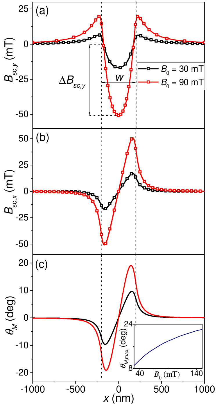
Figure 2: The profiles of the magnetic field components (a) $B_{{\rm sc},y}$ and (b) $B_{{\rm sc},x}$ produced by SC strip, calculated using Eq. (7) (solid lines) and using numerical simulations (square dots). (c) The deflection $\theta_{M}$ of the magnetization from the direction of external field $\mathbf{B}_{0}=B_{0}\hat{\mathbf{y}}$. The inset plot shows the evolution of the maximum angle deviation with the external magnetic field value. All profiles (a,b,c) are plotted along the line $y=0$, passing through the center of the strip: $(x,y)=(0,0)$. Dashed vertical lines mark the edges of SC strip. Black and red lines correspond to the external field $B_{0}$ equal to 30 mT and 90 mT, respectively. Please note that to calculate the total magnetic field, we have to add $\mathbf{B}_{0}$ and $\mathbf{B}_{{\rm sc}}$.

Figure 2(a,b) presents the profiles of the $y$-component (Fig. 2(a)) and $x$-component (Fig. 2(b)) of the stray field $\mathbf{B}_{\rm sc}$ produced by SC strip of the width $w=400$ nm for two selected values of out-of-plane applied field: $B_{0}=30$ mT (black lines) and $90$ mT (red lines). The profiles are the $x$-coordinate dependencies calculated for fixed $y=y_{0}=-(t/2+g+a/2)=-70$ nm, i.e. in the middle of the FM film. The dependencies $B_{{\rm sc},y}(x)$, $B_{{\rm sc},x}(x)$ are consistent with the expected onion-like shape of the field around SC strip (see Fig. 1(b)). The well of $B_{{\rm sc},y}(x)$ is a signature of the screening of external field $\mathbf{B}_{0}=B_{0}\hat{\mathbf{y}}$ by the cost of the increase of the field close to the edges of the strip (vertical dashed lines in Fig. 2). On the other hand, the in-plane component of the stray field $B_{{\rm sc},x}$ reflects the deflection of the magnetic field lines by-passing the SC strip. This effect is the strongest in the proximity of the strip edges. The stray field was calculated semi-analytically using Eq. (7) – (red and black lines in Fig. 2(a,b)), and obtained results were successfully cross-checked using finite-element method calculations – (red and black square dots in Fig. 2(a,b)). Eq. (7) and the plots in Figs. 2(a,b) show that the stray field is linearly scalable with the external field $B_{0}$. While we increase $B_{0}$ from 30 mT to 90 mT, the magnitude of the profiles $B_{{\rm sc},y}(x)$, $B_{{\rm sc},x}(x)$ are increasing exactly three times – see Eqs. (6) and (7).

In the absence of the SC strip, the static magnetization is oriented out of plane due to the PMA in Ga:YIG layer but the in-plane component $B_{{\rm sc},x}$ tilts magnetization from the layer’s normal – see Fig.2(c). Surprisingly, the angle between the magnetization and the applied field’s direction increases with the increase of the magnitude of applied field. However, it is understandable if we keep in mind that the in-plane component of the stray field, which is responsible for the magnetization tilting, increases with the applied field: $B_{{\rm sc},x}\propto B_{0}$ – see Fig. 2(b). The angle, at which magnetization is deflected from out-of-plane direction $\theta_{M}(x)$ (Fig.2(c)), can be calculated by finding minimum of the free energy density (9) for successive positions $x$. Our calculations have shown that the inhomogeneous exchange interaction caused by non-collinear magnetization texture does not significantly influence the value of the magnetization deviation angle. Therefore, to estimate angle $\theta_{M}$, we considered the free magnetic energy density of the film in an external magnetic field applied at an angle $\theta_{B}$ neglecting exchange interaction:

$$\begin{split}F(\theta)=&-BM_{s}\cos(\theta-\theta_{B})\\ &+\tfrac{1}{2}\mu_{0}M_{\rm s}\cos^{2}(\theta)-K_{\rm u}\cos^{2}(\theta)\end{split}$$ (21)

where the angle $\theta$ is trial orientation of the magnetization for which we look for a minimum of $F(\theta)$ at every position $x$ independently. The angle $\theta=\theta_{M}$ corresponding to the minimum: $F_{\rm min}=F(\theta_{M})$ determines the equilibrium orientation of the magnetization. The first term in Eq. (21) corresponds to the Zeeman interaction with total magnetic field, the second one describes the demagnetizing energy (shape anisotropy), and the third one corresponds to the energy related to the out-of-plane uniaxial anisotropy. It is worth noting that both the magnitude $B(x)=|\mathbf{B}_{0}+\mathbf{B}_{\rm sc}(x)|$ and the angle $\theta_{B}(x)={\rm arctan}[B_{{\rm sc},x}(x)/(B_{0}+B_{{\rm sc},y}(x))]$ of total static magnetic field are position-dependent.

The minimization of Eq. (21) results in an equation for the local magnetization angle $\theta_{M}(x)$ as a function of the $x$-coordinate. For relatively small values of the angles $\theta-\theta_{B}$ and $\theta$, the trigonometric functions in Eq. (21) can be expanded in Taylor series which results in the polynomial equation for $\theta_{M}$:

$$\begin{split}\frac{1}{\mu_{0}}B\left[(\theta_{M}-\theta_{B})-\frac{1}{6}(\theta_{M}-\theta_{B})^{3}\right]\\ +\left(\frac{2K_{u}}{M_{s}}-M_{s}\right)\left[\theta_{M}-\frac{2}{3}\theta^{3}\right]=0,\end{split}$$ (22)

which is relatively easy to solve. For larger values of the applied field $B_{0}$ and related deflection angles, the equilibrium orientation $\theta_{M}(x)$ must be found numerically. The inset plot in Fig. 2(c) shows evolution of the maximum angle deviation $\theta_{M,\rm{max}}$ with the value of applied magnetic field $B_{0}$.

It should be noted that the formation of non-collinear magnetization texture allows the SW excitation by an alternating magnetic field applied along the external static field $\mathbf{B}_{0}$. In this case, the SW modes will only be excited in the regions below the edges of the SC strips, where the static magnetization is tilted.

Two-dimensional maps of the stray field $\mathbf{B}_{{\rm sc}}$ are shown in Section S2 in Supplemental Material, comparing maps calculated from the London model to those obtained through the solution of Ginzburg-Landau equations. Our results show that for the assumed value of $\lambda$ = 50 nm, we are able to keep the Meissner state for the field $B_{0}=30$ mT, and moreover, the results of the London model are almost the same as the results for the Ginzburg-Landau model.

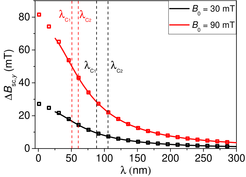
Figure 3: The depth of the well of SC field $\Delta B_{{\rm sc},y}$ (see Fig. 2(a)) as a function of London penetration depth $\lambda$ calculated using Eq. (7) (solid lines) and numerical simulations (square dots). The black and red lines correspond to two different values of the external field $B_{0}=30$ mT and 90 mT, respectively. Dashed vertical lines show critical values of $\lambda$ for Meissner ($\lambda_{C1}$) and mixed ($\lambda_{C2}$) states for $B_{0}=30$ mT and 90 mT in the Ginzburg-Landau model assuming $\kappa=1$.

London penetration depth $\lambda$ is a crucial parameter, which determines efficiency of the magnetic field screening by SC material. To understand how $\lambda$ influences on the condition for the SW localization, we have calculated the depth of the well $B_{{\rm sc},y}(x)$ (see Fig. 2(a)) as a function of $\lambda$ for the width of SC strip $w=400$ nm and two selected values of the external field $B_{0}=30$ mT (black lines and squares) and 90 mT (red line and squares) – see Fig. 3. Semi-analytical calculations performed with the help of Eq. (7) (solid lines) are in perfect agreement with results of numerical simulations (square dots) for $\lambda>20$ nm, while for smaller value of $\lambda$ semi-analytical computations faces difficulties since they require the bulk cell size to be much smaller than $\lambda$, what demands a significant increase of the number of cells and time-consuming computations. The dependencies $\Delta B_{{\rm sc},y}(\lambda)$ were presented in Fig. 3. It is evident that the decrease of $\Delta B_{{\rm sc},y}$ with increasing $\lambda$ is a manifestation of the gradual disappearance of SC properties, which is revealed as a weakening stray field that allows the external field to penetrate deeper into the SC strip. However, this picture becomes more complicated when we consider the more general theory of superconductivity described by Ginzburg-Landau model which allows the phase transitions to mixed and normal phase at the critical fields $B_{C1}$ and $B_{C2}$, respectively, for type-II superconductors like Nd. Taking into account the critical fields dependencies on material parameters: penetration depth $\lambda$ and correlation length $\xi$, we should look for the critical values of material parameters for which the Meissner state or superconductivity at all is destroyed. To estimate critical values of $\lambda$, we have used the formulas for critical fields of a bulk SC: $B_{C2}=\Phi_{0}/(2\pi\xi)$ and $B_{C1}=B_{C2}\kappa/\sqrt{2}$ (where $\Phi_{0}$ is magnetic flux quantum) and we set $\kappa=\xi/\lambda=1$ (which is in the range of experimental values for Nb $0.85<\kappa<1.3$ [37]). For $B_{0}=30$ mT, $\lambda_{C1}=88$ nm and $\lambda_{C2}=105$ nm (black dashed lines in Fig. 3). It guarantees the Meissner state and justify the usage London’s theory, which were confirmed by numerical calculations according to the Ginzburg-Landau theory (see Section S2 in Supplemental Material). For $B_{0}=90$ mT, $\lambda_{C1}=51$ nm and $\lambda_{C2}=90$ nm (red dashed lines in Fig. 3). Taking into account that these values are approximate, there is no guarantee that obtained results for $B_{0}=90$ mT can be observed experimentally.

In general, the London penetration depth is not only material-specific but depends also on the sample shape and dimensions. It was shown in Ref. 35 that a decrease of the sample size leads to an increase of $\lambda$. In our theoretical calculations we took $\lambda=50$ nm, which is not far from the experimental value [35].

III.2 The spin-wave modes confined in the well of magnetic field induced by superconducting strip

Figure 4 presents the SW profiles of the modes localized in the well of effective field produced by the SC strip, for the external fields: $B_{0}=10$ mT (Fig. 4(c)), 30 mT (Fig. 4(a,d)) and 90 mT (Fig. 4(b,e)). The profiles were computed numerically with the help of Mumax3 software (light red solid lines) and calculated using the semi-analytical model (red dashes lines). The blue lines show FMR frequency of homogeneous film at certain $B_{0}$ fields in the absence of the SC strip. Left and right columns in Fig. 4 correspond to the width of SC strip $w=400$ nm (Fig. 4(a,b)) and 800 nm (Fig. 4(c,d,e)), respectively. For larger value of external field $B_{0}$, the well $B_{{\rm sc},y}(x)$ is deeper (see Fig. 2(a)) and can accommodate more SW modes. However, there is an upper limit for $B_{0}$ caused by phase transition at $B_{C1}$. Our model, based on London’s theory, does not include the existence of mixed state, which can appear in the considered range of external field $B_{0}$. The presence of vortices will modify the stray field produced by the SC strip which will be important in the experimental implementation of investigated system. However, the ultimate limit is given by the second critical field[38]. On the other hand, the field $B_{0}=10$ mT is too small for the strip of width $400$ nm to create a well which is deep enough to confine SW modes. For the external fields $B_{0}=30$ mT (Fig. 4(a)) or $90$ mT (Fig. 4(b)) the well is sufficiently deep to bond one or two SW modes (solid and dashed lines) of the frequencies lower than FMR frequency of homogeneous film (horizontal blue line). Another strategy for SW binding is to widen the SC strip and thus widen the related well of the stray field.

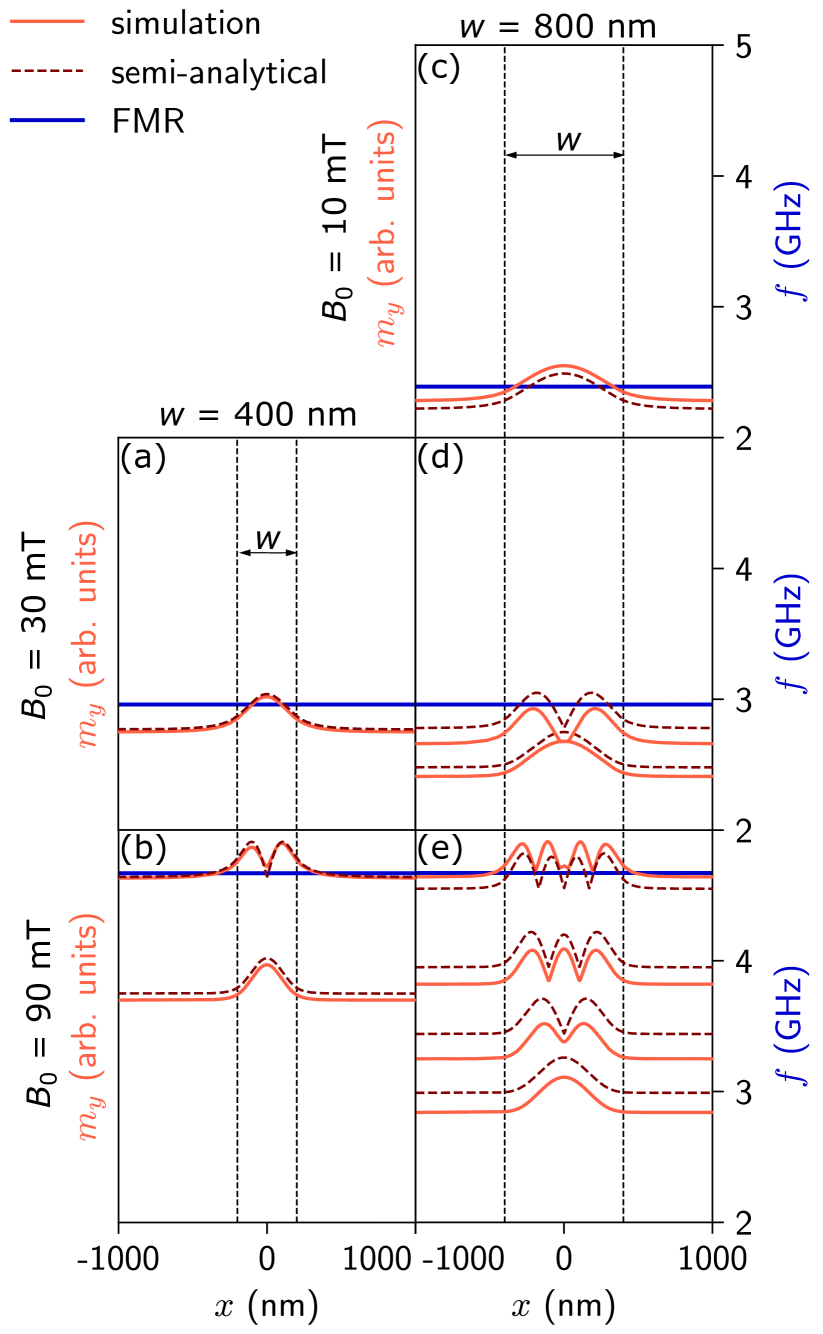
Figure 4: The SW profiles of the modes localized in the effective field well produced by SC strip for the external field values $B_{0}=10$ mT (c), $30$ mT (a,d) and $90$ mT (b,e) obtained from micromagnetic simulations using Mumax3 environment (light red solid lines) and the results of the semi-analytical model (red dashed lines). The blue lines show FMR frequency of a homogenous film for given external magnetic field $B_{0}$ value in the absence of the SC strip. The left and right columns correspond to the SC width $w=400$ nm and $800$ nm, respectively. Vertical black dashed lines indicate the position of the SC strip edges. All the figures share the same frequency and space scales and the amplitude of modes is normalized to enhance the readability of the figure (the difference between the results obtained by the semi-analytical approach and micromagnetic simulations is shown by the offset in the figure).

In Fig. 4(c-e), for $w=800$ nm, we observe a larger number of localized SW modes, what is caused by two factors: (i) the frequency difference between SW mode energy levels becomes smaller due to the widening of the well (the main factor), and (ii) the depth of the well is slightly increased with the widening of SC strip (e.g., for the $w=800$ nm $\Delta B_{sc,y}$ is about 1.4 times larger than for $w=400$ nm). Thus, for $w=800$ nm, there are 1, 2, and 4 localized modes for $B_{0}=10$ mT (Fig.. 4(c)), $30$ mT (Fig. 4(d)), and $90$ mT (Fig. 4(e)), respectively. It should be noted that the approximation of the well $B_{{\rm sc},y}(x)$ by a parabolic well (13) is valid in the considered system only for finite range of the widths $w$ (around $350$ nm), while for much smaller or larger width, the terms higher than quadratic must be included in the expansion (13). For example, for $w=400$ nm and $800$ nm, the approximation of $B_{sc,y}$ requires including up to $4^{\rm th}$ and $6^{\rm th}$ order terms, respectively. The semi-analytical results (dashed lines) are in relatively good agreement with numerical solution of LL equation obtained using the MuMax3 environment (solid lines). Due to the presence of higher order terms in $B_{{\rm sc},y}$, the SW modes are not equidistant in contrast to the eigenfunctions of the quantum harmonic oscillator, i.e., Hermitian functions. However, our mode profiles can be approximated by Hermitian functions with fitting parameter $\beta_{2}$ in (15). This trick allowed us to simplify the averaged demagnetizing field to a compact form (18) (see Appendix B) and easily find the eigenfrequencies (17).

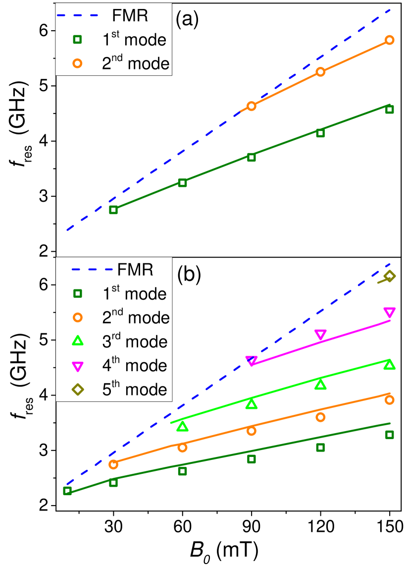
Figure 5: The dependence of the localized SW modes on the external magnetic field $B_{0}$ for the systems with SC strip width $w=400$ nm (a) and $w=800$ nm (b). The solid lines and square dots correspond to the semi-analytical calculations and micromagnetic simulations respectively. Dashed lines show FMR frequency of the uniformly-magnetized film.

The dependence of frequencies of the localized SW modes on the external magnetic field is presented in Fig. 5 for the SC strip width $w=400$ nm (Fig. 5(a)) and $800$ nm (Fig. 5(b)). The results of semi-analytical calculations and micromagnetic simulations are marked by solid lines and dots, respectively. As mentioned in the previous paragraph, the number of localized modes rises with the increase of the external field value and the width of the SC strip. In general, the results of theoretical calculations and micromagnetic simulations are in good agreement. The discrepancies are larger for the strip width $w=800$ nm than for $400$ nm and they increase with increasing external magnetic field. This can be related to the simplifications underlying our theoretical model, according to which we have neglected the tangential component of the field produced by the SC strip $B_{{\rm sc},x}$, which slightly deflects the static magnetization from the normal to the FM layer and forms a non-collinear magnetization structure in the vicinity of the SC strip edges (see Fig. 2(c)). In our model, we have considered the uniform magnetization ground state where the FM layer is magnetized out of plane. This assumption is reasonable because the magnetization deviation angle $\theta_{M}$ is relatively small for a narrow strip, while for a wider strip the deviation angle is larger and increases significantly for large external field values. To prove that this is the main reason for the discrepancies between micromagnetic simulations and the semi-analytical model, we have performed micromagnetic simulations with $B_{{\rm sc},x}=0$, which showed results much closer to theoretical calculations. Small differences can also be caused by the use of the diagonal approximation in our theory. However, the diagonal elements of the dynamical demagnetization field are quite small, which means that non-diagonal elements can really be neglected because they are usually smaller than diagonal elements.

IV Conclusions

We examined a superconductor-ferrimagnet hybrid planar nanostructure wherein a flat SC strip is situated above a uniform FM layer while the external field is applied out of plane. In this configuration, the flat SC strip, being in a Meissner state, produces a stray field that reduces the static effective field inside the thin FM layer placed below. When the FM layer is made of soft magnetic material with PMA, the SW modes can be confined within the region of lowered field (i.e. in the well of internal field). These modes have frequencies lower than the FMR frequency of the FM layer, which explains their exponential decay outside the region of the well. By adjusting the value of the uniform external field, we can control the depth of the well and modify the number and frequencies of confined SW modes. This outcome is difficult to achieve in the conventional magnonic nanostructures where the stray field, as a result of demagnetization, depends on the geometry and magnetic configuration. The first is determined at the fabrication stage and the latter can be modified by an external field, but its full control requires a strong fields due to large demagnetization effects in planar structures.

Our work integrates the numerical and semi-analytical studies. The analytical approach is computationally undemanding and provides deep insight into the magnetization dynamics and the mechanism of SW localization in dipolar-coupled superconductor-ferrimagnet systems. The presented ideas can be used to design superconductor-ferrimagnet hybrid devices for on-demand control of SW localization and propagation.

Data availability

Data supporting this study are openly available from the repository at https://zenodo.org/records/10405886.

Appendix A Dispersion relation – derivation

The dispersion relation can be derived from Eq. (12) after introducing the average of the dipolar field (dipolar operator) in the way similar to the approach known in quantum mechanics. Let us express each SW mode by the function from orthonormal base: $m_{p,n}(x)\approx C_{p}M_{\rm s}\psi_{n}(Kx)$ as in Eq. (15). When we introduce the norm $\langle\psi^{2}_{n}\rangle:=\int_{V}dv|\psi_{n}(Kx)|^{2}\!=\!\frac{ab}{K}$, and then multiply both equations in (12) by $\psi^{*}_{n}(Kx)$ and integrate them over the whole volume of magnetic system, we obtain:

$$\begin{split}\;\;i\omega\;C_{x}\langle\psi^{2}_{n}\rangle&=C_{z}\langle\psi_{n}|\Xi(x)|\psi_{n}\rangle-|\gamma|\mu_{0}\langle h_{{\rm d},z}\rangle_{n},\\ -i\omega\;C_{z}\langle\psi^{2}_{n}\rangle&=C_{x}\langle\psi_{n}|\Xi(x)|\psi_{n}\rangle-|\gamma|\mu_{0}\langle h_{{\rm d},x}\rangle_{n},\end{split}$$ (23)

where $\langle h_{{\rm d},p}\rangle_{n}:=\int_{V}dv\psi^{*}_{n}(Kx)h_{{\rm d},p}(x)$ for $p=\{x,y\}$ can be considered as an averaged component of the dynamic demagnetizing field. This definition is clear when we notice that the field $h_{{\rm d},p,n}$ is the result of action of the integral operator on $\psi_{n}(Kx)$ (strictly related to the magnetization $m_{p,n}(x)$) – see Eq. (16). Taking into account that $\psi_{n}(Kx)$ are eigenfunctions of the operator $\Xi(x)$ with the eigenvalues $\omega_{0,n}$, but not of the dynamical demagnetizing field operator, Eq. (23) can be rewritten as:

$$\begin{split}\;\;i\omega\;C_{x}&=C_{z}\big{(}\omega_{0,n}-|\gamma|\mu_{0}M_{\rm s}\langle\tilde{h}_{{\rm d},z}\rangle_{n}\big{)},\\ -i\omega\;C_{z}&=C_{x}\big{(}\omega_{0,n}-|\gamma|\mu_{0}M_{\rm s}\langle\tilde{h}_{{\rm d},x}\rangle_{n}\big{)},\end{split}$$ (24)

where $\langle\tilde{h}_{{\rm d},p}\rangle_{n}=1/(C_{p}M_{\rm s})\langle h_{{\rm d},p}\rangle$ is a dimensionless averaged field (see Appendix B). The homogeneous set of equations (24) gives non-trivial solution for the resonance frequency $\omega_{n}$ when

$$\begin{split}\begin{vmatrix}\;\;i\omega\;&\omega_{0,n}-|\gamma|\mu_{0}M_{\rm s}\langle\tilde{h}_{{\rm d},z}\rangle_{n}\\ \omega_{0,n}-|\gamma|\mu_{0}M_{\rm s}\langle\tilde{h}_{{\rm d},x}\rangle_{n}&-i\omega\end{vmatrix}=0\end{split},$$ (25)

which leads to dispersion relation shown in Eq. (17).

Appendix B Averaged dipolar field – derivation

For every $n^{\rm th}$ SW mode $\mathbf{m}_{n}(x)$ (confined in the well of stray field), the dynamical demagnetizing field $\mathbf{h}_{{\rm d},n}(x)$ (related to own dynamics of $\mathbf{m}_{n}(x)$) is given by Eq. (16). The field $\mathbf{h}_{{\rm d},n}(x)$ can be considered as a result of action of integral operator on magnetization $\mathbf{m}_{n}$. When we approximate $\mathbf{m}_{n}$ by the function $\psi_{n}(Kx)$ from orthonormal set: $m_{p,n}(x)\approx C_{p}M_{\rm s}\psi_{n}(Kx)$ (see Eq. (15)) and integrate $\mathbf{h}_{{\rm d},n(x)}$ over the whole volume with $\psi_{n}(Kx)$, we obtain average value of the dipolar field operator:

$$\begin{split}\langle h_{{\rm d},p}\rangle_{n}\!=\!-M_{\rm s}\sum_{q}C_{q}\int_{V}\int_{V^{\prime}}\!dvdv^{\prime}\;&\psi_{n}(Kx)\psi_{n}(Kx^{\prime})\times\\ &\frac{d^{2}}{dp\,dq^{\prime}}\frac{1}{4\pi|\mathbf{r}-\mathbf{r^{\prime}}|},\end{split}$$ (26)

where the indices $p$ and $q$ run over the coordinates $x$ and $z$, and derivative $\frac{d}{dq^{\prime}}$ means $\frac{d}{dx^{\prime}}$ (or $\frac{d}{dz^{\prime}}$) for $q=x$ (or $q=z$). Each of the integrals in (26) is actually a three-fold integral: $\int_{-\infty}^{\infty}dx\int_{y_{0}-a/2}^{y_{0}+a/2}dy\int_{-b/2}^{b/2}dz$, where $y_{0}=-(t/2+g+a/2)$. This problem can be simplified when we express the function $\frac{1}{4\pi|\mathbf{r}-\mathbf{r^{\prime}}|}$ in the Fourier space for the wave vector $\mathbf{k}=k_{x}\hat{\mathbf{x}}+k_{z}\hat{\mathbf{z}}$ [39]:

$$\begin{split}\frac{1}{4\pi|\mathbf{r}-\mathbf{r^{\prime}}|}=\frac{1}{2\pi}\!\int_{-\infty}^{\infty}\int_{-\infty}^{\infty}\!dk_{x}dk_{z}\;\frac{1}{k}e^{-k|y-y^{\prime}|}\times\\ e^{ik_{x}(x-x^{\prime})}e^{ik_{z}(z-z^{\prime})},\end{split}$$ (27)

where $k=\sqrt{k_{x}^{2}+k_{y}^{2}}$, and then use the identities:

$$\begin{split}\int_{y_{0}-a/2}^{y_{0}+a/2}\int_{y_{0}-a/2}^{y_{0}+a/2}\!\!dydy^{\prime}\;\frac{1}{k}e^{-k|y-y^{\prime}|}=\frac{2a}{k}\left(\!1-\frac{1-e^{-ka}}{ka}\!\right),\\ \int_{-b/2}^{b/2}\int_{-b/2}^{b/2}\!\!dzdz^{\prime}e^{ik_{z}(z-z^{\prime})}=2\pi b\;\delta(k_{z}),\;{\rm for}\;b\!\rightarrow\!\infty.\end{split}$$ (28)

This allows to express (26) in the form:

$$\begin{split}\langle h_{{\rm d},p}\rangle_{n}\!=\!-M_{\rm s}\frac{ab}{K^{2}}\sum_{q}C_{q}\int dk_{x}\left(\int dk_{z}\frac{k_{p}k_{q}}{k^{2}}\times\right.\\ \left.\left(1-\frac{1-e^{ka}}{ka}\right)\delta(k_{z})\,\tilde{\psi}_{n}^{2}\!\left(\frac{k_{x}}{K}\right)\right).\end{split}$$ (29)

One can notice that $\langle h_{{\rm d},z}\rangle_{n}=0$ and $\langle h_{{\rm d},x}\rangle_{n}$ contains only the term for $p=x$. In the linear regime, the dynamic demagnetizing field scales linearly with the SW amplitude, therefore, it is useful to introduce the normalized dimensionless average field:

$$\langle\tilde{h}_{{\rm d},x}\rangle_{n}=\frac{1}{C_{x}M_{\rm s}}\langle h_{{\rm d},x}\rangle_{n},$$ (30)

where $C_{x}M_{\rm s}$ is a SW amplitude in A/m. Finally, Eqs. (29) and (30) lead to Eq. (18).

See pages 1 of SM_final.pdf See pages 2 of SM_final.pdf See pages 3 of SM_final.pdf

References

- Ran et al. [2019] S. Ran, C. Eckberg, Q.-P. Ding, Y. Furukawa, T. Metz, S. R. Saha, I.-L. Liu, M. Zic, H. Kim, J. Paglione, and N. P. Butch, Nearly ferromagnetic spin-triplet superconductivity, Science 365, 684 (2019).
- Saxena et al. [2000] S. S. Saxena, P. Agarwal, K. Ahilan, F. M. Grosche, R. K. W. Haselwimmer, M. J. Steiner, E. Pugh, I. R. Walker, S. R. Julian, P. Monthoux, G. G. Lonzarich, A. Huxley, I. Sheikin, D. Braithwaite, and J. Flouquet, Superconductivity on the border of itinerant-electron ferromagnetism in UGe2, Nature 406, 587 (2000).
- Sinha et al. [1982] S. Sinha, G. Crabtree, D. Hinks, and H. Mook, Study of coexistence of ferromagnetism and superconductivity in single crystal ErRh4B4, Physica B+C 109-110, 1693 (1982), 16th International Conference on Low Temperature Physics, Part 3.
- Bernhard et al. [1999] C. Bernhard, J. L. Tallon, C. Niedermayer, T. Blasius, A. Golnik, E. Brücher, R. K. Kremer, D. R. Noakes, C. E. Stronach, and E. J. Ansaldo, Coexistence of ferromagnetism and superconductivity in the hybrid ruthenate-cuprate compound studied by muon spin rotation and dc magnetization, Phys. Rev. B 59, 14099 (1999).
- Lyuksyutov and Pokrovsky [2005] I. F. Lyuksyutov and V. L. Pokrovsky, Ferromagnet–superconductor hybrids, Adv. Phys. 54, 67 (2005).
- Linder and Robinson [2015] J. Linder and J. W. A. Robinson, Superconducting spintronics, Nat. Phys. 11, 307 (2015).
- Bespalov [2022] A. Bespalov, Electromagnetic proximity effect in superconductor/ferromagnet bilayers with in-plane magnetic texture, Phys. C: Supercond. 595, 1354032 (2022).
- Cai et al. [2023] R. Cai, I. Žutić, and W. Han, Superconductor/ferromagnet heterostructures: A platform for superconducting spintronics and quantum computation, Adv. Quantum Technol. 6, 2200080 (2023).
- Bergeret et al. [2001] F. S. Bergeret, A. F. Volkov, and K. B. Efetov, Long-range proximity effects in superconductor-ferromagnet structures, Phys. Rev. Lett. 86, 4096 (2001).
- Genenko et al. [1999] Y. A. Genenko, A. Usoskin, and H. C. Freyhardt, Large predicted self-field critical current enhancements in superconducting strips using magnetic screens, Phys. Rev. Lett. 83, 3045 (1999).
- Milošević et al. [2005] M. V. Milošević, G. R. Berdiyorov, and F. M. Peeters, Mesoscopic field and current compensator based on a hybrid superconductor-ferromagnet structure, Phys. Rev. Lett. 95, 147004 (2005).
- Vlasko-Vlasov et al. [2017] V. K. Vlasko-Vlasov, F. Colauto, A. I. Buzdin, D. Rosenmann, T. Benseman, and W.-K. Kwok, Magnetic gates and guides for superconducting vortices, Phys. Rev. B 95, 144504 (2017).
- Golovchanskiy et al. [2018] I. A. Golovchanskiy, N. N. Abramov, V. S. Stolyarov, V. V. Bolginov, V. V. Ryazanov, A. A. Golubov, and A. V. Ustinov, Ferromagnet/superconductor hybridization for magnonic applications, Adv. Funct. Mater. 28, 1802375 (2018).
- Golovchanskiy et al. [2019] I. A. Golovchanskiy, N. N. Abramov, V. S. Stolyarov, P. S. Dzhumaev, O. V. Emelyanova, A. A. Golubov, V. V. Ryazanov, and A. V. Ustinov, Ferromagnet/superconductor hybrid magnonic metamaterials, Adv. Sci. 6, 1900435 (2019).
- Golovchanskiy et al. [2020] I. A. Golovchanskiy, N. N. Abramov, V. S. Stolyarov, A. A. Golubov, V. V. Ryazanov, and A. V. Ustinov, Nonlinear spin waves in ferromagnetic/superconductor hybrids, J. Appl. Phys. 127, 093903 (2020).
- Dobrovolskiy et al. [2019] O. V. Dobrovolskiy, R. Sachser, T. Brächer, T. Böttcher, V. V. Kruglyak, R. V. Vovk, V. A. Shklovskij, M. Huth, B. Hillebrands, and A. V. Chumak, Magnon–fluxon interaction in a ferromagnet/superconductor heterostructure, Nat. Phys. 15, 477 (2019).
- Niedzielski et al. [2023] B. Niedzielski, C. Jia, and J. Berakdar, Magnon-fluxon interaction in coupled superconductor/ferromagnet hybrid periodic structures, Phys. Rev. Appl. 19, 024073 (2023).
- Shekhter et al. [2011] A. Shekhter, L. N. Bulaevskii, and C. D. Batista, Vortex viscosity in magnetic superconductors due to radiation of spin waves, Phys. Rev. Lett. 106, 037001 (2011).
- Dobrovolskiy and Chumak [2022] O. V. Dobrovolskiy and A. V. Chumak, Nonreciprocal magnon fluxonics upon ferromagnet/superconductor hybrids, J. Magn. Magn. Mater. 543, 168633 (2022).
- Dobrovolskiy et al. [2023] O. V. Dobrovolskiy, Q. Wang, D. Y. Vodolazov, B. Budinska, S. Knauer, R. Sachser, M. Huth, and A. I. Buzdin, Cherenkov radiation of spin waves by ultra-fast moving magnetic flux quanta (2023), arXiv:2103.10156 [cond-mat.other] .
- Schmidt [1997] V. V. Schmidt, The physics of superconductors: Introduction to fundamentals and applications (Springer Verlag, Berlin-Heidelberg-New York, 1997).
- Fiolhais and Essén [2014] M. C. Fiolhais and H. Essén, Magnetic field expulsion from an infinite cylindrical superconductor, Phys. C: Supercond. 497, 54 (2014).
- Badía and Freyhardt [1998] A. Badía and H. C. Freyhardt, Meissner state properties of a superconducting disk in a non-uniform magnetic field, J. Appl. Phys. 83, 2681 (1998).
- Brandt [1994a] E. H. Brandt, Thin superconductors in a perpendicular magnetic ac field: General formulation and strip geometry, Phys. Rev. B 49, 9024 (1994a).
- Brandt [1994b] E. H. Brandt, Thin superconductors in a perpendicular magnetic ac field. II. Circular disk, Phys. Rev. B 50, 4034 (1994b).
- Gurevich and Melkov [1996] A. Gurevich and G. Melkov, Magnetization oscillations and waves (CRC Press, London, 1996).
- Kakazei et al. [2004] G. N. Kakazei, P. E. Wigen, K. Y. Guslienko, V. Novosad, A. N. Slavin, V. O. Golub, N. A. Lesnik, and Y. Otani, Spin-wave spectra of perpendicularly magnetized circular submicron dot arrays, Appl. Phys. Lett. 85, 443 (2004).
- Kakazei et al. [2012] G. N. Kakazei, G. R. Aranda, S. A. Bunyaev, V. O. Golub, E. V. Tartakovskaya, A. V. Chumak, A. A. Serga, B. Hillebrands, and K. Y. Guslienko, Probing dynamical magnetization pinning in circular dots as a function of the external magnetic field orientation, Phys. Rev. B 86, 054419 (2012).
- Bunyaev et al. [2015] S. A. Bunyaev, V. O. Golub, O. Y. Salyuk, E. V. Tartakovskaya, N. M. Santos, A. A. Timopheev, N. A. Sobolev, A. A. Serga, A. V. Chumak, B. Hillebrands, and G. N. Kakazei, Splitting of standing spin-wave modes in circular submicron ferromagnetic dot under axial symmetry violation, Sci. Rep. 5, 18480 (2015).
- Klein et al. [2008] O. Klein, G. de Loubens, V. V. Naletov, F. Boust, T. Guillet, H. Hurdequint, A. Leksikov, A. N. Slavin, V. S. Tiberkevich, and N. Vukadinovic, Ferromagnetic resonance force spectroscopy of individual submicron-size samples, Phys. Rev. B 78, 144410 (2008).
- Tartakovskaya et al. [2016] E. V. Tartakovskaya, M. Pardavi-Horvath, and R. D. McMichael, Spin-wave localization in tangentially magnetized films, Phys. Rev. B 93, 214436 (2016).
- Kharlan et al. [2019] J. Kharlan, P. Bondarenko, M. Krawczyk, O. Salyuk, E. Tartakovskaya, A. Trzaskowska, and V. Golub, Standing spin waves in perpendicularly magnetized triangular dots, Phys. Rev. B 100, 184416 (2019).
- Kalinikos and Slavin [1986] B. A. Kalinikos and A. N. Slavin, Theory of dipole-exchange spin wave spectrum for ferromagnetic films with mixed exchange boundary conditions, J. Phys. Condens. Matter 19, 7013 (1986).
- Vansteenkiste et al. [2014] A. Vansteenkiste, J. Leliaert, M. Dvornik, M. Helsen, F. Garcia-Sanchez, and B. Van Waeyenberge, The design and verification of MuMax3, AIP Adv. 4, 107133 (2014).
- Gubin et al. [2005] A. I. Gubin, K. S. Il’in, S. A. Vitusevich, M. Siegel, and N. Klein, Dependence of magnetic penetration depth on the thickness of superconducting Nb thin films, Phys. Rev. B 72, 064503 (2005).
- Böttcher et al. [2022] T. Böttcher, M. Ruhwede, K. Levchenko, Q. Wang, H. Chumak, M. Popov, I. Zavislyak, C. Dubs, O. Surzhenko, B. Hillebrands, A. Chumak, and P. Pirro, Fast long-wavelength exchange spin waves in partially compensated Ga:YIG, Appl. Phys. Lett. 120, 102401 (2022).
- McConville and Serin [1965] T. McConville and B. Serin, Ginzburg-Landau Parameters of Type-II Superconductors, Phys. Rev. 140, A1169 (1965).
- Williamson [1970] S. J. Williamson, Bulk upper critical field of clean type-II superconductors: V and Nb, Phys. Rev. B 2, 3545 (1970).
- Guslienko and Slavin [2011] K. Y. Guslienko and A. N. Slavin, Magnetostatic Green’s functions for the description of spin waves in finite rectangular magnetic dots and stripes, J. Magn. Magn. Mater. 323, 2418 (2011).