Fracture process of composite material in a spring network model

Abstract

We analyze a two-dimensional spring network model comprising breakable and unbreakable springs. Computer simulations showed this system to exhibit intermittent stress drops in a larger strain regime, and these stress drops resulted in ductile-like behavior. The scaling analysis reveals that the avalanche size distribution demonstrates a cut-off, depending on its internal structure. This study also investigates the relationship between cluster growth and stress drop, and we show that the amount of stress drop increases in terms of power law, corresponding to crack growth. The crack length distribution also demonstrates a cut-off depending on its internal structure. The results show that both the cluster growth-stress drop relationship and the crack size distribution are scaled by the quantity related to the internal structure, and the relevance of the exponent that scales the cluster growth-stress drop relationship to the exponent that scales crack size distribution is verified.

I Introduction

Fracture is one of the most familiar nonequilibrium phenomena and has attracted interest from not only engineering but also fundamental science. Recently, studies have shown that fracture in disordered media has many interesting aspects such as the power law of released-energy statistics[1, 2, 3, 4], the self-affine nature of crack morphology[5, 6, 7], intermittent dynamics[3, 8], and pattern formation[9]. Several studies have focused on understanding these properties by using models, such as the fiber bundle model[10], fuse model[11], and spring model[12].

Further, because of their internal structure, composite materials are known to display different fracture properties than those of normal disordered materials. An example of composite materials is fiber-reinforced ceramics, a composite of ceramics, which is a typical disordered brittle material, and fiber. Fiber-reinforced ceramics demonstrate greater strength than that of ordinary ceramics and show ductile fractures[13, 14]. In addition to artificial composite materials, there also exist natural composite materials. For example, Nacre is a composite material with organic parts and mineral parts arranged in a layered manner; It shows better fracture strength because of this internal structure[15, 16, 17]. This implies that the possibility of fracture processes is determined not entirely by the properties of individual materials but also by the internal structure of the composite material. Then, the following questions arise: What is the difference between the fracture processes of disordered and composite materials with respect to their internal structures? How does the internal structure of a material influence its fracture properties?

To answer these questions, we modeled a composite material with an internal structure of a spring network (SN) model[11], a stochastic fracture model, and simulated its quasi-static tensile fracture mechanism. Our model comprises two spring types: One spring breaks with the application of a specific amount of load and the other is unbreakable under any load. Kun et al. analyzed the fracture of a random mixture of weak and strong fiber composites by using an equal-load sharing and local-load sharing fiber bundle models[18, 19]. Tauber et al.[20] considered a spring model that mimics polymer composites. Compared to their models, we used strong springs in our SN model to form a regular matrix structure. The contributions of this study in terms of determining the effect of the internal structure of composite materials are threefold. First, the present system demonstrates ductile fractures because of its internal structure. Second, the burst size distribution of the present model shows power-law behavior in the intermediate size scale, and it shows cut-off in the case of the larger avalanche. The scaling analysis showed that the burst size distribution can be scaled according to the size scale determined by its internal structure. Finally, the crack size distribution is scaled by the internal-structure-based crack length, and the stress drop caused by crack growth is scaled by the crack-opening length depending on the internal structure of the material. Our model boasts simplicity in capturing the fundamental properties of the fracture process in the composite material with a matrix structure. Moreover, the model can be used as a prototype for composite materials with a more complex internal structure.

The organization of this paper is as follows. In Sec. II, the details of the model and simulation method are presented. Results are described in Sec. III, and conclusions are summarized in Sec. IV.

II Model and simulation

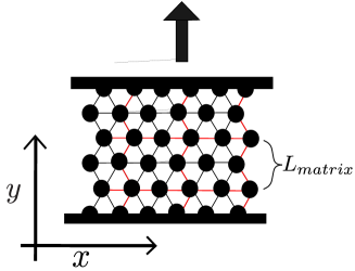
Figure 1: Schematic of the spring network model. $N\times N$ particles are located on a triangular lattice, and nearest-neighbor particles are connected using springs. The black bonds correspond to breakable springs and the red bond corresponds to unbreakable springs. Unbreakable springs are regularly distributed spatially to constitute a $L_{matrix}\times L_{matrix}$ with an almost square frame. A periodic boundary condition is imposed in the $x$ direction, and a fixed boundary condition is imposed in the $y$ direction for tensile loading.

In this study, we analyzed a two-dimensional SN model, which represents the composite material as a network of particles connected by Hookean springs. The system comprises $N\times N$ particles on a triangular lattice, as shown in Fig. 1. All particles possess the same mass, which is taken to be a mass unit, and each pair of nearest-neighbor particles is connected by the Hookean spring, the natural length of which is represented by lattice spacing $l_{0}$, which is the unit of length. The periodic boundary condition was imposed in the $x$ direction and the fixed boundary condition was imposed in the $y$ direction for tensile loading. Each spring has a fracture threshold of $l^{*}$, which was randomly selected from a uniform distribution between 0 and 1. When the strain of the spring, i.e., $\left\lvert l-l_{0}\right\rvert/l_{0}$, becomes larger than the threshold, $l^{*}$, the spring breaks, and it is removed from the system. In this system, the strains caused by the broken springs were distributed among the remaining live springs to reach the mechanical equilibrium. The successive breaking of many springs is possible, a phenomenon, which hereafter, is referred to as burst or avalanche. The potential energy of this model can be formulated as[21]

$$V=\frac{k}{2}\sum_{\langle i,j\rangle}(|\bm{r_{i}}-\bm{r_{j}}|-l_{0})^{2}g_{ij},$$ (1)

where $\bm{r_{i}}$ is the position vector of the $i$-th particle, $g_{ij}=1$ indicates a live bond, and $g_{ij}=0$ indicates a broken bond. The summing pair $\langle i,j\rangle$ runs the nearest-neighbor pairs on the triangular lattice. Parameter $k$ is a spring constant, taken as unity.

We replaced some springs with unbreakable springs, $l^{*}=\infty$, for modeling the composite material. These unbreakable springs were regularly distributed spatially to constitute a $L_{matrix}\times L_{matrix}$ with an almost square frame. We call this system as the “matrix-mixture system,” and we term the system without unbreakable bonds as the “normal system.” In this study, we take $N=96$ and $L_{matrix}=6,8,12$.

Next, the system was simulated under strain control as follows. The lowest row of particles was fixed, and a small amount of displacement was implemented among the highest row of particles. The system was then allowed to relax to a mechanical equilibrium state. The equilibrium state was explored using the FIRE algorithm[22]. After the system relaxed to the mechanical equilibrium state, we decided on which bonds to break. If a certain spring’s strain was over the fracture threshold, that spring was removed from the system. After removing the springs, the mechanical equilibrium configuration was analyzed again without moving the top particles. This loop was continued until the springs stopped breaking in the mechanical equilibrium state. When the system reached this state, we repeated the same procedure. The simulation was finally stopped when the system completely broke into two pieces or the strain of the system reached $1$. For one small uniaxial extension step, the strain of the system increased by $0.1\%$, i.e., $\Delta\epsilon=0.0001$. Here, the statistically independent 1000 configurations were simulated.

III Result

III.1 Mechanical property

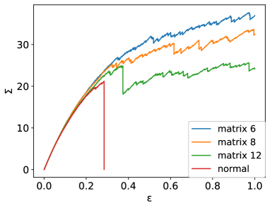
Figure 2: Typical stress-strain response of the system. Every system shows a linear response in a small strain regime. Then, the normal system breaks in a brittle manner. The matrix-mixture systems do not demonstrate such an abrupt change but show ductile-like failures with intermittent stress drops. The size distributions of stress drops vary in each system. As the matrix size of the system increases, the larger stress drop also increases, as shown in Fig. 3.

We first discuss the stress-strain curve of the system. In this study, we compute

$$\Sigma=\frac{k}{H_{0}}\sum_{\langle i,j\rangle}(|\bm{r}_{i}-\bm{r}_{j}|-l_{0})\frac{|y_{j}-y_{i}|}{|\bm{r}_{i}-\bm{r}_{j}|}g_{ij},$$ (2)

as the stress [21], where $H_{0}=Nl_{0}$ is the width of the system. Figure 2 shows the typical stress-strain curve of this system. At the beginning of tension application, all systems follow linear elasticity. After that, the slope of the stress-strain curve reduces because of the increase in damage. Eventually, the normal and matrix-mixture systems show completely different mechanical responses. The normal system shows an abrupt stress drop. As shown in previous studies[11, 23], this stress drop causes the cracks to propagate from one end to another, and the system breaks in two. That is, the normal system shows a brittle fracture. The matrix-mixture systems show similar behavior in the elastic regime as the normal system. However, these systems behave as a ductile material in the larger strain regime. This ductile behavior could be attributed to the intermittent and instantaneous stress changes. Hereafter, we term this stress change as a stress drop, and its magnitude is denoted as $\Delta\Sigma$. The ductile regime frequently displays small-scale stress drops, which cancel out the increase in stress. The comparison of each $L_{matrix}$ shows that the system with a small $L_{matrix}$ value shows less stress drop than the system with a large $L_{matrix}$ value. To quantify this difference, we investigated the distribution of stress drop, $\Delta\Sigma$, which is denoted as $P(\Delta\Sigma)$, as shown in Fig. 3. All negative instantaneous changes in stress were considered. In the smaller stress drop regime, distribution $P(\Delta\Sigma)$ showed power-law decay, and its exponent is almost the same for the different matrix sizes, $L_{matrix}$. In the much larger $\Delta\Sigma$ region, the cut-off was observed to depend on $L_{matrix}$. The result in Fig. 3 suggests that a smaller matrix significantly suppresses large stress drops.

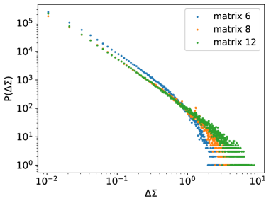
Figure 3: Distribution of stress drop, $P(\Delta\Sigma)$. In the smaller $\Delta\Sigma$ regime, $P(\Delta\Sigma)$ shows power-law decay. The larger $\Delta\Sigma$ regime demonstrates a cut-off, depending on $L_{matrix}$. The distribution is considered by the binning with $1/N$.

III.2 Avalanche

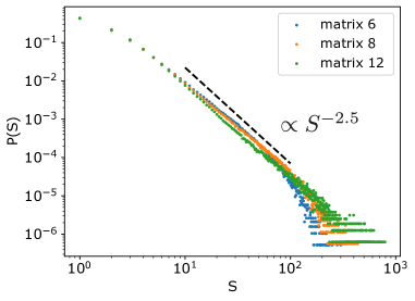
Figure 4: Avalanche size distribution. The black dashed line corresponds to the distribution of the normal SN model, $P(S)\sim S^{-2.5}$.

To understand the effect of suppressing the stress drop by using a matrix structure, we studied the difference between the burst size distribution $P(S)$ between the normal and matrix-mixture SN models, where $S$ is the number of breaking springs during the single loading step with respect to $\Delta\epsilon$. In the normal SN model, the burst size distribution, $P(S)$, behaves as $\sim S^{-\tau}$, and exponent $\tau$=2.5[11]. We plot the burst size distribution in Fig. 4, wherein all burst events are considered. First, as shown, exponent $\tau$ decreases with the consideration of the internal structure in the matrix-mixture system. This indicates that smaller bursts are more likely to occur in the smaller matrix-mixture system. Second, Figure 4 shows that the burst size distribution demonstrates a cut-off size depending on its matrix size. Based on these observations, the matrix structure increases the burst events until the intermediate scale and suppresses burst events on a larger scale.

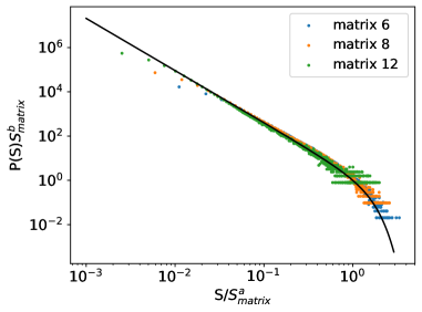
Figure 5: Scaled avalanche size distribution. The solid line corresponds to the fitting function, $f(x)=x^{-\tau}\operatorname{erfc}(x-1)$, with respect to the scaling hypothesis shown in Eq. (3). Here, we take scaling variables as $a=1.0$, $b=2.38$, and $\tau=2.35$.

Next, by using scaling analysis, we discuss the differences among each matrix-mixture system in terms of the burst size distribution. We assume that the burst size distribution has the following scaling form with exponents $a$ and $b$:

$$P(S,L_{matrix})=S_{matrix}^{-b}f(S/S^{a}_{matrix}),$$ (3)

where $S_{matrix}$ is the number of breakable springs in the matrix calculated as $S_{matrix}=3L_{matrix}(L_{matrix}-1)$, and $f(x)$ is the scaling function[19]. The result of the scaling analysis showed that the distribution of burst size, $P(S)$, collapses onto the master curve. We achieved a favorable conformance between the data and master curve $f(x)$, formulated as $f(x)=x^{-\tau}\operatorname{erfc}(x-a)$ with $a=1.0$, $b=2.38$, and $\tau=2.35$. This result indicates that the burst event follows the power law with the same exponent, $\tau=2.35$, until the burst size was less than $S_{matrix}$ and showed sigmoidal decay once it increased more than $S_{matrix}$. The functional form of $f(x)$ indicates that any apparent change in $\tau$ and the decay behavior in Fig. 5 can be attributed to the difference in $S_{matrix}$. These results show that the stress drops were suppressed by the matrix structure because the fracture events were suppressed by the cut-off size, $S_{matrix}$.

III.3 Crack coalescence and stress drop

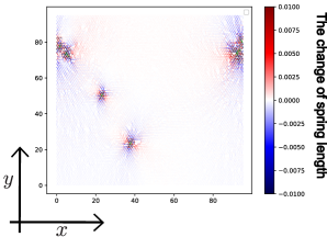
(a) Elastic regime ($\epsilon=0.153,\Delta\Sigma=0.02$)

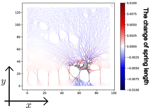
(b) Ductile regime ($\epsilon=0.5615,\Delta\Sigma=0.11$)

Figure 6: Snapshots after breaking events in elastic and ductile regimes for $L_{matrix}=12$. Springs with reduced (increased) stress compared to those in the previous step are indicated in blue (red), respectively. Broken springs in the previous step are indicated in green. In both snapshots, the number of breaking springs in the previous step is the same, i.e., 10. The left panel shows a smaller stress drop, which is attributed to the burst events occurring at spatially isolated locations. In the right panel, the stress drop is approximately five times larger than in the left panel, and this could be attributed to the fracture events occurring in spatially close locations, accompanied by larger crack growth.

A stress drop depends on not only the number of avalanches but also the spatial distribution of crack formation. Figure 6 illustrates the effect of crack coalescence on stress drops. The figure clearly shows the difference between the spatial distributions of appeared cracks of the elastic and ductile regimes. We could clarify the effects of spatial distribution on the stress drop by observing the internal states of the springs. Figure 6 shows the configuration of the SN model at a certain strain rate. The colors represent the changes in the spring length compared with a previous state, i.e., red corresponds to extended springs and blue corresponds to shrunken springs. In addition, green represents the springs broken in the previous step. In both pictures, the number of breaking springs caused by the single tiny displacement is $10$. In the elastic regime (Fig. 6(a)), each appeared crack was spatially isolated. As such, the rupture of springs does not significantly affect the entire structure. On the contrary, as the fracturing proceeds to the ductile regime (Fig. 6(b)), the breaking of springs tends to show a more significant effect on the internal structure by coalescing with existing cracks.

This result suggests that the amount of crack growth is essential for how stress is reduced in certain fracture events[24]. Thus, we quantitatively analyzed the relationship between crack growth and stress drop.

Figure 7: Schematic of the definition of the cluster size of cracks. The black, green, and red lines correspond to breakable, broken, and unbreakable springs, respectively. The single crack cluster does not extend over the unbreakable bond. Thus, in this case, there are two clusters: $N_{C=3}=1$ and $N_{C=6}=1$.

Figure 8: Relationship between the amount of crack growth, $\Delta C$, and the amount of stress drop, $\Delta\Sigma$, in terms of matrix size. Inset: Bare relation. All matrix sizes in the smaller $\Delta C\lesssim 10^{1}$ regime display the same behavior, which deviates in the larger $\Delta C$ regime. Main: Scaled relation. This deviation can be scaled with respect to $\Delta C$ divided by $L_{matrix}^{\zeta}$, where the exponent is $\zeta=0.55$. For plotting, the horizontal axis, $\Delta C$, has been binned by an integer to reduce fluctuations.

To quantify the effect of crack growth, we introduced two quantities, $C$ and $N_{C}(\epsilon)$, where $C$ corresponds to the size of the crack cluster and $N_{C}(\epsilon)$ is the number of crack clusters with size $C$ at strain $\epsilon$, as shown in Fig. 7. In this study, we assumed that the single crack cluster does not extend over the unbreakable bond. If the cluster seems to extend over the unbreakable bond, we have identified it as two separate clusters.

Based on the percolation theory[25], the increment in crack cluster size, $\Delta C$, according to the amount of crack growth is defined as

$$\Delta C=\sqrt{\sum_{C}\left(C^{2}N_{C}(\epsilon)-C^{2}N_{C}(\epsilon-\Delta\epsilon)\right)}.$$ (4)

This quantity generates a large value for the large clusters of broken springs, even for the same number of broken springs. The inset of Fig. 8 shows the stress drop as a function of $\Delta C$. The amount of stress drops roughly increases in a power-law manner. The inset of Fig. 8 shows the behavior of the stress drop to deviate near $\Delta C\sim 10^{1}$. This deviation can be scaled with respect to $\Delta C$ over $L_{matrix}^{\zeta}$, as shown in Fig. 8. Exponent $\zeta\simeq 0.55$ results in the best fit in regime $\Delta C>30$.

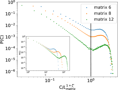
Figure 9: Crack size distribution for each matrix size at the final state, $\epsilon=1$. Inset: Bare distribution. This distribution follows the power law in small-sized cracks. A cut-off size corresponding to its matrix size is observed in the large-sized cracks. Main: Scaled distribution. By scaling the crack size with respect to $L^{1+\zeta^{\prime}}_{matrix}$, we get the point at which deviation from the power law begins and the cut-off size can be scaled independently on the matrix size. Exponent $\zeta^{\prime}=0.56$ is almost the same as $\zeta$ in Fig. 8 The black dashed line corresponds to $C/L_{matrix}^{1+\zeta^{\prime}}=1$.

Finally, we analyzed the crack size distribution, $P(C)$, for each matrix at the final state, $\epsilon=1$. In the inset of Fig. 9, the distribution shows the power-law decay in the small crack length regime. This decay is consistent with that observed in previous studies[26]. In this regime, the matrix structure does not affect the crack size. The effect of matrix structure becomes apparent in the region with large cracks. The distribution shows a cut-off corresponding to the matrix size for a long crack. This result clearly shows that the matrix structure of the system suppresses crack growth. By scaling the crack size by using $L^{1+\zeta^{\prime}}_{matrix}$, the point at which deviation from the power law begins and the cut-off size can be scaled independently on the matrix size is shown in Fig. 9. We achieved the best fit by using exponent $\zeta^{\prime}=0.56$, and this is almost the same as $\zeta$ in Fig. 8. We ascribe this agreement between $\zeta$ and $\zeta^{\prime}$ to corresponding $L_{matrix}^{\zeta}$ with an effective crack width. Previous research[27] showed that the roughness exponent of the random fuse model was $2/3$, and it was $0.62$ for the Born model[28]; These values are close to the value achieved in the current study: $\zeta\ \simeq 0.55$. Considering $L_{matrix}^{\zeta^{\prime}}$ as the characteristic length of the crack width in the matrix, $L_{matrix}^{1+\zeta^{\prime}}$ can be identified according to the typical crack length in the matrix. The crack length distribution follows a power law similar to that of the normal SN model for small crack lengths. However, owing to the matrix structure, the cracks cannot grow larger, and a peak appears in the distribution after the scale of $L_{matrix}^{1+\zeta^{\prime}}$.

IV Conclusion

In this study, we analyzed the fracture process of composite materials and their statistical properties according to the internal structure of the material by using the SN model with a mixture of breakable and unbreakable springs. We found that the proposed SN model shows ductile-like fractures because of intermittent stress drops. In addition, we revealed that avalanche size distribution is well scaled by the number of springs in matrix $L_{matrix}(3L_{matrix}-1)$. The scaling function can be written as $x^{-\tau}\operatorname{erfc}(x-1)$, suggesting that the fracture event follows the power law, similar to the normal SN model[11], and it decays abruptly when reaching a specific number of springs in a matrix. We also revealed the relationship between crack cluster growth and stress drop. Larger clusters appeared when cracks merged, resulting in a more significant stress drop. On average, the amount of stress drop increased based on the power law, followed by the growth in crack clusters. The cluster size distribution showed a cut-off corresponding to the matrix size, and the size cut-off could be rescaled by a typical crack length in the matrix. The matrix size limits the size of the cluster. Our simple model can capture macroscopic fracture characteristics of broad brittle material composites such as fiber-reinforced ceramics. Although we limited the distribution of unbreakable springs to a square matrix, the distribution of strong springs is presumed to affect the fracture process. Therefore, another type of distribution, such as random distribution, must be tested in future works.