MS-0000-0000.00

Dai et al.

Learning Merton’s Strategies in an Incomplete Market

Learning Merton’s Strategies in an Incomplete Market: Recursive Entropy Regularization and Biased Gaussian Exploration

Min Dai Department of Applied Mathematics and School of Accounting and Finance, The Hong Kong Polytechnic University, Hung Hom, Hong Kong, Kowloon, mindai@polyu.edu.hk Yuchao Dong Key Laboratory of Intelligent Computing and Applications (Tongji University), Ministry of Education and School of Mathematical Sciences, Tongji University, Shanghai, China, Shanghai 200092, ycdong@tongji.edu.cn Yanwei Jia Department of Systems Engineering and Engineering Management, The Chinese University of Hong Kong, Shatin, Hong Kong, New Territories, yanweijia@cuhk.edu.hk Xun Yu Zhou Department of Industrial Engineering and Operations Research & Data Science Institute, Columbia University, New York, USA, NY 10027, xz2574@columbia.edu

We study Merton’s expected utility maximization problem in an incomplete market, characterized by a factor process in addition to the stock price process, where all the model primitives are unknown. We take the reinforcement learning (RL) approach to learn optimal portfolio policies directly by exploring the unknown market, without attempting to estimate the model parameters. Based on the entropy-regularization framework for general continuous-time RL formulated in Wang et al. (2020), we propose a recursive weighting scheme on exploration that endogenously discounts the current exploration reward by past accumulative amount of exploration. Such a recursive regularization restores the optimality of Gaussian exploration. However, contrary to the existing results, the optimal Gaussian policy turns out to be biased in general, due to the interwinding needs for hedging and for exploration. We present an asymptotic analysis of the resulting errors to show how the level of exploration affects the learned policies. Furthermore, we establish a policy improvement theorem and design several RL algorithms to learn Merton’s optimal strategies. At last, we carry out both simulation and empirical studies with a stochastic volatility environment to demonstrate the efficiency and robustness of the RL algorithms in comparison to the conventional plug-in method.

Reinforcement learning; Merton’s problem; incomplete market; recursive utility; entropy regularization; Gaussian exploration; biased stochastic policy

1 Introduction

Merton’s expected utility maximization model (Merton, 1969) and its subsequent rich variants are central to continuous-time finance. The traditional paradigm for applying the Merton models to practice follows the so-called “separation principle” (separation between estimation and optimization), also known as the “plug-in” method. Starting from a basic stock price model – be it the simplest Black–Scholes, a stochastic volatility model, or a Lèvy process – an econometrician estimates the model parameters/primitives from historical data using statistical or machine learning methods and then passes on to an (optimization) theorist. The latter plugs in the estimated values to the resulting stochastic control problem and solves it (rarely) analytically or (commonly) numerically via solving Pontryagin’s maximum principle conditions or Hamilton–Jacobi–Bellman (HJB) partial differential equations (PDEs). The endeavors of the econometrician and the theorist are thus separated: The former deals with estimation only, and the latter takes the estimated model as given and focuses on optimization. Had an infinite amount of data been available, this division of labor might work – suitable statistical/econometric methods ensure that a reasonable correctness of the model can be validated and the primitives be estimated to the highest accuracy possible. However, in the context of financial markets and asset returns, it has been well documented that accurate estimates of certain parameters – predominantly the expected return – require an amount of data far beyond the history of financial markets (Merton, 1980; Luenberger, 1998). Even worse, a market is most likely non-stationary, defeating the stationarity assumption usually required by those econometric methods. Furthermore, Merton’s strategies, if computable, are typically very sensitive to model primitives. As a result, estimation errors may be significantly amplified rendering the theorist’s results irrelevant to practice.

The drawbacks of the classical plug-in approach are significant and manifested in many dynamic optimization problems beyond financial portfolio choice. The modern reinforcement learning (RL) paradigm takes a conceptually and fundamentally different approach. It still begins with a basic structural model underlying the data-generating process, but it does not assume the model parameters to be given and known, nor does it attempt to estimate them. Instead, RL tries to learn optimal policies or strategies directly, via first parameterizing a policy and then updating (learning) its parameters iteratively to improve the policy until optimality or near-optimality is achieved. The approach accomplishes this typically in three steps: 1) strategically exploring the unknown environment (e.g., a market) by trial-and-error: randomly experimenting different policies according to some carefully designed probability distribution (called a stochastic policy) and observing the responses (called reward or reinforcement signals) from the environment; 2) learning the value function of that stochastic policy based on the reward signals; and 3) improving the stochastic policy based on the learned value function. These steps are called respectively exploration, policy evaluation, and policy improvement, and the resulting algorithms are referred to as the actor (policy)–critic (value function) type in RL. So RL is end-to-end: It maps data to decision policies skipping the middle step of estimating model primitives, guided by the objective to balance exploration (learning) and exploitation (optimization), which are now entangled and engaged simultaneously (rather than separately).

RL has been studied extensively for discrete-time Markov decision processes (MDPs); see, e.g., Sutton and Barto (2011) for a systematic account. But RL or indeed machine learning algorithms in general have often been criticized for lacking a rigorous theoretical ground and hence lacking explainability or interpretability. In recent years, there has been an upsurge of interest in continuous-time RL with continuous state and action spaces, not only because many practical problems are continuous time by nature (e.g. autonomous driving, robot navigation and ultra-high-frequency trading) but also because more analytical tools are available in the continuous setting for developing a rigorous theory. Wang et al. (2020) are the first to formulate continuous-time RL as entropy-regularized relaxed stochastic control problems and prove that the Gibbs measure is the best sampler for exploration. Moreover, the Gibbs measure specializes to Gaussian in the linear–quadratic (LQ) case. Jia and Zhou (2022a, b, 2023) build on this framework to develop rigorous theories for policy evaluation, policy gradient, and q-learning, respectively. A central underpinning of this series of research is the martingality: the learning/updating of the parameters of both the actor and the critic is guided by maintaining the martingality for various stochastic processes. Applications of these general results include, to name just a few, Wang and Zhou (2020) for continuous-time mean–variance pre-committed portfolio choice which is essentially an LQ control problem, Guo et al. (2022) for LQ mean-field games, and Dai et al. (2023) for mean–variance equilibrium policies.

The above continuous-time research adds the entropy of a stochastic policy to the objective function to encourage exploration, with a weighting parameter on the entropy (called the temperature parameter) to explicitly capture the trade-off between exploration and exploitation. There are, however, two issues in the existing research for general continuous-time RL. First, the temperature parameter is taken as an exogenous constant, with little explanation about its choice. Moreover, it is problematic to keep it as a constant throughout because, intuitively, the longer one has explored the environment the less exploration is needed in the future. Second, while Gibbs measure has been derived and the corresponding HJB equation explicitly written for general nonlinear problems, analytical forms of optimal stochastic policies and value functions are so far limited only to the LQ case. Note that explicit expressions facilitate simple parameterizations of policies and value functions, leading to more efficient and computationally less costly RL algorithms than using somewhat brute-force neural networks.

While mean–variance portfolio optimization, originally proposed by Markowitz (1952) and later extended to mean–VaR and mean–CVaR among others, naturally exemplifies the general continuous-time RL problems due to its inherent LQ nature, its formulation suffers from a few drawbacks from a decision science perspective. These include the non-monotonicity of the variance with respect to wealth and the inherent time-inconsistency arising from the variance term. In this paper, we study RL for the Merton problem, as the expected utility has solid micro-economics foundations and has been widely accepted as a sound risk preference criterion in both theoretical research and behavioral experiments.

However, the Merton problem showcases the two issues discussed above for continuous-time RL: the absence of a history-dependent schedule of tuning the temperature parameter and the intractability of the optimal stochastic policy. One of the main contributions of this paper is to introduce a recursive weighting scheme on the entropy regularizer, inspired by the notion of “recursive utility” in economics. The latter was first proposed by Epstein and Zin (1989) for discrete time and extended to continuous time by Duffie and Epstein (1992), with the key idea to separate risk aversion from the elasticity of intertemporal substitution to characterize investors’ time preference for consumption. The theory has gained traction quickly in decision science and financial economics since its inception. The connection between RL and consumption–investment problems is rather natural in that both are about tradeoffs: The former is a tradeoff between exploration and exploitation, while the latter is between consumption and investment. Exploration is analogous to consumption as they both lead to current gains and future losses. For consumption, the gain is immediate utility and the loss is less capital for investment. For exploration, the gain is new information about the environment while the loss is increased volatility of future wealth due to the added randomization which lowers the (risk-averse) utility. Intriguingly, introducing recursive entropy regularization gives rise to a history-dependent time preference on exploration, in a fashion that the more or longer the investor has explored in the past, the less weight she puts on the current exploration. This, in turn, results in an overall endogenous scheme of weighting exploration, starting with an exogenously given primary temperature parameter. Meanwhile, the other advantage of the recursive entropy regularization is the recovery of optimality of Gaussian exploration even if the underlying Merton problem has no LQ structure, which facilitates a simpler parameterization of the optimal stochastic policy to be learned.

For both the general LQ control and the mean–variance optimization with a constant temperature parameter studied in Wang et al. (2020); Wang and Zhou (2020); Dai et al. (2023), a prominent common feature of the optimal Gaussian policies is that they are unbiased, namely their means coincide with the respective (non-exploratory) optimal policies assuming all the model primitives are known. The market we consider in this paper includes a stochastic factor process that cannot be completely hedged by the stock; hence it is an incomplete market as in Dai et al. (2023). Interestingly, the optimal Gaussian distribution is now biased. The biasedness follows from the hedging part of the policy (due to the market incompleteness) which is “twisted” by the recursive entropy regularization. This leads to the second main contribution of this paper – an inquiry into this bias and the quantification of its impact on the efficiency of the exploration. Specifically, we carry out an asymptotic analysis on the optimal stochastic policy and value function in terms of the primary temperature parameter $\lambda$ and show as a corollary that the bias is of the same order of $\lambda$. Moreover, the relative utility loss and the equivalent relative wealth loss due to exploration are of the order of $\lambda^{2}$. So we can achieve a higher-order approximation of the omniscient optimal utility with a lower-order approximation of the optimal policy. This discovery has an important implication in justifying the motto of RL – “learning policies instead of learning model”, because the error in achieving optimality is insensitive to the error in learning optimal policy.

After completing the theoretical analysis, we take a fairly general stochastic volatility model as an example for algorithm design and numerical implementation. We first prove a policy improvement property as a foundation of our numerical procedure, which at the same time leads to a key step for function approximation/parameterization. The algorithms we develop are of the actor–critic type, namely, the policy and the value function are learned/updated iteratively and alternatively. We then report and discuss the results of both simulation and empirical studies comparing the performances of our RL algorithms with those of the classical plug-in method and a naïve buy-and-hold strategy. We find that the RL methods exhibit a clear and consistent advantage in terms of robustness and all-round performance.

The original Merton problem (Merton, 1969) is under a Black–Scholes market setting. Subsequent studies involve more general and richer market models, e.g., ones in which instantaneous mean return and/or volatility are driven by additional random sources. The corresponding Merton problem has been studied in, to name but a few, Wachter (2002); Chacko and Viceira (2005); Liu (2007). The literature on the Merton problem has overwhelmingly employed the classical plug-in paradigm, focusing on solving the related stochastic control problems and providing insights into how different market conditions affect optimal portfolio choices. The present paper considers a class of incomplete markets; however, the aim is to develop interpretable and efficient algorithms that learn the optimal policy without knowing or trying to estimate the exact market specifications.

This paper relates to a strand of literature on RL, especially its applications to dynamic portfolio choice. Gao and Chan (2000) and Jin and El-Saawy (2016) formulate a Merton problem as a discrete-time MDP that allows only a finite number of decisions. They apply Q-learning algorithms with portfolio return as a reward with/without adjusting for risk. In contrast, we consider continuous-time and continuous state–action spaces to reflect more realistic trading patterns including high-frequency transactions and allocation of an arbitrary percentage of total wealth to risky assets. There have been also attempts to employ deep neural networks to solve MDPs with continuous state–action spaces or stochastic control problems; see, e.g., Han and E (2016) and Bachouch et al. (2021). However, these papers assume the models (i.e., the underlying data generating processes) are completely known, and apply neural networks only as an approximation tool to solve the respective optimization problems. As such, their approaches are alternatives to the traditional simulation or PDE-based numerical methods, instead of providing end-to-end solutions that map data to decisions. As discussed earlier, premised upon the general framework and theory developed in Wang et al. (2020) and Jia and Zhou (2022a, b, 2023), this paper is the first to solve the RL version of the Merton problem that has a non-LQ objective function.

The rest of the paper is organized as follows. Section 2 presents the market setup and introduces the recursive entropy regularization. We prove the optimality of the Gaussian exploration and discuss when it is biased or unbiased, and then provide an asymptotic analysis on the impact of the primary temperature parameter in Section 3. We use a class of stochastic volatility models to illustrate the benefits of the RL methods in Section 4, and develop RL algorithms tailored for this class of models in Section 5. A simulation study and an empirical analysis are presented in Section 6. Finally, Section 7 concludes. All the proofs and additional results/discussions are placed in the appendix.

2 Problem Formulation

Throughout this paper, with a slight abuse of notation, we use either $Z$ or $Z_{t}$ to refer to a stochastic process $Z:=\{Z_{t}\}_{t\in[0,T]}$, while $Z_{t}$ may also refer to the value of the process at time $t$ if it is clear from the context. We use $f(\cdot)$ or $f$ to denote a function, and $f(x)$ to denote the value of the function $f$ at $x$. For a function $f$ with arguments $(t,w,x)$, we use $\frac{\partial f}{\partial t}$, $f_{w},f_{x},f_{ww},f_{wx},f_{xx}$ to denote its first- and second-order partial derivatives with respect to the arguments. We use bold-faced $\boldsymbol{\pi}$ to denote various probability-density-function valued portfolio controls or policies, and $\pi\approx 3.14$ and $e\approx 2.72$ to denote the respective mathematical constants. For a probability density function $\boldsymbol{\pi}$ on $\mathbb{R}$, we denote its mean and variance by $\operatorname{Mean}(\boldsymbol{\pi})=\int_{\mathbb{R}}a\boldsymbol{\pi}(a)\mathrm{d}a$ and $\operatorname{Var}(\boldsymbol{\pi})=\int_{\mathbb{R}}a^{2}\boldsymbol{\pi}(a)\mathrm{d}a-\operatorname{Mean}(\boldsymbol{\pi})^{2}$, respectively. Finally, we denote by $\mathcal{N}(a,b^{2})$ the density function of a normal distribution with mean $a$ and variance $b^{2}$, with $\mathcal{N}(a,0)$ specializing to the Dirac mass at point $a$.

2.1 Market Environment and Investment Objective

There are two assets available for investment in a market: a risk-free asset (bond) with a constant interest rate $r$ and a stock (or market index). The stock price process is observable, whose dynamic is governed by the following stochastic differential equation (SDE):

$$\frac{\mathrm{d}S_{t}}{S_{t}}=\mu(t,X_{t})\mathrm{d}t+\sigma(t,X_{t})\mathrm{d}B_{t},\ S_{0}=s_{0},$$ (1)

where $B$ is a scalar-valued Brownian motion, and the instantaneous return rate process $\mu_{t}\equiv\mu(t,X_{t})$ and volatility process $\sigma_{t}\equiv\sigma(t,X_{t})$ both depend on another observable stochastic market factor process $X$. We assume that $X$ follows SDE:

$$\mathrm{d}X_{t}=m(t,X_{t})\mathrm{d}t+\nu(t,X_{t})[\rho\mathrm{d}B_{t}+\sqrt{1-\rho^{2}}\mathrm{d}\tilde{B}_{t}],\ X_{0}=x_{0},$$ (2)

where $\tilde{B}$ is another (scalar-valued) Brownian motion independent of $B$, and $\rho\in(-1,1)$ is a constant that determines the correlation between the stock return and the change in the market factor. So the market is in general incomplete. We only consider the Markovian model, i.e., $\mu(\cdot,\cdot)$, $\sigma(\cdot,\cdot)$, $m(\cdot,\cdot)$, and $\nu(\cdot,\cdot)$ are deterministic and continuous functions of $t$ and $x$ such that equations (1)–(2) have a unique weak solution. However, the exact forms of these functions, along with the value of the constant $\rho$, are unknown to the investor.

This market setup is similar to that of Dai et al. (2021), which covers many popular and incomplete market models as special cases, e.g., the Gaussian mean return model and the stochastic volatility model studied in Wachter (2002), Liu (2007), and Chacko and Viceira (2005) among others.

In the classical model-based setting, the investor’s actions are modeled as a scalar-valued adapted process $a=\{a_{t}\}_{t\in[0,T)}$, with $a_{t}$ representing the fraction of total wealth invested in the stock at time $t$. The corresponding self-financing wealth process $W^{a}$ then follows the SDE:

$$\frac{\mathrm{d}W_{t}^{a}}{W^{a}_{t}}=[r+(\mu(t,X_{t})-r)a_{t}]\mathrm{d}t+\sigma(t,X_{t})a_{t}\mathrm{d}B_{t},\ \ W_{0}^{a}=w_{0}.$$ (3)

Note that the solvency constraint $W_{t}^{a}\geq 0$ a.s., for all $t\in[0,T]$, is satisfied automatically for any square integrable $a$. The Merton investment problem is to maximize the following expected utility of the terminal wealth $W_{T}^{a}$ by choosing $a$:

$$\max_{a}\mathbb{E}\left[U(W_{T}^{a})\right],$$ (4)

subject to the dynamics (2)-(3), where $U(\cdot)$ is a utility function.

We focus on the constant relative risk aversion (CRRA) utility function in the main body of this paper, i.e., $U(w)=\frac{w^{1-\gamma}-1}{1-\gamma}$, where $1\neq\gamma>0$ is the relative risk aversion coefficient. We will discuss the constant absolute risk aversion (CARA) utility function in Appendix 10.

2.2 Exploration

The classical Merton problem is model-based, namely, all the model primitives are assumed to be known and given, and the problem is typically solved by dynamic programming and HJB equations, leading to a deterministic optimal (feedback) policy. In the current “model-free” (up to the diffusion structure presented in the previous subsection) RL setting, however, one needs to engage in exploration (randomization) to learn the optimal policy from the environment (i.e. the market). Following Wang et al. (2020), we now formulate an exploratory version of the Merton problem.

The key idea of the exploratory formulation is to consider randomized choices. More precisely, if an investor chooses her time-$t$ action (portfolio) by sampling from a probability distribution $\boldsymbol{\pi}_{t}$, where $\{\boldsymbol{\pi}_{t}\}_{t\in[0,T]}=:\boldsymbol{\pi}$ is a distribution-valued process called a stochastic or exploratory control, then the exploratory dynamic of the wealth process is described by

$$\frac{\mathrm{d}W^{\boldsymbol{\pi}}_{t}}{W^{\boldsymbol{\pi}}_{t}}=\left[r+(\mu(t,X_{t})-r)\operatorname{Mean}(\boldsymbol{\pi}_{t})\right]\mathrm{d}t+\sigma(t,X_{t})\left[\operatorname{Mean}(\boldsymbol{\pi}_{t})\mathrm{d}B_{t}+\sqrt{\operatorname{Var}(\boldsymbol{\pi}_{t})}\mathrm{d}\bar{B}_{t}\right],\ W^{\boldsymbol{\pi}}_{0}=w_{0},$$ (5)

where $\bar{B}$ is another Brownian motion that is independent of both $B$ and $\tilde{B}$, characterizing the additional noises introduced into the wealth process due to exploration. Intuitively, $W^{\boldsymbol{\pi}}$ is the “average” of infinitely many wealth processes generated under portfolio processes that are repeatedly sampled from the same exploratory control $\boldsymbol{\pi}$. The derivation of (5) is analogous to that in Dai et al. (2023) and an explanation is provided in Appendix 8.

The RL objective is to achieve the best tradeoff between exploration and exploitation, which can be formulated as an entropy-regularized optimization problem; see Ziebart et al. (2008) for the discrete-time setting and Wang et al. (2020), Wang and Zhou (2020), and Dai et al. (2023) for the continuous-time counterparts. Applying the same formulation to the current Merton problem, we are tempted to maximize the following objective:

$$\mathbb{E}\left[\int_{0}^{T}\lambda\mathcal{H}(\boldsymbol{\pi}_{s})\mathrm{d}s+U(W_{T}^{\boldsymbol{\pi}})\right],$$ (6)

where $\lambda>0$ is the temperature parameter representing the weight on exploration, and $\mathcal{H}(\cdot)$ is the differential entropy, defined as $\mathcal{H}(\boldsymbol{\pi})=-\int_{\mathbb{R}}\boldsymbol{\pi}(a)\log\boldsymbol{\pi}(a)\mathrm{d}a,$ to measure the level of exploration. Note that in this objective we implicitly assume $\boldsymbol{\pi}_{t}$ to be absolutely continuous with respect to the Lebesgue measure so that the entropy can be properly defined.

As it turns out, however, it is difficult to analyze the exploratory problem under the objective (6), where a closed-form solution seems insurmountable even for the Black–Scholes market with the CRRA utility (see Appendix 9.1 for explanations). We overcome the difficulty by considering an alternative exploratory formulation, to be introduced in the next subsection.

2.3 Recursive Entropy-Regularized Utility

Let a function $\lambda(\cdot,\cdot)>0$ be exogenously given, called a primary temperature function. Define by $J^{\boldsymbol{\pi}}=\{J^{\boldsymbol{\pi}}_{t}\}_{t\in[0,T]}$ the following recursive entropy-regularized utility (process) under a given exploratory control $\boldsymbol{\pi}$, which is an $\mathcal{F}_{t}$-adapted process satisfying

$$J^{\boldsymbol{\pi}}_{t}=\mathbb{E}\left[\int_{t}^{T}\lambda(s,X_{s})[(1-\gamma)J_{s}^{\boldsymbol{\pi}}+1]\mathcal{H}(\boldsymbol{\pi}_{s})\mathrm{d}s+U(W_{T}^{\boldsymbol{\pi}})\Big{|}\mathcal{F}_{t}\right],$$ (7)

where $W^{\boldsymbol{\pi}}$ is the wealth process under ${\boldsymbol{\pi}}$, determined by (2) and (5), and ${\cal F}_{t}$ is the filtration generated by $\mathbf{B}:=(B,\bar{B},\tilde{B})^{\top}$.

The recursive form (7) effectively weighs the entropy regularizer endogenously: The term $\lambda(t,X_{t})\left[(1-\gamma)J_{t}^{\boldsymbol{\pi}}+1\right]$ can be viewed as a utility-dependent weight on exploration determined in a recursive way. Notice that when $\gamma=1$ (corresponding to the log utility function), the weight on the entropy term becomes independent of the utility, and (7) further reduces to (6) when $\lambda(t,x)\equiv\lambda$, a case studied by Jiang et al. (2022) under the Black–Scholes setting which is also a special case in Dai et al. (2023).

Under some proper assumptions (e.g., in El Karoui et al. 1997), $J^{\boldsymbol{\pi}}$, which is an ${\cal F}_{t}$-adapted process, solves the following backward stochastic differential equation (BSDE):

$$\mathrm{d}J_{t}^{\boldsymbol{\pi}}=-\lambda_{t}\mathcal{H}(\boldsymbol{\pi}_{t})\left[(1-\gamma)J_{t}^{\boldsymbol{\pi}}+1\right]\mathrm{d}t+\mathbf{Z}^{\boldsymbol{\pi}}_{t}\cdot\mathrm{d}\mathbf{B}_{t},\ J_{T}^{\boldsymbol{\pi}}=U({W_{T}^{\boldsymbol{\pi}}}),$$ (8)

where (and henceforth) $\lambda_{t}\equiv\lambda(t,X_{t})$ and the notation $\cdot$ denotes the inner product. As explained in Introduction, our formulation is motivated by the notion of “recursive utility” in the economics literature (e.g., Epstein and Zin 1989; Duffie and Epstein 1992), where consumption there is analogous to exploration here. In particular, the negative “$\mathrm{d}t$” term in (8), as a function of $\boldsymbol{\pi}_{t}$ and $J^{\boldsymbol{\pi}}_{t}$, can be written as $f(\boldsymbol{\pi},J,\lambda)=\lambda\mathcal{H}(\boldsymbol{\pi})-\left[-\lambda(1-\gamma)\mathcal{H}(\boldsymbol{\pi})\right]J$. This term is the “aggregator” in the recursive utility jargon, while the term $-\lambda(1-\gamma)\mathcal{H}(\boldsymbol{\pi})$ corresponds to the discount rate that depreciates the future utility $J$ into today’s value.

We can formalize the above discussion to show a time preference on exploration implied by the definition of $J^{\boldsymbol{\pi}}$, in the same way as the Uzawa utility (Uzawa, 1968) for consumption. Indeed, we explicitly solve (7) as

$$J_{t}^{\boldsymbol{\pi}}=\mathbb{E}\left[\int_{t}^{T}e^{-\int_{t}^{s}-\lambda_{\tau}(1-\gamma)\mathcal{H}(\boldsymbol{\pi}_{\tau})\mathrm{d}\tau}\lambda_{s}\mathcal{H}(\boldsymbol{\pi}_{s})\mathrm{d}s+e^{-\int_{t}^{T}-\lambda_{\tau}(1-\gamma)\mathcal{H}(\boldsymbol{\pi}_{\tau})\mathrm{d}\tau}U(W_{T}^{\boldsymbol{\pi}})\Big{|}\mathcal{F}_{t}\right].$$ (9)

This expression stipulates that the current weight on exploration depends on past exploration. Specifically, the (endogenous) temperature parameter for exploration now (compared to (6)) becomes $\lambda_{s}e^{-\int_{0}^{s}-\lambda_{\tau}(1-\gamma)\mathcal{H}(\boldsymbol{\pi}_{\tau})\mathrm{d}\tau}$. In other words, at any time $s$, a discount $e^{-\int_{0}^{s}-\lambda_{\tau}(1-\gamma)\mathcal{H}(\boldsymbol{\pi}_{\tau})\mathrm{d}\tau}$ is applied to (6). Moreover, empirical studies indicate that the typical risk-aversion parameter $\gamma$ is between $2$ and $3$ (see, e.g., Kydland and Prescott 1982), rendering $-\lambda_{\tau}(1-\gamma)>0$. This implies that the more/longer the investor has explored in the past, the less weight she puts on the current exploration, which is intuitive and sensible. Technically, on the other hand, the modified objective function (9) makes our model mathematically tractable, as will be shown in the subsequent analysis.

Henceforth denote $\mu_{t}\equiv\mu(t,X_{t})$ and $\sigma_{t}\equiv\sigma(t,X_{t})$. We are now ready to formulate our exploratory stochastic control problem, by first formally introducing the set of admissible controls.

Definition 2.1

An $\mathcal{F}_{t}$-adapted, probability-density-valued process $\boldsymbol{\pi}=\{\boldsymbol{\pi}_{s},0\leq s\leq T\}$ is called an (open-loop) admissible control, if

1. for each $0\leq s\leq T$, $\boldsymbol{\pi}_{s}\in\mathcal{P}(\mathbb{R})$ a.s., where $\mathcal{P}(\mathbb{R})$ is the set of all probability densities on real numbers;

2. $\mathbb{E}\left[\int_{0}^{T}|\sigma_{s}|^{2}(\operatorname{Mean}(\boldsymbol{\pi}_{s})^{2}+\operatorname{Var}(\boldsymbol{\pi}_{s}))\mathrm{d}s\right]+\mathbb{E}\left[\int_{0}^{T}|\mu_{s}\operatorname{Mean}(\boldsymbol{\pi}_{s})|\mathrm{d}s\right]<\infty$;

3. $\mathbb{E}\left[e^{\int_{0}^{T}2\lambda_{s}|1-\gamma||\mathcal{H}(\boldsymbol{\pi}_{s})|ds}\right]+\mathbb{E}\left[|U(W^{\boldsymbol{\pi}}_{T})|^{2}\right]<\infty,$ where $\{X_{s}\}_{s\in[0,T]}$ and $\{W^{\boldsymbol{\pi}}_{s}\}_{s\in[0,T]}$ satisfy (2) and (5), respectively.

Given an admissible control $\boldsymbol{\pi}$ and an initial state pair $(w_{0},x_{0})$, we define the recursive utility $J_{t}^{\boldsymbol{\pi}}$ through (7), where $\{X_{t}\}_{t\in[0,T]}$ and $\{W_{t}^{\boldsymbol{\pi}}\}_{t\in[0,T]}$ solve (2) and (5), respectively. A technical question with the above definition is whether the entropy regularizer in (7) has a positive weight, which is answered by the following proposition whose proof is deferred to the appendix. Hence, our recursive entropy-regularized utility indeed incentivizes exploration.

Proposition 2.2

For any admissible control $\boldsymbol{\pi}$, we have $(1-\gamma)J^{\boldsymbol{\pi}}_{t}+1>0$ almost surely.

To apply dynamic programming to problem (7), we further restrict our attention to feedback policies. A feedback policy (or simply a policy) $\boldsymbol{\pi}=\boldsymbol{\pi}(\cdot,\cdot,\cdot)$ is a density-valued function of time and state, under which (2) and (5) become a Markovian system. For any initial time $t$ and initial state $(w,x)$, a policy $\boldsymbol{\pi}$ induces the open-loop control $\boldsymbol{\pi}_{s}=\boldsymbol{\pi}(s,W_{s}^{\boldsymbol{\pi}},X_{s})$, where $\{X_{s}\}_{s\in[t,T]}$ and $\{W_{s}^{\boldsymbol{\pi}}\}_{s\in[t,T]}$ are the solutions to the corresponding Markovian system given $W_{t}^{\boldsymbol{\pi}}=w$ and $X_{t}=x$. Denote by $\Pi$ the set of policies that induce admissible open-loop controls.

Given $\boldsymbol{\pi}\in\Pi$, define its value function $V^{\boldsymbol{\pi}}(\cdot,\cdot,\cdot)$ as

$$V^{\boldsymbol{\pi}}(t,w,x):= \mathbb{E}\big{[}\int_{t}^{T}e^{-\int_{t}^{s}-\lambda(1-\gamma)\mathcal{H}(\boldsymbol{\pi}_{\tau})\mathrm{d}\tau}\lambda\mathcal{H}(\boldsymbol{\pi}_{s})\mathrm{d}s+e^{-\int_{t}^{T}-\lambda(1-\gamma)\mathcal{H}(\boldsymbol{\pi}_{\tau})\mathrm{d}\tau}U(W_{T}^{\boldsymbol{\pi}})\Big{|}W_{t}^{\boldsymbol{\pi}}=w,X_{t}=x\big{]},$$ (10)

$$\;\;\;\;(t,w,x)\in[0,T]\times{\mathbb{R}}_{+}\times{\mathbb{R}}.$$

The Feynman–Kac formula yields that this function satisfies the PDE:

$$\frac{\partial V^{\boldsymbol{\pi}}(t,w,x)}{\partial t} +\Big{(}r+\big{(}\mu(t,x)-r\big{)}\operatorname{Mean}\left(\boldsymbol{\pi}(t,w,x)\right)\Big{)}wV^{\boldsymbol{\pi}}_{w}(t,w,x)$$ (11)

$$+\frac{1}{2}\sigma^{2}(t,x)\Big{(}\operatorname{Mean}\left(\boldsymbol{\pi}(t,w,x)\right)^{2}+\operatorname{Var}\left(\boldsymbol{\pi}(t,w,x)\right)\Big{)}w^{2}V^{\boldsymbol{\pi}}_{ww}(t,w,x)$$

$$+m(t,x)V^{\boldsymbol{\pi}}_{x}(t,w,x)+\frac{1}{2}\nu^{2}(t,x)V^{\boldsymbol{\pi}}_{xx}(t,w,x)+\rho\nu(t,x)\sigma(t,x)\operatorname{Mean}(\boldsymbol{\pi})wV^{\boldsymbol{\pi}}_{xw}(t,w,x)$$

$$+\lambda(t,x)\mathcal{H}\left(\boldsymbol{\pi}(t,w,x)\right)\big{[}(1-\gamma)V^{\boldsymbol{\pi}}(t,w,x)+1\big{]}=0,\ V^{\boldsymbol{\pi}}(T,w,x)=U(w).$$

Using the relation between BSDEs and PDEs, we can represent the recursive utility $J^{\boldsymbol{\pi}}$ via the value function $V^{\boldsymbol{\pi}}$:

$$J_{t}^{\boldsymbol{\pi}}=V^{\boldsymbol{\pi}}(t,W_{t}^{\boldsymbol{\pi}},X_{t}),\;\;\mbox{a.s.},\;\;\;t\in[0,T],$$ (12)

where $\{X_{t}\}_{t\in[0,T]}$ and $\{W^{\boldsymbol{\pi}}_{t}\}_{t\in[0,T]}$ satisfy (2) and (5) with $W_{0}^{\boldsymbol{\pi}}=w_{0}$ and $X_{0}=x_{0}$ respectively.

Finally, we define the optimal value function as

$$V(t,w,x):=\sup_{\boldsymbol{\pi}\in\Pi}J^{\boldsymbol{\pi}}(t,w,x),\;\;(t,w,x)\in[0,T]\times{\mathbb{R}}_{+}\times{\mathbb{R}}.$$ (13)

3 Theoretical Analysis

3.1 Gaussian Exploration

It is straightforward, as in Wang et al. (2020), to derive that the optimal value function $V$ satisfies the following HJB equation via dynamic programming for the exploratory problem:

$$\frac{\partial V}{\partial t}+\sup_{\boldsymbol{\pi}\in\mathcal{P}(\mathbb{R})}\Bigg{\{}\Big{(}r+\big{(}\mu(t,x)-r\big{)}\operatorname{Mean}(\boldsymbol{\pi})\Big{)}wV_{w}+\frac{1}{2}\sigma^{2}(t,x)\Big{(}\operatorname{Mean}(\boldsymbol{\pi})^{2}+\operatorname{Var}(\boldsymbol{\pi})\Big{)}w^{2}V_{ww}$$ (14)

$$+m(t,x)V_{x}+\frac{1}{2}\nu^{2}(t,x)V_{xx}+\rho\nu(t,x)\sigma(t,x)\operatorname{Mean}(\boldsymbol{\pi})wV_{wx}+\lambda(t,x)\mathcal{H}(\boldsymbol{\pi})\big{[}(1-\gamma)V+1\big{]}\Bigg{\}}=0,$$

with the terminal condition $V(T,w,x)=U(w)=\frac{w^{1-\gamma}-1}{1-\gamma}$.

At first glance, equation (14) is a highly nonlinear PDE and appears hard to analyze. However, we can reduce it to a simpler PDE based on which the optimal exploratory policy can be explicitly represented.

Theorem 3.1

Suppose $u$ is a classical solution of the following PDE

$$\frac{\partial u}{\partial t} +(1-\gamma)r+m(t,x)u_{x}+\frac{1}{2}\nu^{2}(t,x)(u_{xx}+u_{x}^{2})+\frac{(1-\gamma)\lambda(t,x)}{2}\log\frac{2\pi\lambda(t,x)}{\gamma\sigma^{2}(t,x)}$$ (15)

$$+\frac{1-\gamma}{2\gamma}\left[\frac{\big{(}\mu(t,x)-r\big{)}^{2}}{\sigma^{2}(t,x)}+\frac{2\rho\big{(}\mu(t,x)-r\big{)}\nu(t,x)}{\sigma(t,x)}u_{x}+\rho^{2}\nu^{2}(t,x)u_{x}^{2}\right]=0,$$

with the terminal condition $u(T,x)=0$, and the derivatives of $u$ up to the second order have polynomial growth. Let $\boldsymbol{\pi}^{*}(t,x)$ be a normal distribution with

$$\operatorname{Mean}(\boldsymbol{\pi}^{*}(t,x))=\frac{\mu(t,x)-r}{\gamma\sigma^{2}(t,x)}+\frac{\rho\nu(t,x)}{\gamma\sigma(t,x)}u_{x}(t,x),\ \operatorname{Var}(\boldsymbol{\pi}^{*}(t,x))=\frac{\lambda(t,x)}{\gamma\sigma^{2}(t,x)}.$$ (16)

If $\boldsymbol{\pi}^{*}\in\Pi$, then it is the optimal exploratory policy. Furthermore, the optimal value function is $V(t,w,x)=\frac{w^{1-\gamma}e^{u(t,x)}-1}{1-\gamma}$.

Some remarks are in order. First, the optimal exploratory policy is still Gaussian with its mean and variance explicitly given via the PDE (15), even if the current setup is neither LQ nor mean–variance. The policy variance depends only on the exogenously given primary temperature function $\lambda$, the risk aversion parameter $\gamma$, and the instantaneous variance function $\sigma^{2}$. A larger primary temperature increases the level of exploration, while a greater risk aversion or volatility reduces the need for exploration. These results are consistent with those in Wang et al. (2020) and Dai et al. (2023), who consider a LQ control and an equilibrium mean–variance criterion, respectively. Second, the mean of the optimal policy consists of two parts: a myopic part $\frac{\mu(t,x)-r}{\gamma\sigma^{2}(t,x)}$ independent of exploration, and a hedging part represented by

$$\frac{\rho\nu(t,x)}{\gamma\sigma(t,x)}u_{x}(t,x)=\frac{\operatorname{Cov}(\mathrm{d}X_{t},\mathrm{d}\log S_{t})}{\operatorname{Var}(\mathrm{d}\log S_{t})}u_{x}(t,X_{t}).$$

Note that hedging is needed due to the presence of the factor $X$ even in the classical model-based setting; yet the level of hedging is altered by the exploration because $u$ depends on the choice of $\lambda$ via the PDE (15). As a result, unlike the previous works (e.g., Wang et al. 2020, Wang and Zhou 2020, and Dai et al. 2023) where the optimal policies depend on exploration only through variance and are thus unbiased, the optimal exploratory policies here are generally biased and the degree of biasedness depends on that of exploration. We will investigate this feature in more detail in the following subsections. Finally, the resulting weight of exploration is $\lambda(t,x)[(1-\gamma)V(t,w,x)+1]=\lambda(t,x)w^{1-\gamma}e^{u(t,x)}>0$. When $\lambda(t,x)$ is a constant and $\gamma=1$, $u\equiv 0$ is the solution to (15) and, as a consequence, the weight reduces to a constant as in the usual regularized problem (6).

3.2 When is the Optimal Exploratory Policy Unbiased?

When $\lambda\equiv 0$, the optimal Gaussian distribution in Theorem 3.1 degenerates into the Dirac measure concentrating on the mean, $\frac{\mu(t,x)-r}{\gamma\sigma^{2}(t,x)}+\frac{\rho\nu(t,x)}{\gamma\sigma(t,x)}u_{x}(t,x)$, where $u$ solves (15) with $\lambda\equiv 0$. This is Merton’s strategy for the classical model-based problem. We refer to the case $\lambda\equiv 0$ as the “classical case” in the rest of this paper. As we have pointed out, unlike the existing results, the mean of the optimal exploratory policy does not generally coincide with that of the classical counterpart due to the incompleteness of the market. One should, however, note that biased exploratory policies are common in the RL literature for various reasons, such as the $\epsilon$-greedy and the Boltzmann exploration (Sutton and Barto, 2011).

There are, however, special circumstances even in our setting where the optimal Gaussian policy becomes unbiased. According to (16), the part that causes biases is the hedging demand, $\frac{\rho\nu(t,x)}{\gamma\sigma(t,x)}u_{x}(t,x)$. Hence, if $\nu\equiv 0$ or $\rho=0$ (i.e., the factor $X$ is deterministic or evolves independently from the stock price), then this part vanishes and the optimal exploratory policy becomes unbiased. In these cases, changes in the market factor do not affect the stock return or there is no hedging need against the factor, and thus a myopic policy irrelevant to our choice of $\lambda$ is dynamically optimal. Next, note that the only difference between the classical and exploratory problems is the extra term $\frac{(1-\gamma)\lambda(t,x)}{2}\log\frac{2\pi\lambda(t,x)}{\gamma\sigma^{2}(t,x)}$ in the PDE (15). If $\gamma=1$ (log-utility), then, for any choice of the function $\lambda$, this extra term vanishes, and hence the unbiasedness holds. More generally, if one chooses $\lambda$ such that $\lambda(t,x)\log\frac{2\pi\lambda(t,x)}{\gamma\sigma^{2}(t,x)}$ is independent of $x$, then, taking derivative in $x$ on both sides of (15) yields that $u_{x}$ satisfies the same PDE regardless of whether $\lambda=0$ or not. This in turn implies that the hedging part $\frac{\rho\nu(t,x)}{\gamma\sigma(t,x)}u_{x}(t,x)$ is independent of $\lambda$, leading to the unbiasedness of the optimal Gaussian policy.

A question remains from the above analysis: How to make the term $\lambda(t,x)\log\frac{2\pi\lambda(t,x)}{\gamma\sigma^{2}(t,x)}$ independent of $x$ without knowing the functional form of $\sigma$. When $\sigma$ is unknown yet is known to be independent of $x$ (so the instantaneous volatility rate is deterministic), we can choose $\lambda(t,x)$ to be independent of $x$ so that the above term is independent of $x$. More generally, recall that $\sigma^{2}$ stands for the instantaneous variance of stock return, which we may use additional market data to approximate (e.g., VIX for S&P 500 or implied volatility from option prices). Therefore, if such a function approximation is possible, then we can choose the function $\lambda$ accordingly to make the above term independent of $x$, resulting in unbiasedness.

A discussion of the unbiasedness will also be given from the BSDE perspective in Appendix 11.

3.3 An Asymptotic Analysis on $\lambda$

We use randomized actions to train and improve policies. After the learning procedure, one implements the learned policies. In this step, a randomized policy is no longer necessary nor suitable; instead, the agent can use its mean (which is a deterministic policy) for actual execution and consider the corresponding expected utility of terminal wealth without entropy. However, because the mean of the exploratory optimal policy is generally a biased estimate of the optimal policy of the classical model, it is interesting to investigate this gap and quantify the impact of such a bias. We carry out this investigation by an asymptotic analysis on the PDE (15) in the small parameter $\lambda$, which is henceforth assumed to be a constant (instead of a function), leading to asymptotic expansions of the optimal exploratory policy along with its value function.

We denote by $u^{(0)}$ the solution to (15) with $\lambda=0$ and by $V^{(0)}$ the optimal value function for the classical problem (i.e., when $\lambda=0$). It follows from Theorem 3.1 that $V^{(0)}(t,w,x)=\frac{w^{1-\gamma}e^{u^{(0)}(t,x)}-1}{1-\gamma}$. For any $\lambda>0$, let $\boldsymbol{\pi}^{*}$ be the optimal exploratory policy, and $V^{(\lambda)}$ be the value function of the original non-exploratory problem under the deterministic policy that is the mean of $\boldsymbol{\pi}^{*}$:

$$V^{(\lambda)}(t,w,x)=\mathbb{E}\left[U\left(W_{T}^{\widehat{\boldsymbol{\pi}^{*}}}\right)\Big{|}W_{t}^{\widehat{\boldsymbol{\pi}^{*}}}=w,X_{t}=x\right],$$ (17)

where $\widehat{\boldsymbol{\pi}^{*}}(t,x)=\mathcal{N}\left(\operatorname{Mean}\left(\boldsymbol{\pi}^{*}(t,x)\right),0\right)$.

The results of our asymptotic analysis involve several functions, among which $u^{(1)}$ and $u^{(2)}$ are respectively the solutions of the following PDEs:

$$\frac{\partial u^{(1)}}{\partial t}+m(t,x)u^{(1)}_{x}+\frac{1}{2}\nu^{2}(t,x)u^{(1)}_{xx}+\frac{1-\gamma}{2}\log\frac{2\pi}{\gamma\sigma^{2}(t,x)}$$ (18)

$$+(1-\gamma)\rho\nu(t,x)\sigma(t,x)\frac{\mu(t,x)-r+\rho\nu(t,x)\sigma(t,x)u_{x}^{(0)}}{\gamma\sigma^{2}(t,x)}u_{x}^{(1)}=0,\ u^{(1)}(T,x)=0,$$

and

$$\frac{\partial u^{(2)}}{\partial t}+m(t,x)u^{(2)}_{x}+\frac{1}{2}\nu^{2}(t,x)u^{(2)}_{xx}+\frac{1-\gamma}{2\gamma}\rho^{2}\nu^{2}(t,x){u_{x}^{(1)}}^{2}$$ (19)

$$+(1-\gamma)\rho\nu(t,x)\sigma(t,x)\frac{\mu(t,x)-r+\rho\nu(t,x)\sigma(t,x)u_{x}^{(0)}}{\gamma\sigma^{2}(t,x)}u_{x}^{(2)}=0,\ u^{(2)}(T,x)=0.$$

Moreover, $\phi^{(2)}$ is the solution to the PDE

$$\frac{\partial\phi^{(2)}}{\partial t} +m(t,x)\phi^{(2)}_{x}+\frac{1}{2}\nu^{2}(t,x)(\phi^{(2)}_{xx}+2u^{(0)}_{x}\phi^{(2)}_{x})$$ (20)

$$+\frac{(1-\gamma)\rho\nu(t,x)}{\gamma\sigma(t,x)}\big{[}\mu(t,x)-r+\rho\nu(t,x)\sigma(t,x)u^{(0)}_{x}\big{]}\phi^{(2)}_{x}$$

$$-\frac{(1-\gamma)\rho^{2}\nu^{2}(t,x)}{2\gamma}{u^{(1)}_{x}}^{2}=0,\ \phi^{(2)}(T,x)=0.$$

Lemma 3.2

The solution $u$ of (15) admits the following Taylor expansion with respect to $\lambda$:

$$u(t,x)=u^{(0)}(t,x)+\frac{(1-\gamma)(T-t)}{2}\lambda\log\lambda+\lambda u^{(1)}(t,x)+\lambda^{2}u^{(2)}(t,x)+O(\lambda^{3}).$$ (21)

The mean optimal exploratory policy is sub-optimal for the classical Merton problem due to exploration, which can be considered as a loss in the initial wealth. For each fixed initial time–factor pair $(t,x)$, we define the equivalent relative wealth loss to be $\Delta=\Delta(t,x)$ such that the investor is indifferent between obtaining the omniscient, ground truth optimal value with initial endowment $w(1-\Delta)$ and getting the value of the mean policy, $\operatorname{Mean}(\boldsymbol{\pi}^{*})$, with initial endowment $w$. That is, $\Delta$ is such that $V^{(0)}\big{(}t,w(1-\Delta),x\big{)}=V^{(\lambda)}(t,w,x)$. The equivalent relative wealth loss $\Delta$ measures the relative cost that an RL investor is willing to pay to obtain the full information about the market.

The following theorem quantifies the bias of the exploratory optimal policy, the relative loss of utility, and the equivalent relative wealth loss, all in terms of $\lambda$ asymptotically.

Theorem 3.3

The asymptotic expansion for the mean of the optimal exploratory policy is

$$\operatorname{Mean}(\boldsymbol{\pi}^{*}(t,x))=a^{*}(t,x)+\lambda\frac{\rho\nu(t,x)}{\gamma\sigma(t,x)}u_{x}^{(1)}(t,x)+O(\lambda^{2}),$$

where $a^{*}$ is the optimal policy for the classical case. Moreover, we have

$$V^{(\lambda)}(t,w,x)=\frac{w^{1-\gamma}}{1-\gamma}\exp\left(u^{(0)}(t,x)+\lambda^{2}\phi^{(2)}(t,x)+O(\lambda^{3})\right)-\frac{1}{1-\gamma},$$

along with the relative utility loss

$$\Big{|}\frac{V^{(\lambda)}(t,w,x)-V^{(0)}(t,w,x)}{V^{(0)}(t,w,x)}\Big{|}=\lambda^{2}|\phi^{(2)}(t,x)|\cdot\Big{|}1+\frac{1}{(1-\gamma)V^{(0)}(t,w,x)}\Big{|}+O(\lambda^{3}).$$

Finally, the equivalent relative wealth loss is

$$\Delta(t,x)=-\frac{\lambda^{2}\phi^{(2)}(t,x)}{1-\gamma}+O(\lambda^{3}).$$

Surprisingly, even though the policy bias is of order $O(\lambda)$, both the relative utility loss and the equivalent relative wealth loss are of order $O(\lambda^{2})$. So we can achieve a higher-order approximation of the omniscient optimal utility with a lower-order approximation of the optimal policy. The reason for the $O(\lambda^{2})$-order loss in utility can be seen from the proof of Theorem 3.3 in Appendix 13.4: The error turns out to be independent of the property of the first-order correction term $u^{(1)}$. So we aver that a less accurate policy may still have a satisfactory performance, which profoundly justifies one of the main thrusts of RL: learning policies instead of learning model parameters because optimal payoffs are far more sensitive to errors in the latter than the former. This feature also provides a new aspect of the parameter $\lambda$: It not only affects the level of randomization in algorithms, but also impacts the bias, which reflects the tolerance of error in terms of performance between a learning algorithm and the theoretical benchmark. Finally, Theorem 3.3 suggests an efficient way to parameterize the value function and policy – one can simply ignore the high-order terms in $\lambda$ in parameterization because the induced errors are insignificant. This is precisely what we do in our numerical experiments to be presented in Section 6.

4 A Market with Stochastic Volatility

In this section, we present a stochastic volatility market environment, which is the setting for our subsequent numerical experiments, and discuss the advantages of RL over the classical plug-in approach.

A stochastic volatility model sets $\mu(t,x)=r+\delta x^{\frac{1+\alpha}{2\alpha}}$, $\sigma(t,x)=x^{\frac{1}{2\alpha}}$, $m(t,x)=\iota(\bar{x}-x)$, and $\nu(t,x)=\bar{\nu}\sqrt{x}$, where $\alpha\neq 0$. This is a fairly general model studied in Liu (2007) for the classical utility maximization problem and in Dai et al. (2021) for the classical equilibrium mean–variance problem for log returns.

4.1 Classical Benchmark

For readers’ convenience, we first review the relevant results of the classical benchmark with $\lambda=0$. The following lemma is taken from Liu (2007).

Lemma 4.1

Assuming the model primitives of the classical benchmark case satisfy

$$\iota^{2}\gamma>(1-\gamma)(2\rho\iota\delta\bar{\nu}+\delta^{2}\bar{\nu}^{2}),$$ (22)

the optimal strategy is

$$a^{*}(t,x)=\left(\frac{\delta}{\gamma}+\frac{\rho\bar{\nu}}{\gamma}A(t)\right)x^{\frac{\alpha-1}{2\alpha}}=\left(\frac{\delta}{\gamma}+\frac{\rho\bar{\nu}}{\gamma}A(t)\right)(\sigma^{2}(t,x))^{\frac{\alpha-1}{2}},$$

and the optimal value function is

$$V^{(0)}(t,w,x)=\frac{w^{1-\gamma}e^{A(t)x+B(t)}-1}{1-\gamma},$$

where $A,B$ respectively satisfy the following ordinary differential equations (ODEs):

$$A^{\prime}-\iota A+\frac{1}{2}\bar{\nu}^{2}A^{2}+\frac{1-\gamma}{2\gamma}\big{[}\delta^{2}+2\rho\delta\bar{\nu}A+\rho^{2}\bar{\nu}^{2}A^{2}\big{]}=0,\ A(T)=0,$$ (23)

$$B^{\prime}+(1-\gamma)r-\beta+\iota\bar{x}A=0,\ B(T)=0.$$

Indeed, the two ODEs in (23) can be explicitly solved with the following solutions:

$$A(t)=\frac{-\psi_{1}+\psi_{1}e^{\psi_{0}(T-t)}}{-\psi_{2}+\psi_{3}e^{\psi_{0}(T-t)}},$$ (24)

$$B(t)=\psi_{4}(T-t)+\psi_{5}\log\frac{\big{(}-\psi_{2}+\psi_{3}e^{\psi_{0}(T-t)}\big{)}}{-\psi_{2}+\psi_{3}},$$

where

$$\psi_{0}= -\frac{\sqrt{\iota^{2}\gamma-(1-\gamma)\delta\bar{\nu}(\delta\nu+2\iota\rho)}}{\sqrt{\gamma}},\ \ \ \psi_{1}=\frac{(1-\gamma)\delta^{2}}{\bar{\nu}^{2}[\rho^{2}+\gamma(1-\rho^{2})]},$$

$$\psi_{2,3}= \frac{\iota\gamma-(1-\gamma)\delta\bar{\nu}\rho\pm\sqrt{\gamma}\sqrt{\iota^{2}\gamma-(1-\gamma)\delta\bar{\nu}(\delta\nu+2\iota\rho)}}{\bar{\nu}^{2}[\rho^{2}+\gamma(1-\rho^{2})]},$$

$$\psi_{4}= (1-\gamma)r+\iota\bar{x}\psi_{3},\ \psi_{5}=\frac{2\gamma\iota\bar{x}}{\bar{\nu}^{2}[\rho^{2}+\gamma(1-\rho^{2})]}.$$

The above analytical representations require specifications of the model parameters and, hence, cannot be used directly in our RL setting. However, they give specific functional structures of the value function and policies that are vital for function approximations. We will employ them in our subsequent numerical experiments.

Lemma 4.1 shows that the optimal policy can be represented as a function of the stock volatility. Moreover, the elasticity of the instantaneous variance on the optimal policy is a constant, given by

$$\frac{\partial a^{*}}{\partial\sigma^{2}}(t,x)\Big{/}\frac{a^{*}(t,x)}{\sigma^{2}(t,x)}=\frac{\alpha-1}{2},$$

which represents the sensitivity of the portfolio with respect to the current (observed) volatility.

Later in our numerical studies, we will take the more special model of Chacko and Viceira (2005) with $\delta=\mu-r$ and $\alpha=-1$. In this case, the stock price and factor dynamics are

$$\frac{\mathrm{d}S_{t}}{S_{t}}=\mu\mathrm{d}t+\frac{1}{\sqrt{X_{t}}}\mathrm{d}B_{t},\ \ \ \;\mathrm{d}X_{t}=\iota(\bar{x}-X_{t})\mathrm{d}t+\bar{\nu}\sqrt{X_{t}}(\rho\mathrm{d}B_{t}+\sqrt{1-\rho^{2}}\mathrm{d}\tilde{B}_{t}),$$

which coincide with a non-affine stochastic volatility model proposed by Drimus (2012), also known as the $3/2$-model. In the classical case where $\lambda=0$, the optimal policy is given by

$$a^{*}(t,x)=(\mu-r)x/\gamma+\rho\bar{\nu}A(t)x/\gamma.$$

4.2 Pitfall of Model-Based Solution and Virtue of Reinforcement Learning

It is well known that solutions to Merton’s problems are highly sensitive to model primitives (Merton, 1980), especially for the stochastic volatility model. The pitfall of the traditional model-based, first-estimate-then-optimize paradigm is twofold. First, the optimal solution depends on model primitives in a highly nonlinear way, as indicated by (24), where $\psi_{i}$ are complicated functions of the model parameters. This calls for an extremely accurate estimation of these functions, which may require unrealistically long historical data. Second, there is a technical assumption (22) in Lemma 4.1, which also appears in Kraft (2005). Such an assumption is to theoretically ensure that the ODE system (23) is well-posed. When the assumption is violated, the solutions of (23) have completely different forms:

$$A(t)=-\psi_{0}+\psi_{1}\tan\big{(}\psi_{2}(T-t)+\arctan\frac{\psi_{0}}{\psi_{1}}\big{)},$$ (25)

$$B(t)=\psi_{3}(T-t)+\psi_{4}\log\frac{\cos\big{(}\arctan\frac{\psi_{0}}{\psi_{1}}+\psi_{2}(T-t)\big{)}}{\cos\left(\arctan\frac{\psi_{0}}{\psi_{1}}\right)},$$

where

$$\psi_{0}= \frac{\iota\gamma-(1-\gamma)\delta\bar{\nu}\rho}{\bar{\nu}^{2}[\rho^{2}+\gamma(1-\rho^{2})]},\ \ \ \psi_{1}=\frac{\sqrt{\gamma}\sqrt{-\iota^{2}\gamma+(1-\gamma)\delta\bar{\nu}(\delta\nu+2\iota\rho)}}{\bar{\nu}^{2}[\rho^{2}+\gamma(1-\rho^{2})]},$$

$$\psi_{2}= \frac{\sqrt{-\iota^{2}\gamma+(1-\gamma)\delta\bar{\nu}(\delta\nu+2\iota\rho)}}{2\sqrt{\gamma}},\ \ \ \psi_{3}=(1-\gamma)r-\beta-\iota\bar{x}\psi_{0},\ \ \ \psi_{4}=-\frac{2\gamma\iota\bar{x}}{\bar{\nu}^{2}[\rho^{2}+\gamma(1-\rho^{2})]}.$$

These functions will blow up to infinity periodically and thus do not lead to reasonable investment strategies. Yet, even if the true underlying market processes do satisfy assumption (22), the standard estimation procedure does not account for such a nonlinear and nonconvex constraint. As a consequence, the estimated model primitives may violate (22) so that the corresponding ODE system (23) may have solutions not in the same form as (24), and the resulting investment strategies may generate infinite leverage yielding infeasible numerical computations.

By contrast, RL bypasses model estimation and learns the optimal policy directly, thereby avoiding blow-up solutions described above with the traditional plug-in method. What RL learns or estimates is now the optimal policy itself rather than model primitives, based on performance rather than statistical properties. Specifically for the current stochastic volatility model, RL first determines the structures of the optimal policy and the value function through theoretical analysis, and then learns/updates the parameters in (24) through data and standard RL procedures such as policy evaluation and policy improvement.

We cannot emphasize enough the importance of exploiting the special structure of a given problem for RL algorithm design. For instance, for the present problem, our previous analysis indicates that optimal policy $\boldsymbol{\pi}^{*}$ is Gaussian with

$$\operatorname{Var}(\boldsymbol{\pi}^{*}(t,x))=\frac{\lambda}{\gamma\sigma^{2}(t,x)},\ \operatorname{Mean}(\boldsymbol{\pi}^{*}(t,x))=\frac{\delta}{\gamma}(\sigma^{2}(t,x))^{\frac{\alpha-1}{2}}+\frac{\rho\bar{\nu}}{\gamma}\big{[}A(t)+O(\lambda)\big{]}(\sigma^{2}(t,x))^{\frac{\alpha-1}{2}},$$ (26)

which we intentionally express in terms of the instantaneous variance $\sigma^{2}$. Note that the policy variance depends only on $\sigma^{2}$, whereas the mean depends on $\sigma^{2}$ as well as other model primitives through $A$, a function of time $t$ only. Due to this special structure obtained through theoretical analysis, we can determine the policy variance without incurring any extra training or estimation so long as a proxy of $\sigma^{2}$ is available/observable. Naturally, we still need to learn other parameters associated with the mean of the policy, but the learning will be amply simplified.

5 Numerical Procedure

In this section we describe the numerical procedure of solving the Merton problem in the stochastic volatility environment presented in the previous section. Following the mainstream RL approach (e.g., Sutton and Barto 2011), we propose an actor–critic type algorithm consisting of two parts – policy evaluation and policy improvement – based on the general continuous-time theory developed in Jia and Zhou (2022a, b). We first present an analysis of this procedure specific to our problem, prove a monotone improvement theorem, and then discuss the parametrization technique for function approximation.

5.1 Policy Evaluation and Policy Improvement

Theorem 3.1 shows that the optimal investment proportion is independent of the wealth level $w$. Hence, we evaluate and improve portfolio policies that only depend on $t$ and $x$. Let $\boldsymbol{\pi}$ be such a given policy. Then the associated value function satisfies the following PDE, which is a specialization of (11):

$$V_{t}^{\boldsymbol{\pi}}+\Big{(}r+\big{(}\mu(t,x)-r\big{)}\operatorname{Mean}(\boldsymbol{\pi})\Big{)}wV_{w}^{\boldsymbol{\pi}}+\frac{1}{2}\sigma^{2}(t,x)\Big{(}\operatorname{Mean}(\boldsymbol{\pi})^{2}+\operatorname{Var}(\boldsymbol{\pi})\Big{)}w^{2}V_{ww}^{\boldsymbol{\pi}}$$ (27)

$$+m(t,x)V_{x}^{\boldsymbol{\pi}}+\frac{1}{2}\nu^{2}(t,x)V_{xx}^{\boldsymbol{\pi}}+\rho\nu(t,x)\sigma(t,x)\operatorname{Mean}(\boldsymbol{\pi})wV_{wx}^{\boldsymbol{\pi}}+\lambda\mathcal{H}(\boldsymbol{\pi})\big{[}(1-\gamma)V^{\boldsymbol{\pi}}+1\big{]}=\beta V^{\boldsymbol{\pi}},$$

with the terminal condition $V^{\boldsymbol{\pi}}(T,w,x)=U(w)=\frac{w^{1-\gamma}-1}{1-\gamma}$. Similarly to Theorem 3.1, we can show that $V^{\boldsymbol{\pi}}$ admits the form $V^{\boldsymbol{\pi}}(t,w,x)=\frac{w^{1-\gamma}\exp\{u^{\boldsymbol{\pi}}(t,x)\}-1}{1-\gamma}$, where $u^{\boldsymbol{\pi}}$ satisfies some PDE in $(t,x)$. The policy evaluation aims to approximate $V^{\boldsymbol{\pi}}$ with samples (i.e. observable data) only without solving any PDE, a general procedure that has been developed for continuous time by Jia and Zhou (2022a).

Next, based on the learned value function $V^{\boldsymbol{\pi}}$ or, equivalently, the function $u^{\boldsymbol{\pi}}$, we update the policy from $\boldsymbol{\pi}$ to

$$\hat{\boldsymbol{\pi}}=\mathcal{N}\bigg{(}\frac{\mu(t,x)-r}{\gamma\sigma^{2}(t,x)}+\frac{\rho\nu(t,x)u_{x}^{\boldsymbol{\pi}}(t,x)}{\gamma\sigma(t,x)},\frac{\lambda}{\gamma\sigma^{2}(t,x)}\bigg{)}.$$ (28)

The following is a policy improvement theorem, similar to Wang and Zhou (2020).

Theorem 5.1

We have $V^{\hat{\boldsymbol{\pi}}}(t,w,x)\geq V^{\boldsymbol{\pi}}(t,w,x)$ for all $(t,w,x)$.

Theorem 5.1 indicates that without accounting for sampling errors and computational errors, in theory, if one can evaluate policy accurately, then our update rule (28) yields a better policy. We stress that the above analysis, while only theoretical, is instrumental in suggesting function parameterization and learning algorithm design, to be presented in the next subsection.

5.2 Algorithms

As before, we consider a fairly general market environment with $\mu(t,x)=r+\delta x^{\frac{1+\alpha}{2\alpha}}$, $\sigma(t,x)=x^{\frac{1}{2\alpha}}$, $m(t,x)=\iota(\bar{x}-x)$, $\nu(t,x)=\bar{\nu}\sqrt{x}$, and $\alpha\neq 0$. By Itô’s formula, the instantaneous variance process $G_{t}:=\sigma^{2}(t,X_{t})=X_{t}^{1/\alpha}$ satisfies

$$\mathrm{d}G_{t}=\bigg{[}\big{(}\frac{\iota\bar{x}}{\alpha}+\frac{(1-\alpha)\bar{\nu}^{2}}{2\alpha^{2}}\big{)}G_{t}^{1-\alpha}-\frac{\iota}{\alpha}G_{t}\bigg{]}\mathrm{d}t+\frac{\bar{\nu}}{\alpha}G_{t}^{1-\alpha/2}[\rho\mathrm{d}B_{t}+\sqrt{1-\rho^{2}}\mathrm{d}\tilde{B}_{t}].$$

We now replace $X$ with $G$ as part of the state process (the other part is $W$), which is now assumed to be observable. This assumption is premised upon the well-documented results that the volatility may be approximated by VIX, option data, or high-frequency observation of stock returns with high accuracy. Note that in the current setting, the process $X$ has no financial interpretation nor is observable because $\alpha$ is unknown.

There are two ways to parameterize the actor (policy) and critic (value function). Inspired by Lemma 3.2 in terms of the expansion of $u$ (ignoring the $O(\lambda)$ term) and Lemma 4.1, especially the expressions in (24), we can parameterize the value function of a given policy as

$$V^{\psi}(t,w,g)=\frac{w^{1-\gamma}}{1-\gamma}\exp\left(A^{\psi}(t)g^{\psi_{6}}+B^{\psi}(t)+\frac{\lambda(1-\gamma)(T-t)}{2}\log\lambda\right)-\frac{1}{1-\gamma},$$

where

$$A^{\psi}(t)=\frac{-\psi_{1}+\psi_{1}e^{\psi_{0}(T-t)}}{\psi_{2}+\psi_{3}e^{\psi_{0}(T-t)}},\ B^{\psi}(t)=\psi_{4}(T-t)+\psi_{5}\log\frac{\psi_{2}+\psi_{3}e^{\psi_{0}(T-t)}}{\psi_{2}+\psi_{3}},$$ (29)

with $\psi\in\mathbb{R}^{7}$ whose components are $\psi_{0},\psi_{1},\cdots,\psi_{6}$. Moreover, in view of Theorem 3.1, we parameterize the policy by

$$\boldsymbol{\pi}^{\theta}(a|t,g)=\frac{1}{\sqrt{\frac{2\pi\lambda}{\gamma g}}}\exp\left\{-\frac{\gamma g}{2\lambda}\left(a-\frac{g^{\theta_{6}}}{\gamma}[\theta_{4}+\theta_{5}A^{\theta}(t)]\right)^{2}\right\},$$

where $A^{\theta}$ is parameterized by a set of different parameters $(\theta_{0},\theta_{1},\theta_{2},\theta_{3})$ but in the same form as $A^{\psi}$ in (29). In total, $\theta\in\mathbb{R}^{7}$ consists of entries $\theta_{0},\theta_{1},\cdots,\theta_{6}$.

An alternative way is to engage neural networks. We can parameterize the value function by

$$V^{\psi}(t,w,g)=\frac{w^{1-\gamma}\exp\{(T-t)NN^{\psi}(t,g)\}}{1-\gamma}-\frac{1}{1-\gamma},$$

and the policy by

$$\boldsymbol{\pi}^{\theta}(a|t,g)=\frac{1}{\sqrt{\frac{2\pi\lambda}{\gamma g}}}\exp\left\{-\frac{\gamma g}{2\lambda}\left(a-NN^{\theta}(t,g)\right)^{2}\right\},$$

where $NN^{\psi}$ and $NN^{\theta}$ are two neural networks with suitable dimensions of $\psi$ and $\theta$. Note these neural network constructions have also taken advantage of the theoretical results. We have

$$\log\boldsymbol{\pi}^{\theta}(a|t,g)=-\frac{\gamma g}{2\lambda}\big{(}a-NN^{\theta}(t,g)\big{)}^{2}-\frac{1}{2}\log\frac{2\pi\lambda}{\gamma g},$$

$$\frac{\partial}{\partial\theta}\log\boldsymbol{\pi}^{\theta}(a|t,g)=\frac{\gamma g}{\lambda}\big{(}a-NN^{\theta}(t,g)\big{)}\frac{\partial NN^{\theta}(t,g)}{\partial\theta},$$

along with the entropy $\mathcal{H}\left(\boldsymbol{\pi}^{\theta}(a|t,g)\right)=\frac{1}{2}\log\frac{2\pi\lambda}{\gamma g}+\frac{1}{2}$ that turns out to be independent of the parameters $(\psi,\theta)$.

We implement the actor–critic algorithm proposed in Jia and Zhou (2022b) based on the martingale characterization of the value function and the first-order condition with respect to the parameters in the policy. More precisely, we aim to solve

$$\mathbb{E}\left[\int_{0}^{T}\xi_{t}\left\{\mathrm{d}V^{\psi}(t,W_{t}^{\boldsymbol{\pi}^{\theta}},G_{t})+\frac{\lambda}{2}[(1-\gamma)V^{\psi}(t,W_{t}^{\boldsymbol{\pi}^{\theta}},G_{t})+1]\log\frac{2\pi e\lambda}{\gamma G_{t}}\mathrm{d}t\right\}\right]=0,$$ (30)

$$\mathbb{E}\left[\int_{0}^{T}\left[\frac{\partial}{\partial\theta}\log\boldsymbol{\pi}^{\theta}(a_{t}^{\boldsymbol{\pi}^{\theta}}|t,G_{t})+\eta_{t}\right]\left\{\mathrm{d}V^{\psi}(t,W_{t}^{\boldsymbol{\pi}^{\theta}},G_{t})+\frac{\lambda}{2}[(1-\gamma)V^{\psi}(t,W_{t}^{\boldsymbol{\pi}^{\theta}},G_{t})+1]\log\frac{2\pi e\lambda}{\gamma G_{t}}\mathrm{d}t\right\}\right]=0,$$

for suitably chosen “test processes” $\xi_{t},\eta_{t}$ that are adapted to the filtration generated by $\{W_{t}^{\boldsymbol{\pi}^{\theta}},G_{t}\}$.

The temporal–difference (TD) type of online and offline algorithms use stochastic approximation to solve (30) and obtain $(\psi,\theta)$, which are summarized in the following Algorithms 1 and 2. Therein, we choose the most common and the simplest test processes used in literature: $\xi_{t}=\frac{\partial V^{\psi}}{\partial\psi}(t,W_{t}^{\boldsymbol{\pi}^{\theta}},G_{t})$, and $\eta_{t}=0$.

Algorithm 1 Online-Incremental Learning Algorithm

Inputs: initial wealth $w_{0}$, initial stock price $s_{0}$, initial instantaneous variance $g_{0}$, horizon $T$, time step $\Delta t$, number of mesh grids $K$, initial learning rates $\alpha_{\theta},\alpha_{\psi}$ and learning rate schedule function $l(\cdot)$ (a function of the number of episodes), functional form of parameterized value function $V^{\psi}(\cdot,\cdot,\cdot)$, functional form of parameterized policy function $\boldsymbol{\pi}^{\theta}(a|t,g)$, interest rate $r$, risk aversion coefficient $\gamma$, primary temperature parameter $\lambda$.

Required program: market simulator $(s^{\prime},g^{\prime})=\textit{Market}_{\Delta t}(t,s,g)$ that takes current time, stock price, and instantaneous variance, $(t,s,g)$, as inputs and generates stock price $s^{\prime}$ and instantaneous variance $g^{\prime}$ at time $t+\Delta t$ as outputs.

Learning procedure:

  Initialize $\theta,\psi$.

  for episode $j=1$ to $\infty$ do

     Initialize $k=0$. Observe initial wealth $w_{0}$, initial stock price $s_{0}$, and initial instantaneous variance $g_{0}$. Store $w_{t_{k}}\leftarrow w_{0}$, $s_{t_{k}}\leftarrow s_{0}$, $g_{t_{k}}\leftarrow g_{0}$.

     while $k<K$ do

         Generate action $a_{t_{k}}\sim\boldsymbol{\boldsymbol{\pi}}^{\psi}(\cdot|t_{k},g_{t_{k}})$. Apply $a_{t_{k}}$ to market simulator $(s^{\prime},g^{\prime})=Market_{\Delta t}(t_{k},s_{t_{k}},g_{t_{k}})$, and observe new state $s^{\prime},g^{\prime}$. Store $s_{t_{k+1}}\leftarrow s^{\prime}$, $g_{t_{k+1}}\leftarrow g^{\prime}$. Compute current wealth $w_{t_{k+1}}=w_{t_{k}}+w_{t_{k}}a_{t_{k}}\frac{s_{t_{k+1}}}{s_{t_{k}}}+w_{t_{k}}(1-a_{t_{k}})r\Delta t$. Compute

$$\delta= V^{\psi}(t_{k+1},w_{t_{k+1}},g_{t_{k+1}})-V^{\psi}(t_{k},w_{t_{k}},g_{t_{k}})+\frac{\lambda}{2}[(1-\gamma)V^{\psi}(t_{k},w_{t_{k}},g_{t_{k}})+1]\log\frac{2\pi e\lambda}{\gamma g_{t_{k}}}\Delta t.$$

Update $\theta$ and $\psi$ by

$$\psi\leftarrow\psi+l(j)\alpha_{\psi}\delta\frac{\partial V^{\psi}}{\partial\psi}(t_{k},w_{t_{k}},g_{t_{k}}).$$

$$\theta\leftarrow\theta+l(j)\alpha_{\theta}\delta\frac{\partial}{\partial\theta}\log\boldsymbol{\pi}^{\theta}(a_{t_{k}}|t_{k},g_{t_{k}}).$$

Update $k\leftarrow k+1$

     end while

  end for

Algorithm 2 Offline Learning Algorithm

Inputs: initial wealth $w_{0}$, initial stock price $s_{0}$, initial instantaneous variance $g_{0}$, horizon $T$, time step $\Delta t$, number of mesh grids $K$, initial learning rates $\alpha_{\theta},\alpha_{\psi}$ and learning rate schedule function $l(\cdot)$ (a function of the number of episodes), functional form of parameterized value function $V^{\psi}(\cdot,\cdot,\cdot)$, functional form of parameterized policy function $\boldsymbol{\pi}^{\theta}(a|t,g)$, interest rate $r$, risk aversion coefficient $\gamma$, primary temperature parameter $\lambda$.

Required program: market simulator $(s^{\prime},g^{\prime})=\textit{Market}_{\Delta t}(t,s,g,a)$ that takes current time, stock price, and instantaneous variance $(t,x,g)$ as inputs and generates stock price $s^{\prime}$ and instantaneous variance $g^{\prime}$ at time $t+\Delta t$ as outputs.

Learning procedure:

  Initialize $\theta,\psi$.

  for episode $j=1$ to $\infty$ do

     Initialize $k=0$. Observe initial wealth $w_{0}$, initial stock price $s_{0}$, initial instantaneous variance $g_{0}$. Store $w_{t_{k}}\leftarrow w_{0}$, $s_{t_{k}}\leftarrow s_{0}$, $g_{t_{k}}\leftarrow g_{0}$.

     while $k<K$ do

         Generate action $a_{t_{k}}\sim\boldsymbol{\boldsymbol{\pi}}^{\psi}(\cdot|t_{k},g_{t_{k}})$. Apply $a_{t_{k}}$ to market simulator $(s^{\prime},g^{\prime})=Market_{\Delta t}(t_{k},s_{t_{k}},g_{t_{k}})$, and observe new state $s^{\prime},g^{\prime}$. Store $s_{t_{k+1}}\leftarrow s^{\prime}$, $g_{t_{k+1}}\leftarrow g^{\prime}$. Compute current wealth $w_{t_{k+1}}=w_{t_{k}}+w_{t_{k}}a_{t_{k}}\frac{s_{t_{k+1}}}{s_{t_{k}}}+w_{t_{k}}(1-a_{t_{k}})r\Delta t$. Compute and store

$$\delta_{t_{k}}= V^{\psi}(t_{k+1},w_{t_{k+1}},g_{t_{k+1}})-V^{\psi}(t_{k},w_{t_{k}},g_{t_{k}})+\frac{\lambda}{2}[(1-\gamma)V^{\psi}(t_{k},w_{t_{k}},g_{t_{k}})+1]\log\frac{2\pi e\lambda}{\gamma g_{t_{k}}}\Delta t.$$

Update $k\leftarrow k+1$

     end whileUpdate $\theta$ and $\psi$ by

$$\psi\leftarrow\psi+l(j)\alpha_{\psi}\sum_{k=0}^{K-1}\delta_{t_{k}}\frac{\partial V^{\psi}}{\partial\psi}(t_{k},w_{t_{k}},g_{t_{k}}).$$

$$\theta\leftarrow\theta+l(j)\alpha_{\theta}\sum_{k=0}^{K-1}\delta_{t_{k}}\frac{\partial}{\partial\theta}\log\boldsymbol{\pi}^{\theta}(a_{t_{k}}|t_{k},g_{t_{k}}).$$

  end for

6 Numerical Studies

6.1 Simulation with Synthetic Data

A key advantage of a simulation study is that we have the ground truth (“omniscient”) solutions available to compare against the learning results. In this subsection we report our numerical study with synthetic data, where sample paths of stock price and instantaneous variance process are simulated using the Euler–Maruyama scheme. The data are generated from the 3/2 model and the parameters modified from the estimated values in Chacko and Viceira (2005), namely, $\delta=0.2811$, $r=0.02$, $\alpha=-1$, $\iota=0.1374$, $\bar{x}=35$, $\bar{\nu}=0.9503$, and $\rho=0.5241$. The risk aversion coefficient is taken as $\gamma=3$, which is a common value estimated from the aggregated growth and consumption data (Kydland and Prescott, 1982). We further set the investment horizon $T=1$ (year), the initial wealth $w_{0}=1$, initial market factor $x_{0}=\bar{x}$, the primary temperature parameter $\lambda=0.1$, and the time discretization step size $\Delta t=\frac{1}{250}$. To mimic a real-world scenario, we generate a training dataset with daily data for 20 years, and each time we randomly sample a consecutive subsequence from that dataset with a length of 1 year as one episode for training (i.e. for updating the parameters $(\psi,\theta)$). The batch size for training is kept the same as $m_{train}=1024$. The initial learning rate is set to be 0.01 and decays as $l(j)=j^{-1/2}$. In total we carry out 5000 episodes for learning. On the other hand, the test set contains $N_{test}=10000$ independent wealth trajectories, each generated from an episode having one-year length under the mean policy with the parameter $\theta$ learned from the training. We then use these 10000 samples to calculate the average utility. We reiterate that we use stochastic policies for training and the mean of the learned stochastic policy for testing.

For the simulation study we apply throughout the offline algorithm, Algorithm 2, for learning/training. Moreover, we implement two versions of function approximation for execution. One uses the specific parametric forms motivated by the theoretical solutions, denoted by “This Paper – Specific Form”. The other one applies neural networks, denoted by “This Paper – Neural Network”. In particular, in our implementation, we use two three-layer neural networks to approximate the value function and the stochastic policy, respectively. We then compare these algorithms with the ground truth (“Omniscient”) as well as two other methods. The first one is a naïve buy-and-hold policy (“B-H”) that only holds the risky asset throughout without rebalance. It can also be regarded as the benchmark for investment if the risky asset is a market index (e.g. S&P 500). The second is an estimate-and-plug-in policy based on the stochastic volatility model (“Est-SV”) with the analytical solutions given by Lemma 4.1. We employ a Bayes approach with diffuse prior to estimate the parameters of the 3/2 model using the training set. The estimated parameters are $\hat{\delta}=0.403$, $\hat{\alpha}=-0.808$, $\hat{\iota}=0.052$, $\hat{\bar{x}}=9.621$, $\hat{\bar{\nu}}=0.567$, and $\hat{\rho}=0.531$.

We use three performance criteria to compare the different methods. The first one is the average utility value on the test set. Specifically, given a deterministic policy obtained from training under a given method, we apply it to the test set and obtain $N_{test}$ independent one-year wealth trajectories. Denote the terminal wealth of these trajectories by $\hat{W}_{T}^{(i)}$, $i=1,2,\cdots,N_{test}$. Then the average utility is $\frac{1}{N_{test}}\sum_{i=1}^{N_{test}}\frac{\hat{W}_{T}^{(i)^{1-\gamma}}-1}{1-\gamma}$. The second one, termed the “misallocation”, is defined as the $L^{2}$-distance between the allocation under the true optimal policy and a given policy $\boldsymbol{\pi}$ along the state trajectory under $\boldsymbol{\pi}$ on the test set, namely,

$$\text{Misallocation}(\boldsymbol{\pi})=\frac{1}{N_{test}}\sum_{i=1}^{N_{test}}\sum_{k=1}^{K}|a^{*}(t_{k},X_{t_{k}}^{(i)})-a_{t_{k}}^{(i)}|^{2}\Delta t,$$ (31)

where $X_{t}^{(i)}$ is the $i$-th trajectory of the factor process, and $a_{t}^{(i)}$ the $i$-th trajectory of the portfolio process under $\boldsymbol{\pi}$. The third criterion is the equivalent relative wealth loss, computed by finding $\Delta$ such that $V^{(0)}\left(0,w_{0}(1-\Delta),x_{0}\right)=\text{average payoff on the test set}$, where $V^{(0)}$ is the optimal value function of the classical Merton problem under the true model.

The results of our experiments are reported in Table 1. The B-H policy is independent of market specifications, yielding about 2/3 of the omniscient utility value and 18.28% loss of initial endowment with (understandably) the greatest misallocation. The Est-SV policy performs much better than B-H, generating 91.42% of the optimal utility and 5.39% loss in wealth with a much smaller misallocation. The RL algorithm with the specific parametric form outperforms all the other methods by large margins, with very small losses of utility and relative wealth. Its policy is also closest to the theoretically optimal one in terms of misallocation. By contrast, the RL with neural networks performs much worse, and even worse than Est-SV. We have done extensive experiments and observed that this finding is robust with respect to the structures of the neural networks used. The reason behind the big discrepancy between the two RL methods is that in the simulation study, the specific parametric method uses the correct form of the optimal policy that corresponds to the true underlying data-generating process, while neural networks do not use much such structural information. In the experiment presented here, the size of the training dataset is relatively small; so approximation with the correct form performs much better than using general neural networks, the latter likely over-fitted. Indeed, the training set contains only 20-year data so the distribution of the training set may considerably differ from the theoretical distribution due to sampling errors. Moreover, as we take 5000 episodes for training, the data in those episodes overlap and are hence not mutually independent. To this point, we provide extra numerical results in Appendix 12 based on a huge amount of data, where new and independent trajectories are generated in each training episode. In that experiment, neural networks perform equally well as the other RL method.

Table 1: Performance comparison of different methods. We compute the average utility value under each policy based on independent $10^{4}$ one-year wealth trajectories, and then use the formula in Theorem 3.3 to convert average utility to equivalent relative wealth loss. B-H stands for the buy-and-hold policy, and Est-SV for the estimate-and-plug-in policy. Each policy other than Omniscient and B-H is obtained from a simulated training set of daily data for 20 years.

	Utility	Misallocation	Equivalent Relative Wealth Loss
Omniscient	0.303	0	0
This Paper - Specific Form	0.294	0.546	1.64%
This Paper - Neural Network	0.260	1.484	8.80%
B-H	0.201	5.000	18.28%
Est-SV	0.277	1.106	5.39%

Figure 1 depicts the learning curves of the different methods, in terms of average utility against the number of episodes on the training set. Recall that due to randomization, we can repeatedly sample portfolio controls from any given stochastic policy, enabling us to train the RL algorithms on the same training set for as many times as we desire. In this sense, data can be endogenously generated with RL. By contrast, the traditional estimation-based methods use the exogenously given data in the training set to estimate the model primitives and then use the estimated parameters to calculate policies; so there is no learning through interaction with the environment on the past data. The B-H and Est-SV methods have no learning component so their learning curves are flat lines in Figure 1, along with that of the omniscient policy. The RL with specific form improves the performance very fast, surpasses Est-SV only after about 1000 episodes, and thereafter approaches the omniscient utility stably with very small gaps. On the other hand, the RL with neural networks initially improves even faster than the other RL method (under the same learning rate schedule), but soon starts to decline and diverge from the optimal value. The eventual average utility is even lower than that of Est-SV.

Figure 1: Average utility of various methods on test set as functions of number of training episodes. The width of the shaded area is twice the standard deviation.

Next we examine the robustness of our algorithms with respect to volatility, motivated by the considerations that in practice one only has access to an approximated value of the volatility, and/or that the stochastic volatility model is wrongly specified. To this end, we construct a noisy observation $\tilde{G}_{t}=(\sqrt{G_{t}}+0.02\xi_{t})^{2}$, where $\xi_{t}\sim\mathcal{N}(0,1)$ are i.i.d. at (daily) observation times. This construction applies to both the training and testing datasets. This implies that the observed volatility signals deviate from the true one by 2% on average, and the agent only observes $(S_{t},\tilde{G}_{t})$. The corresponding comparisons across various methods are presented in Table 2 and Figure 2. Compared with the previous results, the specific parametrization RL method still performs well while the neural network may overfit. Note that B-H does not rely on volatility; so it has identical results as before. The omniscient agent knows the true model parameter values but like the others only observes a contaminated volatility process; hence the resulting portfolio strategy is only suboptimal and turns out inferior to one of the RL methods in terms of the average utility and relative wealth loss. The misallocation, though, is still computed based on the “omniscient” portfolio, because the truly optimal portfolio is unknown with the noisy data $(S_{t},\tilde{G}_{t})$.

It is most notable, however, that the performance of Est-SV drops dramatically owing to the contaminated data, which once again confirms the sensitivity (and drawbacks) of the conventional plug-in methods. By contrast, our RL methods are “model-parameter-free” and learn policies directly, resulting in a more robust performance.

Table 2: Performance comparison of different methods with noisy observation of volatility. We compute the average utility value under each policy based on independent $10^{4}$ one-year wealth trajectories, and then use the formula in Theorem 3.3 to convert average utility to equivalent relative wealth loss. B-H stands for the buy-and-hold policy, and Est-SV for the estimate-and-plug-in policy. Omniscient uses the true model parameters and the noisy volatility observed to compute the portfolio policy. Each policy other than Omniscient and B-H are obtained from a simulated training set of daily data for 20 years.

	Utility	Misallocation	Equivalent Relative Wealth Loss
“Omniscient”	0.289	0	2.80%
This Paper - Specific Form	0.292	0.096	2.10%
This Paper - Neural Network	0.261	1.995	8.76%
B-H	0.201	6.478	18.28%
Est-SV	0.228	2.211	14.37%

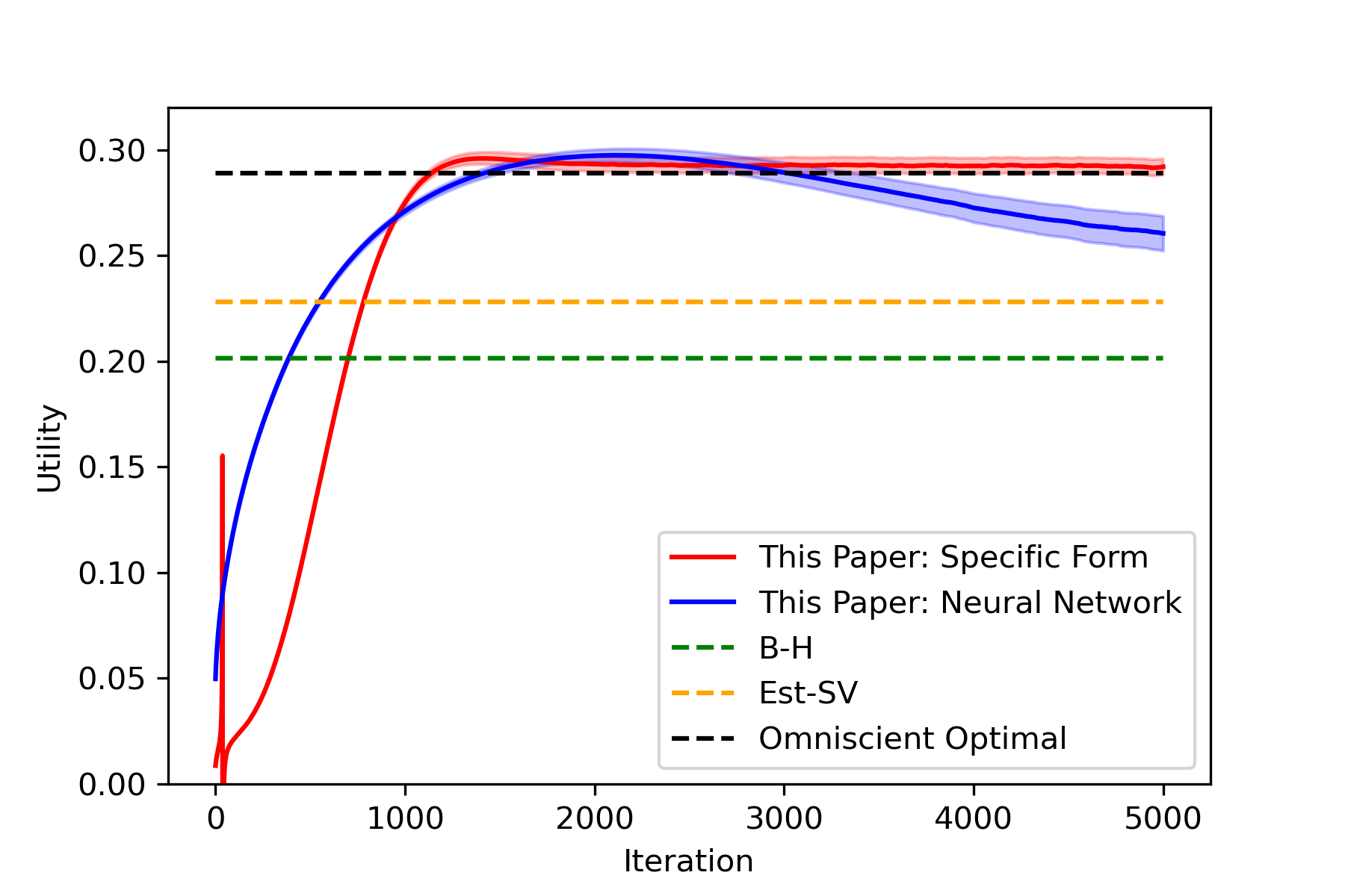
Figure 2: Average utility of various methods on test set as functions of number of training episodes with noisy observation of volatility. Learning curves of various methods when volatility data are contaminated. The width of the shaded area is twice the standard deviation.

6.2 Empirical Study with Real Market Data

We study dynamic allocation between the S&P 500 index and a money market account with $r=2\%$ risk-free interest rate to illustrate the performance of our RL algorithms in the real market. S&P 500 is one of the most actively traded indices and its option market is also highly liquid. Therefore, we can easily obtain volatility-related data from the market. In particular, VIX is an index administered by CBOE (Chicago Board Options Exchange) since 1990 based on option prices that reflects the market-priced average forward-looking volatility of the S&P 500 index, and is widely considered to be a proxy of the instantaneous volatility. VIX itself is a traded future with options written on it. In our empirical study, we take the S&P 500 index as the risky asset and VIX as a proxy for its volatility, both observable. We take data from 1990-01-01 to 2023-06-30 and use the first 10 years (up to 1999-12-31) as the pre-training period and leave the rest as the testing period. During the former period, we apply our offline algorithm, Algorithm 2, to learn the parameters $(\psi,\theta)$ and set the learned ones as the initial parameters for the latter period. Then we use the online algorithm, Algorithm 1, to learn and implement optimal Merton’s strategies as we go. We fix our initial wealth on 2000-01-01 to be 1 dollar and take the risk aversion parameter as $\gamma=3$. The benchmark policies to compare against are still the buy-and-hold (B-H) and the estimate-and-plug-in (Est-SV). We do not allow leverage or borrowing for all the policies under comparison; so if a method suggests taking leverage or short selling, then we truncate the portfolio value to be in the interval $[0,1]$.

Also, to avoid seasonality that depends on the investment horizon, we consider only time-invariant policies, which can be viewed as the limit when the time-to-maturity approaches infinity. This seems reasonable given that we have a rather long testing period. Note that for a stochastic volatility model, such time-invariant policies still result in time-variant portfolios via the (time-variant) instantaneous volatility. The form of the optimal policy in (26) then becomes

$$\operatorname{Mean}(\boldsymbol{\pi}^{*}(g))=C_{1}g^{C_{2}},\;\;\;\operatorname{Var}(\boldsymbol{\pi}^{*}(g))=\frac{\lambda}{\gamma g}$$

for some constants $C_{1},C_{2}$.

The Est-SV is implemented as follows. First, we also restrict to time-invariant policies. We use a rolling window with a length of 10 years to estimate the model parameters and then plug-in to the analytical form of the optimal solution under the SV model. To save computational cost and avoid re-estimating the whole model every day, we only update the estimation of model parameters by maximizing the log-likelihood function along the gradient ascend direction for one time step during the testing period.

A comparison of different methods is summarized in Table 3, in terms of several commonly used metrics including (annualized) return, volatility, Sharpe ratio, (downside) semi-volatility, Sortino ratio, Calmar ratio, maximum drawdown, and recovery time. We see that although RL with neural networks has a slightly lower annualized return than B-H, it achieves the highest risk-adjusted return (the Sharpe ratio), followed by B-H and RL with specific form. Notably, both RL methods have significantly smaller maximum drawdowns and even more significantly quicker recovery times compared with B-H, the market index. This shows that the RL strategies are remarkably more stable and robust.

Table 3: Comparison of out-of-sample performances of different methods from January 2000 to June 2023. We report the (annualized) return (Rtn), volatility (Vol), Sharpe ratio, (downside) semi-volatility (Semi-Vol), Sortino ratio, Calmar ratio, maximum drawdown (MDD), and recovery time (RT). The risk-free interest $r=0.02$.

	Rtn	Vol	Sharpe	Semi-Vol	Sortino	Calmar	MDD	RT
This Paper: Specific Form	0.028	0.072	0.107	0.056	0.139	0.031	0.252	282
This Paper: Neural Network	0.040	0.117	0.172	0.088	0.229	0.059	0.339	211
B-H	0.047	0.198	0.137	0.145	0.188	0.048	0.568	1376
Est-SV	0.016	0.098	-0.043	0.073	-0.058	-0.010	0.441	4249

Table 3 only gives a glance of overall and average performance comparison over 24 years. We can look under the hood by inspecting the wealth trajectories under different policies, presented in Figure 3. It is clear that RL with neural networks outperforms (in terms of portfolio worth) all the others prior to around 2020, taken over by B-H only after 2020. However, both RL portfolios are much more stable than B-H, corroborating the findings of Table 3. In particular, the RL strategies considerably and consistently beat the other two during the first 10 years, 2000–2010. Recall that this is an extremely volatile period, including two bear markets, the dot com bubble burst in the early 2000s and the financial crisis during 2007–2008.

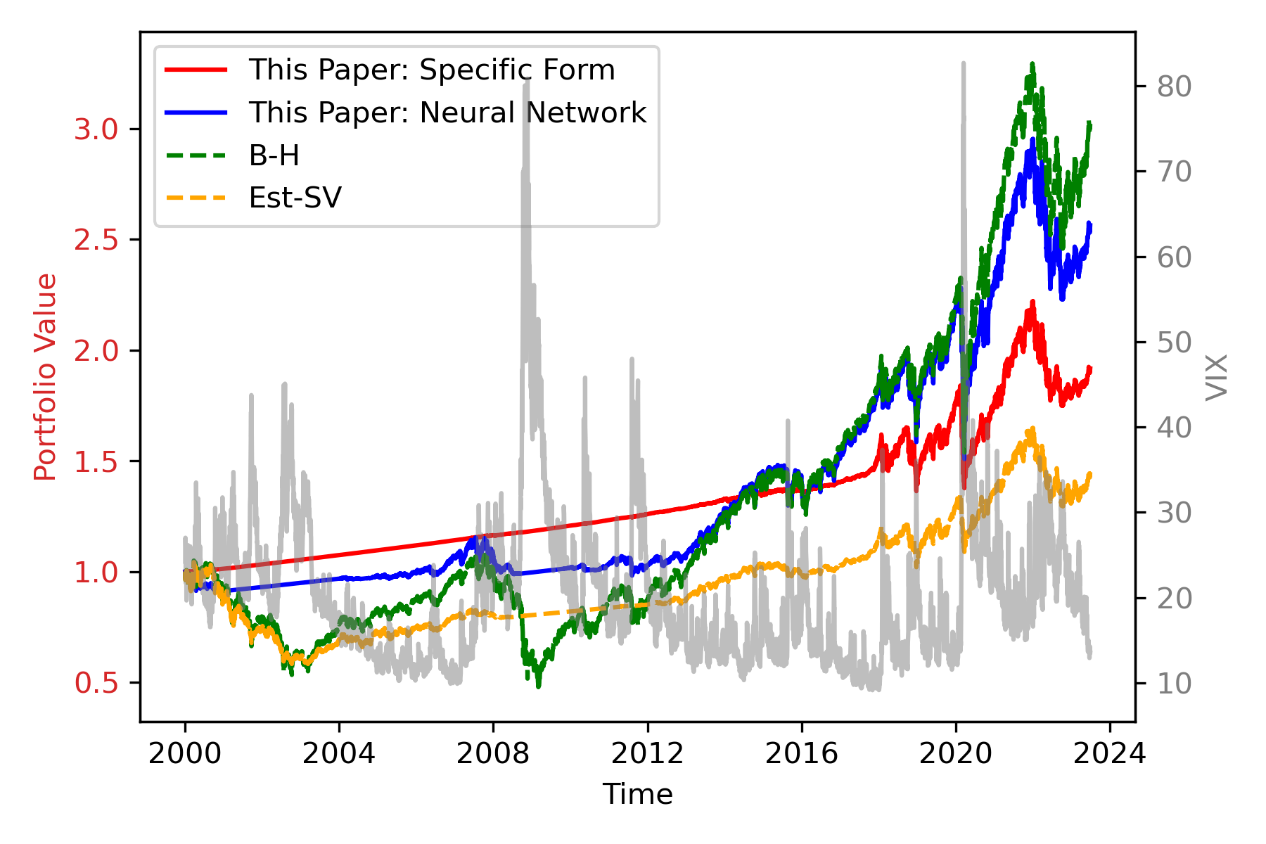
Figure 3: Wealth trajectories of portfolios under different policies. The gray curve is the VIX index whose vertical axis is on the right. The other curves are the trajectories of the portfolio values under different methods and are all normalized to 1 initially.

We further examine the proportions of wealth invested in the risky asset under different strategies, depicted in Figure 4. An interesting observation is that in the first half of the 2000–2010 overall bear period, the two RL-portfolios, especially the one with specific form, do not hold much risky asset as opposed to Est-SV. It demonstrates how the RL approach fundamentally differs from the traditional plug-in approach: Est-SV estimates model parameters statistically based on the market data in the previous 10 years (1990–1999) that had a positive risk premium and that were characteristically different from those in the early 2000s. By contrast, RL learns portfolio strategies through real-time interactions with the market and pivots timely to more conservative ones after the market pivots. On the other hand, all the methods detect buying signals after 2010, while RL with neural networks is the first to react and start to gradually overweigh the risky asset.

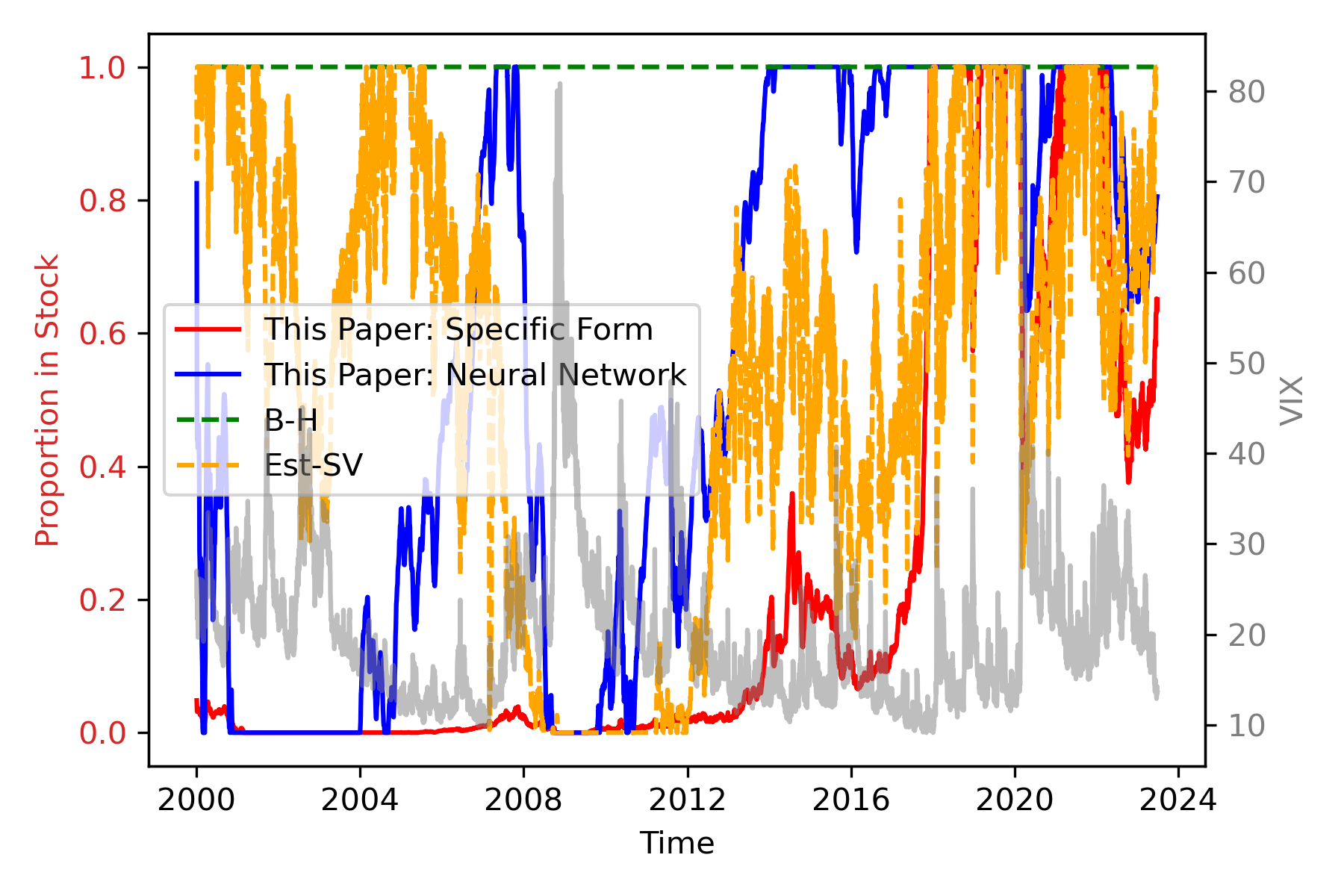
Figure 4: Trajectories of risky proportions under different policies. In our study, proportions invested in S&P 500 are restricted to be between 0 and 1. The gray curve is the VIX index whose vertical axis is on the right. The other curves are the trajectories of the proportions of the risky investment under different methods. The initial allocations of all the methods (except B-H) are based on the pre-training period from 1990 to 1999.

The empirical results indicate, rather decisively, that the RL methods are superior to the conventional Est-SV method in almost all fronts. As for the competition between the two RL algorithms, the one with neural networks outperforms the other by a good margin, contrary to the results from the simulation study. We argue that the reason is because the specific parametric form we adopt follows from a specific 3/2 model, which is almost certainly not valid in the real market, while the flexible structure of neural networks helps to identify other possible forms of investment strategies by exploiting as much as possible the VIX signals.

7 Conclusions

In this paper we study Merton’s asset allocation problem within the continuous-time RL exploratory framework developed by Wang et al. (2020). Inspired by the recursive utility related to habit formation in the decision science and economics literature, we propose a recursive weighting scheme for the entropy regularizer to generate an inherent, path-dependent balance between exploration and exploitation. Such a formulation meanwhile unlocks the optimality of Gaussian exploration in a general incomplete market setting for the CRRA utility. The Gaussian samplers, however, are generally biased, and we present an asymptotic analysis on the bias in terms of the primary temperature parameter.

We then focus on a stochastic volatility environment to devise actor–critic algorithms for learning optimal policies and value functions iteratively. Through policy evaluation and policy update, we show such an iterative procedure yields monotonically improving policies. Finally, we carry out numerical experiments, with both simulated and real market data, to demonstrate the efficiency and robustness of our methods against traditional model-based, plug-in methods.

Gaussian exploration has been widely adopted in RL practice for its intuitive appeal and sampling simplicity. Its optimality has been rigorously established in continuous time only for the LQ setting. This paper seems to be the first to prove the optimality in a non-LQ setting. Equally important, we argue through this paper that biased exploration is rather the rule than an exception, due to the intertwined different random sources, both exogenous and endogenous, in the black-box environment. In the setting of this paper, these random sources include the one driving the stock price, the one driving the factors (which calls for hedging) and the additional randomization injected due to exploration. It remains a fascinating research problem to fully understand the general interactions among these randomness and their impact on learning performance.

8 Motivation of Formulation (5)

We explain the exploratory formulation (5) in a discrete-time setting for easy understanding. First of all, applying Itô’s formula to (3) we obtain that $R_{t}=\log W_{t}^{a}$ follows

$$\mathrm{d}R_{t}=[r+(\mu_{t}-r)a_{t}-\frac{1}{2}\sigma_{t}^{2}a_{t}^{2}]\mathrm{d}t+\sigma_{t}a_{t}\mathrm{d}B_{t},\ \ R_{0}=\log w_{0},$$

where $\mu_{t}\equiv\mu(t,X_{t}),\;\sigma_{t}\equiv\sigma(t,X_{t})$. Divide $[0,T]$ into small intervals of size $\Delta t$. With a portfolio $a_{t}$ applied on the interval $[t,t+\Delta t]$, the incremental change of the log wealth process over $[t,t+\Delta t]$ is

$$\Delta R_{t}=\left[r+(\mu_{t}-r)a_{t}-\frac{1}{2}\sigma_{t}^{2}a_{t}^{2}\right]\Delta t+\sigma_{t}a_{t}\Delta B_{t}.$$

Now, we assume instead that the agent chooses portfolios randomly according to a stochastic policy $\boldsymbol{\pi}$ that is independent of the underlying Brownian motions in the market. In view of the central limit theorem, the limiting distribution is determined only by the first and second moments. Hence we focus on the first and second moments of the randomized policy, and replace $a_{t}$ with $e_{t}+v_{t}\varepsilon_{t}$, where $\varepsilon_{t}$ is a random variable with zero mean and unit variance independent of $B_{t}$ and $\tilde{B}_{t}$ and

$$e_{t}\equiv\operatorname{Mean}(\boldsymbol{\pi}_{t})=\int_{\mathbb{R}}u\boldsymbol{\pi}_{t}(u)\mathrm{d}u,\ \ \mbox{and }\ \ v_{t}\equiv\sqrt{\operatorname{Var}(\boldsymbol{\pi}_{t})}=\sqrt{\int_{\mathbb{R}}u^{2}\boldsymbol{\pi}_{t}(u)\mathrm{d}u-\left(\int_{\mathbb{R}}u\boldsymbol{\pi}_{t}(u)\mathrm{d}u\right)^{2}}.$$

It follows

$$\Delta R_{t} = \left[r+(\mu_{t}-r)(e_{t}+v_{t}\varepsilon_{t})-\frac{1}{2}\sigma_{t}^{2}(e_{t}+v_{t}\varepsilon_{t})^{2}\right]\Delta t+\sigma_{t}(e_{t}+v_{t}\varepsilon_{t})\Delta B_{t}$$

$$= \left[r+(\mu_{t}-r)e_{t}-\frac{1}{2}\sigma_{t}^{2}(e^{2}_{t}+v_{t}^{2})\right]\Delta t+\sigma_{t}e_{t}\Delta B_{t}+\sigma_{t}v_{t}\varepsilon_{t}\Delta B_{t}+Residual_{t},$$

where the residual term, $Residual_{t}$, is given as follows:

$$Residual_{t}=(\mu_{t}-r)v_{t}\varepsilon_{t}\Delta t-\sigma_{t}^{2}e_{t}v_{t}\varepsilon_{t}\Delta t-\sigma_{t}^{2}v^{2}_{t}(\varepsilon^{2}_{t}-1)\Delta t.$$

Since the residual term is a mean zero random variable of size $O(\Delta t)$ and the policy noises $\varepsilon_{t}$ are mutually independent between time intervals, by the law of large numbers, the residual term will vanish when we take the sum over the whole time interval and send $\Delta t$ to zero. Moreover, as $\varepsilon_{t}\Delta B_{t}$ is a mean zero random variable of size $O(\sqrt{\Delta t})$, its summation is asymptotically Gaussian by the central limit theorem. Furthermore, we have $\text{Cov}(\varepsilon_{t}\Delta B_{t},\Delta B_{t})=0$ and $\text{Cov}(\varepsilon_{t}\Delta B_{t},\Delta\tilde{B}_{t})=0$ as $\varepsilon_{t}$ is independent of $B_{t}$ and $\tilde{B}_{t}$. Thus, $\varepsilon_{t}\Delta B_{t}$ can be approximately treated as the increment of another Brownian motion independent of $B_{t}$ and $\tilde{B}_{t}$. It is not hard to verify that

$$\mathbb{E}\left[\Delta R_{t}\right] = \left[r+(\mu_{t}-r)e_{t}-\frac{1}{2}\sigma_{t}^{2}(e^{2}_{t}+v_{t}^{2})\right]\Delta t$$

$$= \left[r+(\mu_{t}-r)\int_{\mathbb{R}}u\boldsymbol{\pi}_{t}(u)\mathrm{d}u-\frac{1}{2}\sigma_{t}^{2}\int_{\mathbb{R}}u^{2}\boldsymbol{\pi}_{t}(u)\mathrm{d}u\right]\Delta t,$$

$$\operatorname{Var}\left[\Delta R_{t}\right] = \sigma_{t}^{2}(e_{t}^{2}+v_{t}^{2})\Delta t+o(\Delta t)=\sigma_{t}^{2}\int_{\mathbb{R}}u^{2}\boldsymbol{\pi}_{t}(u)\mathrm{d}u\Delta t+o(\Delta t),$$

$$\text{Cov}\left[\Delta R_{t},\Delta X_{t}\right] = \rho\nu\sigma_{t}e_{t}\Delta t+o(\Delta t)=\rho\nu\sigma_{t}\int_{\mathbb{R}}u\boldsymbol{\pi}_{t}(u)\mathrm{d}u\Delta t+o(\Delta t).$$

This suggests that at the continuous-time limit, $R$ satisfies the following SDE

$$\mathrm{d}R_{t}= \left[r+(\mu_{t}-r)\operatorname{Mean}(\boldsymbol{\pi}_{t})-\frac{1}{2}\sigma_{t}^{2}(\operatorname{Mean}(\boldsymbol{\pi}_{t}))^{2}-\frac{1}{2}\sigma_{t}^{2}\operatorname{Var}(\boldsymbol{\pi}_{t})\right]\mathrm{d}t$$

$$\;\;+\sigma_{t}\left[\operatorname{Mean}(\boldsymbol{\pi}_{t})\mathrm{d}B_{t}+\sqrt{\operatorname{Var}(\boldsymbol{\pi}_{t})}\mathrm{d}\bar{B}_{t}\right],\ \ R_{0}=\log w_{0},$$

where $\bar{B}_{t}$ is another Brownian motion that is mutually independent of $B_{t}$ and $\tilde{B}_{t}$. As discussed earlier, $\bar{B}_{t}$ is introduced to model the noise caused by exploration and can be regarded as a “random number generator” to generate a randomized policy. The coefficient of the $\mathrm{d}\bar{B}_{t}$ term involves the variance of $\boldsymbol{\pi}_{t}$, measuring how much additional noise is introduced into the system.

Applying Itô’s formula to the above equation we get that $W^{\boldsymbol{\pi}}_{t}=e^{R_{t}}$ satisfies the exploratory dynamics (5). As indicated by the above analysis, this exploratory formulation captures the information up to the second order.

9 Regularization under Different Temperature Schemes

In this section we discuss two alternative temperature schemes for regularization, and explain the drawbacks of these formulations compared with our recursive formulation.

9.1 Constant Temperature

With the exploratory dynamics given in (5), if we were to use a constant temperature as in Wang et al. (2020) with the objective function

$$\mathbb{E}\left[\int_{t}^{T}\lambda\mathcal{H}(\boldsymbol{\pi}_{s})\mathrm{d}s+U(W_{T}^{\boldsymbol{\boldsymbol{\pi}}})\Big{|}W_{t}^{\boldsymbol{\pi}}=w,X_{t}=x\right],$$

then the associated HJB equation would be

$$\frac{\partial V}{\partial t}+\sup_{\boldsymbol{\pi}}\Bigg{\{}\Big{(}r+\big{(}\mu(t,x)-r\big{)}\operatorname{Mean}(\boldsymbol{\pi})\Big{)}wV_{w}+\frac{1}{2}\sigma^{2}(t,x)\Big{(}\operatorname{Mean}(\boldsymbol{\pi})^{2}+\operatorname{Var}(\boldsymbol{\pi})\Big{)}w^{2}V_{ww}$$ (32)

$$+m(t,x)V_{x}+\frac{1}{2}\nu^{2}(t,x)V_{xx}+\rho\nu(t,x)\sigma(t,x)\operatorname{Mean}(\boldsymbol{\pi})wV_{wx}+\lambda\mathcal{H}(\boldsymbol{\pi})\Bigg{\}}=0,$$

with the terminal condition $V(T,w,x)=U(w)=\frac{w^{1-\gamma}-1}{1-\gamma}$.

Similar to Wang et al. (2020), we can solve the maximization problem on the left-hand side of (32) and apply the verification theorem to conclude that the optimal policy is a normal distribution with mean

$$\frac{\big{(}\mu(t,x)-r\big{)}V_{w}}{-\sigma^{2}(t,x)wV_{ww}}+\frac{\rho\nu(t,x)V_{wx}}{-\sigma(t,x)wV_{ww}},$$

and variance

$$\frac{\lambda}{-\sigma^{2}(t,x)w^{2}V_{ww}}.$$

Plugging the above into (32), the equation becomes

$$\frac{\partial V}{\partial t}+rwV_{w}+m(t,x)V_{x}+\frac{1}{2}\nu^{2}(t,x)V_{xx}+\frac{\lambda}{2}\log 2\pi$$ (33)

$$-\frac{\bigg{(}\big{(}\mu(t,x)-r\big{)}V_{w}+\rho\nu(t,x)\sigma(t,x)V_{wx}\bigg{)}^{2}}{2\sigma^{2}(t,x)V_{ww}}+\frac{\lambda}{2}\log\frac{\lambda}{-\sigma^{2}(t,x)w^{2}V_{ww}}=0.$$

This PDE generally admits neither a separable nor a closed-form solution due to a lack of the homothetic property. As a result, analytical forms of the optimal value function and optimal policy are both unavailable, making it hard to parameterize these functions in simpler forms and carry out a theoretical analysis.

9.2 Wealth-Dependent Temperature

In order to obtain a simpler HJB equation, we could consider a wealth-dependent temperature parameter. For example, for CRRA utility, we could take $\lambda(t,w,x)=\lambda w^{1-\gamma}$ where $\gamma\neq 1$. The derivations of (32) and (33) are similar by replacing $\lambda$ with $\lambda w^{1-\gamma}$. With this wealth-dependent weighting scheme for exploration, the problem becomes homothetic in wealth with degree $1-\gamma$; hence the value function admits the form $V(t,w,x)=\frac{w^{1-\gamma}v(t,x)}{1-\gamma}+g(t)$, where $g$ and $v$ satisfy

$$(1-\gamma)g^{\prime}-(1-\gamma)g=\frac{\partial v}{\partial t}+mv_{x}+\frac{\nu^{2}}{2}v_{xx},\ g(T,x)=-\frac{1}{1-\gamma},$$

$$\frac{\partial v}{\partial t}+(1-\gamma)rv+mv_{x}+\frac{\nu^{2}}{2}v_{xx}+\lambda\frac{1-\gamma}{2}\log\frac{2\pi}{\gamma\sigma^{2}v}+\frac{(1-\gamma)\big{(}(\mu-r)v+\rho\nu\sigma v_{x}\big{)}^{2}}{2\gamma\sigma^{2}v},\ v(T,x)=1.$$

Consequently, the optimal policy is a normal distribution with mean $\frac{\mu(t,x)-r}{\gamma\sigma^{2}(t,x)}+\frac{\rho\nu(t,x)v_{x}(t,x)}{\gamma\sigma(t,x)v(t,x)}$ and variance $\frac{\lambda}{\gamma\sigma^{2}(t,x)v(t,x)}$.

The major difference between this formulation and the recursive one is that there is an extra term $v(t,x)$ in the denominator of the optimal exploration variance of the former, which may result in an arbitrarily large exploratory variance within a finite time period and consequently the non-existence of an optimal policy. For example, in the Black–Scholes case ($m,\nu\equiv 0$), $v$ is independent of $x$ and satisfies an ODE whose solution will reach $0$ with some choice of the coefficients. Specifically, $v(t)=\varphi(T-t)$, where $\varphi$ satisfies an ODE:

$$\varphi^{\prime}(\tau)=(1-\gamma)\Big{(}(r+\frac{(\mu-r)^{2}}{2\gamma\sigma^{2}})\varphi(\tau)+\frac{\lambda}{2}\log\frac{2\pi\lambda}{\gamma\sigma^{2}}-\frac{\lambda}{2}\log\varphi(\tau)\Big{)},\ \varphi(0)=1.$$ (34)

We have the following theorem.

Theorem 9.1

If $\gamma>1$ and $r+\frac{(\mu-r)^{2}}{2\gamma\sigma^{2}}+\frac{\lambda}{2}\log\frac{2\pi\lambda}{\gamma\sigma^{2}}<0$, then the solution to (34) reaches $0$ in a finite time.

10 Recursive Regularizer for CARA Utility

The recursive utility also works for the CARA utility, for which we use the dollar amount invested in the risky asset as the control (portfolio) variable, and denote by $\boldsymbol{\pi}$ the corresponding probability-density-valued control. The wealth process under $\boldsymbol{\pi}$ is

$$\mathrm{d}W^{\boldsymbol{\pi}}_{t}=\left[rW^{\boldsymbol{\pi}}_{t}+(\mu(t,X_{t})-r)\operatorname{Mean}(\boldsymbol{\pi}_{t})\right]\mathrm{d}t+\sigma(t,X_{t})\left[\operatorname{Mean}(\boldsymbol{\pi}_{t})\mathrm{d}B_{t}+\sqrt{\operatorname{Var}(\boldsymbol{\pi}_{t})}\mathrm{d}\bar{B}_{t}\right].$$ (35)

Consider the following regularized objective function:

$$J^{\boldsymbol{\pi}}_{t}:=\mathbb{E}\left[\int_{t}^{T}-\lambda J_{s}^{\boldsymbol{\pi}}\mathcal{H}(\boldsymbol{\pi}_{s})\mathrm{d}s+U(W_{T}^{\boldsymbol{\pi}})\Big{|}\mathcal{F}_{t}\right],$$ (36)

where $U(x)=-\frac{1}{\gamma}e^{-\gamma x}$. Under this recursive weighting scheme, the optimal policy is given by

$$\boldsymbol{\pi}^{*}(t,x)=\mathcal{N}\bigg{(}\big{(}\frac{\mu(t,x)-r}{\gamma\sigma^{2}(t,x)}-\frac{\rho\nu(t,x)}{\sigma(t,x)}u_{x}(t,x)\big{)}e^{-r(T-t)},\frac{\lambda}{\gamma^{2}\sigma^{2}(t,x)}e^{-2r(T-t)}\bigg{)},$$

where $u$ satisfies

$$u_{t}+m(t,x)u_{x}+\frac{1}{2}\nu^{2}(t,x)(-\gamma u_{x}^{2}+u_{xx})+\frac{\gamma\sigma^{2}(t,x)}{2}\left(\frac{\mu(t,x)-r}{\gamma\sigma^{2}(t,x)}-\frac{\rho\nu(t,x)}{\sigma(t,x)}u_{x}\right)^{2}$$

$$+\frac{\lambda}{2\gamma}\log\frac{2\pi\lambda}{\gamma^{2}\sigma^{2}(t,x)e^{2r(T-t)}}=0,\ \ \ u(T,x)=0,$$

and the associated optimal value function is $V(t,w,x)=-\frac{1}{\gamma}\exp(-\gamma u(t,x)-\gamma e^{r(T-t)}w)$. Hence we can develop RL theory and algorithms parallel to the CRRA utility. Details are left to the interested readers.

11 A BSDE Perspective

The optimal portfolio processes with parameter $\lambda$ in the exploratory problem can also be characterized by a BSDE.

Theorem 11.1

Suppose the following quadratic BSDE admits a unique solution

$$\left\{\begin{aligned} \mathrm{d}Y_{t}^{*(\lambda)}=&-\Bigg{\{}(1-\gamma)\Big{[}\frac{\lambda}{2}\log\frac{2\pi\lambda}{\gamma\sigma_{t}^{2}}+r+\frac{(\mu_{t}-r+\rho\sigma_{t}Z^{*(\lambda)}_{t})^{2}}{2\gamma\sigma_{t}^{2}}\Big{]}+\frac{1}{2}{Z_{t}^{*(\lambda)}}^{2}\Bigg{\}}\mathrm{d}t+Z_{t}^{*(\lambda)}\mathrm{d}B_{t}^{X},\\ Y^{*(\lambda)}_{T}=&0.\end{aligned}\right.$$ (37)

Then the optimal exploratory control is given by

$$\boldsymbol{\pi}^{*(\lambda)}_{t}=\mathcal{N}\Big{(}\frac{\mu_{t}-r+\rho\sigma_{t}Z^{*(\lambda)}_{t}}{\gamma\sigma^{2}_{t}},\frac{\lambda}{\gamma\sigma_{t}^{2}}\Big{)}.$$

The solution to BSDE (37) corresponds to the PDE (15) in Theorem 3.1. The process $Y^{*(\lambda)}$ can be interpreted as an auxiliary process in the martingale duality theory, which stipulates that

$$\left(V^{\boldsymbol{\pi}}_{t}+\int_{0}^{t}\lambda\mathcal{H}(\boldsymbol{\pi}_{s})\big{[}(1-\gamma)V^{\boldsymbol{\pi}}_{s}+1\big{]}\mathrm{d}s\right)e^{Y_{t}^{*(\lambda)}}$$

is a supermartingale for any portfolio control $\boldsymbol{\pi}_{t}$ and a martingale when $\boldsymbol{\pi}_{t}=\boldsymbol{\pi}^{*(\lambda)}_{t}$, where $V^{\boldsymbol{\pi}}_{t}=\frac{{w_{t}^{\boldsymbol{\pi}}}^{1-\gamma}}{1-\gamma}e^{Y_{t}^{*(\lambda)}}-\frac{1}{1-\gamma}$ is the value function evaluated along the optimal wealth trajectories. Moreover, when $\lambda=0$, the above result reduces to the classical one which was first derived by Hu et al. (2005).

The BSDE (37) offers important insights about the connection between the classical problem ($\lambda=0$) and the exploratory one ($\lambda>0$), some of them consistent with the unbiasedness discussion in Subsection 3.2. First, the only difference between the classical and exploratory problems is the extra term, $\frac{(1-\gamma)\lambda}{2}\log\frac{2\pi\lambda}{\gamma\sigma_{t}^{2}}$, in the driver of (37). This term becomes a deterministic function of $t$ when $\gamma=1$ (log-utility) or when $\sigma_{t}$ is deterministic, in which case $Z^{*(\lambda)}=Z^{*(0)}$. Hence the optimal solution of the exploratory problem has a mean that coincides with the classical solution, or the former is unbiased. Incidentally, this is consistent with an earlier result of Dai et al. (2023) in the mean–variance analysis for the log utility. Second, when $\rho=0$, i.e., the market factors evolve independently from the stock price, the optimal exploratory policy is also unbiased, even if $Z^{*(\lambda)}\neq Z^{*(0)}$ in general. This is intuitive because hedging is not necessary in this case. A special case is when the market factor $X$ is deterministic, in which case the source of randomness $B^{X}_{t}$ vanishes leading to $Z^{*(\lambda)}=Z^{*(0)}=0$ and hence the optimal exploration is unbiased. Otherwise, optimal exploratory policies are in general biased in stochastic volatility models when $\sigma_{t}$ is a function of the stochastic factor process $X_{t}$ and the power of the utility $\gamma\neq 1$.

12 Additional Numerical Results

In the main paper, we generate a training dataset that has a length of 20 years, and each time we sample a subsequence with a length of 1 year as one episode for training. This is to capture the practical situation in which financial data are always limited. However, in a simulation study we can generate as large an amount of data as we desire. Here we report the results of such a “thought experiment” when data are unlimited. Specifically, in each episode, we generate independent one-year data from the given dynamics for training. Figure 5 illustrates the learning curves of the two RL methods, where average utilities are computed on an independent, fixed test set with 10000 wealth trajectories. Both curves, based on specific forms and neural networks, converge to the omniscient optimal utility after about 3000 independent episodes.

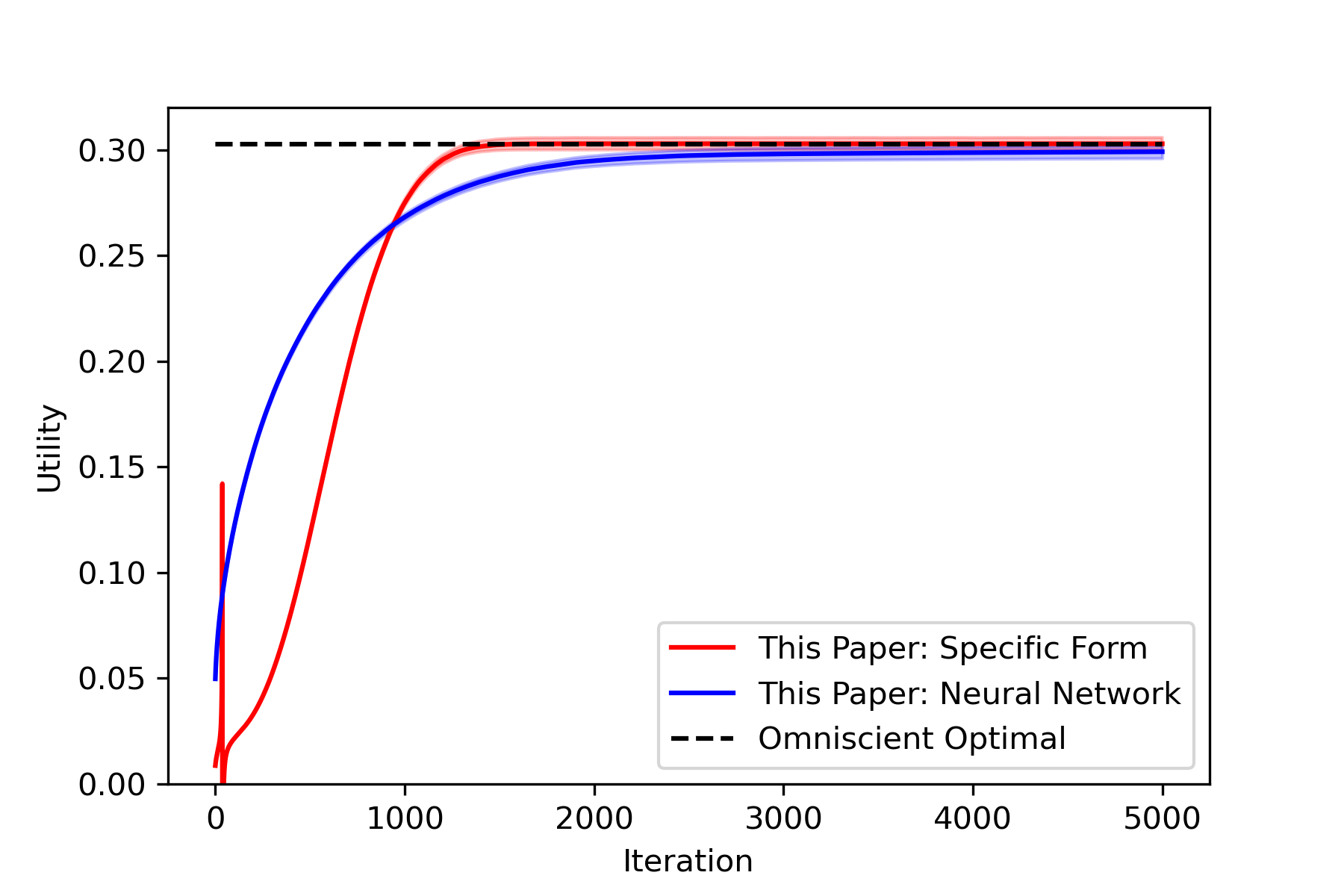
Figure 5: Average utility of RL algorithms on the test set as functions of the number of training episodes. In each episode, independent one-year data are generated from the model dynamics for training. The width of the shaded area is twice the standard deviation.

13 Proof of Statements

13.1 Proof of Proposition 2.2

Recall that the recursive utility satisfies the BSDE (8). Given an admissible control $\boldsymbol{\pi}$, the condition $(ii)$ in Definition 2.1 guarantees that the solution to (5) exists, and can be written as

$$W_{t}^{\boldsymbol{\pi}}=w_{0}\exp\bigg{\{}\int_{0}^{t} \left[r+(\mu_{s}-r)\operatorname{Mean}(\boldsymbol{\pi}_{s})+\frac{1}{2}\sigma_{s}^{2}\left(\operatorname{Mean}(\boldsymbol{\pi}_{s})^{2}+\operatorname{Var}(\boldsymbol{\pi}_{s})\right)\right]\mathrm{d}s$$

$$+\sigma_{s}\left[\operatorname{Mean}(\boldsymbol{\pi}_{s})\mathrm{d}B_{s}+\sqrt{\operatorname{Var}(\boldsymbol{\pi}_{s})}\mathrm{d}\bar{B}_{s}\right]\bigg{\}}>0.$$

In addition, (8) is a linear BSDE, and the condition $(iii)$ in Definition 2.1 ensures that $U(W_{T}^{\boldsymbol{\pi}})$ and $\{\lambda(t,X_{t})\mathcal{H}(\boldsymbol{\pi}_{t})\}_{t\in[0,T]}$ are respectively square integrable variable and process. Hence by El Karoui et al. (1997, Proposition 2.2), (8) admits a unique, square-integrable solution.

Define $\tilde{Y}^{\boldsymbol{\pi}}_{t}:=(1-\gamma)J_{t}^{\boldsymbol{\pi}}+1$. Applying Itô’s lemma, we obtain that $\tilde{Y}^{\boldsymbol{\pi}}$ solves the following BSDE:

$$\mathrm{d}\tilde{Y}^{\boldsymbol{\pi}}_{t}=-(1-\gamma)\lambda(t,X_{t})\mathcal{H}(\boldsymbol{\pi}_{t})\tilde{Y}^{\boldsymbol{\pi}}_{t}\mathrm{d}t+(1-\gamma)\tilde{\mathbf{Z}}^{\boldsymbol{\pi}}_{t}\cdot\mathrm{d}\mathbf{B}_{t},\ \tilde{Y}^{\boldsymbol{\pi}}_{T}=({W_{T}^{\boldsymbol{\pi}}})^{1-\gamma}>0.$$

From the comparison principle of linear BSDEs (see El Karoui et al. 1997, Corollary 2.2), it follows that $\tilde{Y}^{\boldsymbol{\pi}}_{t}>0$ almost surely.

13.2 Proof of Theorem 3.1

First, let us show how to deduce (16) from (14). Note that the “supermum” in (14) can be achieved via a two-stage optimization procedure: first maximize over distributions with a fixed mean and variance pair, and then maximize over all possible such pairs. For the first problem, the entropy is maximized at a normal distribution with the fixed mean and variance, with the maximum entropy value $\mathcal{H}(\boldsymbol{\pi})=\frac{1}{2}\log\big{(}2\pi e\operatorname{Var}(\boldsymbol{\pi})\big{)}$ where $\operatorname{Var}(\boldsymbol{\pi})$ is the given fixed variance. Therefore, (14) can be simplified as

$$\frac{\partial V}{\partial t}+\sup_{\operatorname{Mean}(\boldsymbol{\pi}),\operatorname{Var}(\boldsymbol{\pi})}\Bigg{\{}\Big{(}r+\big{(}\mu(t,x)-r\big{)}\operatorname{Mean}(\boldsymbol{\pi})\Big{)}wV_{w}+\frac{1}{2}\sigma^{2}(t,x)\Big{(}\operatorname{Mean}(\boldsymbol{\pi})^{2}+\operatorname{Var}(\boldsymbol{\pi})\Big{)}w^{2}V_{ww}$$ (38)

$$+m(t,x)V_{x}+\frac{1}{2}\nu^{2}(t,x)V_{xx}+\rho\nu(t,x)\sigma(t,x)\operatorname{Mean}(\boldsymbol{\pi})wV_{wx}+\frac{\lambda(t,x)}{2}\log\big{(}2\pi e\operatorname{Var}(\boldsymbol{\pi})\big{)}\big{[}(1-\gamma)V+1\big{]}\Bigg{\}}$$

$$=0.$$

To analyze the above PDE, we start with the ansatz that $V(t,w,x)=\frac{w^{1-\gamma}}{1-\gamma}v(t,x)-\frac{1}{1-\gamma}$ for some function $v$. Then (38) becomes

$$\frac{w^{1-\gamma}}{1-\gamma}\frac{\partial v}{\partial t}+\sup_{\operatorname{Mean}(\boldsymbol{\pi}),\operatorname{Var}(\boldsymbol{\pi})}\Bigg{\{}\Big{(}r+\big{(}\mu(t,x)-r\big{)}\operatorname{Mean}(\boldsymbol{\pi})\Big{)}w^{1-\gamma}v-\frac{\gamma}{2}\sigma^{2}(t,x)\Big{(}\operatorname{Mean}(\boldsymbol{\pi})^{2}+\operatorname{Var}(\boldsymbol{\pi})\Big{)}w^{1-\gamma}v$$ (39)

$$+m(t,x)\frac{w^{1-\gamma}}{1-\gamma}v_{x}+\frac{1}{2}\nu^{2}(t,x)\frac{w^{1-\gamma}}{1-\gamma}v_{xx}+\rho\nu(t,x)\sigma(t,x)\operatorname{Mean}(\boldsymbol{\pi})w^{1-\gamma}v_{x}+\frac{\lambda(t,x)}{2}\log\big{(}2\pi e\operatorname{Var}(\boldsymbol{\pi})\big{)}w^{1-\gamma}v\Bigg{\}}=0.$$

If $v>0$ (to be verified later), then the first-order conditions of the maximization problem on the left-hand side of the above equation yield the maximizers

$$\operatorname{Mean}(\boldsymbol{\pi}^{*})=\frac{\mu(t,x)-r}{\gamma\sigma^{2}(t,x)}+\frac{\rho\nu(t,x)v_{x}(t,x)}{\gamma\sigma(t,x)v(t,x)},\;\;\;\operatorname{Var}(\boldsymbol{\pi}^{*})=\frac{\lambda(t,x)}{\gamma\sigma^{2}(t,x)}.$$ (40)

Plugging the above into (39) and canceling the term $w^{1-\gamma}$, we have that $v$ satisfies the following nonlinear PDE:

$$\frac{\partial v}{\partial t} +(1-\gamma)rv+m(t,x)v_{x}+\frac{1}{2}\nu^{2}(t,x)v_{xx}+\frac{(1-\gamma)\lambda(t,x)v}{2}\log\frac{2\pi\lambda(t,x)}{\gamma\sigma^{2}(t,x)}$$ (41)

$$+\frac{1-\gamma}{2\gamma}\Big{[}\frac{\big{(}\mu(t,x)-r\big{)}^{2}}{\sigma^{2}(t,x)}v+\frac{2\rho\big{(}\mu(t,x)-r\big{)}\nu(t,x)}{\sigma(t,x)}v_{x}+\rho^{2}\nu^{2}(t,x)\frac{v_{x}^{2}}{v}\Big{]}=0,$$

with the terminal condition $v(T,x)=1$.

Letting $u$ be the solution to (15), we can directly verify that $v(t,x)=e^{u(t,x)}>0$ solves (41). The desired expression (16) now follows from (40).

Next we prove that the policy with (16) is optimal and $V(t,w,x)=\frac{w^{1-\gamma}e^{u(t,x)}-1}{1-\gamma}$ is the optimal value function. Denote $K_{t}^{\boldsymbol{\pi}}=\int_{0}^{t}\lambda(s,X_{s})(1-\gamma)\mathcal{H}(\boldsymbol{\pi}_{s})\mathrm{d}s$. Apply Itô’s formula to $e^{K_{t}}V(t,W^{\boldsymbol{\pi}}_{t},X_{t})$ to get

$$\begin{split}&\mathrm{d}\left(e^{K_{t}^{\boldsymbol{\pi}}}V(t,W^{\boldsymbol{\pi}}_{t},X_{t})\right)\\ =&\bigg{\{}\frac{\partial V}{\partial t}+\left[r+(\mu(t,X_{t})-r)\operatorname{Mean}(\boldsymbol{\pi}_{t})\right]W^{\boldsymbol{\pi}}_{t}V_{w}+m(t,X_{t})V_{x}+\frac{1}{2}\sigma^{2}(t,X_{t})\left[\operatorname{Mean}(\boldsymbol{\pi}_{t})^{2}+\operatorname{Var}(\boldsymbol{\pi}_{t})\right](W^{\boldsymbol{\pi}}_{t})^{2}V_{ww}\\ &+\frac{1}{2}\nu^{2}(t,X_{t})V_{xx}+\rho\nu(t,X_{t})\sigma(t,X_{t})\operatorname{Mean}(\boldsymbol{\pi}_{t})W^{\boldsymbol{\pi}}_{t}V_{w}+\lambda(1-\gamma)\mathcal{H}(\boldsymbol{\pi}_{t})V\bigg{\}}e^{K_{t}^{\boldsymbol{\pi}}}\mathrm{d}t\\ &+\bigg{\{}\left[\sigma(t,X_{t})\operatorname{Mean}(\boldsymbol{\pi}_{t})W^{\boldsymbol{\pi}}_{t}V_{w}+\rho\nu(t,X_{t})V_{x}\right]\mathrm{d}B_{t}\\ &+\sqrt{1-\rho^{2}}\nu(t,X_{t})V_{x}\mathrm{d}\tilde{B}_{t}+\sqrt{\operatorname{Var}(\boldsymbol{\pi}_{t})}\sigma(t,X_{t})W^{\boldsymbol{\pi}}_{t}V_{w}\mathrm{d}\bar{B}_{t}\bigg{\}}e^{K_{t}^{\boldsymbol{\pi}}}.\end{split}$$

Define a sequence of stopping times $\tau_{n}=\inf\{t\geq 0:|X_{t}|\vee(W_{t}^{\boldsymbol{\pi}})^{1-\gamma}\vee e^{K_{t}^{\boldsymbol{\pi}}}\geq n\}$. Then by (38), we have

$$e^{K_{T\wedge\tau_{n}}^{\boldsymbol{\pi}}}V(T\wedge\tau_{n},W^{\boldsymbol{\pi}}_{T\wedge\tau_{n}},X_{T\wedge\tau_{n}})-V(0,W^{\boldsymbol{\pi}}_{0},X_{0})$$

$$\leq \int_{0}^{T\wedge\tau_{n}}-\lambda(s,X_{s})\mathcal{H}(\boldsymbol{\pi}_{s})e^{K_{s}^{\boldsymbol{\pi}}}\mathrm{d}s+e^{K_{s}^{\boldsymbol{\pi}}}(W^{\boldsymbol{\pi}}_{s})^{1-\gamma}e^{u(s,X_{s})}\bigg{\{}\left[\sigma(s,X_{s})\operatorname{Mean}(\boldsymbol{\pi}_{s})+\rho\nu(s,X_{s})\frac{u_{x}(s,X_{s})}{1-\gamma}\right]\mathrm{d}B_{s}$$

$$+\sqrt{1-\rho^{2}}\nu(s,X_{s})\frac{u_{x}(s,X_{s})}{1-\gamma}\mathrm{d}\tilde{B}_{s}+\sqrt{\operatorname{Var}(\boldsymbol{\pi}_{s})}\sigma(s,X_{s})\mathrm{d}\bar{B}_{s}\bigg{\}},$$

while “$=$” holds when $\boldsymbol{\pi}=\boldsymbol{\pi}^{*}$ as given in (16).

Recall that $u$ and its derivatives have polynomial growth in $x$; hence we have an estimate about the quadratic variation term above

$$\mathbb{E}\Bigg{[}\int_{0}^{T\wedge\tau_{n}}e^{2K_{s}^{\boldsymbol{\pi}}}(W^{\boldsymbol{\pi}}_{s})^{2(1-\gamma)}e^{2u(s,X_{s})}\bigg{\{}\left[\sigma(s,X_{s})\operatorname{Mean}(\boldsymbol{\pi}_{s})+\rho\nu(s,X_{s})\frac{u_{x}(s,X_{s})}{1-\gamma}\right]^{2}$$

$$+(1-\rho^{2})\nu^{2}(s,X_{s})\frac{u_{x}^{2}(s,X_{s})}{(1-\gamma)^{2}}+\operatorname{Var}(\boldsymbol{\pi}_{s})\sigma^{2}(s,X_{s})\bigg{\}}\mathrm{d}s\Bigg{]}$$

$$\leq \mathbb{E}\left[\int_{0}^{T}C_{n}\bigg{\{}\sigma^{2}(s,X_{s})\left[\operatorname{Mean}(\boldsymbol{\pi}_{s})^{2}+\operatorname{Var}(\boldsymbol{\pi}_{s})\right]+1\bigg{\}}\mathrm{d}s\right]$$

for some constants $C_{n}>0$. Therefore, the expectations of the corresponding stochastic integrals are all 0. When $\boldsymbol{\pi}$ is admissible, by the condition ($ii$) in Definition 2.1, we deduce

$$V(0,w_{0},x_{0})$$

$$\geq \mathbb{E}\left[e^{K_{T\wedge\tau_{n}}^{\boldsymbol{\pi}}}V(T\wedge\tau_{n},W^{\boldsymbol{\pi}}_{T\wedge\tau_{n}},X_{T\wedge\tau_{n}})+\int_{0}^{T\wedge\tau_{n}}\lambda(s,X_{s})\mathcal{H}(\boldsymbol{\pi}_{s})e^{K_{s}^{\boldsymbol{\pi}}}\mathrm{d}s\right]$$

$$= \mathbb{E}\left[e^{K_{T\wedge\tau_{n}}^{\boldsymbol{\pi}}}\frac{(W^{\boldsymbol{\pi}}_{T\wedge\tau_{n}})^{1-\gamma}}{1-\gamma}e^{u(T\wedge\tau_{n},X_{T\wedge\tau_{n}})}-\frac{e^{K_{T\wedge\tau_{n}}^{\boldsymbol{\pi}}}}{1-\gamma}+\int_{0}^{T\wedge\tau_{n}}\lambda(s,X_{s})\mathcal{H}(\boldsymbol{\pi}_{s})e^{K_{s}^{\boldsymbol{\pi}}}\mathrm{d}s\right]$$

$$= \mathbb{E}\left[e^{K_{T}^{\boldsymbol{\pi}}}\frac{(W^{\boldsymbol{\pi}}_{T})^{1-\gamma}}{1-\gamma}\mathbbm{1}_{\{\tau_{n}>T\}}+e^{K_{\tau_{n}}^{\boldsymbol{\pi}}}\frac{(W^{\boldsymbol{\pi}}_{\tau_{n}})^{1-\gamma}}{1-\gamma}e^{u(\tau_{n},X_{\tau_{n}})}\mathbbm{1}_{\{\tau_{n}\leq T\}}-\frac{e^{K_{T\wedge\tau_{n}}^{\boldsymbol{\pi}}}}{1-\gamma}+\int_{0}^{T\wedge\tau_{n}}\lambda(s,X_{s})\mathcal{H}(\boldsymbol{\pi}_{s})e^{K_{s}^{\boldsymbol{\pi}}}\mathrm{d}s\right].$$

By the condition ($iii$) in Definition 2.1, we have

$$\mathbb{E}\left[\int_{0}^{T}\lambda(t,X_{t})|\mathcal{H}(\boldsymbol{\pi}_{t})|e^{K_{t}^{\boldsymbol{\pi}}}\mathrm{d}t\right]\leq\mathbb{E}\left[\int_{0}^{T}\lambda(t,X_{t})|\mathcal{H}(\boldsymbol{\pi}_{t})|e^{\int_{0}^{t}\lambda|1-\gamma||\mathcal{H}(\boldsymbol{\pi}_{s})|\mathrm{d}s}\mathrm{d}t\right]$$

$$\leq \mathbb{E}\left[\int_{0}^{T}\lambda(t,X_{t})|\mathcal{H}(\boldsymbol{\pi}_{t})|\mathrm{d}te^{\int_{0}^{T}\lambda|1-\gamma||\mathcal{H}(\boldsymbol{\pi}_{s})|\mathrm{d}s}\right]$$

$$\leq \left(\mathbb{E}\left[\left(\int_{0}^{T}\lambda(t,X_{t})|\mathcal{H}(\boldsymbol{\pi}_{t})|\mathrm{d}t\right)^{2}\right]\right)^{1/2}\left(\mathbb{E}\left[e^{\int_{0}^{T}2\lambda|1-\gamma||\mathcal{H}(\boldsymbol{\pi}_{s})|\mathrm{d}s}\right]\right)^{1/2}<\infty,$$

and

$$\mathbb{E}\left[e^{K^{\boldsymbol{\pi}}_{T}}(W^{\boldsymbol{\pi}}_{T})^{1-\gamma}\right]\leq\left(\mathbb{E}\left[e^{\int_{0}^{T}2\lambda|1-\gamma||\mathcal{H}(\boldsymbol{\pi}_{s})|\mathrm{d}s}\right]\right)^{1/2}\left(\mathbb{E}\left[(W^{\boldsymbol{\pi}}_{T})^{2-2\gamma}\right]\right)^{1/2}<\infty.$$

Taking $\limsup_{n\to\infty}$, we conclude from the dominated convergence theorem and Fatou’s lemma that

$$V(0,w_{0},x_{0})\geq\mathbb{E}\left[e^{K_{T}^{\boldsymbol{\pi}}}U(W_{T}^{\boldsymbol{\pi}})+\int_{0}^{T}\lambda(s,X_{s})\mathcal{H}(\boldsymbol{\pi}_{s})e^{K_{s}^{\boldsymbol{\pi}}}\mathrm{d}s\right]=J_{0}^{\boldsymbol{\pi}}.$$

To show “$=$” for $\boldsymbol{\pi}^{*}$, we can directly verify that $V_{t}=V(t,W_{t}^{\boldsymbol{\pi}^{*}},X_{t})$ satisfies the BSDE (8), and hence $V_{t}$ is the recursive utility process under $\boldsymbol{\pi}^{*}$. This completes our proof.

13.3 Proof of Lemma 3.2

The expansion (21) is motivated by observing that the $\lambda$ terms in (15) are $\frac{1-\gamma}{2}\lambda\log\lambda$ plus $O(\lambda)$. Plugging $u$ with the expansion into (3.1), using the equation of $u^{(0)}$ and equating the $\lambda$ and $\lambda^{2}$ terms in the resulting equation, we easily derive the equations (18) and (19).

13.4 Proof of Theorem 3.3

Theorem 3.1 along with Lemma 3.2 imply that the mean of the optimal exploratory policy is expanded as

$$a^{(\lambda)}(t,x):= \frac{\mu(t,x)-r}{\gamma\sigma^{2}(t,x)}+\frac{\rho\nu(t,x)}{\gamma\sigma(t,x)}\big{[}u^{(0)}_{x}(t,x)+\lambda u^{(1)}_{x}(t,x)+\lambda^{2}u^{(2)}_{x}(t,x)+O(\lambda^{3})\big{]}$$

$$= a^{*}(t,x)+\lambda\frac{\rho\nu(t,x)}{\gamma\sigma(t,x)}u_{x}^{(1)}(t,x)+\lambda^{2}\frac{\rho\nu(t,x)}{\gamma\sigma(t,x)}u_{x}^{(2)}(t,x)+O(\lambda^{3}),$$

where $a^{*}(t,x)=\frac{\mu(t,x)-r}{\gamma\sigma^{2}(t,x)}+\frac{\rho\nu(t,x)}{\gamma\sigma(t,x)}u^{(0)}_{x}(t,x)$ is the optimal policy for the classical case.

Recall that $V^{(\lambda)}$ is the value function of the original non-exploratory problem under the deterministic policy $a^{(\lambda)}$. By the Feynman–Kac formula, $V^{(\lambda)}$ satisfies the PDE:

$$V^{(\lambda)}_{t}+ \Big{(}r+\big{(}\mu(t,x)-r\big{)}a^{\lambda}(t,x)\Big{)}wV^{(\lambda)}_{w}+\frac{1}{2}\sigma^{2}(t,x){a^{\lambda}}^{2}(t,x)w^{2}V^{(\lambda)}_{ww}$$ (42)

$$+m(t,x)V^{(\lambda)}_{x}+\frac{1}{2}\nu^{2}(t,x)V^{(\lambda)}_{xx}+\rho\nu(t,x)\sigma(t,x)a^{(\lambda)}(t,x)wV^{(\lambda)}_{wx}=\beta V^{(\lambda)},$$

with the terminal condition $V^{(\lambda)}(T,w,x)=U(w)=\frac{w^{1-\gamma}-1}{1-\gamma}$. Conjecturing $V^{(\lambda)}(t,w,x)=\frac{w^{1-\gamma}-1}{1-\gamma}\exp\{\psi^{(\lambda)}(t,x)\}+\varphi^{(\lambda)}(t,x)$ and putting it to (42), we obtain $-\frac{1}{1-\gamma}\exp\{\psi^{(\lambda)}(t,x)\}+\varphi^{(\lambda)}(t,x)=-\frac{e^{-\beta(T-t)}}{1-\gamma}$, where $\psi^{(\lambda)}$ satisfies

$$\psi^{(\lambda)}_{t} +m(t,x)\psi^{(\lambda)}_{x}+\frac{1}{2}\nu^{2}(t,x)(\psi^{(\lambda)}_{xx}+{\psi^{(\lambda)}_{x}}^{2})+(1-\gamma)\rho\nu(t,x)\sigma(t,x)a^{(\lambda)}(t,x)\psi^{(\lambda)}_{x}$$

$$+[(1-\gamma)r-\beta]+(1-\gamma)\big{[}(\mu(t,x)-r)a^{(\lambda)}(t,x)-\frac{\gamma}{2}\sigma^{2}(t,x){a^{(\lambda)}}^{2}(t,x)\big{]}=0,\ \psi^{(\lambda)}(T,x)=0.$$

Recall that when $\lambda=0$, $\psi^{(0)}=u^{(0)}$, which motivates us to expand $\psi^{(\lambda)}=u^{(0)}+\lambda\phi^{(1)}+\lambda^{2}\phi^{(2)}+O(\lambda^{3})$. Substituting this to the above equation, we deduce that $\phi^{(1)}$ satisfies

$$\phi^{(1)}_{t} +m(t,x)\phi^{(1)}_{x}+\frac{1}{2}\nu^{2}(t,x)(\phi^{(1)}_{xx}+2u^{(0)}_{x}\phi^{(1)}_{x})$$

$$+\frac{(1-\gamma)\rho\nu(t,x)}{\gamma\sigma(t,x)}\big{[}\mu(t,x)-r+\rho\nu(t,x)\sigma(t,x)u^{(0)}_{x}\big{]}\phi^{(1)}_{x}=0,\ \phi^{(1)}(T,x)=0.$$

Because $\phi^{(1)}\equiv 0$ is a solution to this linear PDE, it can be easily checked that (20) is the equation satisfied by $\phi^{(2)}$. The proof is complete.

13.5 Proof of Theorem 5.1

We prove the inequality for $(t,w,x)=(0,w_{0},x_{0})$, the other cases being completely the same. As before, denote $\mu_{t}=\mu(t,X_{t})$, $\sigma_{t}=\sigma(t,X_{t})$ and $\boldsymbol{\pi}_{t}=\boldsymbol{\pi}(t,X_{t})$ where $X$ is the factor process with $X_{0}=x_{0}$. Recall that the recursive utility $J^{\boldsymbol{\pi}}$ solves the BSDE (8). Introduce a new BSDE

$$\left\{\begin{aligned} \mathrm{d}F^{\boldsymbol{\pi}}_{t}=&-(1-\gamma)\Bigg{\{}\Big{[}\lambda\mathcal{H}(\boldsymbol{\pi}_{t})+r+(\mu_{t}-r)\operatorname{Mean}(\boldsymbol{\pi}_{t})\\ &-\frac{\gamma}{2}\sigma_{t}^{2}\big{(}\operatorname{Mean}(\boldsymbol{\pi}_{t})^{2}+\operatorname{Var}(\boldsymbol{\pi}_{t})\big{)}\Big{]}F_{t}^{\boldsymbol{\pi}}+\rho\sigma_{t}\operatorname{Mean}(\boldsymbol{\pi}_{t})Z_{t}^{F,\boldsymbol{\pi}}\Bigg{\}}\mathrm{d}t+Z_{t}^{F,\boldsymbol{\pi}}\mathrm{d}B_{t}^{X},\\ F^{\boldsymbol{\pi}}_{T}=&1.\end{aligned}\right.$$ (43)

Applying Itô’s lemma to $Y_{t}=\frac{{w_{t}^{\boldsymbol{\pi}}}^{1-\gamma}}{1-\gamma}F^{\boldsymbol{\pi}}_{t}-\frac{1}{1-\gamma}$, we get

$$\mathrm{d}Y_{t}= -\lambda\mathcal{H}(\boldsymbol{\pi}_{t})[(1-\gamma)Y_{t}+1]\mathrm{d}t$$

$$+\frac{{w_{t}^{\boldsymbol{\pi}}}^{1-\gamma}}{1-\gamma}F^{\boldsymbol{\pi}}_{t}\begin{pmatrix}(1-\gamma)\sigma_{t}\operatorname{Mean}(\boldsymbol{\pi}_{t})+\rho Z^{F,\boldsymbol{\pi}}_{t}\\ (1-\gamma)\sigma_{t}\sqrt{\operatorname{Var}(\boldsymbol{\pi}_{t})}\\ \sqrt{1-\rho^{2}}Z^{F,\boldsymbol{\pi}}_{t}\end{pmatrix}\cdot\mathrm{d}\mathbf{B}_{t},$$

which is the same equation (8) including the terminal condition (with $\lambda_{t}\equiv\lambda$) satisfied by $J^{\boldsymbol{\pi}}$ . The existence and uniqueness of the solution of (8) implies that $J^{\boldsymbol{\pi}}_{t}\equiv Y_{t}\equiv\frac{{w_{t}^{\boldsymbol{\pi}}}^{1-\gamma}}{1-\gamma}F^{\boldsymbol{\pi}}_{t}-\frac{1}{1-\gamma}$. Moreover, because (43) is a linear BSDE with a positive terminal value, it follows from El Karoui et al. (1997, Proposition 2.2) that $F_{t}^{\boldsymbol{\pi}}>0$ almost surely.

Define a portfolio process

$$\hat{\boldsymbol{\pi}}_{t}=\mathcal{N}\Big{(}\frac{(\mu_{t}-r)F_{t}^{\boldsymbol{\pi}}+\rho\sigma_{t}Z^{F,\boldsymbol{\pi}}_{t}}{\gamma\sigma^{2}_{t}F_{t}^{\boldsymbol{\pi}}},\frac{\lambda}{\gamma\sigma_{t}^{2}}\Big{)}.$$ (44)

Under this control, the recursive utility is $J^{\hat{\boldsymbol{\pi}}}_{t}=\frac{{W_{t}^{\hat{\boldsymbol{\pi}}}}^{1-\gamma}}{1-\gamma}F^{\hat{\boldsymbol{\pi}}}_{t}-\frac{1}{1-\gamma}$, where $F_{t}^{\hat{\boldsymbol{\pi}}}$ satisfies a similar BSDE as (43) with $\boldsymbol{\pi}_{t}$ replaced by $\hat{\boldsymbol{\pi}}_{t}$.

Because the BSDE (43) is Markovian whose driver depends on $(t,X_{t})$ only, we conjecture that its solution has the representation $F_{t}^{\boldsymbol{\pi}}=v^{\boldsymbol{\pi}}(t,X_{t})$ and $Z_{t}^{F,\boldsymbol{\pi}}=v_{x}^{\boldsymbol{\pi}}(t,X_{t})\nu(t,X_{t})$, where $v^{\boldsymbol{\pi}}$ is some smooth function of $(t,x)$. Itô’s formula validates this conjecture for which $v^{\boldsymbol{\pi}}$ satisfies some PDE similar to that in the Feynman–Kac formula. Now, since $F_{t}^{\boldsymbol{\pi}}\geq 0$, we can write $v^{\boldsymbol{\pi}}(t,X_{t})=e^{u^{\boldsymbol{\pi}}(t,X_{t})}$. Then (44) can be written as $\hat{\boldsymbol{\pi}}_{t}=\hat{\boldsymbol{\pi}}(t,X_{t})$ where $\hat{\boldsymbol{\pi}}(\cdot,\cdot)$ is given by (28).

It remains to prove that the portfolio process $\hat{\boldsymbol{\pi}}_{t}$ improves $\boldsymbol{\pi}_{t}$. Note that given a mean and a variance, the Gaussian distribution maximizes the entropy; so $\mathcal{H}(\boldsymbol{\pi}_{t})=\frac{1}{2}\log(2\pi e\operatorname{Var}(\boldsymbol{\pi}_{t}))$. Hence we have the following inequality:

$$\Bigg{\{}\Big{[}\lambda\mathcal{H}(\hat{\boldsymbol{\pi}}_{t})+r+(\mu_{t}-r)\operatorname{Mean}(\hat{\boldsymbol{\pi}}_{t})-\frac{\gamma}{2}\sigma_{t}^{2}\big{(}\operatorname{Mean}(\hat{\boldsymbol{\pi}}_{t})^{2}+\operatorname{Var}(\hat{\boldsymbol{\pi}}_{t})\big{)}\Big{]}F_{t}^{\boldsymbol{\pi}}+\rho\sigma_{t}\operatorname{Mean}(\hat{\boldsymbol{\pi}}_{t})Z_{t}^{F,\boldsymbol{\pi}}\Bigg{\}}$$

$$-\Bigg{\{}\Big{[}\lambda\mathcal{H}(\boldsymbol{\pi}_{t})+r+(\mu_{t}-r)\operatorname{Mean}(\boldsymbol{\pi}_{t})-\frac{\gamma}{2}\sigma_{t}^{2}\big{(}\operatorname{Mean}(\boldsymbol{\pi}_{t})^{2}+\operatorname{Var}(\boldsymbol{\pi}_{t})\big{)}\Big{]}F_{t}^{\boldsymbol{\pi}}+\rho\sigma_{t}\operatorname{Mean}(\boldsymbol{\pi}_{t})F_{t}^{F,\boldsymbol{\pi}}\Bigg{\}}$$

$$\geq \Bigg{\{}\Big{[}\frac{\lambda}{2}\log 2\pi e\operatorname{Var}(\hat{\boldsymbol{\pi}_{t}})-\frac{\gamma}{2}\sigma_{t}^{2}\operatorname{Var}(\hat{\boldsymbol{\pi}}_{t})\Big{]}F_{t}^{\boldsymbol{\pi}}+\Big{[}(\mu_{t}-r)F_{t}^{\boldsymbol{\pi}}+\rho\sigma_{t}Z_{t}^{F,\boldsymbol{\pi}}\Big{]}\operatorname{Mean}(\hat{\boldsymbol{\pi}}_{t})-\frac{\gamma}{2}\sigma_{t}^{2}\operatorname{Mean}(\hat{\boldsymbol{\pi}}_{t})^{2}F_{t}^{\boldsymbol{\pi}}\Bigg{\}}$$

$$-\Bigg{\{}\Big{[}\frac{\lambda}{2}\log 2\pi e\operatorname{Var}(\boldsymbol{\pi}_{t})-\frac{\gamma}{2}\sigma_{t}^{2}\operatorname{Var}(\boldsymbol{\pi}_{t})\Big{]}F_{t}^{\boldsymbol{\pi}}+\Big{[}(\mu_{t}-r)F_{t}^{\boldsymbol{\pi}}+\rho\sigma_{t}Z_{t}^{F,\boldsymbol{\pi}}\Big{]}\operatorname{Mean}(\boldsymbol{\pi}_{t})-\frac{\gamma}{2}\sigma_{t}^{2}\operatorname{Mean}(\boldsymbol{\pi}_{t})^{2}F_{t}^{\boldsymbol{\pi}}\Bigg{\}}$$

$$\geq 0.$$

Based on the comparison theorem for linear BSDEs (El Karoui et al., 1997, Theorem 2.2), we conclude that $F_{t}^{\hat{\boldsymbol{\pi}}}\geq F_{t}^{\boldsymbol{\pi}}$ when $1-\gamma>0$, and $F_{t}^{\hat{\boldsymbol{\pi}}}\leq F_{t}^{\boldsymbol{\pi}}$ when $1-\gamma<0$. Consequently, $J_{t}^{\hat{\boldsymbol{\pi}}}\geq J_{t}^{\boldsymbol{\pi}}$ for any $\gamma>0,\gamma\neq 1$.

13.6 Proof of Theorem 9.1

Consider an ODE $y^{\prime}=F(y)$ with the initial condition $y(0)=1$, where $F(x)=ax+b-c\log x$ with some constants $a,b$ and $c$. Let $y(\tau)=e^{-z(\tau)}$. Then $z$ satisfies

$$z^{\prime}=-e^{z}F(e^{-z})=-a-be^{z}-cze^{z},\ z(0)=0.$$ (45)

We have the following result.

Lemma 13.1

If $F(x)<0$ for any $x\in(0,1]$, then the solution of (45) explodes at time $\tau_{e}=-\int_{0}^{\infty}\frac{1}{a+be^{z}+cze^{z}}\mathrm{d}z$.

Proof: Note that the condition $F<0$ implies that $z$ is increasing. The explosion time is then given by the Osgood test (c.f., Ceballos-Lira et al. 2010). $\hfill\Box$

The desired result follows from Lemma 13.1 and the fact that $y\to 0$ is equivalent to $z\to\infty$.

13.7 Proof of Theorem 11.1

By Itô’s formula, the solution to BSDE (43) can be represented by $F_{t}^{\boldsymbol{\pi}}=e^{Y_{t}^{\boldsymbol{\pi}}}$, where $Y^{\boldsymbol{\pi}}_{t}$ solves the following BSDE

$$\left\{\begin{aligned} \mathrm{d}Y^{\boldsymbol{\pi}}_{t}=&-\Bigg{\{}(1-\gamma)\Big{[}\lambda\mathcal{H}(\boldsymbol{\pi}_{t})+r+(\mu_{t}-r+\rho\sigma_{t}Z^{\boldsymbol{\pi}}_{t})\operatorname{Mean}(\boldsymbol{\pi}_{t})\\ &-\frac{\gamma}{2}\sigma_{t}^{2}\big{(}\operatorname{Mean}(\boldsymbol{\pi}_{t})^{2}+\operatorname{Var}(\boldsymbol{\pi}_{t})\big{)}\Big{]}+\frac{1}{2}{Z_{t}^{\boldsymbol{\pi}}}^{2}\Bigg{\}}\mathrm{d}t+Z_{t}^{\boldsymbol{\pi}}\mathrm{d}B_{t}^{X}\\ Y^{\boldsymbol{\pi}}_{T}=&0,\end{aligned}\right.$$ (46)

with $F_{t}^{\boldsymbol{\pi}}Z_{t}^{\boldsymbol{\pi}}=Z_{t}^{F,\boldsymbol{\pi}}$. Then the improved control (44) can be rewritten as

$$\hat{\boldsymbol{\pi}}_{t}=\mathcal{N}\left(\frac{\mu_{t}-r+\rho\sigma_{t}Z_{t}^{\boldsymbol{\pi}}}{\gamma\sigma_{t}^{2}},\frac{\lambda}{\gamma\sigma_{t}^{2}}\right).$$

Now, if $\boldsymbol{\pi}_{t}=\boldsymbol{\pi}^{*}_{t}$ is the optimal control, then the improved control $\hat{\boldsymbol{\pi}}_{t}^{*}\equiv\boldsymbol{\pi}^{*}_{t}$, leading to $\operatorname{Mean}(\boldsymbol{\pi}^{*}_{t})=\frac{\mu_{t}-r+\rho\sigma_{t}Z_{t}^{\boldsymbol{\pi}^{*}}}{\gamma\sigma_{t}^{2}}$, $\operatorname{Var}(\boldsymbol{\pi}^{*}_{t})=\frac{\lambda}{\gamma\sigma_{t}^{2}}$, and $\mathcal{H}(\boldsymbol{\pi}^{*}_{t})=\frac{1}{2}\log\frac{2\pi e\lambda}{\gamma\sigma_{t}^{2}}$. Plugging these three conditions to (46) with $\boldsymbol{\pi}_{t}=\boldsymbol{\pi}^{*}_{t}$ results in the same BSDE as (37). This completes our proof.

References

• Bachouch et al. (2021) Bachouch A, Huré C, Langrené N, Pham H (2021) Deep neural networks algorithms for stochastic control problems on finite horizon: Numerical applications. Methodology and Computing in Applied Probability 1–36.
• Bergman (1985) Bergman YZ (1985) Time preference and capital asset pricing models. Journal of Financial Economics 14(1):145–159.
• Carpenter et al. (2017) Carpenter B, Gelman A, Hoffman MD, Lee D, Goodrich B, Betancourt M, Brubaker MA, Guo J, Li P, Riddell A (2017) Stan: A probabilistic programming language. Journal of Statistical Software 76.
• Ceballos-Lira et al. (2010) Ceballos-Lira MJ, Macias-Diaz JE, Villa J (2010) A generalization of Osgood’s test and a comparison criterion for integral equations with noise. arXiv preprint arXiv:1012.1843 .
• Chacko and Viceira (2005) Chacko G, Viceira LM (2005) Dynamic consumption and portfolio choice with stochastic volatility in incomplete markets. The Review of Financial Studies 18(4):1369–1402.
• Dai et al. (2023) Dai M, Dong Y, Jia Y (2023) Learning equilibrium mean-variance strategy. Mathematical Finance 33(4):1166–1212.
• Dai et al. (2021) Dai M, Jin H, Kou S, Xu Y (2021) A dynamic mean-variance analysis for log returns. Management Science 67(2):1093–1108.
• Drimus (2012) Drimus GG (2012) Options on realized variance by transform methods: A non-affine stochastic volatility model. Quantitative Finance 12(11):1679–1694.
• Duffie and Epstein (1992) Duffie D, Epstein LG (1992) Stochastic differential utility. Econometrica 353–394.
• El Karoui et al. (1997) El Karoui N, Peng S, Quenez MC (1997) Backward stochastic differential equations in finance. Mathematical Finance 7(1):1–71.
• Epstein and Zin (1989) Epstein LG, Zin SE (1989) Substitution, risk aversion, and the temporal behavior of consumption and asset returns: A theoretical framework. Econometrica 57(4):937–969.
• Gao and Chan (2000) Gao X, Chan L (2000) An algorithm for trading and portfolio management using Q-learning and Sharpe ratio maximization. Proceedings of the International Conference on Neural Information Processing, 832–837.
• Geman and Hwang (1986) Geman S, Hwang CR (1986) Diffusions for global optimization. SIAM Journal on Control and Optimization 24(5):1031–1043.
• Guo et al. (2022) Guo X, Xu R, Zariphopoulou T (2022) Entropy regularization for mean field games with learning. Mathematics of Operations Research 47(4):3239–3260.
• Han and E (2016) Han J, E W (2016) Deep learning approximation for stochastic control problems. arXiv preprint arXiv:1611.07422 .
• Hu et al. (2005) Hu Y, Imkeller P, Müller M, et al. (2005) Utility maximization in incomplete markets. The Annals of Applied Probability 15(3):1691–1712.
• Huang et al. (2022) Huang Y, Jia Y, Zhou X (2022) Achieving mean–variance efficiency by continuous-time reinforcement learning. Proceedings of the Third ACM International Conference on AI in Finance, 377–385.
• Jia and Zhou (2022a) Jia Y, Zhou XY (2022a) Policy evaluation and temporal-difference learning in continuous time and space: A martingale approach. Journal of Machine Learning Research 23(154):1–55.
• Jia and Zhou (2022b) Jia Y, Zhou XY (2022b) Policy gradient and actor-critic learning in continuous time and space: Theory and algorithms. Journal of Machine Learning Research 23(154):1–55.
• Jia and Zhou (2023) Jia Y, Zhou XY (2023) q-Learning in continuous time. Journal of Machine Learning Research 24:1–61.
• Jiang et al. (2022) Jiang R, Saunders D, Weng C (2022) The reinforcement learning Kelly strategy. Quantitative Finance 22(8):1445–1464.
• Jin and El-Saawy (2016) Jin O, El-Saawy H (2016) Portfolio management using reinforcement learning. Technical Report, Stanford University .
• Kraft (2005) Kraft H (2005) Optimal portfolios and Heston’s stochastic volatility model: An explicit solution for power utility. Quantitative Finance 5(3):303–313.
• Kydland and Prescott (1982) Kydland FE, Prescott EC (1982) Time to build and aggregate fluctuations. Econometrica 1345–1370.
• Liu (2007) Liu J (2007) Portfolio selection in stochastic environments. The Review of Financial Studies 20(1):1–39.
• Luenberger (1998) Luenberger DG (1998) Investment Science (Oxford University Press: New York).
• Markowitz (1952) Markowitz H (1952) Portfolio selection. The Journal of Finance 7(1):77–91.
• Merton (1969) Merton RC (1969) Lifetime portfolio selection under uncertainty: The continuous-time case. The Review of Economics and Statistics 247–257.
• Merton (1980) Merton RC (1980) On estimating the expected return on the market: An exploratory investigation. Journal of Financial Economics 8(4):323–361.
• Sutton and Barto (2011) Sutton RS, Barto AG (2011) Reinforcement learning: An Introduction (Cambridge, MA: MIT Press).
• Uzawa (1968) Uzawa H (1968) Time preference, the consumption function, and optimum asset holdings. Value, capital and growth: Papers in honor of Sir John Hicks, 485–504 (The University of Edinburgh Press, Edinburgh).
• Wachter (2002) Wachter JA (2002) Portfolio and consumption decisions under mean-reverting returns: An exact solution for complete markets. Journal of Financial and Quantitative Analysis 37(1):63–91.
• Wang et al. (2020) Wang H, Zariphopoulou T, Zhou XY (2020) Reinforcement learning in continuous time and space: A stochastic control approach. Journal of Machine Learning Research 21(198):1–34.
• Wang and Zhou (2020) Wang H, Zhou XY (2020) Continuous-time mean–variance portfolio selection: A reinforcement learning framework. Mathematical Finance 30(4):1273–1308.
• Ziebart et al. (2008) Ziebart BD, Maas AL, Bagnell JA, Dey AK (2008) Maximum entropy inverse reinforcement learning. AAAI, volume 8, 1433–1438 (Chicago, IL, USA).
{APPENDICES}