Scaling Up Bayesian Neural Networks with Neural Networks

ABSTRACT

Bayesian Neural Network (BNN) offers a more principled, robust, and interpretable framework for analyzing high-dimensional data. They address the typical challenges associated with conventional deep learning methods, such as data insatiability, ad-hoc nature, and susceptibility to overfitting. However, their implementation typically relies on Markov chain Monte Carlo (MCMC) methods that are characterized by their computational intensity and inefficiency in a high-dimensional space. To address this issue, we propose a novel Calibration-Emulation-Sampling (CES) strategy to significantly enhance the computational efficiency of BNN. In this CES framework, during the initial calibration stage, we collect a small set of samples from the parameter space. These samples serve as training data for the emulator. Here, we employ a Deep Neural Network (DNN) emulator to approximate the forward mapping, i.e., the process that input data go through various layers to generate predictions. The trained emulator is then used for sampling from the posterior distribution at substantially higher speed compared to the original BNN. Using simulated and real data, we demonstrate that our proposed method improves computational efficiency of BNN, while maintaining similar performance in terms of prediction accuracy and uncertainty quantification.

Introduction

In recent years, Deep Neural Networks (DNN) have emerged as the predominant driving force in the field of machine learning and regarded as the fundamental tools for many intelligent systems [1, 2, 3]. While DNN have demonstrated significant success in prediction tasks, they often struggle with accurately quantifying uncertainty. The absence of a comprehensive framework for uncertainty quantification (UQ) limits the ability to make well-informed decisions, particularly in domains where critical decisions, such as medical diagnostics, are involved. Additionally, neural networks, due to their vulnerability to overfitting, can generate highly confident yet erroneous predictions [4, 5]. To address these issues, Bayesian Neural Network (BNN) [6, 7, 8] has emerged as an alternative to standard DNN, providing a transformative paradigm within the field of machine learning. By effectively incorporating Bayesian inference into the neural network framework, BNN provides a principled solution to these challenges. Their intrinsic ability to capture and quantify uncertainties in predictions establishes a robust foundation for decision-making under uncertainty. However, Bayesian inference in high-dimensional BNN poses significant computational challenges due to the inefficiency of traditional Markov Chain Monte Carlo (MCMC) methods. In fact, not only BNN, but almost all traditional Bayesian inference methods relying on MCMC techniques are known for their computational intensity and inefficiency when dealing with high-dimensional problems. Consequently, researchers have proposed various approaches to expedite the inference process [9, 10, 11, 12, 13, 14, 15, 16, 17, 18]. Here, we focus on a state-of-the-art approach, called Calibration-Emulation-Sampling (CES) [19], which has shown promising results in large-dimensional UQ problems such as inverse problems [20]. CES involves the following three steps:

(i)

Calibrate models to collect sample parameters and expensive forward evaluations for the emulation step

(ii)

Emulate the parameter-to-data map using evaluations of forward models, and

(iii)

Generate posterior samples using MCMC based on cheaper emulators.

This framework allows for reusing expensive forward evaluations and provides computationally efficient alternative to the standard MCMC procedure.

The standard CES method [19] focuses on UQ in inverse problems and uses Gaussian Process (GP) models for the emulation component. GP models have a well-established history of application in emulating computer models [21], conducting uncertainty analyses [22], sensitivity assessments [23], and calibrating computer codes [24, 25, 26]. Despite their versatility, GP-based emulators are computationally intensive, with a complexity of O($N^{3}$), where $N$ is the sample size, using the squared-exponential kernel. Lower computational complexity can be achieved using alternative kernels [27] or various computational techniques [28, 29, 30, 31]. Nevertheless, scaling up GP emulators to high-dimensional problems remains a limiting factor. Furthermore, the prediction accuracy of GP emulators highly depends on the quality of the training data, emphasizing the importance of rigorous experimental design. To address these issues, [20] proposed an alternative CES scheme called Dimension Reduced Emulative Autoencoder Monte Carlo (DREAMC) method, which uses Convolutional Neural Networks (CNN) as emulator. DREAMC improved and scaled up the application of the CES framework for Bayesian UQ in inverse problems from hundreds of dimensions (with GP emulation) to thousands of dimensions (with NN emulation). Here, we adopt this approach and propose a new method, called Fast BNN (FBNN), for Bayesian inference in neural networks. We use DNN for the emulation component of our CES scheme. DNN has proven to be a powerful tool in a variety of applications and offers several advantages over GP emulation [32, 33]. It is computationally more efficient and suitable for high-dimensional problems. Additionally, DNN exhibits greater robustness when dealing with variations in the training data. The choice of DNN as an emulator enhances computational efficiency and flexibility.

Besides the computational challenges associated with building emulators, efficient sampling from posterior distributions in BNN also presents a significant challenge due to the high dimensionality of the target distribution. Traditional Metropolis-Hastings algorithms, typically defined on finite-dimensional spaces, encounter diminishing mixing efficiency as the dimensions increase [34, 35, 36]. To overcome this inherent drawback, a novel class of ’dimension-independent’ MCMC methods has emerged, operating within infinite-dimensional spaces [37, 36, 38, 39, 40, 37, 13]. More specifically, we use the Preconditioned Crank–Nicolson (pCN) algorithm. The most significant feature of pCN is its dimension robustness, which makes it well-suited for high-dimensional sampling problems. The pCN algorithm is well-defined, with non-degenerate acceptance probability, even for target distributions on infinite-dimensional spaces. As a result, when pCN is implemented on a real-world computer in large but finite dimension $N$, the convergence properties of the algorithm are independent of $N$. This is in strong contrast to schemes such as Gaussian random walk Metropolis–Hastings and the Metropolis-adjusted Langevin algorithm, whose acceptance probability degenerates to zero as $N$ tends to infinity.

In summary, this paper addresses the critical challenges of uncertainty quantification in high-dimensional BNN. By incorporating deep neural networks for emulation and leveraging the dimension-robust pCN algorithm for sampling, this research significantly enhances computational efficiency and scalability in Bayesian uncertainty quantification, offering a robust counterpart to DNN, and a scalable counterpart to BNN. Through extensive experiments, we demonstrate the feasibility and effectiveness of utilizing FBNN to accelerate Bayesian uncertainty quantification in high-dimensional neural networks. The proposed method showcases remarkable computational efficiency, enabling scalable Bayesian inference in BNN with thousands of dimensions.

Related Methods

Various MCMC methods are employed to explore complex probability distributions for Bayesian inference. In this section, we discuss a set of MCMC methods used in our proposed FBNN model and discussed in the following sections. In general, MCMC methods represent a category of algorithms designed for sampling from a probability distribution [41]. The fundamental principle involves building a Markov chain where the target distribution serves as its equilibrium distribution. Various algorithms exist for constructing such Markov chains, including the Metropolis–Hastings algorithm.

Metropolis-Hastings algorithm

Metropolis-Hastings is a fundamental MCMC method used for obtaining a sequence of random samples from a probability distribution for which direct sampling is difficult [42, 43]. The following algorithm outlines the step-by-step process for implementing the Metropolis-Hastings method.

Algorithm 1 Metropolis-Hastings Algorithm

1:Initialization:

2:Choose an initial state, $X_{0}$.

3:Set the iteration counter $t=0$.

4:

5:while not enough samples obtained do

6:     Proposal:

7:     Generate a proposal state $Y$ from a proposal distribution $q(Y|X_{t})$.

8:     

9:     Acceptance Probability:

10:     Compute the acceptance probability, $\alpha$:

$$\alpha=\min\left(1,\frac{p(Y)\cdot q(X_{t}|Y)}{p(X_{t})\cdot q(Y|X_{t})}\right)$$

where:

• $p(\cdot)$ is the target distribution.

• $q(\cdot|\cdot)$ is the proposal distribution.

11:     

12:     Accept/Reject:

13:     Generate a uniform random number $u$ from the interval $[0,1]$.

14:     if $u\leq\alpha$ then

15:         Set $X_{t+1}=Y$.

16:     else

17:         Set $X_{t+1}=X_{t}$.

18:     end if

19:     

20:     Update:

21:     Increment the iteration counter: $t=t+1$.

22:end while

Hamiltonian Monte Carlo (HMC)

Hamiltonian Monte Carlo is a special case of the Metropolis–Hastings algorithm, that incorporates Hamiltonian dynamics evolution and auxiliary momentum variables[44]. Compared to using a Gaussian random walk proposal distribution in the Metropolis–Hastings algorithm, HMC reduces the correlation between successive sampled states by proposing moves to distant states which maintain a high probability of acceptance due to the approximate energy conserving properties of the simulated Hamiltonian dynamic. The reduced correlation means fewer Markov chain samples are needed to approximate integrals with respect to the target probability distribution for a given Monte Carlo error. The HMC algorithm is presented in 2, detailing the procedure for sampling using Hamiltonian dynamics.

Algorithm 2 Hamiltonian Monte Carlo (HMC) Algorithm

Initialization:

Choose an initial state, $X_{0}$.

Set the iteration counter $t=0$.

while not enough samples obtained do

     Hamiltonian Dynamics:

     Sample a momentum variable $P_{t}$ from a distribution with density $\mathcal{N}(0,M)$, where $M$ is a mass matrix.

     Integrate the Hamiltonian dynamics for a time period $\epsilon$ using a numerical integrator (e.g., leapfrog):

$$\text{For }i=1\text{ to }L\text{ (leapfrog steps):}$$

$$\quad\begin{aligned} &\text{Update position: }\\ &\quad X_{t}\leftarrow X_{t}+\epsilon\frac{P_{t}}{2M}\\ &\text{Update momentum: }\\ &\quad P_{t}\leftarrow P_{t}-\epsilon\nabla U(X_{t})\end{aligned}$$

where $U(\cdot)$ is the potential energy function.

     

     Metropolis Acceptance:

     Compute the acceptance probability, $\alpha$:

$$\alpha=\min\left(1,\exp\left(H(X_{t},P_{t})-H(X_{\text{new}},P_{\text{new}})\right)\right)$$

where:

• $H(\cdot,\cdot)$ is the Hamiltonian function.

• $X_{\text{new}},P_{\text{new}}$ are the proposed position and momentum after the leapfrog steps.

     

     Accept/Reject:

     Generate a uniform random number $u$ from the interval $[0,1]$.

     if $u\leq\alpha$ then

         Set $X_{t+1}=X_{\text{new}}$.

     else

         Set $X_{t+1}=X_{t}$.

     end if

     

     Update:

     Increment the iteration counter: $t=t+1$.

end while

Stochastic Gradient Hamiltonian Monte Carlo (SGHMC)

As discussed earlier, HMC sampling methods provide a mechanism for defining distant proposals with high acceptance probabilities in a Metropolis-Hastings framework, enabling more efficient exploration of the state space than standard random-walk proposals. However, a limitation of HMC methods is the required gradient computation for simulation of the Hamiltonian dynamical system—such computation is infeasible in problems involving a large sample size. Stochastic Gradient Hamiltonian Monte Carlo (SGHMC) [45] addresses computational inefficiency by using a noisy but unbiased estimate of the gradient computed from a mini-batch of the data, presented in algorithm 3.

Algorithm 3 Stochastic Gradient Hamiltonian Monte Carlo (SGHMC) Algorithm

Initialization:

Choose an initial state, $X_{0}$.

Set the iteration counter $t=0$.

Set the friction term $\alpha$, step size $\epsilon$, and the noise term $C$.

while not enough samples obtained do

    Stochastic Gradient Update:

    Sample a mini-batch of data points $D_{t}$.

    Compute the stochastic gradient $\nabla U_{t}(X_{t})\approx\frac{1}{|D_{t}|}\sum_{i\in D_{t}}\nabla U(X_{t},x_{i})$, where $U(\cdot)$ is the potential energy function.

    

    Hamiltonian Dynamics:

    Sample a momentum variable $P_{t}$ from a distribution with density $\mathcal{N}(0,2(\alpha\epsilon)I)$.

    Integrate the Hamiltonian dynamics for a time period $\epsilon$ using a numerical integrator (e.g., leapfrog):

$$\text{For }i=1\text{ to }L\text{ (leapfrog steps):}$$

$$\quad\begin{aligned} &\text{Update position: }\\ &\quad X_{t}\leftarrow X_{t}+\epsilon P_{t}\\ &\text{Compute stochastic gradient at the new position:}\\ &\quad\nabla U_{t}(X_{t})\approx\frac{1}{|D_{t}|}\sum_{i\in D_{t}}\nabla U(X_{t},x_{i})\\ &\text{Update momentum: }\\ &\quad P_{t}\leftarrow P_{t}-\epsilon\nabla U_{t}(X_{t})-\alpha\epsilon P_{t}+\sqrt{2\alpha\epsilon}C_{t}\end{aligned}$$

where $C_{t}$ is a noise term sampled from $\mathcal{N}(0,2\alpha\epsilon)$.

    

    Metropolis Acceptance:

    Compute the acceptance probability, $\alpha$:

$$\alpha=\min\left(1,\exp\left(H(X_{t},P_{t})-H(X_{\text{new}},P_{\text{new}})\right)\right)$$

where:

• $H(\cdot,\cdot)$ is the Hamiltonian function.

• $X_{\text{new}},P_{\text{new}}$ are the proposed position and momentum after the leapfrog steps.

    

    Accept/Reject:

    Generate a uniform random number $u$ from the interval $[0,1]$.

    if $u\leq\alpha$ then

         Set $X_{t+1}=X_{\text{new}}$.

    else

         Set $X_{t+1}=X_{t}$.

    end if

    

    Update:

    Increment the iteration counter: $t=t+1$.

end while

SGHMC is a valuable method for Bayesian inference, particularly when dealing with large datasets, as it leverages stochastic gradients and hyperparameter adaptation to efficiently explore high-dimensional target distributions.

Preconditioned Crank-Nicolson (pCN)

Preconditioned Crank-Nicolson is a variant of MCMC incorporating a preconditioning matrix for adaptive scaling[39]. The key steps of the pCN algorithm are outlined in Algorithm 4.

Algorithm 4 Preconditioned Crank–Nicolson Algorithm (pCN)

Initialization:

Choose an initial guess for the solution, $U^{0}$.

Set the iteration counter $n=0$.

while not converged or maximum iterations not reached do

     Implicit Step:

     Solve the implicit part using Crank–Nicolson:

$$\frac{U^{n+1}-V^{n+1/2}}{\Delta t}=-\frac{1}{2}\left(A(U^{n+1})+A(V^{n+1/2})\right)$$

     

     Preconditioning:

     Apply a preconditioning step.

     

     Explicit Step:

     Solve the explicit part:

$$\frac{V^{n+1}-U^{n+1}}{\Delta t}=-\frac{1}{2}\left(A(V^{n+1/2})+A(U^{n+1})\right)$$

     

     Acceptance Probability:

     Compute the acceptance probability:

$$\alpha=\min\left(1,\exp(\Phi(U^{n})-\Phi(V^{n+1}))\right)$$

     

     Accept/Reject:

     Generate a random number $u$ from a uniform distribution.

     if $u\leq\alpha$ then

         Set $U^{n+1}=V^{n+1}$.

     else

         Set $U^{n+1}=U^{n}$.

     end if

     

     Update:

     Increment the iteration counter: $n=n+1$.

end while

Output:

The final solution is $U^{N}$ after $N$ iterations.

In the given pCN Algorithm, the function $\Phi(U^{n})$ represents a quantity associated with the current solution $U^{n}$ at the n-th iteration. The specific form and interpretation of $\Phi$ depend on the context of the problem being solved. It could be an energy function, a cost function, or any other relevant metric used to assess the quality or appropriateness of the current solution.

Bayesian UQ for Neural Networks: Calibration-Emulation-Sampling

Traditional artificial neural networks (NN), such as feedforward and recurrent networks, typically consist of multiple layers. These networks are composed of an input layer, denoted as $\boldsymbol{l}_{0}$, followed by a series of hidden layers $\boldsymbol{l}_{l}$ for $l=1,\ldots,m-1$, and concluding with an output layer $\boldsymbol{l}_{m}$. In this architectural framework, comprising a total of $m+1$ layers, each layer $\boldsymbol{l}$ is characterized by a linear transformation, which is subsequently subjected to a nonlinear operation $g$, commonly referred to as an activation function [8]:

$$\boldsymbol{l}_{0}=\boldsymbol{X},$$ (1)

$$\boldsymbol{l}_{l}=g_{l}\left(\boldsymbol{W}_{l}\boldsymbol{l}_{l-1}+\boldsymbol{b}_{l}\right)\quad\text{for all }l\in\{1,\cdots,m\},$$ (2)

$$\boldsymbol{Y}=\boldsymbol{l}_{m}.$$ (3)

Here, $\boldsymbol{\theta}=(\boldsymbol{W},\boldsymbol{b})$ are the parameters of the network, where $\boldsymbol{W}$ are the weights of the network connections and $\boldsymbol{b}$ the biases. A given NN architecture represents a set of functions isomorphic to the set of possible parameters $\boldsymbol{\theta}$. Deep learning is the process of estimating the parameters $\boldsymbol{\theta}$ from the training set $\boldsymbol{(X,Y):=\left\{\left(x_{n},y_{n}\right)\right\}_{n=1}^{N}}$, where training set is composed of a series of input $\boldsymbol{X}$ and their corresponding labels $\boldsymbol{Y}$ assuming $Y\in R^{s}$. Based on the training set, a neural network is trained to optimize network parameters $\boldsymbol{\theta}$ in order to map $\boldsymbol{X}\rightarrow\boldsymbol{Y}$ with the objective of obtaining the maximal accuracy (under certain loss function $L(\cdot))$. Considering the error, we can write NN structure introduced in Equation 2 as a forward mapping, denoted as $\mathcal{G}$, that maps each parameter vector $\boldsymbol{\theta}$ to a function that further connects $\boldsymbol{X}$ to $\boldsymbol{Y}$ with small errors $\varepsilon_{n}$ :

$$\mathcal{G}:\Theta\rightarrow\boldsymbol{Y}^{\boldsymbol{X}},\quad\boldsymbol{\theta}\mapsto\mathcal{G}(\boldsymbol{\theta})$$ (4)

More specifically,

$$\mathcal{G}(\boldsymbol{\theta}):\boldsymbol{X}\rightarrow\boldsymbol{Y},\quad\boldsymbol{y_{n}}=\boldsymbol{\hat{y}_{n}}+\boldsymbol{\varepsilon_{n}},\quad\boldsymbol{\hat{y}_{n}}=\mathcal{G}_{\boldsymbol{\theta}}(\boldsymbol{x_{n}})$$ (5)

where $\varepsilon$ represents random noise capturing disparity between the predicted and actual observed values in the training data. It is worth noting that the output $\boldsymbol{Y}$ could represent latent variables for classification problems.

To train NN, stochastic gradient algorithms could be used to solve the following optimization problem:

$$\boldsymbol{\theta}^{*}=\arg\min_{\boldsymbol{\theta}\in\Theta}L(\boldsymbol{Y}-\mathcal{G}_{\boldsymbol{\theta}}(\boldsymbol{X}))$$ (6)

Note, we can define the log-likelihood based on the loss function $L(\boldsymbol{\theta};\boldsymbol{X},\boldsymbol{Y})$.

The point estimate approach, which is the traditional approach in deep learning, is relatively straightforward to implement with modern algorithms and software packages but tends to lack explainability [46]. The resulting model might not be well calibrated (i.e., lack proper uncertainty quantification) [47, 48]. Of all the techniques that exist to mitigate this, stochastic neural networks have proven to be one of the most generic and flexible solutions. Stochastic neural networks are a type of NN built by introducing stochastic components into the network. This is performed by giving the network either a stochastic activation or stochastic weights to simulate multiple possible models $\boldsymbol{\theta}$ with their associated probability distribution. This is of course more naturally implemented within the Bayesian framework, leading to BNN models. A BNN can then be defined as any stochastic artificial neural network trained using Bayesian inference [6]. The primary objective is to gain a deeper understanding of the uncertainty that underlies the processes the network is modeling.

To design a BNN, we put a prior distribution over the model parameters, $p(\boldsymbol{\theta})$, which leads to a prior confidence in the predictive power of the model $p(\boldsymbol{Y}\mid\boldsymbol{X},\boldsymbol{\theta})$. By applying Bayes’ theorem, and enforcing independence between the model parameters and the input, the Bayesian posterior can be written as:

$$p(\boldsymbol{\theta}\mid X,Y) = \frac{p\left(Y\mid X,\boldsymbol{\theta}\right)p(\boldsymbol{\theta})}{\int_{\boldsymbol{\theta}}p\left(Y\mid X,\boldsymbol{\theta}^{\prime}\right)p\left(\boldsymbol{\theta}^{\prime}\right)d\boldsymbol{\theta}^{\prime}}$$

$$\propto p\left(Y\mid X,\boldsymbol{\theta}\right)p(\boldsymbol{\theta}).$$

BNN is usually trained using MCMC algorithms, such as SGHMC. Because we typically have big amount of data, the likelihood evaluation tends to be expensive. To address this issue, we propose using the CES scheme for high-dimensional BNN problems. Emulation bypasses the expensive evaluation of original forward models and reduces the cost of sampling to a small computational overhead. Additionally, the calibration process increases the efficiency of MCMC algorithms by providing a robust initial point in the high-density region.

Calibration – Early stopping in Bayesian Neural Network

In the calibration step, our primary objective is to collect samples for model parameters to be used in the subsequent emulation. In the case of FBNN, we first train a BNN, but only for a small number of iterations: $\{\boldsymbol{\theta}_{n}^{(j)},\mathcal{G}_{\boldsymbol{\theta}_{n}^{(j)}}(\boldsymbol{X_{n}})\}_{j=1}^{J}$. The key focus of this training phase is not finding the target posterior distribution, but rather collecting a small number of posterior samples as the training data for the subsequent emulation step. Additionally, the last set of posterior samples obtained during calibration serves as the initial point for the Sampling phase in FBNN.

To achieve our primary goal of collecting model parameters and the corresponding estimated outputs, we employ Stochastic Gradient Hamilton Monte Carlo (SGHMC) algorithm in BNN. The SGHMC algorithm plays a crucial role in efficiently handling large datasets and collecting essential data during the calibration step of the FBNN. This algorithm is strategically chosen for the calibration step due to its effectiveness in exploring high-dimensional parameter spaces, especially when the sample size is also large. Its ability to introduce controlled stochasticity in updates proves instrumental in preventing local minima entrapment, thereby providing a comprehensive set of posterior samples that reflect the diversity of the parameter space.

During the calibration phase, we save samples of model parameters and their corresponding predictions at each iteration. The diverse set of samples obtained through SGHMC establishes a robust foundation for subsequent steps in the FBNN methodology. This strategic choice of SGHMC in the calibration step lays the groundwork for the emulation phase by contributing to the construction of a more adaptable emulator for the true neural network mapping. The broad coverage of the parameter space in the calibration step facilitates the generation of representative and diverse samples, further enhancing the overall efficiency and reliability of the FBNN methodology. In essence, the efficacy of SGHMC in exploring parameter spaces ensures a seamless transition from accurate parameter estimation to the construction of an adaptable emulator, making it a key component in the FBNN workflow.

Emulation – Deep Neural Network (DNN)

To address the computational challenges of evaluating the likelihood with large datasets, an emulator $\mathcal{G}^{e}$ is constructed using the recorded pairs $\{\boldsymbol{\theta}_{n}^{(j)},\mathcal{G}(\boldsymbol{\theta}_{n}^{(j)})\}_{j=1}^{J}$ obtained during the calibration step. In other words, these input-output pairs can be used to train a neural network model as an emulator $\mathcal{G}^{e}$ of the forward mapping $\mathcal{G}$:

$$\mathcal{G}^{e}(\boldsymbol{\theta};\mu) =DNN(\boldsymbol{\theta};\mu)$$ (7)

$$=F_{K-1}\circ\cdots\circ F_{0}(\boldsymbol{\theta}),$$ (8)

$$F_{k}(\cdot) =g_{k}(W_{k}\cdot+b_{k})\in C\left(\mathbb{R}^{d_{k}},\mathbb{R}^{d_{k+1}}\right)$$ (9)

where $d_{0}=d,d_{K}=s;W_{k}\in\mathbb{R}^{d_{k+1}\times d_{k}},b_{k}\in\mathbb{R}^{d_{k+1}},\mu_{k}=\left(W_{k},b_{k}\right)$ are parameters on emulator, $\mu=\left(\mu_{0},\cdots,\mu_{K-1}\right)$; and $g_{k}$’s are (continuous) activation functions.

There are multiple choices of activation functions, e.g. $g_{k}(x)=\left(\sigma\left(x_{1}\right),\cdots,\sigma\left(x_{d_{k+1}}\right)\right)$ with $\sigma\in C(\mathbb{R},\mathbb{R})$ including rectified linear unit (ReLU, $\left.\sigma\left(x_{i}\right)=0\vee x_{i}\right)$ and leaky $\operatorname{ReLU}\left(\sigma\left(x_{i};\alpha\right)=x_{i}I\left(x_{i}\geq 0\right)+\alpha x_{i}I\left(x_{i}<0\right)\right)$. Alternatively, we can set $g_{k}(x)=\left(\sigma_{1}(x),\cdots,\sigma_{d_{k+1}}(x)\right)\in C\left(\mathbb{R}^{d_{k+1}},\mathbb{R}^{d_{k+1}}\right)$, with $\left\{\sigma_{i}\right\}$ defined as softmax: $\sigma_{i}(x)=$ $e^{x_{i}}/\sum_{i^{\prime}=1}^{d_{k+1}}e^{x_{i^{\prime}}}$. In our numerical examples, activation fulctions for DNN are chosen such that the errors of emulating functions (and their extracted gradients) are minimized.

After the emulator is trained, the log-likelihood can be efficiently approximated as fallows:

$$L(\boldsymbol{\theta};X,Y)\approx L^{e}(\boldsymbol{\theta};X,Y)=L(Y-\mathcal{G}^{e}_{\boldsymbol{\theta}}(X))$$ (10)

By combining the approximate likelihood $L^{e}(\boldsymbol{\theta};X,Y)$ with the prior probability $p(\boldsymbol{\theta})$, an approximate posterior distribution $\boldsymbol{\theta}\mid X,Y$ can be obtained.

Similarly, we could approximate the potential function using the predictions from DNN:

$$\Phi(\boldsymbol{\theta}^{*})\approx\Phi^{e}(\boldsymbol{\theta}^{*})=\Phi(\boldsymbol{\theta};y)=\frac{1}{2}\|y-G^{e}(\boldsymbol{\theta})\|_{\Gamma}^{2}$$ (11)

In the sampling stage, the computational complexity could be significantly reduced if we use $\Phi^{e}$ instead of $\Phi$ in the accept/reject step of MCMC. If the emulator is a good representation of the forward mapping, then the difference between $\mathcal{G}^{e}$ and $\mathcal{G}$ is small. Then, the samples by such emulative MCMC have the stationary distribution with small discrepancy compared to the true posterior distribution.

Sampling – Preconditioned Crank-Nicolson (pCN)

In the context of the FBNN method, the sampling step is crucial for exploring and exploiting the posterior distribution efficiently. The method employs MCMC algorithms based on a trained emulator to achieve full exploration and exploitation. However, challenges arise, especially in high-dimensional parameter spaces, where classical MCMC algorithms often exhibit escalating correlations among samples.

To address this issue, the pCN method [49] has been used as a potential solution. Unlike classical methods, pCN avoids dimensional dependence challenges, making it particularly suitable for scenarios like BNN models with a high number of weights to be inferred [50].

The pCN method involves rescaling and random perturbation of the current state, incorporating prior information. Despite the Gaussian prior assumption, the approach adapts to cases where the posterior distribution may not be Gaussian but is absolutely continuous with respect to an appropriate Gaussian density. This adaptation is achieved through the Radon-Nikodym derivative, connecting the posterior distribution with the dominating Gaussian measure, often chosen as the prior.

The algorithmic foundation of pCN lies in using stochastic processes that preserve either the posterior or prior distribution. These processes serve as proposals for Metropolis-Hastings methods with specific discretizations, ensuring preservation of the Gaussian reference measure. This unique approach leads to algorithms that efficiently explore the parameter space while minimizing correlations between samples, making pCN an optimal choice for FBNN’s sampling phase.

The emphasis on exploring the mode of the distribution is particularly relevant in high-dimensional spaces inherent to FBNN. The pCN method excels in traversing the parameter space with controlled perturbations, enhancing the algorithm’s ability to capture the most probable configurations of model parameters. This focus on effective exploration around the mode contributes to a more accurate representation of the underlying neural network, ultimately improving model performance. In other words, the choice of pCN as the sampling method in FBNN is motivated by its tailored capacity to navigate and characterize the most probable regions of the parameter space. This choice reinforces the methodology’s robustness and reliability, as pCN facilitates efficient sampling, leading to a more accurate and representative approximation of the posterior distribution.

Fast Bayesian Neural Network (FBNN).

Next, we combine all the techniques discussed above to speed up Bayesian UQ for BNN. More specifically, our main method called FBNN (Algorithm 5). This approach combines the strengths of BNN in uncertainty quantification, SGHMC for efficient parameter calibration, and the pCN method for sampling.

Algorithm 5 Fast Bayesian Neural Network (FBNN)

Input: Training set $\{(X_{n},Y_{n})\}_{n=1}^{N}$, Prior $p(\boldsymbol{\theta})$

Output: Posterior samples for model parameters

procedure FBNN($\{(X_{n},Y_{n})\}_{n=1}^{N}$, $p(\boldsymbol{\theta})$)

     Calibration Step:

     Initialize model parameters $\boldsymbol{\theta}$ using SGHMC

     Save posterior samples $\{\boldsymbol{\theta}_{n}^{(j)}\}_{j=1}^{J}$ and the corresponding $\{\mathcal{G}_{\boldsymbol{\theta}_{n}^{(j)}}(\boldsymbol{X_{n}})\}_{j=1}^{J}$ after a few iterations

     Emulation Step:

     Build an emulator of the forward mapping $\mathcal{G}^{e}$ based on $\{\boldsymbol{\theta}_{n}^{(j)},\mathcal{G}_{\boldsymbol{\theta}_{n}^{(j)}}(\boldsymbol{X_{n}})\}_{j=1}^{J}$ using a DNN as emulator.

     Sampling Step: Run approximate MCMC, particularly $pCN$, based on the emulator to propose $\theta^{\prime}$ from $\theta$.

end procedure

Numerical Experiments

In this section, we provide empirical evidence comparing our proposed CES method with the baseline BNN using both regression and classification problems. We also include the results from DNN, which does not provide uncertainty quantification, but it serves as a reference point. The baseline BNN (shown as BNN-SGHMC) is equipped with the SGHMC sampler, which provides a practical and computationally feasible solution for Bayesian inference in deep learning.

As discussed earlier, our main FBNN model utilizes SGHMC sampler in the calibration step and pCN in the sampling step. One of the distinctive feature of our FBNN model lies in its strategic integration of the SGHMC sampler during the calibration step and the pCN algorithm during the sampling step. This combination is carefully chosen to harness the complementary strengths of these two optimization methods.

For a comprehensive analysis, we also include results related to a BNN model with the pCN sampler (BNN-pCN). Moreover, we extend our exploration by introducing three additional FBNN models: FBNN(pCN-SGHMC), where pCN is employed in the calibration step and SGHMC in the sampling step; FBNN(pCN-pCN), where pCN is used in both steps; and FBNN(SGHMC-SGHMC), where SGHMC is used in both calibration and sampling steps.

We evaluate these methods using a range of key metrics, including Mean Squared Error (MSE) for regression tasks and Accuracy for classification tasks. Additionally, we assess their performance in terms of computational cost, log probability evaluation, and various statistics related to the effective sample size of model parameters. These statistics include the minimum, maximum, and median effective sample size, as well as the minimum effective sample size per second. We also quantify the amount of speedup (denoted as ”spdup”), a metric that compares the minimum effective sample size per second of the model with that of BNN-SGHMC as the benchmark.

Moreover, we evaluate the Coverage Probability (CP) for UQ in regression cases. We also plot 95% Credible Interval (CI) constructed by the predicted outputs of the Bayesian models along with the average true output as a method for UQ in regression problems. It is worth mentioning that in 95% CI figures for all three regression problems (one synthetic dataset and two real world dataset), we applied a data-smoothing technique known as a Savitzky-Golay filter. This filter is essentially a way to reduce the noise in the data while maintaining the essential features.

Throughout these experiments, we collect 2000 posterior samples for the BNN-SGHMC and BNN-pCN. In contrast, for the FBNN methods, we use a small number (200-400) samples from BNN along with the corresponding predicted outputs during the calibration step. These 200 samples serve as the training data for the emulator.

Additionally, for the BNN-SGHMC and BNN-pCN models, we train them based on a random initial starting point for the MCMC sampling. However, in the FBNN methods, we employ the set of posterior samples collected during the last iteration of the calibration step as the starting point for the subsequent MCMC sampling.

Regression

We first evaluate our proposed method using a set of simulate and real regression problems. The results are provided in Table 1.

4.1.1 Simulated Data

We begin our empirical evaluation by considering the following regression problem:

$$\boldsymbol{y}=\boldsymbol{\mathcal{G_{\theta}}}(\boldsymbol{X})+\boldsymbol{\epsilon},\quad\boldsymbol{\epsilon}\sim\boldsymbol{\mathcal{N}(0,\Gamma})$$ (12)

where $\boldsymbol{X}$ is the input of size $m\times d$. In this example, we set $\Gamma=\sigma^{2}_{\epsilon}I_{m}$ where $\sigma^{2}_{\epsilon}=1$. We generate a dataset with $m=1000$ samples constructed with three distinct features ($d=3$) and corresponding $y=\{y_{n}\}_{n=1}^{m}$, where all the three features within the dataset were deliberately designed to be informative. We start by training a DNN model using the dataset $X$ and corresponding target values $y$. After the training process, we record the MSE of model predictions and measure the elapsed time required to complete 2000 epochs. For Bayesian models, we put a $\boldsymbol{\mathcal{N}(0,1I)}$ prior distribution over the possible model parameterization $p(\theta)$, where $J=56$ is the total number of model parameters. Then, we run a BNN model (using either SGHMC or pCN sampler) and collect $N=2000$ posterior samples and predicted outputs to train the DNN emulator, which has three layers with ReLU activation functions for the hidden layers and linear activation for the output; the number of units linearly interpolated between input dimension ($d=3$) and output dimension ($m=1000$). Finally, we run either pCN or SGHMC based on the emulator to collect 2000 samples of $\theta$ after burning, and use different evaluation metrics to compare the models.

Dataset	Method	MSE	CP	Time (s)	ESS (min,med,max)	minESS/s	spdup
Simulation	DNN	0.29	-	39	-	-	-
	BNN-SGHMC	0.31	84.2%	566	(106.5, 831.9, 1522.6)	0.19	1
	BNN-pCN	0.39	80.0%	541	(107.8, 844.9, 1533.7)	0.20	1.05
	FBNN(pCN-SGHMC)	0.48	77.3%	113	(139.1, 1173.9, 1527.9)	1.23	6.47
	FBNN(pCN-pCN)	0.38	71.2%	115	(106.1, 955.9, 1533.7)	0.92	4.84
	FBNN(SGHMC-SGHMC)	0.43	75.6%	62	(139.1, 1173.9, 1527.9)	2.35	12.36
	FBNN(SGHMC-pCN)	0.32	82.5%	60	(175.5, 821.6, 1536.8)	2.93	15.55
Wine	DNN	0.43	-	26	-	-	-
Quality	BNN-SGHMC	0.53	51.3%	505	(111.2, 837.9, 1538.1)	0.23	1
	BNN-pCN	0.65	51.1%	620	(99.6, 1003.5, 1532.4)	0.16	0.69
	FBNN(pCN-SGHMC)	0.52	32.2%	68	(91.8, 912.4, 1533.3)	1.37	5.95
	FBNN(pCN-pCN)	0.65	24.5%	67	(105.9, 1087.9, 1540.1)	1.58	6.86
	FBNN(SGHMC-SGHMC)	0.50	40.0%	70	(77.2, 806.4, 1536.3)	1.10	4.78
	FBNN(SGHMC-pCN)	0.52	48.1%	57	(92.0, 897.5, 1536.5)	1.62	7.33
Boston	DNN	3.21	-	14	-	-	-
Housing	BNN-SGHMC	3.83	85.3%	888	(76.8, 649.1, 1536.7)	0.09	1
	BNN-pCN	3.25	89.3%	901	(76.9, 649.2, 1536.8)	0.08	0.88
	FBNN(pCN-SGHMC)	4.16	41.7%	186	(71.2, 965.3, 1543.3)	0.38	4.22
	FBNN(pCN-pCN)	3.81	47.1%	186	(80.5, 966.4, 1541.9)	0.43	4.78
	FBNN(SGHMC-SGHMC)	4.15	48.9%	94	(69.0, 979.6, 1542.8)	0.74	8.22
	FBNN(SGHMC-pCN)	3.82	71.1%	91	(93.5, 938.4, 1543.7)	1.03	11.94

Table 1: Performance of various deep learning methods based on regression problems.

The results are summarized in Table 1. For the simulated dataset, DNN provides the smallest MSE value at 0.29; however, BNN-SGHMC and FBNN(SGHMC-pCN) provide similar performance.

Based on the results, BNN-SGHMC has the highest CP value (84.2%) compared to the other BNN and FBNN variants, indicating better calibration. Notably, among the FBNN variants, FBNN(SGHMC-pCN) boasts the highest CP at 82.5%, demonstrating a level of calibration comparable to that of the BNN model. As discussed earlier, the standard DNN does not quantify uncertainty.

Examining the efficiency of sample generation, all FBNN variants have relatively higher ESS per second values compared to BNN-SGHMC and BNN-pCN, and among the FBNN variants, FBNN(SGHMC-pCN) has the highest ESS per second at 2.93. This approach provides the highest speed-up at 15.55 compared to BNN-SGHMC as the baseline model, highlighting its computational efficiency.

Considering these results, FBNN(SGHMC-pCN) emerges as a strong performer, demonstrating a good balance between predictive accuracy and computational efficiency, making it a favorable choice for uncertainty quantification.

Figure 1 shows the estimated mean and prediction uncertainty for both BNN and FBNN(SGHMC-pCN) models, alongside the average of the true simulated outputs. As we can see, BNN and FBNN have vary similar credible intervals bounds. This consistency in credible interval bounds is significant for UQ, indicating that both models effectively and almost equally quantify uncertainty in their predictions.

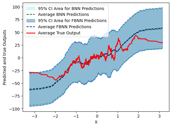
Figure 1: Comparison of 95% CI and mean prediction based on simulated data.

4.1.2 Wine Quality Data

As the first real dataset for the regression case, we use the Wine Quality data, provided by [51]. This dataset contains various physicochemical properties of different wines, and the target variable is the quality rating.

Initially, we trained a DNN model with a total of $J=241$ model parameters. Subsequently, we evaluated this model on a test dataset, recording both the model accuracy on the test dataset and the total training time.

For BNN models, we first place a prior distribution, $\boldsymbol{\mathcal{N}(0,1I)}$, on the potential model parameters, denoted as p($\theta$). The BNN models also featured $J=241$ total model parameters.

Based on the results shown in Table 1, DNN privides the best MSE at 0.43. However, as stated before, it lacks the capability to quantify uncertainty. Both BNN-SGHMC and FBNN(SGHMC-pCN) provide similar MSE values of 0.53 and 0.52 respectively. While BNN-SGHMC has slightly better CP, FBNN(SGHMC-pCN) is more computationally efficient. Figure 2 shows the prediction mean and CI for both methods.

Figure 2: Comparison of 95% CI and mean prediction based on the Wine Quality data.

4.1.3 Boston Housing Data

The Boston housing data was collected in 1978. Each of the 506 entries represent aggregated data of 14 features for homes from various suburbs in Boston. For this dataset, we followed CES steps similar to the Wine Quality dataset but with different number of model parameters ($J$=3009); the emulator has 3 hidden layers, but larger number of nodes (2048, 1024, 512).

For this example, the DNN achieves an MSE of 3.21. BNN-SGHMC and BNN-pCN exhibit comparable MSE values at 3.83 and 3.25, respectively, with BNN-pCN showing slightly better CP (89.3%) than BNN-SGHMC (85.3%). Among the FBNN variants, FBNN(SGHMC-pCN) stands out with a notable balance between MSE (3.82), CP (71.1%), and computational efficiency, completing the task in just 91 seconds. This model significantly outperforms BNN-SGHMC in terms of both speed-up (11.94) and CP, showcasing its effectiveness in uncertainty quantification. Figure 3 shows the 95% CIs and mean predictions of both BNN-SGHMC and FBNN(SGHMC-pCN).

Figure 3: Comparison of 95% CI and mean prediction based on the Boston Housing data.

Dataset	Method	Acc	Time(s)	ESS(min,med,max)	minESS/s	spdup
Simulated Dataset	DNN	96%	18
	BNN-SGHMC	96%	889	(23.0, 189.5, 1468.6)	0.03	1
	BNN-pCN	96%	1015	(38.5, 176.5, 1351.6)	0.04	1.46
	FBNN(pCN-SGHMC)	92%	105	(132.9, 947.1, 1539.1)	1.26	48.92
	FBNN(pCN-pCN)	90%	105	(147.9, 861.6, 1535.1)	1.41	54.44
	FBNN(SGHMC-SGHMC)	95%	97	(153.2, 871.7, 1520.8)	1.57	61.04
	FBNN(SGHMC-pCN)	96%	92	(153.1, 871.7, 1520.7)	1.67	64.32
Adult Dataset	DNN	85%	426
	BNN-SGHMC	83%	5979	(16.0, 202.9, 1520.0)	0.002	1
	BNN-pCN	83%	6227	(8.8, 117.3, 1518.4)	0.001	0.52
	FBNN(pCN-SGHMC)	82%	642	(87.5, 892.2, 1539.7)	0.13	50.93
	FBNN(pCN-pCN)	82%	639	(88.1, 890.4, 1540.0)	0.12	51.52
	FBNN(SGHMC-SGHMC)	83%	612	(68.6, 941.7, 1541.8)	0.12	41.88
	FBNN(SGHMC-pCN)	84%	609	(89.5, 875.9, 1539.9)	0.15	54.91

Table 2: Performance of various deep learning methods based on classification problems.

Classification

We also evaluate our method based on a set of simulated and real classification problems. The results are provided in Table 2.

4.2.1 Simulated Data

In this section we focus on a binary classification problem using simulate data. The data setup involves a similar structure to the regression case, with the key difference being in the response variable, loss functions, and the architecture of the DNN emulator. Here, the emulator has two layers with ReLU activation functions for the hidden layers and sigmoid activation for the output layer. All methods have similar performance in terms of accuracy. As before, FBNN(SGHMC-pCN) stands out with the highest Effective Sample Size (ESS) per second at 1.67; it achieves the highest speed up, 64.32, demonstrating its computational efficiency in comparison to BNN-SGHMC.

4.2.2 Adult Data

Next, we use the Adult dataset, discussed in [52]. This dataset comprises a relatively larger sample size of 40,434 data points, each described by 14 distinct features. All BNN and FBNN versions contain a complex structure with 2,761 internal model parameters. The classification task for the Adult dataset involves predicting whether an individual will earn more or less than $50,000 per year.

All methods provide similar accuracy rates, with FBNN(SGHMC-pCN) emerging again as the most computationally efficient method for uncertainty quantification, with the speed-up value of 54.91 compared to the baseline BNN approach.

Conclusion

In this paper, we have proposed an innovative CES framework called FBNN, specifically designed to enhance the computational efficiency and scalability of BNN for high-dimensional data. Our primary goal is to provide a robust solution for uncertainty quantification in high-dimensional spaces, leveraging the power of Bayesian principles while mitigating the computational bottlenecks traditionally associated with BNN.

In our numerical experiments, we have successfully applied various variants of FBNN, including different configurations with BNN, to regression and classification tasks on both synthetic and real datasets. Remarkably, the FBNN variant incorporating SGHMC for calibration and pCN for sampling, denoted as FBNN(SGHMC-pCN), not only matches the predictive accuracy of traditional BNN but also offers substantial computational advantages. The superior performance of the FBNN variant employing SGHMC for calibration and pCN for sampling can be attributed to the complementary strengths of these two samplers. SGHMC excels at broad exploration of the parameter space, providing an effective means for understanding the global structure during the calibration step. On the other hand, pCN is adept at efficient sampling around modes, offering a valuable tool for capturing local intricacies in the distribution during the final sampling step. By combining these samplers in the FBNN model, we achieve a balanced approach between exploration (calibration with SGHMC) and exploitation (final sampling with pCN).

Future work could involve extending our method to more complex problems (e.g., spatiotemporal data) and complex network structures (e.g., graph neural networks). Additionally, future research could focus on improving the emulation step by optimizing the DNN architecture. Finally, our method could be further improved by embedding the sampling algorithm in an adaptive framework similar to the method of [17].

References

- [1] J. Cheng, P.-s. Wang, G. Li, Q.-h. Hu, and H.-q. Lu, “Recent advances in efficient computation of deep convolutional neural networks,” Frontiers of Information Technology & Electronic Engineering, vol. 19, pp. 64–77, 2018.
- [2] Y. LeCun, L. Bottou, Y. Bengio, and P. Haffner, “Gradient-based learning applied to document recognition,” Proceedings of the IEEE, vol. 86, no. 11, pp. 2278–2324, 1998.
- [3] V. Sze, Y.-H. Chen, T.-J. Yang, and J. S. Emer, “Efficient processing of deep neural networks: A tutorial and survey,” Proceedings of the IEEE, vol. 105, no. 12, pp. 2295–2329, 2017.
- [4] J. Su, D. V. Vargas, and K. Sakurai, “One pixel attack for fooling deep neural networks,” IEEE Transactions on Evolutionary Computation, vol. 23, no. 5, pp. 828–841, 2019.
- [5] Y. Kwon, J.-H. Won, B. J. Kim, and M. C. Paik, “Uncertainty quantification using bayesian neural networks in classification: Application to ischemic stroke lesion segmentation,” in Medical Imaging with Deep Learning, 2022.
- [6] D. J. MacKay, “A practical bayesian framework for backpropagation networks,” Neural computation, vol. 4, no. 3, pp. 448–472, 1992.
- [7] R. M. Neal, Bayesian learning for neural networks, vol. 118. Springer Science & Business Media, 2012.
- [8] L. V. Jospin, H. Laga, F. Boussaid, W. Buntine, and M. Bennamoun, “Hands-on bayesian neural networks—a tutorial for deep learning users,” IEEE Computational Intelligence Magazine, vol. 17, no. 2, pp. 29–48, 2022.
- [9] M. Welling and Y. W. Teh, “Bayesian learning via stochastic gradient langevin dynamics,” in Proceedings of the 28th International Conference on Machine Learning (ICML-11), pp. 681–688, 2011.
- [10] B. Shahbaba, S. Lan, W. Johnson, and R. Neal, “Split Hamiltonian Monte Carlo,” Statistics and Computing, vol. 24, no. 3, pp. 339–349, 2014.
- [11] S. Ahn, B. Shahbaba, and M. Welling, “Distributed Stochastic Gradient MCMC,” in International Conference on Machine Learning, 2014.
- [12] M. Hoffman and A. Gelman, “The No-U-Turn Sampler: Adaptively Setting Path Lengths in Hamiltonian Monte Carlo.” arxiv.org/abs/1111.4246, 2011.
- [13] A. Beskos, M. Girolami, S. Lan, P. E. Farrell, and A. M. Stuart, “Geometric mcmc for infinite-dimensional inverse problems,” Journal of Computational Physics, vol. 335, pp. 327–351, 2017.
- [14] T. Cui, K. J. Law, and Y. M. Marzouk, “Dimension-independent likelihood-informed mcmc,” Journal of Computational Physics, vol. 304, pp. 109–137, 2016.
- [15] C. Zhang, B. Shahbaba, and H. Zhao, “Precomputing strategy for Hamiltonian Monte Carlo method based on regularity in parameter space,” Computational Statistics, vol. 32, no. 1, 2017.
- [16] C. Zhang, B. Shahbaba, and H. Zhao, “Hamiltonian Monte Carlo acceleration using surrogate functions with random bases,” Statistics and Computing, vol. 27, no. 6, 2017.
- [17] C. Zhang, B. Shahbaba, and H. Zhao, “Variational hamiltonian Monte Carlo via score matching,” Bayesian Analysis, vol. 13, no. 2, 2018.
- [18] L. Li, A. Holbrook, B. Shahbaba, and P. Baldi, “Neural Network Gradient Hamiltonian Monte Carlo,” Computational Statistics, vol. 34, no. 1, pp. 281–299, 2019.
- [19] E. Cleary, A. Garbuno-Inigo, S. Lan, T. Schneider, and A. M. Stuart, “Calibrate, emulate, sample,” Journal of Computational Physics, vol. 424, p. 109716, jan 2021.
- [20] S. Lan, S. Li, and B. Shahbaba, “Scaling up bayesian uncertainty quantification for inverse problems using deep neural networks,” SIAM/ASA Journal on Uncertainty Quantification, vol. 10, no. 4, pp. 1684–1713, 2022.
- [21] C. Currin, T. Mitchell, M. Morris, and D. Ylvisaker, “A bayesian approach to the design and analysis of computer experiments,” tech. rep., Oak Ridge National Lab., TN (USA), 1988.
- [22] J. Oakley and A. O’Hagan, “Bayesian inference for the uncertainty distribution of computer model outputs,” Biometrika, vol. 89, pp. 769–784, 12 2002.
- [23] J. E. Oakley and A. O’Hagan, “Probabilistic sensitivity analysis of complex models: A bayesian approach,” Journal of the Royal Statistical Society. Series B (Statistical Methodology), vol. 66, no. 3, pp. 751–769, 2004.
- [24] M. C. Kennedy and A. O’Hagan, “Bayesian Calibration of Computer Models,” Journal of the Royal Statistical Society Series B: Statistical Methodology, vol. 63, pp. 425–464, 01 2002.
- [25] D. Higdon, M. Kennedy, J. C. Cavendish, J. A. Cafeo, and R. D. Ryne, “Combining field data and computer simulations for calibration and prediction,” SIAM Journal on Scientific Computing, vol. 26, no. 2, pp. 448–466, 2004.
- [26] A. O’Hagan, “Bayesian analysis of computer code outputs: A tutorial,” Reliability Engineering & System Safety, vol. 91, no. 10, pp. 1290–1300, 2006. The Fourth International Conference on Sensitivity Analysis of Model Output (SAMO 2004).
- [27] S. Lan, J. A. Palacios, M. Karcher, V. Minin, and B. Shahbaba, “An efficient bayesian inference framework for coalescent-based nonparametric phylodynamics,” Bioinformatics, vol. 31, no. 20, pp. 3282–3289, 2015.
- [28] H. Liu, Y.-S. Ong, X. Shen, and J. Cai, “When gaussian process meets big data: A review of scalable gps,” IEEE transactions on neural networks and learning systems, vol. 31, no. 11, pp. 4405–4423, 2020.
- [29] E. V. Bonilla, K. Chai, and C. Williams, “Multi-task gaussian process prediction,” Advances in neural information processing systems, vol. 20, 2007.
- [30] J. Gardner, G. Pleiss, K. Q. Weinberger, D. Bindel, and A. G. Wilson, “Gpytorch: Blackbox matrix-matrix gaussian process inference with gpu acceleration,” Advances in neural information processing systems, vol. 31, 2018.
- [31] M. W. Seeger, C. K. Williams, and N. D. Lawrence, “Fast forward selection to speed up sparse gaussian process regression,” in International Workshop on Artificial Intelligence and Statistics, pp. 254–261, PMLR, 2003.
- [32] S. Lan, S. Li, and B. Shahbaba, “Scaling up bayesian uncertainty quantification for inverse problems using deep neural networks,” 2022.
- [33] S. Dargan, M. Kumar, M. R. Ayyagari, and G. Kumar, “A survey of deep learning and its applications: a new paradigm to machine learning,” Archives of Computational Methods in Engineering, vol. 27, pp. 1071–1092, 2020.
- [34] A. Gelman, W. R. Gilks, and G. O. Roberts, “Weak convergence and optimal scaling of random walk metropolis algorithms,” The annals of applied probability, vol. 7, no. 1, pp. 110–120, 1997.
- [35] G. O. Roberts and J. S. Rosenthal, “Optimal scaling of discrete approximations to langevin diffusions,” Journal of the Royal Statistical Society: Series B (Statistical Methodology), vol. 60, no. 1, pp. 255–268, 1998.
- [36] A. Beskos, G. Roberts, and A. Stuart, “Optimal scalings for local Metropolis–Hastings chains on nonproduct targets in high dimensions,” The Annals of Applied Probability, vol. 19, no. 3, pp. 863 – 898, 2009.
- [37] A. Beskos, “A stable manifold mcmc method for high dimensions,” Statistics & Probability Letters, vol. 90, pp. 46–52, 2014.
- [38] A. Beskos, F. J. Pinski, J. M. Sanz-Serna, and A. M. Stuart, “Hybrid monte carlo on hilbert spaces,” Stochastic Processes and their Applications, vol. 121, no. 10, pp. 2201–2230, 2011.
- [39] S. L. Cotter, G. O. Roberts, A. M. Stuart, and D. White, “MCMC Methods for Functions: Modifying Old Algorithms to Make Them Faster,” Statistical Science, vol. 28, no. 3, pp. 424 – 446, 2013.
- [40] K. J. Law, “Proposals which speed up function-space mcmc,” Journal of Computational and Applied Mathematics, vol. 262, pp. 127–138, 2014.
- [41] C. Andrieu, N. De Freitas, A. Doucet, and M. I. Jordan, “An introduction to mcmc for machine learning,” Machine learning, vol. 50, pp. 5–43, 2003.
- [42] S. Chib and E. Greenberg, “Understanding the metropolis-hastings algorithm,” The american statistician, vol. 49, no. 4, pp. 327–335, 1995.
- [43] C. P. Robert, G. Casella, and G. Casella, Monte Carlo statistical methods, vol. 2. Springer, 1999.
- [44] R. M. Neal et al., “Mcmc using hamiltonian dynamics,” Handbook of markov chain monte carlo, vol. 2, no. 11, p. 2, 2011.
- [45] T. Chen, E. Fox, and C. Guestrin, “Stochastic gradient hamiltonian monte carlo,” in International conference on machine learning, pp. 1683–1691, PMLR, 2014.
- [46] S. C.-H. Yang, W. K. Vong, R. B. Sojitra, T. Folke, and P. Shafto, “Mitigating belief projection in explainable artificial intelligence via bayesian teaching,” Scientific reports, vol. 11, no. 1, p. 9863, 2021.
- [47] C. Guo, G. Pleiss, Y. Sun, and K. Q. Weinberger, “On calibration of modern neural networks,” in Proceedings of the 34th International Conference on Machine Learning (D. Precup and Y. W. Teh, eds.), vol. 70 of Proceedings of Machine Learning Research, pp. 1321–1330, PMLR, 06–11 Aug 2017.
- [48] J. Nixon, M. W. Dusenberry, L. Zhang, G. Jerfel, and D. Tran, “Measuring calibration in deep learning,” in Proceedings of the IEEE/CVF Conference on Computer Vision and Pattern Recognition (CVPR) Workshops, June 2019.
- [49] G. Da Prato and J. Zabczyk, Stochastic equations in infinite dimensions. Cambridge university press, 2014.
- [50] M. Hairer, A. M. Stuart, and J. Voss, “Sampling conditioned diffusions,” Trends in stochastic analysis, vol. 353, pp. 159–186, 2009.
- [51] P. Cortez, A. Cerdeira, F. Almeida, T. Matos, and J. Reis, “Wine Quality.” UCI Machine Learning Repository, 2009. DOI: https://doi.org/10.24432/C56S3T.
- [52] B. Becker and R. Kohavi, “Adult.” UCI Machine Learning Repository, 1996.